Embed Size (px)
Citation preview
UNIVERSITA DEL SALENTOFACOLTA DI SCIENZE MM. FF. NN.
Dott.ssa Maria Rita COLUCCIA
PhD Thesis
Electron Drift Velocityand Amplification
in Resistive Plate Counters (RPC)
operating withthe ATLAS Gas Mixture
Supervisors:Prof. Edoardo GORINI
Dott.ssa Margherita PRIMAVERA
Dottorato di Ricerca in Fisica XIX CicloSettore Scientifico FIS/04
Index
Introduction 1
1 The Large Hadron Collider at CERN 31.1 The Large Hadron Collider . . . . . . . . . . . . . . . . . . . . 3
1.1.1 Lattice layout . . . . . . . . . . . . . . . . . . . . . . . 51.1.2 Accelerator Magnets . . . . . . . . . . . . . . . . . . . 81.1.3 Radio-frequency Acceleration System . . . . . . . . . . 8
1.2 The LHC Physics Program . . . . . . . . . . . . . . . . . . . . 91.2.1 Higgs Search . . . . . . . . . . . . . . . . . . . . . . . 91.2.2 New Physics Search . . . . . . . . . . . . . . . . . . . . 15
2 Experiments at LHC and the ATLAS Muon Spectrometer 182.1 Experimental challenges at LHC . . . . . . . . . . . . . . . . . 182.2 General Purpose Experiments at LHC . . . . . . . . . . . . . 19
2.2.1 A Toroidal LHC Apparatus (ATLAS) . . . . . . . . . . 202.2.2 The Compact Muon Solenoid (CMS) . . . . . . . . . . 21
2.3 The ATLAS Muon Spectrometer . . . . . . . . . . . . . . . . 232.3.1 The Muon Spectrometer Design . . . . . . . . . . . . . 232.3.2 Tracking Chambers . . . . . . . . . . . . . . . . . . . . 272.3.3 Trigger chambers . . . . . . . . . . . . . . . . . . . . . 29
3 Resistive Plate Counters 333.1 Introduction . . . . . . . . . . . . . . . . . . . . . . . . . . . . 333.2 Resistive Plate Chambers . . . . . . . . . . . . . . . . . . . . 343.3 Particle Energy Loss in the Matter . . . . . . . . . . . . . . . 353.4 Fundamental Processes in Gas Detectors . . . . . . . . . . . . 37
3.4.1 Electrons Diffusion . . . . . . . . . . . . . . . . . . . . 383.4.2 Electron Drift . . . . . . . . . . . . . . . . . . . . . . . 39
Index 3
3.4.3 Electron Recombination and Capture . . . . . . . . . . 403.4.4 Electron Multiplication . . . . . . . . . . . . . . . . . . 41
3.5 Signal Readout in RPC . . . . . . . . . . . . . . . . . . . . . . 443.5.1 Ramo’s theorem: the ‘k factor’ . . . . . . . . . . . . . 443.5.2 Signal Induced by an Electron Avalanche . . . . . . . . 463.5.3 Single Electron Avalanche Fluctuation . . . . . . . . . 47
4 Experimental Set-up and Measurement Technique 494.1 Introduction . . . . . . . . . . . . . . . . . . . . . . . . . . . . 494.2 Gas Ionization by UV Laser . . . . . . . . . . . . . . . . . . . 494.3 Experimental Set-up . . . . . . . . . . . . . . . . . . . . . . . 53
4.3.1 RPC Prototypes . . . . . . . . . . . . . . . . . . . . . 544.3.2 Optical System and Laser Alignment . . . . . . . . . . 554.3.3 Gas System . . . . . . . . . . . . . . . . . . . . . . . . 574.3.4 High Voltage System . . . . . . . . . . . . . . . . . . . 614.3.5 Micro-metric Movements System . . . . . . . . . . . . 624.3.6 Nitrogen Laser . . . . . . . . . . . . . . . . . . . . . . 624.3.7 Signal Acquisition . . . . . . . . . . . . . . . . . . . . . 66
4.4 Acquisition and Control System . . . . . . . . . . . . . . . . . 684.4.1 The Graphical User Interface GUI . . . . . . . . . . . . 694.4.2 The MySQL Database . . . . . . . . . . . . . . . . . . 724.4.3 The DAQ-DCS Loop . . . . . . . . . . . . . . . . . . . 734.4.4 The Off-line Software Analysis . . . . . . . . . . . . . . 74
5 Experimental Results 755.1 Introduction . . . . . . . . . . . . . . . . . . . . . . . . . . . . 755.2 Electron Avalanche Signal . . . . . . . . . . . . . . . . . . . . 755.3 Laser Ionization Source Set-up . . . . . . . . . . . . . . . . . . 765.4 Electron Drift Velocity Measurements . . . . . . . . . . . . . . 83
5.4.1 Results and comparison with MAGBOLTZ . . . . . . . 845.5 RPC I prototype measurements: a good lesson . . . . . . . . . 895.6 Gas amplification Study . . . . . . . . . . . . . . . . . . . . . 92
5.6.1 Saturated Avalanche Regime . . . . . . . . . . . . . . . 925.6.2 Avalanche Charge Spectra . . . . . . . . . . . . . . . . 935.6.3 Single Avalanche Charge Spectra . . . . . . . . . . . . 945.6.4 Charge Spectra Characterization . . . . . . . . . . . . 955.6.5 Measurements of the effective Townsend coefficient . . 985.6.6 Avalanche Charge Spectra with no SF6 . . . . . . . . . 99
Index 4
5.7 Humidified Gas Mixture . . . . . . . . . . . . . . . . . . . . . 1015.8 Mass Spectrometry Measurements . . . . . . . . . . . . . . . . 103
Conclusions 107
A Special ATLAS RPC Chamber tests at CERN 109A.0.1 Leakage Current Tests . . . . . . . . . . . . . . . . . . 111A.0.2 Ground Stability Tests . . . . . . . . . . . . . . . . . . 112
Bibliography 116
Introduction
This work is mainly devoted to the measurements of electron transportand amplification properties of the gas mixture used for the Resistive PlateCounters (RPC’s) in the ATLAS experiment at the Large Hadron Collider(LHC) under construction at CERN in Geneva, where RPC are employed asmuon trigger detectors.
This gas mixture has three components: 94.7 % of Tetrafluoroethane(C2H2F4) as main component, 5 % isobutane (C4H10) as photons quencherand 0.3 % SF6, in order to inhibit streamers development and it allows tooperate the detector in the so called saturated avalanche mode, instead of themore conventional streamer mode, until now and presently widely adoptedby experiments. The reason for operating in this regime is to increase thedetector rate capability up to ∼1 kHz/cm2 (about one order of magnitudeof the usual values reached by RPC operating in streamer), to reduce agingphenomena and to maintain good efficiency and time resolution.
The knowledge of the underlying physical processes in the RPC detectorsallows for developing Montecarlo simulations of their behavior to becompared with experimental data. This is crucial in order to predict detectorperformances and to optimize detector designs. In literature, several authorsmade Montecarlo simulations of RPC’s operating in LHC [1, 2]. In theseworks the input fundamental gas parameters where extracted by the widelyused program MAGBOLTZ [3, 4], that allows to compute them for electronin various gases. In addition, these authors simulated avalanche fluctuationsin saturated avalanche regime with ad hoc assumption or by using specificmodels.
We measured directly the gas parameters and the avalanche fluctuationspectra in RPC ATLAS-like prototypes in Lecce INFN and PhysicsDepartments laboratory. A comparison of the measurement results withMAGBOLTZ calculation has been performed and a satisfying agreement
Introduction 2
has been found for both electron drift velocity and effective Townsend’scoefficient.
A N2 (λ = 337 nm) pulsed laser has been used to induce ionization inthe RPC prototype gas gap, since the use such source has the advantagesto generate primary electron (from a single up to hundred depending on thebeam intensity) localized in a small area around a lens focus. All the studiespresented here have been performed by using two small size RPC (10 × 20cm2) prototypes, RPC I and RPC II, having a 2 mm gas gap delimited by2mm-thick linseed-oil-treated Bakelite plates with a resistivity of about 1.4× 10¹¹ Ω cm and of about 1.71 × 10¹⁰ Ω cm respectively.
The measurement setup has been designed to take advantage of anexisting facility, but completely new dedicated Data Acquisition System(DAQ), Detector Control System (DCS) and on-line (offline analysis)software have been implemented.
This thesis is organized in 5 chapters.The first two chapters are dedicated to the description of the LHC physics
programs and to a brief overview of the ATLAS and CMS experiments,with more emphasis in the description of the ATLAS Muon Spectrometeryo which this work is in ultimate analysis finalized; a full description of theRPC detectors structure is presented in chapter 3, together with the physicsphenomena underlying their behavior.
Chapters 4 describes the laser ionization technique and its fruitfulemployment in calibrating gas detectors and the experimental setup in allits components, hardware and software.
Finally, Chapter 5 is dedicated to the discussion of the experimentalresults.
An appendix reports the quality assurance tests performed on the socalled special RPC detectors (S2 and S3) of the barrel trigger system andbefore their final installation in the ATLAS Muon Spectrometer. This workhas been entirely performed at CERN and represents a relevant part of theresearch activity during PHD period.
Chapter 1
The Large Hadron Collider atCERN
1.1 The Large Hadron Collider
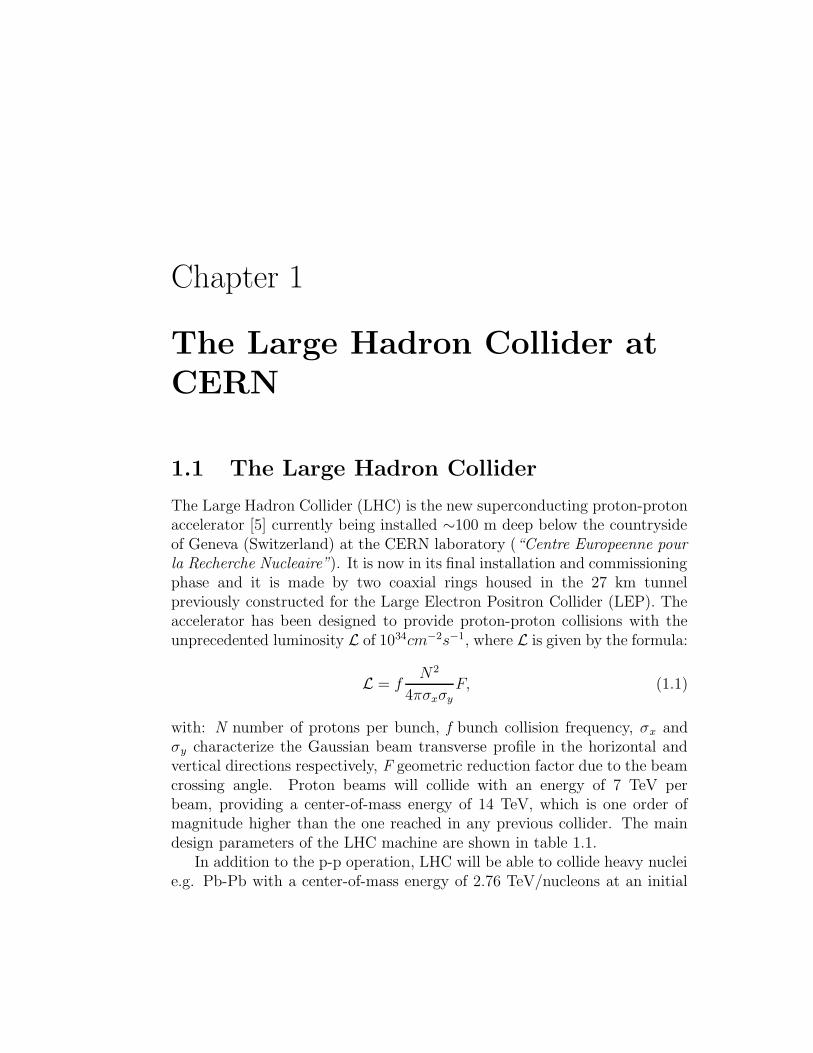
The Large Hadron Collider (LHC) is the new superconducting proton-protonaccelerator [5] currently being installed ∼100 m deep below the countrysideof Geneva (Switzerland) at the CERN laboratory (“Centre Europeenne pourla Recherche Nucleaire”). It is now in its final installation and commissioningphase and it is made by two coaxial rings housed in the 27 km tunnelpreviously constructed for the Large Electron Positron Collider (LEP). Theaccelerator has been designed to provide proton-proton collisions with theunprecedented luminosity L of 1034cm−2s−1, where L is given by the formula:
L = fN2
4πσxσy
F, (1.1)
with: N number of protons per bunch, f bunch collision frequency, σx andσy characterize the Gaussian beam transverse profile in the horizontal andvertical directions respectively, F geometric reduction factor due to the beamcrossing angle. Proton beams will collide with an energy of 7 TeV perbeam, providing a center-of-mass energy of 14 TeV, which is one order ofmagnitude higher than the one reached in any previous collider. The maindesign parameters of the LHC machine are shown in table 1.1.
In addition to the p-p operation, LHC will be able to collide heavy nucleie.g. Pb-Pb with a center-of-mass energy of 2.76 TeV/nucleons at an initial
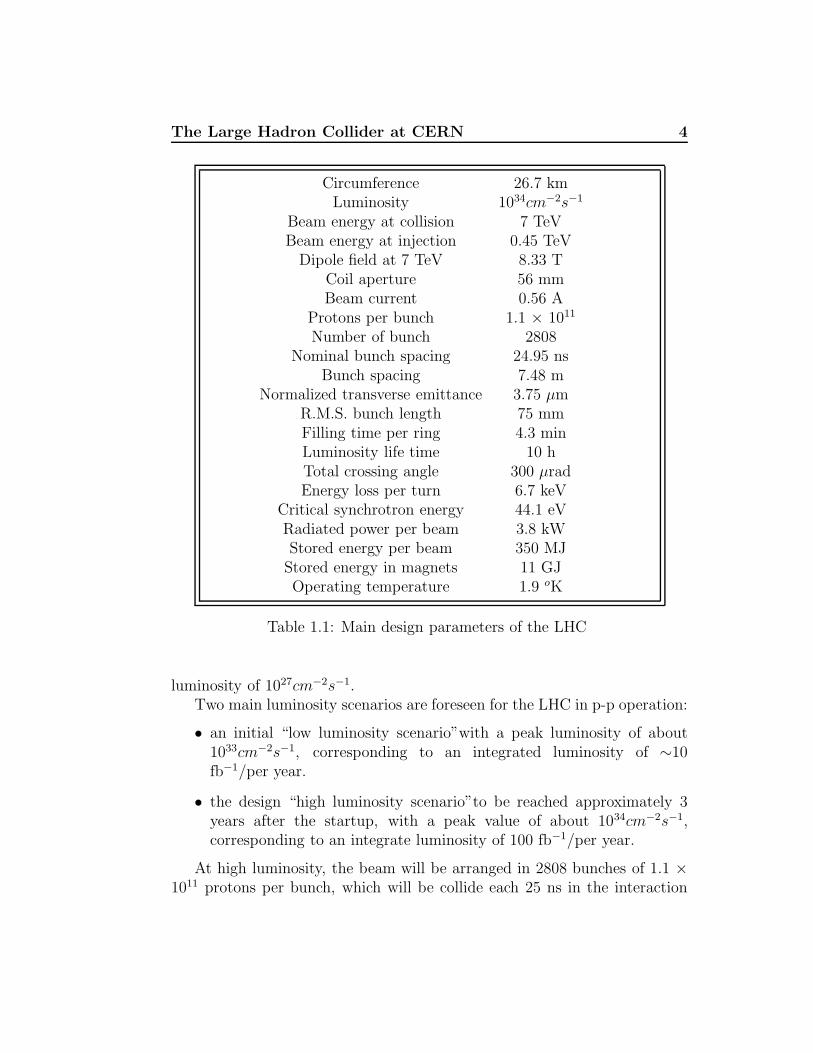
The Large Hadron Collider at CERN 4
Circumference 26.7 kmLuminosity 1034cm−2s−1
Beam energy at collision 7 TeVBeam energy at injection 0.45 TeV
Dipole field at 7 TeV 8.33 TCoil aperture 56 mmBeam current 0.56 A
Protons per bunch 1.1 × 10¹¹
Number of bunch 2808Nominal bunch spacing 24.95 ns
Bunch spacing 7.48 mNormalized transverse emittance 3.75 µm
R.M.S. bunch length 75 mmFilling time per ring 4.3 minLuminosity life time 10 hTotal crossing angle 300 µradEnergy loss per turn 6.7 keV
Critical synchrotron energy 44.1 eVRadiated power per beam 3.8 kWStored energy per beam 350 MJ
Stored energy in magnets 11 GJOperating temperature 1.9 oK
Table 1.1: Main design parameters of the LHC
luminosity of 1027cm−2s−1.Two main luminosity scenarios are foreseen for the LHC in p-p operation:
• an initial “low luminosity scenario”with a peak luminosity of about1033cm−2s−1, corresponding to an integrated luminosity of ∼10fb−1/per year.
• the design “high luminosity scenario”to be reached approximately 3years after the startup, with a peak value of about 1034cm−2s−1,corresponding to an integrate luminosity of 100 fb−1/per year.
At high luminosity, the beam will be arranged in 2808 bunches of 1.1 ×10¹¹ protons per bunch, which will be collide each 25 ns in the interaction
The Large Hadron Collider at CERN 5
regions (IR). Given a p-p inelastic cross section of about 100 mb at 14 TeV,about 23 p-p interactions per crossing and a total of about 700 chargedparticles with PT > 150 MeV will be produced.
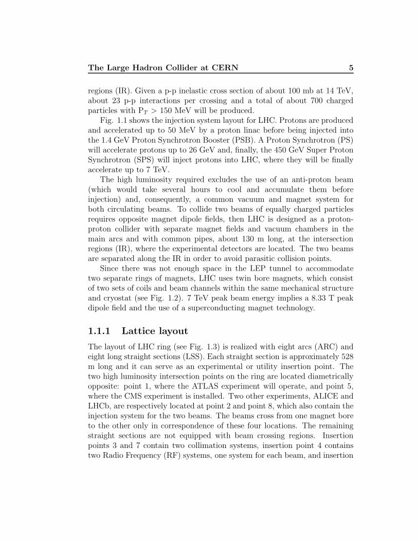
Fig. 1.1 shows the injection system layout for LHC. Protons are producedand accelerated up to 50 MeV by a proton linac before being injected intothe 1.4 GeV Proton Synchrotron Booster (PSB). A Proton Synchrotron (PS)will accelerate protons up to 26 GeV and, finally, the 450 GeV Super ProtonSynchrotron (SPS) will inject protons into LHC, where they will be finallyaccelerate up to 7 TeV.
The high luminosity required excludes the use of an anti-proton beam(which would take several hours to cool and accumulate them beforeinjection) and, consequently, a common vacuum and magnet system forboth circulating beams. To collide two beams of equally charged particlesrequires opposite magnet dipole fields, then LHC is designed as a proton-proton collider with separate magnet fields and vacuum chambers in themain arcs and with common pipes, about 130 m long, at the intersectionregions (IR), where the experimental detectors are located. The two beamsare separated along the IR in order to avoid parasitic collision points.
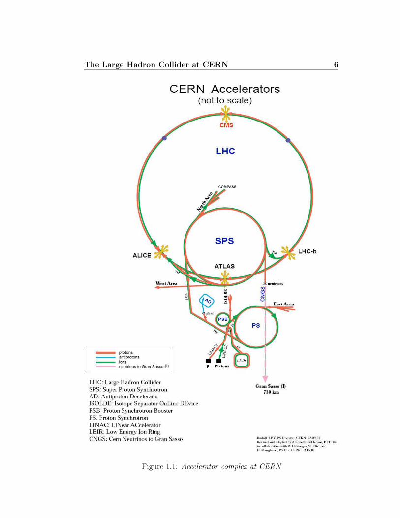
Since there was not enough space in the LEP tunnel to accommodatetwo separate rings of magnets, LHC uses twin bore magnets, which consistof two sets of coils and beam channels within the same mechanical structureand cryostat (see Fig. 1.2). 7 TeV peak beam energy implies a 8.33 T peakdipole field and the use of a superconducting magnet technology.
1.1.1 Lattice layout
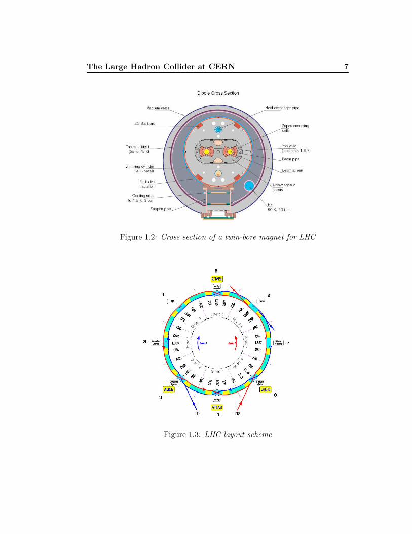
The layout of LHC ring (see Fig. 1.3) is realized with eight arcs (ARC) andeight long straight sections (LSS). Each straight section is approximately 528m long and it can serve as an experimental or utility insertion point. Thetwo high luminosity intersection points on the ring are located diametricallyopposite: point 1, where the ATLAS experiment will operate, and point 5,where the CMS experiment is installed. Two other experiments, ALICE andLHCb, are respectively located at point 2 and point 8, which also contain theinjection system for the two beams. The beams cross from one magnet boreto the other only in correspondence of these four locations. The remainingstraight sections are not equipped with beam crossing regions. Insertionpoints 3 and 7 contain two collimation systems, insertion point 4 containstwo Radio Frequency (RF) systems, one system for each beam, and insertion
The Large Hadron Collider at CERN 6
Figure 1.1: Accelerator complex at CERN
The Large Hadron Collider at CERN 7
Figure 1.2: Cross section of a twin-bore magnet for LHC
Figure 1.3: LHC layout scheme
The Large Hadron Collider at CERN 8
point 6 contains the beam dumps, ensuring an independent abort system forthe two beams.
In order to focus the beams in both horizontal and vertical planes, asuccession of focusing and defocusing quadrupole magnets is required: FODOstructures. The LHC lattice is composed of 23 regular FODO cells per arc.Each cell is 106,9 m long and is made of six dipoles 15 m long and two shortstraight sections 6.6 m long containing the main quadrupoles and multipolescorrectors.
1.1.2 Accelerator Magnets
LHC contains more than 7000 superconducting magnets. The mosttechnologically challenging are the 1232 superconducting dipoles and the 392quadrupoles in the arcs.
The challenge for the LHC dipole magnets is to have the highestbending strength making use of the well-proven technology based on Nb-Tisuperconducting cable. To increase the performance of Nb-Ti, the cooling ofthe superconductors to a temperature below 2 oK, using super-fluid helium,is required. In such a way, an extra 20% gain is attainable in the centralfield value, with respect to nowadays operating superconductor accelerators,cooled with super-fluid helium at a temperature slightly above 4.2 oK. Onthe other hand, at such a low temperature, the superconducting cable heatcapacity decreases almost an order of magnitude, making easier to trigger aquench.
1.1.3 Radio-frequency Acceleration System
The Radio-Frequency (RF) system provides the longitudinal electric field forproton acceleration and is located at insertion point 4.
It is made of single-cell superconducting cavities with large beam tubevery similar to those designed for the high current e+e− factories. There aretwo RF systems (one for each beam), each one composed by eight 400 MHzcavities, which are grouped by four in the two cryogenic modules.
The Large Hadron Collider at CERN 9
1.2 The LHC Physics Program
LHC can be thought as a parton-parton collider with a large spread incollision energy. The effective luminosity of the proton collisions falls offrapidly with the center of mass energy. With an expected proton beamenergy of 7 TeV, LHC will study physics at the 1 TeV scale in the parton-parton system, extending the accessible energy range approximately by afactor of ten with respect to the one reached by previous collider.
The fundamental goal is to explore the physics processes underlyingthe electroweak symmetry breaking. This new high energy regime alsooffers a unique opportunity to search for New Physics. In addition, thehigh luminosity and cross sections make the LHC a unique factory for theproduction of heavy particles like the top quark.
The search for the Higgs boson [6], responsible of the mass generationmechanism in the Standard Model (SM), has motivated much of the designof the two general purpose experiments at LHC. Our knowledge about theSM Higgs boson can be summarized as follows:
• its mass is not specified by the theory, which provides only an upperbound of ∼ 1 TeV;
• direct searches performed at LEP have set a lower limit of mH > 114.4GeV [7];
• a global fit of the SM parameters to the data collected by variousmachines (LEP, Tevatron, SLC) gives a 95% C.L. upper bound on mH
of about 250 GeV [8];
• the current experimental knowledge favor a light Higgs boson.
1.2.1 Higgs Search
SM Higgs
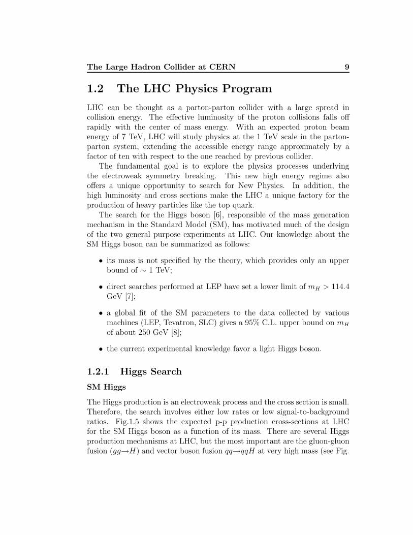
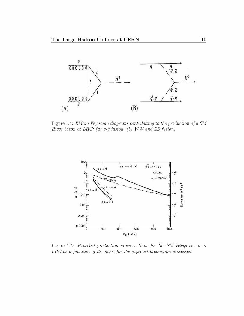
The Higgs production is an electroweak process and the cross section is small.Therefore, the search involves either low rates or low signal-to-backgroundratios. Fig.1.5 shows the expected p-p production cross-sections at LHCfor the SM Higgs boson as a function of its mass. There are several Higgsproduction mechanisms at LHC, but the most important are the gluon-gluonfusion (gg→H) and vector boson fusion qq→qqH at very high mass (see Fig.
The Large Hadron Collider at CERN 10
Figure 1.4: EMain Feynman diagrams contributing to the production of a SMHiggs boson at LHC: (a) g-g fusion, (b) WW and ZZ fusion.
Figure 1.5: Expected production cross-sections for the SM Higgs boson atLHC as a function of its mass, for the expected production processes.
The Large Hadron Collider at CERN 11
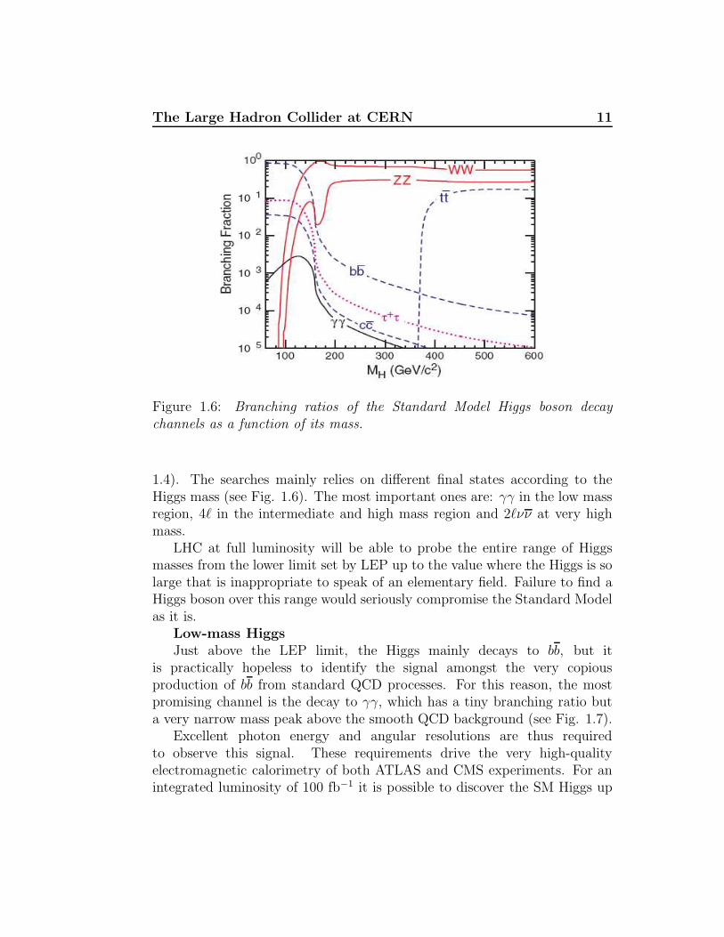
Figure 1.6: Branching ratios of the Standard Model Higgs boson decaychannels as a function of its mass.
1.4). The searches mainly relies on different final states according to theHiggs mass (see Fig. 1.6). The most important ones are: γγ in the low massregion, 4` in the intermediate and high mass region and 2`νν at very highmass.
LHC at full luminosity will be able to probe the entire range of Higgsmasses from the lower limit set by LEP up to the value where the Higgs is solarge that is inappropriate to speak of an elementary field. Failure to find aHiggs boson over this range would seriously compromise the Standard Modelas it is.
Low-mass HiggsJust above the LEP limit, the Higgs mainly decays to bb, but it
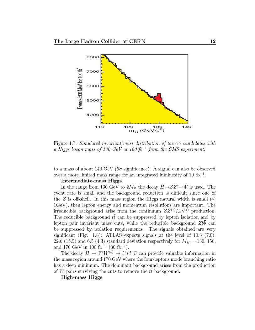
is practically hopeless to identify the signal amongst the very copiousproduction of bb from standard QCD processes. For this reason, the mostpromising channel is the decay to γγ, which has a tiny branching ratio buta very narrow mass peak above the smooth QCD background (see Fig. 1.7).
Excellent photon energy and angular resolutions are thus requiredto observe this signal. These requirements drive the very high-qualityelectromagnetic calorimetry of both ATLAS and CMS experiments. For anintegrated luminosity of 100 fb−1 it is possible to discover the SM Higgs up
The Large Hadron Collider at CERN 12
Figure 1.7: Simulated invariant mass distribution of the γγ candidates witha Higgs boson mass of 130 GeV at 100 fb−1 from the CMS experiment.
to a mass of about 140 GeV (5σ significance). A signal can also be observedover a more limited mass range for an integrated luminosity of 10 fb−1.
Intermediate-mass HiggsIn the range from 130 GeV to 2MZ the decay H→ZZ∗→4l is used. The
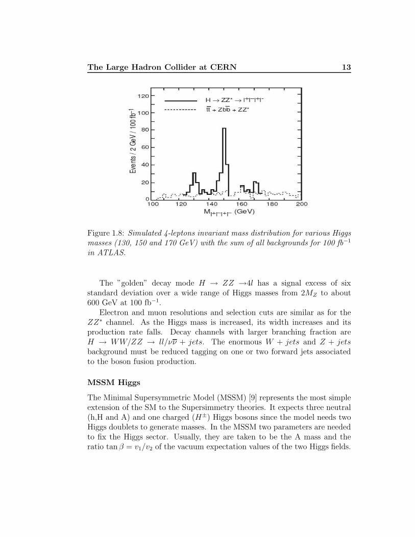
event rate is small and the background reduction is difficult since one ofthe Z is off-shell. In this mass region the Higgs natural width is small (≤1GeV), then lepton energy and momentum resolutions are important. Theirreducible background arise from the continuum ZZ (∗)/Zγ(∗) production.The reducible background tt can be suppressed by lepton isolation and bylepton pair invariant mass cuts, while the reducible background Zbb canbe suppressed by isolation requirements. The signals obtained are verysignificant (Fig. 1.8): ATLAS expects signals at the level of 10.3 (7.0),22.6 (15.5) and 6.5 (4.3) standard deviation respectively for MH = 130, 150,and 170 GeV in 100 fb−1 (30 fb−1).
The decay H → WW (∗) → l+νl−ν can provide valuable information inthe mass region around 170 GeV where the four-leptons mode branching ratiohas a deep minimum. The dominant background arises from the productionof W pairs surviving the cuts to remove the tt background.
High-mass Higgs
The Large Hadron Collider at CERN 13
Figure 1.8: Simulated 4-leptons invariant mass distribution for various Higgsmasses (130, 150 and 170 GeV) with the sum of all backgrounds for 100 fb−1
in ATLAS.
The ”golden” decay mode H → ZZ →4l has a signal excess of sixstandard deviation over a wide range of Higgs masses from 2MZ to about600 GeV at 100 fb−1.
Electron and muon resolutions and selection cuts are similar as for theZZ∗ channel. As the Higgs mass is increased, its width increases and itsproduction rate falls. Decay channels with larger branching fraction areH → WW/ZZ → ll/νν + jets. The enormous W + jets and Z + jetsbackground must be reduced tagging on one or two forward jets associatedto the boson fusion production.
MSSM Higgs
The Minimal Supersymmetric Model (MSSM) [9] represents the most simpleextension of the SM to the Supersimmetry theories. It expects three neutral(h,H and A) and one charged (H±) Higgs bosons since the model needs twoHiggs doublets to generate masses. In the MSSM two parameters are neededto fix the Higgs sector. Usually, they are taken to be the A mass and theratio tanβ = v1/v2 of the vacuum expectation values of the two Higgs fields.
The Large Hadron Collider at CERN 14
The phenomenological consequences of these parameters are:
• if tanβ is O(1), the coupling of the top quarks to Higgs bosons is muchlarger than that of the bottom quarks as is the case of the StandardModel;
• the charged Higgs boson H± is heavier than A (M 2H ∼ M2
A + M2W );
• H is heavier than A and, at large value of MA, the two bosons, A andH are almost degenerate;
• the mass of the lightest boson, h, increases with the mass of A andreaches a plateau for A heavier than about 200 GeV;
• in the limit of large mass A, the couplings of h become like those of theSM Higgs (decoupling limit);
• the couplings of A and H to charge 1/3 quarks and leptons are enhancedat large tan β relatively to those of a SM Higgs boson of the same mass;
• A does not couple to gauge boson pairs at lowest order and the couplingof H to them is suppressed at large tan β and large MA.
The decay modes used above in the case of the Standard Model Higgsboson can also be exploited in the SUSY Higgs case. h can be searched inthe final state γγ, as the branching ratio approaches that for the StandardModel Higgs for large MA values, and in h → bb. The decay A → γγ canalso be exploited. This has the advantage that, because A → ZZ, WW donot occur, the branching ratio is large enough for the signal to be usable forvalues of MA less than 2mt [10].
The decay H → ZZ∗ can be exploited but, at large values of MH , thedecay H → ZZ, which provides a very clear signal for the Standard ModelHiggs, is useless owing to its very small branching ratio.
In addition to these decay channels, several other possibilities are open updue to the larger number of Higgs bosons and possibly enhanced branchingratios. The most important are the decays of H/A to τ+τ− (stronglyenhanced if tan β is large) and H/A to µ+µ− (suppressed by a factor(mµ/mτ )
2 but with better resolution than H/A to τ+τ−), H → hh, A → Zhand A → tt.
The Large Hadron Collider at CERN 15
Search for Charged Higgs
It is possible to search for Charged Higgs. The decay t → bH± may competewith the standard t → bW± if it kinetically allowed. The H± decays to τνor cs depend on the value of the tan β. Over most of the range 1 <tanβ<50,the decay mode H± → τν dominates. The signal for H± production is thusan excess of tau’s produced in the tt events.
1.2.2 New Physics Search
Strong EWSB Dynamics
The precision electroweak measurements are consistent with a light Higgsboson but ElectroWeak Symmetry Breaking (EWSB) by new strongdynamics at the TeV scale cannot be excluded.
The couplings of longitudinally polarized gauge bosons at low energywill violate WW scattering amplitude unitarity around 1.5 TeV at whichpoint new physics must enter. In the Standard Model and its minimalsupersymmetric version, this is the perturbative coupling of the Higgs bosons.If no Higgs-like particle exists, then 1 TeV non-perturbative dynamics mustenter in the vector boson scattering amplitudes or new meson-like resonances(Technicolor).
In case of strongly interacting WW, WZ and ZZ, the signal appears asan excess of events over the Standard Model prediction of gauge boson pairsat large invariant mass. The favorite channel is qq → W±W±, which doesn’thave standard model background and the charge misidentification probabilityis negligible.
In case of Technicolor [11], theories predict Techni-resonances decay intovector boson pairs (or its longitudinal components) and quark pairs. Thesesignals are striking since they are produced with large cross sections. Thereare several signals to look for resonance mass peaks, such as Techni-rho(%T → WZ → 3lν, %T8 → jet − jet and %T → W (`ν)πT (bb)) and Techni-mesons (ηT → tt).
Supersymmetry (SUSY)
If SUSY is relevant to electroweak symmetry breaking, gluino and squarksmasses are less than O(1 TeV), although squarks might be heavier [12]. As
The Large Hadron Collider at CERN 16
many supersymmetric particles can be produced simultaneously at the LHCa model must be picked-up to simulate the events:
• SUGRA model [13] assumes that gravity is responsible for themediation of supersymmetry breaking and provides a natural candidatefor cold dark matter;
• GMSB model [14] assumes that the gauge interactions are responsiblefor the mediation of supersymmetry breaking and explains why flavourchanging neutral current effects are small;
• AMSB model assumes that anomaly mediation of supersymmetrybreaking, which is always present [15], is dominant.
Gluinos and squarks usually dominate the LHC SUSY production crosssection, which is of the order of 10 pb. Since these are strongly produced,it should be easy to separate SUSY from Standard Model backgrounds. Inthe minimal SUGRA (mSUGRA) model decays produce transverse missing
energy /ET from the undetected neutralino χ01’s (Lightest Supersimmetric
Particle, LSP), multiple jets and several numbers of leptons from theintermediate gauginos. A typical distribution featuring these signatures isthe one of the “effective mass”:
Meff = /ET +
4∑
i=1
pT,i (1.2)
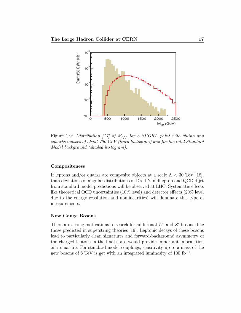
computed from the missing transverse energy and four the hardest jets in theevent (see Fig. 1.9).
GMSB models can give in the event additional photons or leptons or long-lived sleptons with high pT but β< 1, making the search easier. For R-parityviolating 1 model the decay χ0
1 → qqq(lll) gives signals at the LHC withvery large jet and leptons multiplicity. In all cases, SUSY can be discoveredat the LHC if the sparticle masses are in the expected range, and simplekinematic distributions can be used to estimate the approximate mass scale[16].
1R-parity is a multiplicative quantum number defined as R = (-1)2S+3B+L, where S isthe spin, B is the baryon number and L is the lepton number. All SM particles have R=1,while superpartners have R= -1. If R-parity is conserved, than a single SUSY particlecannot decay into just SM particles. In this case, LSP is absolutely stable. Anyway, itis possible that either baryon number or lepton number is violate, allowing the LSP todecay.
The Large Hadron Collider at CERN 17
Figure 1.9: Distribution [17] of Meff for a SUGRA point with gluino andsquarks masses of about 700 GeV (lined histogram) and for the total StandardModel background (shaded histogram).
Compositeness
If leptons and/or quarks are composite objects at a scale Λ < 30 TeV [18],than deviations of angular distributions of Drell-Yan dilepton and QCD dijetfrom standard model predictions will be observed at LHC. Systematic effectslike theoretical QCD uncertainties (10% level) and detector effects (20% leveldue to the energy resolution and nonlinearities) will dominate this type ofmeasurements.
New Gauge Bosons
There are strong motivations to search for additional W ′ and Z ′ bosons, likethose predicted in superstring theories [19]. Leptonic decays of these bosonslead to particularly clean signatures and forward-background asymmetry ofthe charged leptons in the final state would provide important informationon its nature. For standard model couplings, sensitivity up to a mass of thenew bosons of 6 TeV is get with an integrated luminosity of 100 fb−1.
Chapter 2
Experiments at LHC and theATLAS Muon Spectrometer
In the previous chapter the primary motivations to investigate physics atthe TeV scale with the Large Hadron Collider have been described. Twoout of four LHC detectors, ATLAS[16] and CMS[20], have been designedto exploit the full potential of the collider. Next sections are dedicated toa synthetic description of these two experiments, with the main focus onATLAS Muon Spectrometer, which is strictly related to the work describedin this thesis. The other two LHC experiments are: LHCb[21] a dedicated B-physics experiment designed to study CP violating and other rare phenomenain decays of hadrons with heavy flavours, in particular B mesons; ALICE[22]a dedicated heavy ions experiment designed to study the physics of stronglyinteracting matter and quark-gluon plasma in nucleus-nucleus collision.
2.1 Experimental challenges at LHC
The proton-proton inelastic cross-section at√
s = 14 TeV is roughly 100mb. At the design luminosity of 1034 cm−2s−1 general-purpose detectors willtherefore observe an event rate of 6.5 × 10⁸ inelastic events/s. This leads toa number of formidable experimental challenges[23].
The event selection process (“trigger”) must reduce the ∼ billioninteractions/s to no more than ∼ 102 events/s, for storage and subsequentanalysis. The short time between bunch crossings, 25 ns, has majorimplications for the design of the readout and trigger system. It is not feasible
Experiments at LHC and the ATLAS Muon Spectrometer 19
to make a trigger decision in this 25 ns, then new events may occur on everycrossing and, in order to avoid dead-time in the interval taken to make adecision, pipelined trigger processing and readout architectures are requiredwhere data from many bunch crossing are processed concurrently by a chainof processing elements. The first (“Level-1”) trigger decision takes about 3µs. During this time, more than 50% of which spent in signal transmission,the data must be stored in pipelines.
At the design luminosity a mean of 20 minimum-bias events will besuperimposed on the event of interest. This implies that around 1000charged particles will emerge from the interaction region every 25 ns. Theproduct of an interaction under study may be confused with those fromother interactions in the same bunch crossing. This problem, known aspileup, clearly becomes more severe when the response time of a detectorelement and its electronic signal is longer than 25 ns. The effect of pileupcan be reduced by using highly granular detectors with good time resolution,giving low occupancy at the expense of having large number of detectorchannels. The resulting millions of detector electronic channels require verygood synchronization.
The particles coming from the interaction region lead to high radiationlevels in the experimental area requiring radiation-hard detectors and front-end electronics.
Access for maintenance will be very difficult, time consuming and highlyrestricted. Hence, a long-term operational reliability is required.
The on-line trigger system has to analyze information that is continuouslygenerated at a rate of 40,000 Gbs−1 and reduce it to hundreds of Mbs−1 forstorage. The many petabytes of data that will be collected per year perexperiment have to be distributed for offline analysis to scientists locatedacross the globe. Data management problems deriving from this, havemotivated the application in this field of the Computing Grid techniques[24], with specific developments for LHC experiments [25].
2.2 General Purpose Experiments at LHC
ATLAS and CMS experiments are progressing in their construction to beready to take collision data in the spring 2008. Most of the experimentalchallenges come from the industries, that are trying to meet the schedulesfrom mass-production of components with the stringent quality requirements
Experiments at LHC and the ATLAS Muon Spectrometer 20
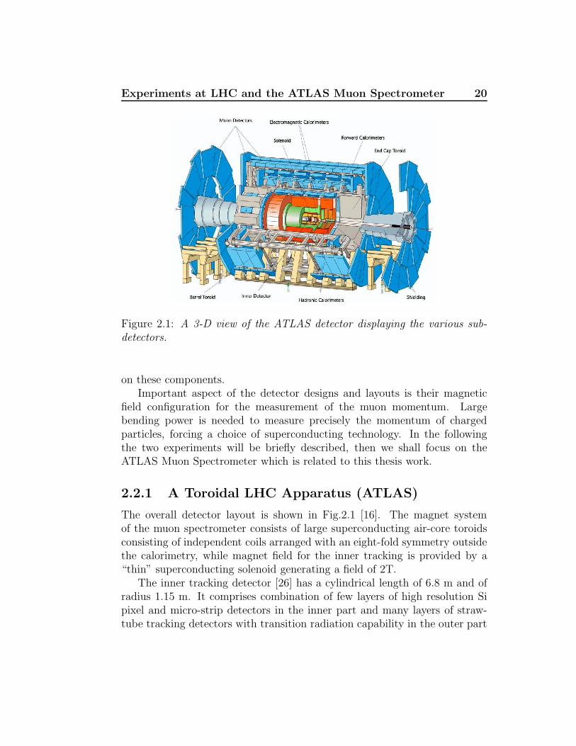
Figure 2.1: A 3-D view of the ATLAS detector displaying the various sub-detectors.
on these components.Important aspect of the detector designs and layouts is their magnetic
field configuration for the measurement of the muon momentum. Largebending power is needed to measure precisely the momentum of chargedparticles, forcing a choice of superconducting technology. In the followingthe two experiments will be briefly described, then we shall focus on theATLAS Muon Spectrometer which is related to this thesis work.
2.2.1 A Toroidal LHC Apparatus (ATLAS)
The overall detector layout is shown in Fig.2.1 [16]. The magnet systemof the muon spectrometer consists of large superconducting air-core toroidsconsisting of independent coils arranged with an eight-fold symmetry outsidethe calorimetry, while magnet field for the inner tracking is provided by a“thin” superconducting solenoid generating a field of 2T.
The inner tracking detector [26] has a cylindrical length of 6.8 m and ofradius 1.15 m. It comprises combination of few layers of high resolution Sipixel and micro-strip detectors in the inner part and many layers of straw-tube tracking detectors with transition radiation capability in the outer part
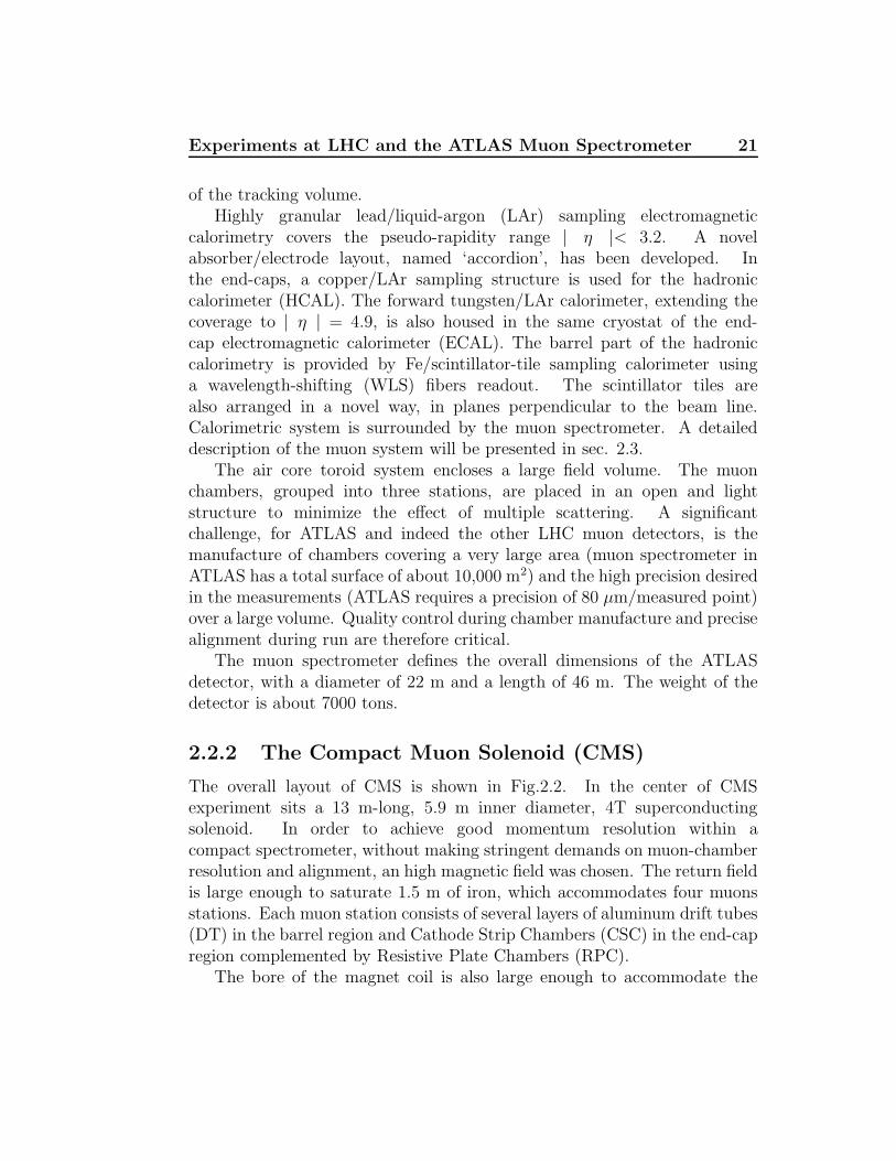
Experiments at LHC and the ATLAS Muon Spectrometer 21
of the tracking volume.Highly granular lead/liquid-argon (LAr) sampling electromagnetic
calorimetry covers the pseudo-rapidity range | η |< 3.2. A novelabsorber/electrode layout, named ‘accordion’, has been developed. Inthe end-caps, a copper/LAr sampling structure is used for the hadroniccalorimeter (HCAL). The forward tungsten/LAr calorimeter, extending thecoverage to | η | = 4.9, is also housed in the same cryostat of the end-cap electromagnetic calorimeter (ECAL). The barrel part of the hadroniccalorimetry is provided by Fe/scintillator-tile sampling calorimeter usinga wavelength-shifting (WLS) fibers readout. The scintillator tiles arealso arranged in a novel way, in planes perpendicular to the beam line.Calorimetric system is surrounded by the muon spectrometer. A detaileddescription of the muon system will be presented in sec. 2.3.
The air core toroid system encloses a large field volume. The muonchambers, grouped into three stations, are placed in an open and lightstructure to minimize the effect of multiple scattering. A significantchallenge, for ATLAS and indeed the other LHC muon detectors, is themanufacture of chambers covering a very large area (muon spectrometer inATLAS has a total surface of about 10,000 m2) and the high precision desiredin the measurements (ATLAS requires a precision of 80 µm/measured point)over a large volume. Quality control during chamber manufacture and precisealignment during run are therefore critical.
The muon spectrometer defines the overall dimensions of the ATLASdetector, with a diameter of 22 m and a length of 46 m. The weight of thedetector is about 7000 tons.
2.2.2 The Compact Muon Solenoid (CMS)
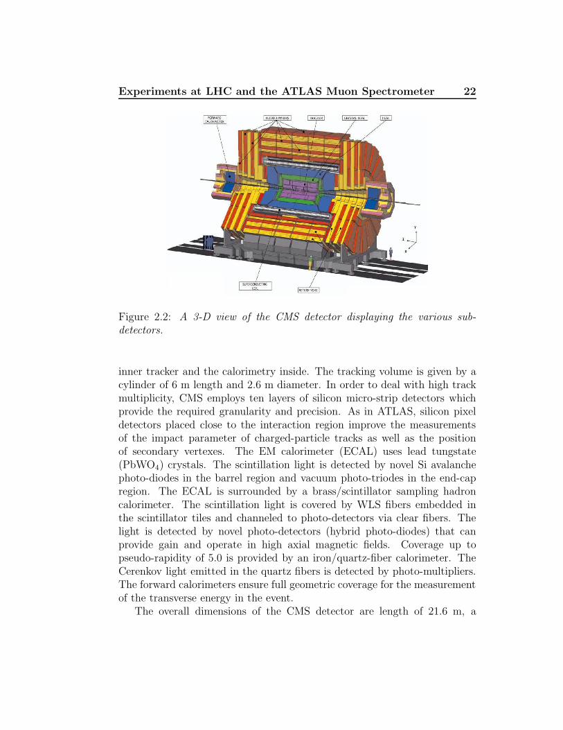
The overall layout of CMS is shown in Fig.2.2. In the center of CMSexperiment sits a 13 m-long, 5.9 m inner diameter, 4T superconductingsolenoid. In order to achieve good momentum resolution within acompact spectrometer, without making stringent demands on muon-chamberresolution and alignment, an high magnetic field was chosen. The return fieldis large enough to saturate 1.5 m of iron, which accommodates four muonsstations. Each muon station consists of several layers of aluminum drift tubes(DT) in the barrel region and Cathode Strip Chambers (CSC) in the end-capregion complemented by Resistive Plate Chambers (RPC).
The bore of the magnet coil is also large enough to accommodate the
Experiments at LHC and the ATLAS Muon Spectrometer 22
Figure 2.2: A 3-D view of the CMS detector displaying the various sub-detectors.
inner tracker and the calorimetry inside. The tracking volume is given by acylinder of 6 m length and 2.6 m diameter. In order to deal with high trackmultiplicity, CMS employs ten layers of silicon micro-strip detectors whichprovide the required granularity and precision. As in ATLAS, silicon pixeldetectors placed close to the interaction region improve the measurementsof the impact parameter of charged-particle tracks as well as the positionof secondary vertexes. The EM calorimeter (ECAL) uses lead tungstate(PbWO4) crystals. The scintillation light is detected by novel Si avalanchephoto-diodes in the barrel region and vacuum photo-triodes in the end-capregion. The ECAL is surrounded by a brass/scintillator sampling hadroncalorimeter. The scintillation light is covered by WLS fibers embedded inthe scintillator tiles and channeled to photo-detectors via clear fibers. Thelight is detected by novel photo-detectors (hybrid photo-diodes) that canprovide gain and operate in high axial magnetic fields. Coverage up topseudo-rapidity of 5.0 is provided by an iron/quartz-fiber calorimeter. TheCerenkov light emitted in the quartz fibers is detected by photo-multipliers.The forward calorimeters ensure full geometric coverage for the measurementof the transverse energy in the event.
The overall dimensions of the CMS detector are length of 21.6 m, a
Experiments at LHC and the ATLAS Muon Spectrometer 23
diameter of 14.6 m and a total weight of 12,500 tons.
2.3 The ATLAS Muon Spectrometer
The ATLAS Muon Spectrometer[27] design, based on a system of three largesuperconducting air core toroids, was driven by the need of having a veryhigh quality stand-alone muon measurement, with large acceptance both formuon triggering and measuring, to achieve the physics goals discussed in thefirst chapter. Precision tracking in the Muon Spectrometer is guaranteedby the use of high precision drift and multi-wire proportional chambers.Great emphasis has been given in the design phase to system issues suchas the alignment of the tracking detectors. Triggering is accomplished usingdedicated fast detectors, that allow bunch crossing identification, with limitedspatial accuracy. These detectors provide also the measurement of thecoordinate in the non-bending plane.
In the following sections we shall discuss the spectrometer design,the trigger system and the tracking system with their different detectortechnologies.
2.3.1 The Muon Spectrometer Design
As discussed in the first chapter, the experiments at LHC have a very richphysics potential e.g. the discovery of the Higgs bosons, the discovery ofnew supersymmetric particles, and accurate study of the CP violation in theBeauty sector[28]. Most of these processes imply the presence of muons inthe final states and the ATLAS Muon Spectrometer is an essential device toenhance the discovery potential of the experiment. The momentum rangespanned by the muons produced in the interesting reactions is very wide,going from few GeV/c of the muons produced in B decays to TeV/c ofmuons produced in new heavy gauge bosons decays. Then the muon systemhas to satisfy the following requirements:
• a transverse-momentum resolution of 1% in the low pT region. Thislimit is set by the requirements to detect the H → ZZ∗ decay in themuon channel with high background suppression;
• at the highest pT the muon system should have sufficient momentumresolution to give good charge identification for Z
′ → µ+µ− decay;
Experiments at LHC and the ATLAS Muon Spectrometer 24
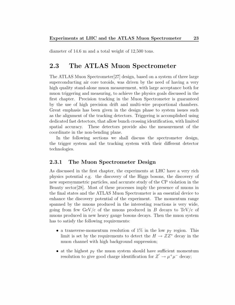
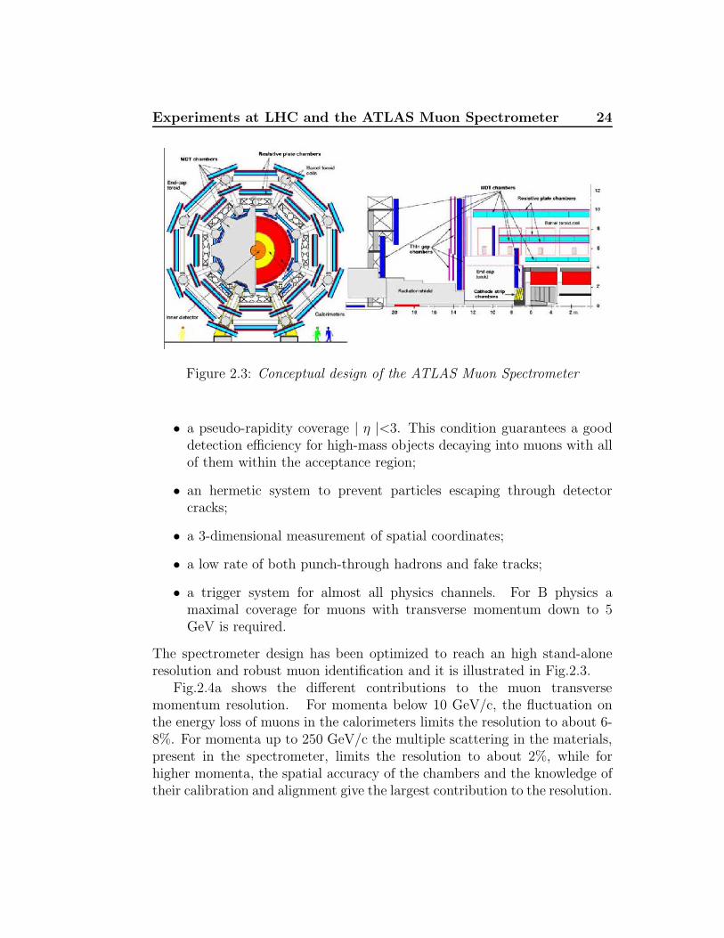
Figure 2.3: Conceptual design of the ATLAS Muon Spectrometer
• a pseudo-rapidity coverage | η |<3. This condition guarantees a gooddetection efficiency for high-mass objects decaying into muons with allof them within the acceptance region;
• an hermetic system to prevent particles escaping through detectorcracks;
• a 3-dimensional measurement of spatial coordinates;
• a low rate of both punch-through hadrons and fake tracks;
• a trigger system for almost all physics channels. For B physics amaximal coverage for muons with transverse momentum down to 5GeV is required.
The spectrometer design has been optimized to reach an high stand-aloneresolution and robust muon identification and it is illustrated in Fig.2.3.
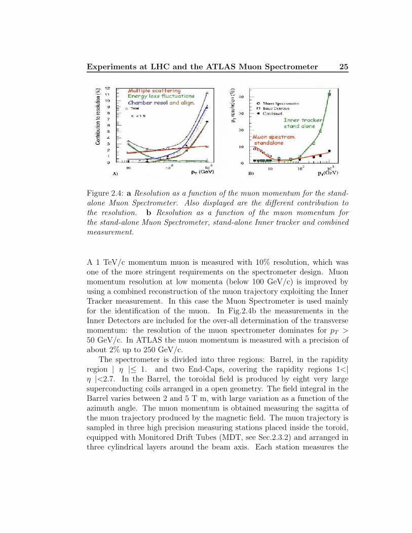
Fig.2.4a shows the different contributions to the muon transversemomentum resolution. For momenta below 10 GeV/c, the fluctuation onthe energy loss of muons in the calorimeters limits the resolution to about 6-8%. For momenta up to 250 GeV/c the multiple scattering in the materials,present in the spectrometer, limits the resolution to about 2%, while forhigher momenta, the spatial accuracy of the chambers and the knowledge oftheir calibration and alignment give the largest contribution to the resolution.
Experiments at LHC and the ATLAS Muon Spectrometer 25
Figure 2.4: a Resolution as a function of the muon momentum for the stand-alone Muon Spectrometer. Also displayed are the different contribution tothe resolution. b Resolution as a function of the muon momentum forthe stand-alone Muon Spectrometer, stand-alone Inner tracker and combinedmeasurement.
A 1 TeV/c momentum muon is measured with 10% resolution, which wasone of the more stringent requirements on the spectrometer design. Muonmomentum resolution at low momenta (below 100 GeV/c) is improved byusing a combined reconstruction of the muon trajectory exploiting the InnerTracker measurement. In this case the Muon Spectrometer is used mainlyfor the identification of the muon. In Fig.2.4b the measurements in theInner Detectors are included for the over-all determination of the transversemomentum: the resolution of the muon spectrometer dominates for pT >50 GeV/c. In ATLAS the muon momentum is measured with a precision ofabout 2% up to 250 GeV/c.
The spectrometer is divided into three regions: Barrel, in the rapidityregion | η |≤ 1. and two End-Caps, covering the rapidity regions 1<|η |<2.7. In the Barrel, the toroidal field is produced by eight very largesuperconducting coils arranged in a open geometry. The field integral in theBarrel varies between 2 and 5 T m, with large variation as a function of theazimuth angle. The muon momentum is obtained measuring the sagitta ofthe muon trajectory produced by the magnetic field. The muon trajectory issampled in three high precision measuring stations placed inside the toroid,equipped with Monitored Drift Tubes (MDT, see Sec.2.3.2) and arranged inthree cylindrical layers around the beam axis. Each station measures the
Experiments at LHC and the ATLAS Muon Spectrometer 26
muon positions with a precision of about 50 µm. In the two outer stationsof the Barrel spectrometer, specialized trigger detectors (Resistive PlateCounters, RPCs) are present. An exhaustive description of these detectorswill be presented in the next chapter. In the middle station two layers,each comprising two RPC detectors (RPC doublet), are used to form a lowpT trigger (pT >6 GeV/c). In the outer station only one layer with a RPCdoublet is used to form the high pT trigger (pT >20 GeV/c), together withthe low pT station. The RPCs measure both the bending and non-bendingcoordinate in the magnetic field. Trigger formation requires fast (< 25 ns)coincidences pointing to the interaction region both in the bending and inthe non-bending planes.
In the End-Cap regions, two identical air core toroids are placed inside thebarrel toroid with the same axis (corresponding to the beam direction). Themeasurement of the muon momentum is accomplished using three measuringstations of chambers mounted to form three big disks called ‘wheels’, normalto the beam direction and measuring the angular displacement of the muontrack when passing in the magnetic field (the toroids are placed between thefirst and the second tracking stations). In this case the toroids’ volume isnot instrumented: a sagitta measurements is not possible and a point-anglemeasurement is performed. MDT chambers are used for precise tracking inthe full angular acceptance, with the exception of the inner station wherethe region 2<| η |<2.7 is equipped with Cathode Strip Chambers (CSC,see Sec.2.3.2) which exhibit a smaller occupancy. The CSCs have spatialresolution in the range of 50 µm.
The trigger acceptance in the End-Cap is limited to | η |<2.4 where ThinGap Chambers (TGC, see sec.2.3.3) are used to provide the trigger. TheTGCs are arranged in two stations: one made of two doublets of two layerseach, used for the low pT trigger, and one made of three layers used in thehigh pT trigger in conjunction with the low pT stations. The high pT stationis placed in front of the middle precision tracking wheel and the low pT
station is behind it. The TGCs provide also the measurement of the secondcoordinate and for this reason there is a TGC layer also in the first trackingwheel.
One of the main concern comes from the background. The main source inthe ATLAS Muon Spectrometer is the large number of photons and neutrons,with energy typically below 1 MeV and 100 KeV respectively, which interactin the active volume of the tracking and trigger detectors. Typical fluencevalues in the Barrel sector are below 20 Hz/cm2 for almost all the chambers,
Experiments at LHC and the ATLAS Muon Spectrometer 27
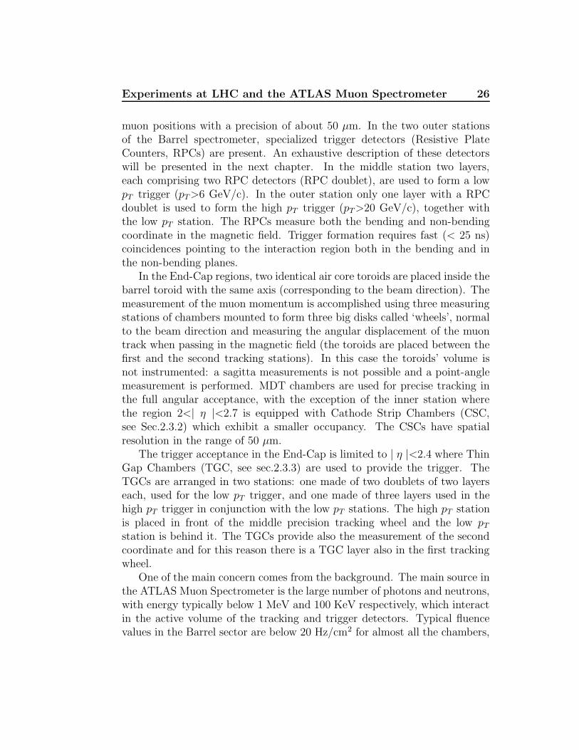
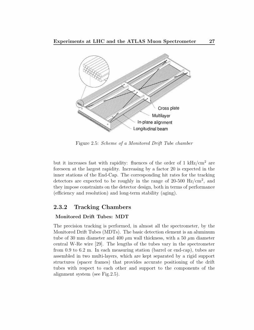
Figure 2.5: Scheme of a Monitored Drift Tube chamber
but it increases fast with rapidity: fluences of the order of 1 kHz/cm2 areforeseen at the largest rapidity. Increasing by a factor 20 is expected in theinner stations of the End-Cap. The corresponding hit rates for the trackingdetectors are expected to be roughly in the range of 20-500 Hz/cm2, andthey impose constraints on the detector design, both in terms of performance(efficiency and resolution) and long-term stability (aging).
2.3.2 Tracking Chambers
Monitored Drift Tubes: MDT
The precision tracking is performed, in almost all the spectrometer, by theMonitored Drift Tubes (MDTs). The basic detection element is an aluminumtube of 30 mm diameter and 400 µm wall thickness, with a 50 µm diametercentral W-Re wire [29]. The lengths of the tubes vary in the spectrometerfrom 0.9 to 6.2 m. In each measuring station (barrel or end-cap), tubes areassembled in two multi-layers, which are kept separated by a rigid supportstructures (spacer frames) that provides accurate positioning of the drifttubes with respect to each other and support to the components of thealignment system (see Fig.2.5).
Experiments at LHC and the ATLAS Muon Spectrometer 28
Multi-layers are formed by 3 or 4 layers of tubes, four-layer chambersbeing used in the inner stations. The mechanical accuracy in the constructionof these chambers is extremely tight to meet the momentum resolutionrequirements of the spectrometer. Using an X-Ray Tomography [30], whichmeasure the wire position with an accuracy of less than 5 µm, the precisionin wire position inside a chamber has been checked to be higher than 20 µmr.m.s. The required high pT resolution crucially depends also on the singletube resolution, defined by the operating point, the accurate knowledge ofthe calibration and the chambers’ alignment.
The MDT chambers use a mixture of Ar-CO2 (93%-7%), kept at 3bar absolute pressure, and are operated with a gas gain of 2×10⁴. Theseparameters were chosen in order to match the running condition of theexperiment: the MDTs can sustain high rates without aging [31], and withlittle sensitivity to space charge. The single tube resolution is below 100 µmfor most of the range in drift distance, and the resolution of a multi-layer isapproximately equal to 50 µm.
In order to take advantage of such tracking accuracy covering a surfaceper chamber up to 10 m2, an extremely accurate mechanical constructionis needed. Furthermore, precise monitoring of the operating conditions isrequired for best performance. Among these issues, very important is anexcellent alignment system that enables the monitoring of the position of thedifferent chambers in the spectrometer with a precision higher than 30 µm.Regarding this system, the aluminum frame supporting the multi-layers isequipped with RASNIK [32] optical straightness monitors. These monitorsare formed by three elements along a view line: a laser that illuminates acoded target mask at one end, a lens in the middle and a CCD (ChargedCoupled Device)sensors at the other end. This system provides a veryaccurate measurement of the relative alignment of three objects (1 µm r.m.s.)and is used both for checking the chamber deformation (in-plane alignment),and the relative displacement of different chamber (projective alignment).The chambers are also equipped with temperature monitors (in order tocorrect for the thermal expansion of the tubes, and for the temperature ofthe gas), and with magnetic field sensors, in order to predict the E×B effecton the drift time.
Experiments at LHC and the ATLAS Muon Spectrometer 29
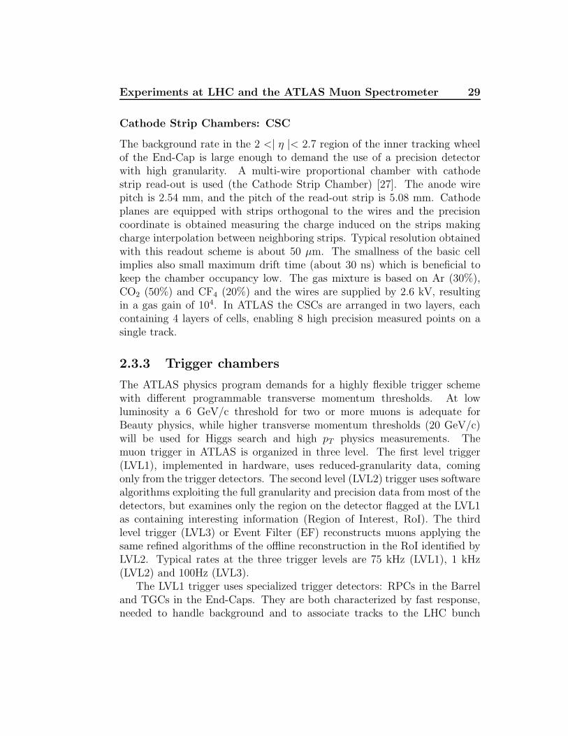
Cathode Strip Chambers: CSC
The background rate in the 2 <| η |< 2.7 region of the inner tracking wheelof the End-Cap is large enough to demand the use of a precision detectorwith high granularity. A multi-wire proportional chamber with cathodestrip read-out is used (the Cathode Strip Chamber) [27]. The anode wirepitch is 2.54 mm, and the pitch of the read-out strip is 5.08 mm. Cathodeplanes are equipped with strips orthogonal to the wires and the precisioncoordinate is obtained measuring the charge induced on the strips makingcharge interpolation between neighboring strips. Typical resolution obtainedwith this readout scheme is about 50 µm. The smallness of the basic cellimplies also small maximum drift time (about 30 ns) which is beneficial tokeep the chamber occupancy low. The gas mixture is based on Ar (30%),CO2 (50%) and CF4 (20%) and the wires are supplied by 2.6 kV, resultingin a gas gain of 104. In ATLAS the CSCs are arranged in two layers, eachcontaining 4 layers of cells, enabling 8 high precision measured points on asingle track.
2.3.3 Trigger chambers
The ATLAS physics program demands for a highly flexible trigger schemewith different programmable transverse momentum thresholds. At lowluminosity a 6 GeV/c threshold for two or more muons is adequate forBeauty physics, while higher transverse momentum thresholds (20 GeV/c)will be used for Higgs search and high pT physics measurements. Themuon trigger in ATLAS is organized in three level. The first level trigger(LVL1), implemented in hardware, uses reduced-granularity data, comingonly from the trigger detectors. The second level (LVL2) trigger uses softwarealgorithms exploiting the full granularity and precision data from most of thedetectors, but examines only the region on the detector flagged at the LVL1as containing interesting information (Region of Interest, RoI). The thirdlevel trigger (LVL3) or Event Filter (EF) reconstructs muons applying thesame refined algorithms of the offline reconstruction in the RoI identified byLVL2. Typical rates at the three trigger levels are 75 kHz (LVL1), 1 kHz(LVL2) and 100Hz (LVL3).
The LVL1 trigger uses specialized trigger detectors: RPCs in the Barreland TGCs in the End-Caps. They are both characterized by fast response,needed to handle background and to associate tracks to the LHC bunch
Experiments at LHC and the ATLAS Muon Spectrometer 30
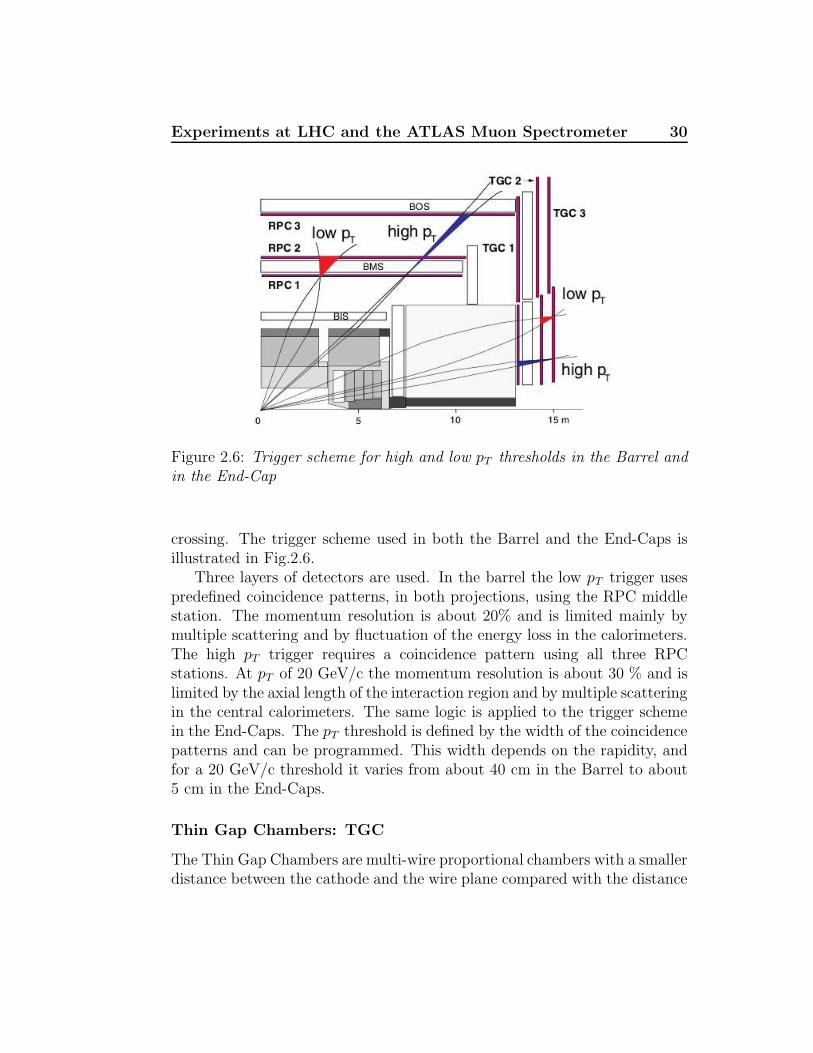
Figure 2.6: Trigger scheme for high and low pT thresholds in the Barrel andin the End-Cap
crossing. The trigger scheme used in both the Barrel and the End-Caps isillustrated in Fig.2.6.
Three layers of detectors are used. In the barrel the low pT trigger usespredefined coincidence patterns, in both projections, using the RPC middlestation. The momentum resolution is about 20% and is limited mainly bymultiple scattering and by fluctuation of the energy loss in the calorimeters.The high pT trigger requires a coincidence pattern using all three RPCstations. At pT of 20 GeV/c the momentum resolution is about 30 % and islimited by the axial length of the interaction region and by multiple scatteringin the central calorimeters. The same logic is applied to the trigger schemein the End-Caps. The pT threshold is defined by the width of the coincidencepatterns and can be programmed. This width depends on the rapidity, andfor a 20 GeV/c threshold it varies from about 40 cm in the Barrel to about5 cm in the End-Caps.
Thin Gap Chambers: TGC
The Thin Gap Chambers are multi-wire proportional chambers with a smallerdistance between the cathode and the wire plane compared with the distance
Experiments at LHC and the ATLAS Muon Spectrometer 31
between wires [33]. In fact, the distance between the cathode and the wiresis 1.4 mm compared with the wires pitch that is 1.8 mm., while the wirediameter is 50 µm.
The gas mixture is 50% CO2 and 45% n-pentane, which results in a highlyquenching gas mixture that permits the operation in saturated avalanchemode (see next chapter for detailed description of the gas detectors operationmodes). Due to this operation mode, these detectors are not very sensitiveto small mechanical deformations, which is very important for large detectoras ATLAS [34].The saturated mode has also two more advantage: the signalproduced by a minimum ionizing particle has only a small dependence onthe incident angle up to angles of 40 degrees; the tails of the pulse-heightdistribution contain only a small fraction of the pulse-heights (less than 2%).The chambers operate at high voltage of about 3 kV. The operating conditionand the electric field configuration provide for a short drift time (< 30 ns),enabling a good time resolution. The readout of the signal is done both fromthe wires (which are grounded together in a variable number, according tothe desired trigger granularity as a function of the pseudo-rapidity) and fromthe pick-up strips plane placed on the cathode. The wires and the stripsare perpendicular to each other enabling the measurement of the orthogonalcoordinates, however, only the wire signal are used in the trigger logic.
Test performed at high rate have shown single-plane time resolution ofabout 4 ns with 98% efficiency, providing a trigger efficiency of 99.6% [35].
Resistive Plate Counters: RPC
The RPC are gaseous detectors providing a typical space-time resolution of1 cm × 1 ns with digital readout. The active element of the RPC unit isa narrow gas gap formed by two parallel resistive Bakelite plates, separatedby insulating spacers. The primary ionization electrons are multiplied inavalanches by a high, uniform electric field of typically 5 kV/mm. The gasmixture used has been selected in order to allow operating in saturatedavalanche mode (see next chapter for the gas detector operation modedescription) and is composed of three gases: 94.7% C2H2F4, 5% C4H10,0.3% SF6. Tetrafluoroethane (C2H2F4) has been chosen as main componentsince, in addition to satisfy safety requirements, exhibits moderately highprimary ionization at low operating voltage. Moreover, the mixture containsisobutane (C4H10) as photons quencher and SF6, in order to reduce theamount of delivered charge and inhibit the streamer development.
Experiments at LHC and the ATLAS Muon Spectrometer 32
Amplification in avalanche mode produces pulses of typically 0.5 pC.Signals are readout via capacitive coupling by metal strips on both sidesof the detectors. In ATLAS, RPC are mounted on MDTs with a mechanicalstructure that fix the relative position between RPCs and MDTs. In onereadout plane strips (η strips) are parallel to the MDT wires and providethe bending view, while in the other plane strips (φ strips) are orthogonalto the MTD wires, providing the second-coordinate measurement which isalso required for the pattern recognition. RPC detectors will be extensivelydescribed in the next chapter.
Chapter 3
Resistive Plate Counters
3.1 Introduction
Resistive Plate Counters (RPC) have been developed in 1981 by R. Santonicoand R. Cardarelli [36, 37]. They are gaseous resistive parallel plate detectorswith a time resolution of ∼ 1 ns, consequently attractive for triggering andTime-Of-Flight applications.
Their main advantages, compared to other technologies, consist in theirrobustness, construction simplicity and relatively low cost of the industrialproduction. They are ideal to cover large areas up to few thousand squaremeters.
RPCs where originally used in streamer mode operation [38], providinglarge electrical signals, requiring low gain read-out electronics and notstringent gap uniformity. However, high rate applications and detector agingissues made the operation in avalanche [38] mode necessary. This was possiblethanks to the use of new highly quenching C2H2F2-based gas mixture insteadof the traditional Ar-based mixture and to the development of high gain read-out electronics.
Streamers generation dynamics is difficult to study and the avalanchemode operation should open up the possibility of implementing detailedsimulations, thus allowing for a better understanding of the physics processesin the RPC. In this chapter we will discuss RPC physics structure andoperation.
Resistive Plate Counter 34
Figure 3.1: Schematic image of the RPC.
3.2 Resistive Plate Chambers
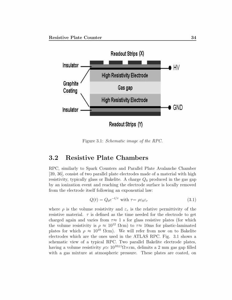
RPC, similarly to Spark Counters and Parallel Plate Avalanche Chamber[39, 36], consist of two parallel plate electrodes made of a material with highresistivity, typically glass or Bakelite. A charge Q0 produced in the gas gapby an ionization event and reaching the electrode surface is locally removedfrom the electrode itself following an exponential law:
Q(t) = Q0e−t/τ with τ= ρε0εr (3.1)
where ρ is the volume resistivity and εr is the relative permittivity of theresistive material. τ is defined as the time needed for the electrode to getcharged again and varies from τ≈ 1 s for glass resistive plates (for whichthe volume resistivity is ρ ≈ 1012 Ωcm) to τ≈ 10ms for plastic-laminatedplates for which ρ ≈ 1010 Ωcm). We will refer from now on to Bakeliteelectrodes which are the ones used in the ATLAS RPC. Fig. 3.1 shows aschematic view of a typical RPC. Two parallel Bakelite electrode plates,having a volume resistivity ρ' 1010±1Ω×cm, delimits a 2 mm gas gap filledwith a gas mixture at atmospheric pressure. These plates are coated, on
Resistive Plate Counter 35
the external side, with a thin graphite layer with a surface resistivity rangingfrom 100 to 300 kΩ/. The graphite layer allows to uniformly apply the highvoltage to the electrodes without screening the avalanche signal induced onmetal strip readout panels. The readout panels are segmented into stripsand simply pressed on the external electrode surface. The readout strips areon both sides of the gap and arranged in perpendicular directions in one sidewith respect to the other, allowing to measure the x- and y-coordinate ofthe ionizing particle. Strip panels are separated from the graphite coatingby an isolating PET foil. Moreover, the assembled RPC gas volume is filledwith linseed oil, which is then slowly taken out. The resulting effect is thedeposition of a thin layer of polymerized oil [36] which smooth both innerBakelite surfaces. This is done in order to strongly reduce the detector darkcurrent and noise counting rate.
The fundamental processes underlying RPCs are well known: a chargedparticle produces free charge carriers in the gas, which drift towards theanode and are multiplied by an uniform electric field induced by an externalhigh voltage applied to the electrode plates. The propagation of the growingnumber of charges induces an electric signal on the read-out strips, which isamplified and discriminated by the front-end electronics.
In the following sections, we will briefly describe the physics processes thatproduce a signal in the RPC detectors and, in general, in a gas detector, thetransport properties of electrons in a gas when an electric field is applied,the electron avalanche generation and related phenomena. Finally, we willillustrate the mechanism of the signal induction by the avalanche.
3.3 Particle Energy Loss in the Matter
A charged particle crossing a material will loose energy by Coloumbianinelastic scattering with atomic electrons of the material. If the impactparameter is large compared to the size of the atom (a distant collision), theatom will react ‘as a whole’to the variable electromagnetic field of the chargedparticle. The result can be excitation or ionization of the atom with theemission of an electron with small energy. Instead, if the impact parameteris of the order of the atomic dimension (a close collision), the interactioninvolves one of the atomic electrons. As a consequence, the electron is ejectedfrom the atom with considerable energy (knock-on electrons or delta rays).If the collision energy is sufficiently large we can treat all close collision by
Resistive Plate Counter 36
considering the atomic electrons as free particles.The total energy lost by the charged particle is the sum of the two
contributions: close and distant collisions. For distant collisions, it isimportant to take into account the binding energy of the electrons to theatoms, this mean to consider the average ionization energy I [MeV] ofthe atom [40]. For close collision is necessary to consider the maximumtransferable energy Emax, applying energy and momentum conservationprinciples. These leads to the following relation for the maximum kineticenergy transferable to a free electron by a particle of mass m and velocityβ(in units of c)[41]:
Emax =2mec
2β2γ2
1 + 2me
msqrt1 + β2γ2 + (me
m)2
(3.2)
which for relativistic particles becomes:
Emax ≈ 2mec2β2γ2 (3.3)
The two contributions to the total energy loss by a heavy particles can bewritten as:
−1
ρ
dE
dx
∣
∣
∣
coll=
k
β2
Zz2
A
[
ln2mec
2β2γ2Emax
I2− 2β2 − δ
]
(3.4)
where:
1ρ
dEdx
∣
∣
∣
coll- the average energy loss [MeV cm2/g],
k - a constant defined by k=2π Nare2mec
2 [= 0.1535 MeV cm2/g],
ρ, Z, A - the density, atomic number and atomic weight of the absorbingmaterial,
re - the classic electron radius re= 2.817× 10⁻¹³ cm,
me - the electron mass,
Na - the Avogadro’s number,
z, β - the charge and the velocity of the particle in units of electroncharge and c respectively,
γ - is given by 1/√
1 − β2 as usual.
Resistive Plate Counter 37
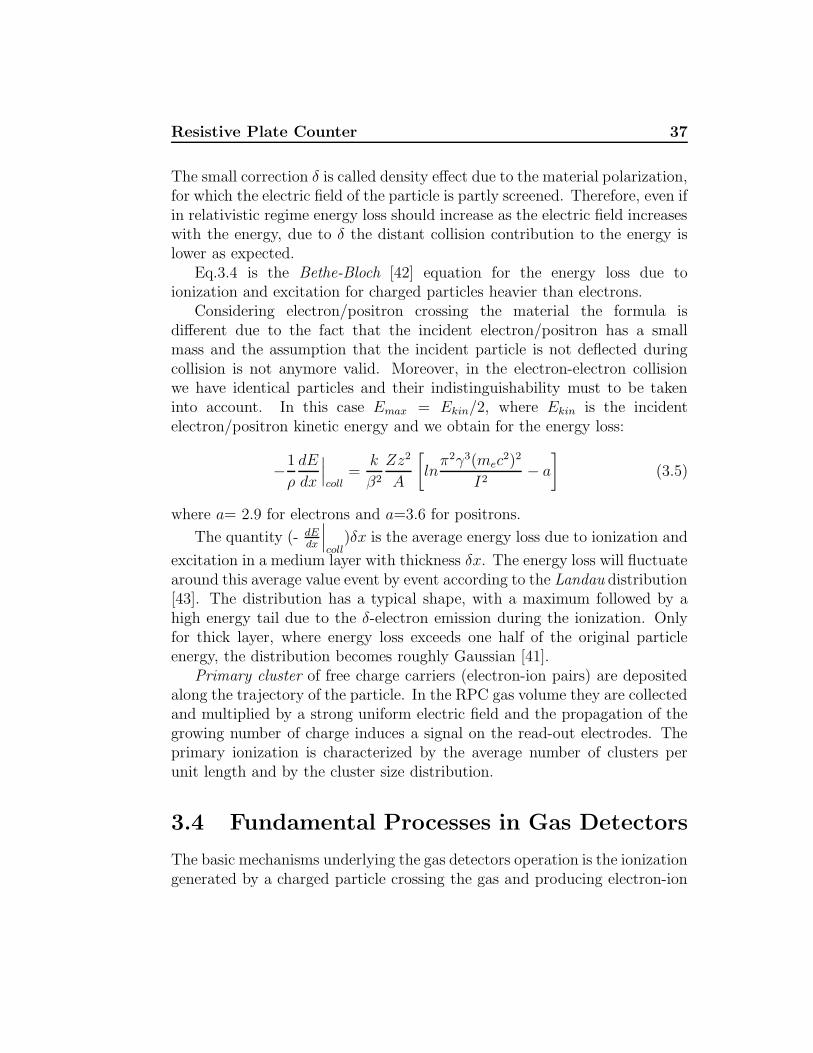
The small correction δ is called density effect due to the material polarization,for which the electric field of the particle is partly screened. Therefore, even ifin relativistic regime energy loss should increase as the electric field increaseswith the energy, due to δ the distant collision contribution to the energy islower as expected.
Eq.3.4 is the Bethe-Bloch [42] equation for the energy loss due toionization and excitation for charged particles heavier than electrons.
Considering electron/positron crossing the material the formula isdifferent due to the fact that the incident electron/positron has a smallmass and the assumption that the incident particle is not deflected duringcollision is not anymore valid. Moreover, in the electron-electron collisionwe have identical particles and their indistinguishability must to be takeninto account. In this case Emax = Ekin/2, where Ekin is the incidentelectron/positron kinetic energy and we obtain for the energy loss:
−1
ρ
dE
dx
∣
∣
∣
coll=
k
β2
Zz2
A
[
lnπ2γ3(mec
2)2
I2− a
]
(3.5)
where a= 2.9 for electrons and a=3.6 for positrons.
The quantity (- dEdx
∣
∣
∣
coll)δx is the average energy loss due to ionization and
excitation in a medium layer with thickness δx. The energy loss will fluctuatearound this average value event by event according to the Landau distribution[43]. The distribution has a typical shape, with a maximum followed by ahigh energy tail due to the δ-electron emission during the ionization. Onlyfor thick layer, where energy loss exceeds one half of the original particleenergy, the distribution becomes roughly Gaussian [41].
Primary cluster of free charge carriers (electron-ion pairs) are depositedalong the trajectory of the particle. In the RPC gas volume they are collectedand multiplied by a strong uniform electric field and the propagation of thegrowing number of charge induces a signal on the read-out electrodes. Theprimary ionization is characterized by the average number of clusters perunit length and by the cluster size distribution.
3.4 Fundamental Processes in Gas Detectors
The basic mechanisms underlying the gas detectors operation is the ionizationgenerated by a charged particle crossing the gas and producing electron-ion
Resistive Plate Counter 38
pairs (primary charge). In the following sections we consider the behavior offree electrons in a gas, with an electric field applied, and how they give riseto a detectable signal.
3.4.1 Electrons Diffusion
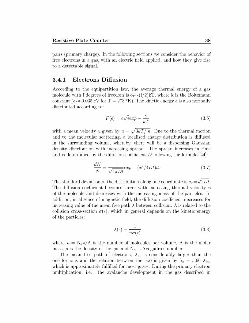
According to the equipartition law, the average thermal energy of a gasmolecule with f degrees of freedom is εT∼(f/2)kT, where k is the Boltzmannconstant (εT≈0.035 eV for T = 273 oK). The kinetic energy ε is also normallydistributed according to:
F (ε) = c√
εexp − ε
kT(3.6)
with a mean velocity u given by u =√
3kT/m. Due to the thermal motionand to the molecular scattering, a localized charge distribution is diffusedin the surrounding volume, whereby, there will be a dispersing Gaussiandensity distribution with increasing spread. The spread increases in timeand is determined by the diffusion coefficient D following the formula [44]:
dN
N=
1√4πDt
exp − (x2/4Dt)dx (3.7)
The standard deviation of the distribution along one coordinate is σx=√
2Dt.The diffusion coefficient becomes larger with increasing thermal velocity uof the molecule and decreases with the increasing mass of the particles. Inaddition, in absence of magnetic field, the diffusion coefficient decreases forincreasing value of the mean free path λ between collision. λ is related to thecollision cross-section σ(ε), which in general depends on the kinetic energyof the particles:
λ(ε) =1
nσ(ε)(3.8)
where n = Naρ/A is the number of molecules per volume, A is the molarmass, ρ is the density of the gas and Na is Avogadro’s number.
The mean free path of electrons, λe, is considerably larger than theone for ions and the relation between the two is given by λe = 5.66 λion
which is approximately fulfilled for most gases. During the primary electronmultiplication, i.e. the avalanche development in the gas described in
Resistive Plate Counter 39
sec.3.4.4, the charge distribution diffuse laterally and longitudinally due tothe electrons diffusion. In RPC counters the avalanche spread, before chargecollection occurs, is of about few millimeters.
3.4.2 Electron Drift
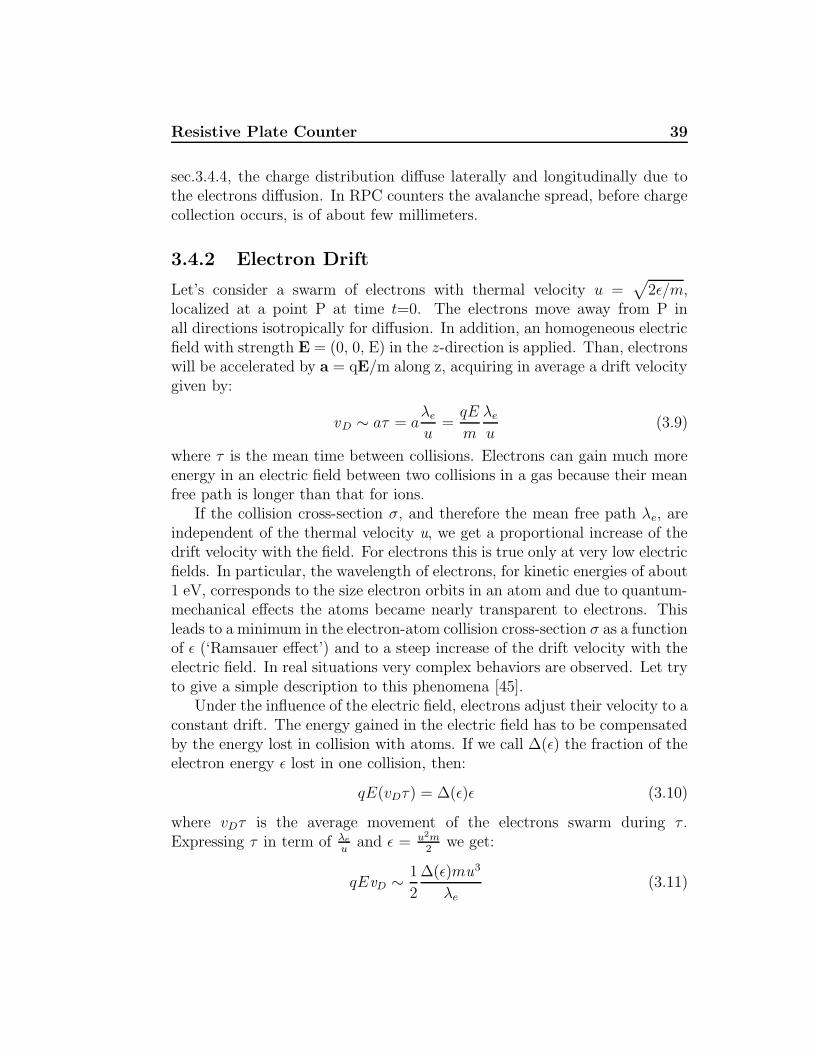
Let’s consider a swarm of electrons with thermal velocity u =√
2ε/m,localized at a point P at time t=0. The electrons move away from P inall directions isotropically for diffusion. In addition, an homogeneous electricfield with strength E = (0, 0, E) in the z-direction is applied. Than, electronswill be accelerated by a = qE/m along z, acquiring in average a drift velocitygiven by:
vD ∼ aτ = aλe
u=
qE
m
λe
u(3.9)
where τ is the mean time between collisions. Electrons can gain much moreenergy in an electric field between two collisions in a gas because their meanfree path is longer than that for ions.
If the collision cross-section σ, and therefore the mean free path λe, areindependent of the thermal velocity u, we get a proportional increase of thedrift velocity with the field. For electrons this is true only at very low electricfields. In particular, the wavelength of electrons, for kinetic energies of about1 eV, corresponds to the size electron orbits in an atom and due to quantum-mechanical effects the atoms became nearly transparent to electrons. Thisleads to a minimum in the electron-atom collision cross-section σ as a functionof ε (‘Ramsauer effect’) and to a steep increase of the drift velocity with theelectric field. In real situations very complex behaviors are observed. Let tryto give a simple description to this phenomena [45].
Under the influence of the electric field, electrons adjust their velocity to aconstant drift. The energy gained in the electric field has to be compensatedby the energy lost in collision with atoms. If we call ∆(ε) the fraction of theelectron energy ε lost in one collision, then:
qE(vDτ) = ∆(ε)ε (3.10)
where vDτ is the average movement of the electrons swarm during τ .Expressing τ in term of λe
uand ε = u2m
2we get:
qEvD ∼ 1
2
∆(ε)mu3
λe
(3.11)
Resistive Plate Counter 40
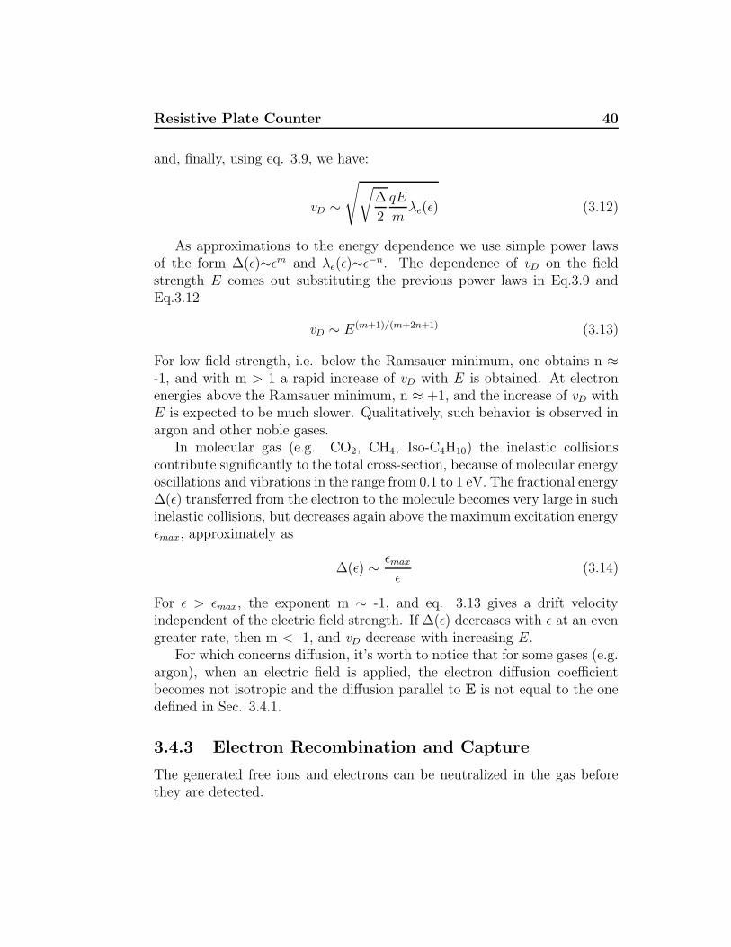
and, finally, using eq. 3.9, we have:
vD ∼
√
√
∆
2
qE
mλe(ε) (3.12)
As approximations to the energy dependence we use simple power lawsof the form ∆(ε)∼εm and λe(ε)∼ε−n. The dependence of vD on the fieldstrength E comes out substituting the previous power laws in Eq.3.9 andEq.3.12
vD ∼ E(m+1)/(m+2n+1) (3.13)
For low field strength, i.e. below the Ramsauer minimum, one obtains n ≈-1, and with m > 1 a rapid increase of vD with E is obtained. At electronenergies above the Ramsauer minimum, n ≈ +1, and the increase of vD withE is expected to be much slower. Qualitatively, such behavior is observed inargon and other noble gases.
In molecular gas (e.g. CO2, CH4, Iso-C4H10) the inelastic collisionscontribute significantly to the total cross-section, because of molecular energyoscillations and vibrations in the range from 0.1 to 1 eV. The fractional energy∆(ε) transferred from the electron to the molecule becomes very large in suchinelastic collisions, but decreases again above the maximum excitation energyεmax, approximately as
∆(ε) ∼ εmax
ε(3.14)
For ε > εmax, the exponent m ∼ -1, and eq. 3.13 gives a drift velocityindependent of the electric field strength. If ∆(ε) decreases with ε at an evengreater rate, then m < -1, and vD decrease with increasing E.
For which concerns diffusion, it’s worth to notice that for some gases (e.g.argon), when an electric field is applied, the electron diffusion coefficientbecomes not isotropic and the diffusion parallel to E is not equal to the onedefined in Sec. 3.4.1.
3.4.3 Electron Recombination and Capture
The generated free ions and electrons can be neutralized in the gas beforethey are detected.
Resistive Plate Counter 41
Recombination process of positive ions with negative ions or withelectrons can occur. The density decrease of positive ions, n+, with timecan be described by the relation -dn+/dt=αn+n−, where n− is the density ofthe negatively charged particles and α is called ‘recombination coefficient’. Ingases, like O2 and CO2, α can reach a value of 10−6 cm3/s for recombinationwith negative ions, and values up to 10−7 cm3/s for recombination withelectrons.
Free electrons are removed from the gas also by the molecular capture.Gas molecules with several atoms are able to capture electrons of low (eV)energy and produce negative ions of lower mobility. The probability pa thatthis happens during one collision is negligibly small for noble gases and forN2, H2 and CH4, but not for electronegative gases like O2, Cl−2, NH3 andH2O. The mean time for electron capture is given by ta= 1/(pans) where ns
the number of collisions per unit time. For strongly electronegative gases atnormal conditions ta can be as small as 5 ns.
If an electric field is applied, the kinetic energy ε of the electrons increasesand the probability pa(ε) for electron capture varies with energy. In this casethe mean free path of electrons relative to electron capture is
λa =vD
pans(3.15)
Considering this capture effect, it comes out that the free electrons intensityin the gas (Ie0) is reduced with the drift distance following an exponentiallaw:
Ie = Ie0exp(−βx) (3.16)
where β is named “attachment coefficient ”, which depends strongly on theenergy of the ionizing particle and on the presence of an electric field. Asimilar strong dependence, but of opposite sign, is related to the electronavalanche development which is the topic of the next section.
3.4.4 Electron Multiplication
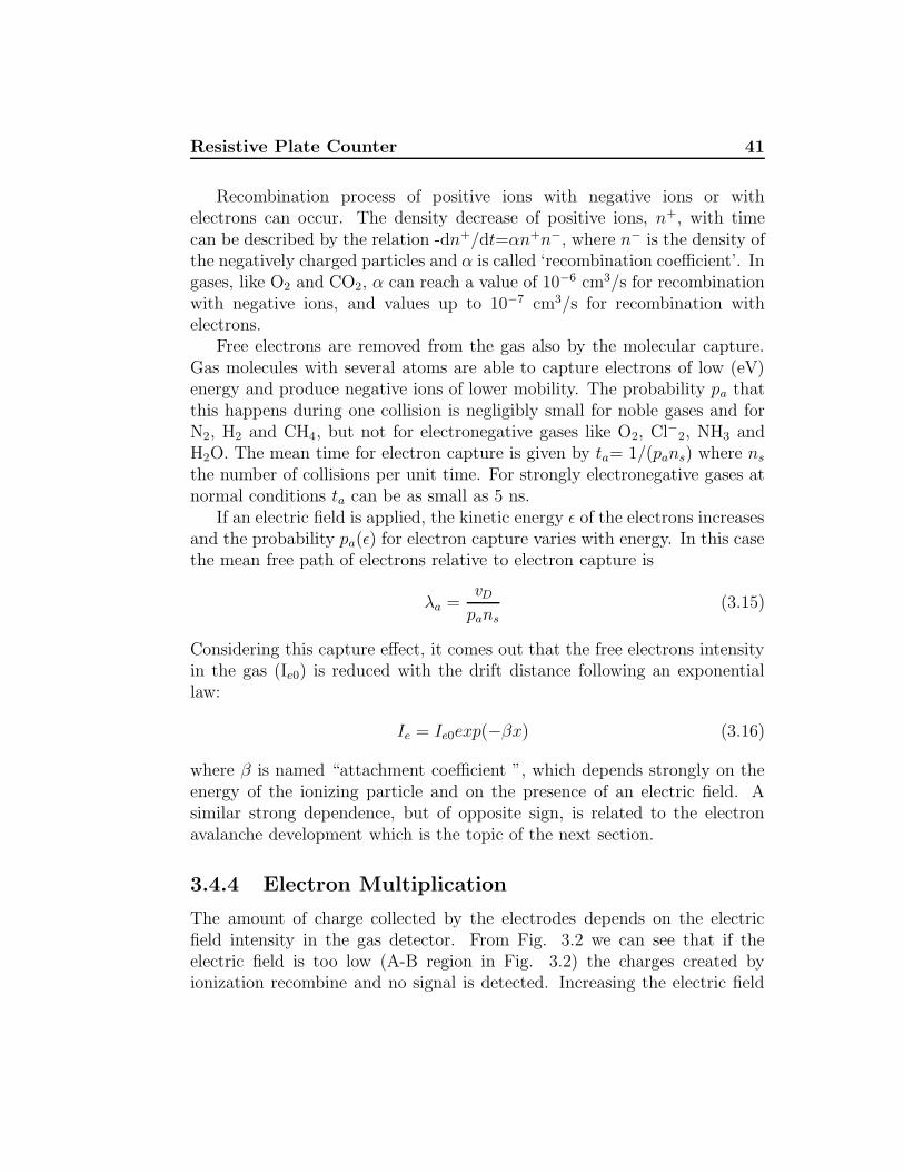
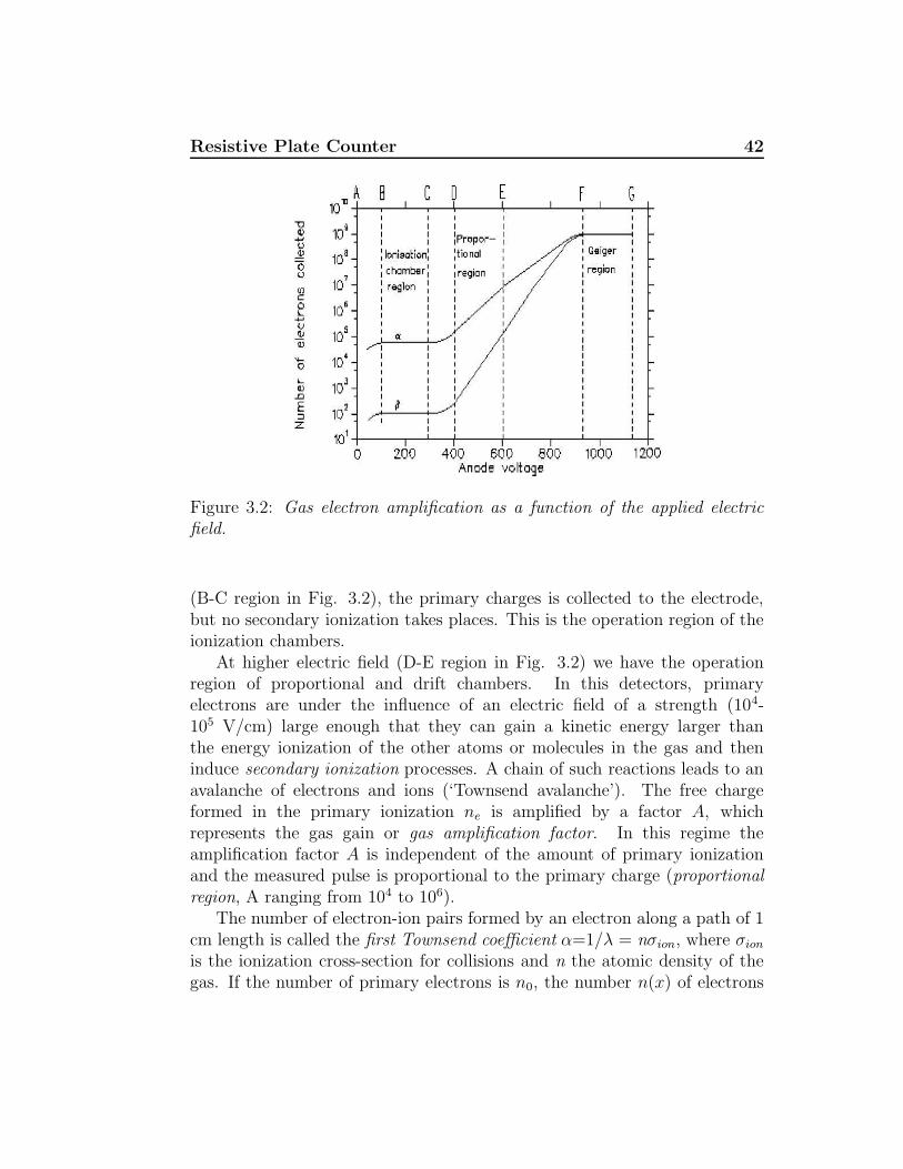
The amount of charge collected by the electrodes depends on the electricfield intensity in the gas detector. From Fig. 3.2 we can see that if theelectric field is too low (A-B region in Fig. 3.2) the charges created byionization recombine and no signal is detected. Increasing the electric field
Resistive Plate Counter 42
Figure 3.2: Gas electron amplification as a function of the applied electricfield.
(B-C region in Fig. 3.2), the primary charges is collected to the electrode,but no secondary ionization takes places. This is the operation region of theionization chambers.
At higher electric field (D-E region in Fig. 3.2) we have the operationregion of proportional and drift chambers. In this detectors, primaryelectrons are under the influence of an electric field of a strength (104-105 V/cm) large enough that they can gain a kinetic energy larger thanthe energy ionization of the other atoms or molecules in the gas and theninduce secondary ionization processes. A chain of such reactions leads to anavalanche of electrons and ions (‘Townsend avalanche’). The free chargeformed in the primary ionization ne is amplified by a factor A, whichrepresents the gas gain or gas amplification factor. In this regime theamplification factor A is independent of the amount of primary ionizationand the measured pulse is proportional to the primary charge (proportionalregion, A ranging from 104 to 106).
The number of electron-ion pairs formed by an electron along a path of 1cm length is called the first Townsend coefficient α=1/λ = nσion, where σion
is the ionization cross-section for collisions and n the atomic density of thegas. If the number of primary electrons is n0, the number n(x) of electrons
Resistive Plate Counter 43
after a path length x is obtained as:
n(x) = n0exp(αx) (3.17)
to be compared with Eq. 3.16.Photons originated by the atomic de-excitation, during the multiplication
process, give rise to secondary phenomena. They produce, in fact, photo-electrons in the gas or extracted from the electrodes. This phenomenonis quantified by the second Townsend coefficient γ, i.e. the probabilityto have a generated photo-electron for each electron belonging to theavalanche. If an avalanche started by n0 primary electrons, n0A electronsare produced in secondary ionization and, at the same time, (n0A)γphoto-electron are produced in connection with ultraviolet photons fromradiative processes. These photoelectrons are then amplified producingn0A
2γ secondary electrons. In this avalanche n0A2γ2 photoelectrons are
formed again, and n0A3γ2 electrons are liberated, etc. Adding the number
of electrons from the sequential steps, one obtains:
n0Aγ = n0
∑
n>0
(Aγ)n =n0A
1 − Aγ(3.18)
This Aγ is the gas amplification factor including the energy transfer byphotons. If Aγ→1 and quenching mechanism are nor present, than thegas gain became infinite. This region of operation is called Geiger-Mullerregion (F-G region in Fig. 3.2). In the Geiger-Muller region the avalanchespreads over the whole counter and leads to a complete discharge. The gasamplification in this case is A∼108-1010 and the signal output no longerdepends on the primary ionization.
In a detector not operating in Geiger-Muller mode, the propagation of theultraviolet photons is prevented, in order to avoid the discharge, by addingquenching gas which absorbs energetic photons. Usually this is an organic gaslike isobutane (C4H10) that is efficient in absorbing photons in the relevantenergy ranges.
In the region between the proportional and the Geiger-Muller regime thereis still a limited proportionality (E-F region in Fig. 3.2) between primaryionization and total liberated charge. This region is given approximatelyby αx∼20 or A∼108. RPC detectors in avalanche mode, as the ones inATLAS and CMS muon spectrometers, operate in this region (“saturatedavalanche”regime) that is characterized by space charge phenomena and gas
Resistive Plate Counter 44
gain increasing only linearly with the external field. The space charge effectsare mainly due to local electric field deformation caused by avalanche chargecarriers. In fact, at the tip and tail of the charge distribution the electricfields become higher than the applied one. Instead, in the avalanche centerthe field is lower. This electric field distortion modifies the avalanche growthand secondary and non-linear effects can take place.
3.5 Signal Readout in RPC
We will start considering a single electron of charge -e moving inside the gasvolume under the influence of a constant electric field and we will evaluatethe electric signal induced on an external conductive plane.
3.5.1 Ramo’s theorem: the ‘k factor’
A charge q(t) moving with velocity vD(t) induces an instantaneous currenti(t) according to the formula (Ramo’s theorem [46]):
i(t) = q(t)vD(t)Ew
Vw, (3.19)
where Ew is the so called weightingfield, which is obtained by applyingVw=1 V at the pick-up strip and grounding all the other electrodes. Itis important to notice that the weighting field is a fictitious field, differentfrom the real electric field, which determines the drift velocity vD(t) of theelectron. It turns out that in the RPC detector the readout plane weightingfield is given by the equation:
gEw
Vw= k =
εrg
εrg + 2d(3.20)
where d is the electrode plate thickness, g the gas gap thickness and εr is theelectrode relative dielectric permittivity. Equation 3.20 shows that, due tothe presence of the high resistivity electrodes, the induced signal is reducedby the factor k (ranging from 0.5 to 0.7 for εr ranging from 5 to 10).
In the RPC detector the electron drift velocity is uniform and the inducedcurrent is constant until the electron is collected by the electrode. In the realdevice the readout plane consists of metal strip of 3 cm pitch as in figure3.3. Just underneath the strip the electric field is quite uniform and the
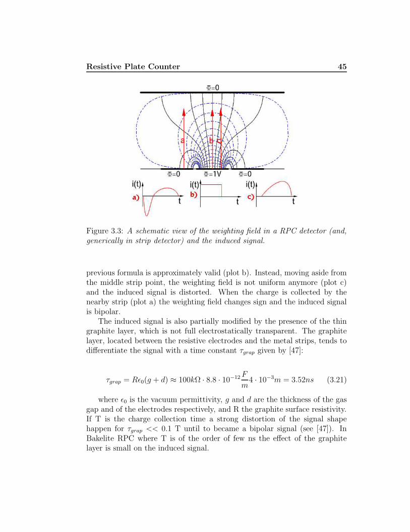
Resistive Plate Counter 45
Figure 3.3: A schematic view of the weighting field in a RPC detector (and,generically in strip detector) and the induced signal.
previous formula is approximately valid (plot b). Instead, moving aside fromthe middle strip point, the weighting field is not uniform anymore (plot c)and the induced signal is distorted. When the charge is collected by thenearby strip (plot a) the weighting field changes sign and the induced signalis bipolar.
The induced signal is also partially modified by the presence of the thingraphite layer, which is not full electrostatically transparent. The graphitelayer, located between the resistive electrodes and the metal strips, tends todifferentiate the signal with a time constant τgrap given by [47]:
τgrap = Rε0(g + d) ≈ 100kΩ · 8.8 · 10−12 F
m4 · 10−3m = 3.52ns (3.21)
where ε0 is the vacuum permittivity, g and d are the thickness of the gasgap and of the electrodes respectively, and R the graphite surface resistivity.If T is the charge collection time a strong distortion of the signal shapehappen for τgrap << 0.1 T until to became a bipolar signal (see [47]). InBakelite RPC where T is of the order of few ns the effect of the graphitelayer is small on the induced signal.
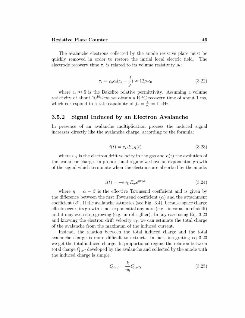
Resistive Plate Counter 46
The avalanche electrons collected by the anode resistive plate must bequickly removed in order to restore the initial local electric field. Theelectrode recovery time τr is related to its volume resistivity ρb:
τr = ρbε0(εb +d
g) ≈ 12ρbε0 (3.22)
where εb ≈ 5 is the Bakelite relative permittivity. Assuming a volumeresistivity of about 1010Ωcm we obtain a RPC recovery time of about 1 ms,which correspond to a rate capability of fr = 1
τr= 1 kHz.
3.5.2 Signal Induced by an Electron Avalanche
In presence of an avalanche multiplication process the induced signalincreases directly like the avalanche charge, according to the formula:
i(t) = vDEwq(t) (3.23)
where vD is the electron drift velocity in the gas and q(t) the evolution ofthe avalanche charge. In proportional regime we have an exponential growthof the signal which terminate when the electrons are absorbed by the anode:
i(t) = −evDEweηvDt (3.24)
where η = α − β is the effective Townsend coefficient and is given bythe difference between the first Townsend coefficient (α) and the attachmentcoefficient (β). If the avalanche saturates (see Fig. 3.4), because space chargeeffects occur, its growth is not exponential anymore (e.g. linear as in ref aielli)and it may even stop growing (e.g. in ref riglher). In any case using Eq. 3.23and knowing the electron drift velocity vD we can estimate the total chargeof the avalanche from the maximum of the induced current.
Instead, the relation between the total induced charge and the totalavalanche charge is more difficult to extract. In fact, integrating eq 3.23we get the total induced charge. In proportional regime the relation betweentotal charge Qcoll developed by the avalanche and collected by the anode withthe induced charge is simple:
Qind =k
ηgQcoll, (3.25)
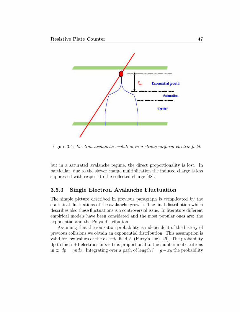
Resistive Plate Counter 47
Figure 3.4: Electron avalanche evolution in a strong uniform electric field.
but in a saturated avalanche regime, the direct proportionality is lost. Inparticular, due to the slower charge multiplication the induced charge is lesssuppressed with respect to the collected charge [48].
3.5.3 Single Electron Avalanche Fluctuation
The simple picture described in previous paragraph is complicated by thestatistical fluctuations of the avalanche growth. The final distribution whichdescribes also these fluctuations is a controversial issue. In literature differentempirical models have been considered and the most popular ones are: theexponential and the Polya distribution.
Assuming that the ionization probability is independent of the history ofprevious collisions we obtain an exponential distribution. This assumption isvalid for low values of the electric field E (Furry’s law) [49]. The probabilitydp to find n+1 electrons in x+dx is proportional to the number n of electronsin x: dp = ηndx. Integrating over a path of length l = g−x0 the probability
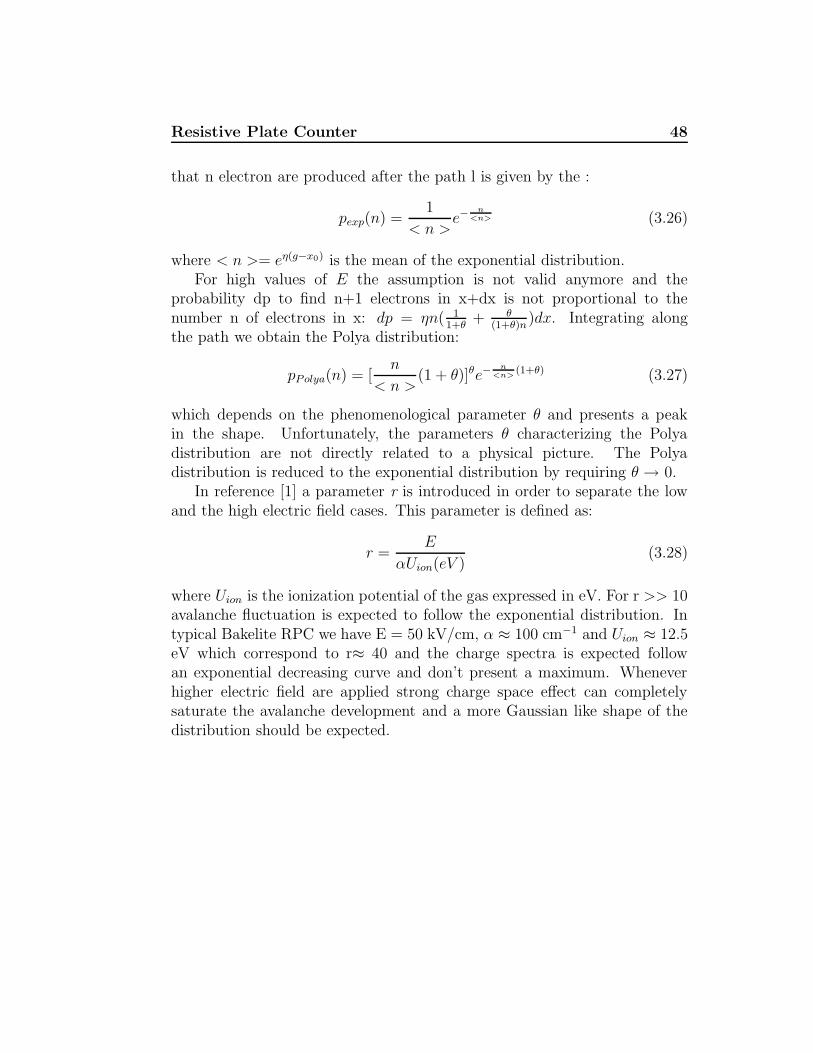
Resistive Plate Counter 48
that n electron are produced after the path l is given by the :
pexp(n) =1
< n >e−
n<n> (3.26)
where < n >= eη(g−x0) is the mean of the exponential distribution.For high values of E the assumption is not valid anymore and the
probability dp to find n+1 electrons in x+dx is not proportional to thenumber n of electrons in x: dp = ηn( 1
1+θ+ θ
(1+θ)n)dx. Integrating along
the path we obtain the Polya distribution:
pPolya(n) = [n
< n >(1 + θ)]θe−
n<n>
(1+θ) (3.27)
which depends on the phenomenological parameter θ and presents a peakin the shape. Unfortunately, the parameters θ characterizing the Polyadistribution are not directly related to a physical picture. The Polyadistribution is reduced to the exponential distribution by requiring θ → 0.
In reference [1] a parameter r is introduced in order to separate the lowand the high electric field cases. This parameter is defined as:
r =E
αUion(eV )(3.28)
where Uion is the ionization potential of the gas expressed in eV. For r >> 10avalanche fluctuation is expected to follow the exponential distribution. Intypical Bakelite RPC we have E = 50 kV/cm, α ≈ 100 cm−1 and Uion ≈ 12.5eV which correspond to r≈ 40 and the charge spectra is expected followan exponential decreasing curve and don’t present a maximum. Wheneverhigher electric field are applied strong charge space effect can completelysaturate the avalanche development and a more Gaussian like shape of thedistribution should be expected.
Chapter 4
Experimental Set-up andMeasurement Technique
4.1 Introduction
The main goal of this thesis was to characterize, by measuring transport andamplification parameter in a prototype RPC filled with the ATLAS RPC gasmixture (94.7% of tetrafluorethane C2H2F4, 5 % isobutane C4H10 and 3 %sulphur hexafluoride SF6). We performed this study by using a technique inwhich a strongly focused UV laser beam induce ionization in a very smallspatial region inside the RPC gas gap. Exploiting the same technique,similar studies have been already performed but without introduction ofSF6 [50] in the mixture. Adding even very small percentage of this gasmodifies significantly the gas mixture properties and in particular inhibitsthe streamers rising in a large working point interval of the RPC detector[51].
The already existing facility for the study of the electron transportparameters in gas detectors, present in Lecce INFN laboratory [52], wasused. Most of its instrumentation has been upgraded and a new acquisitionand data control system has been developed.
4.2 Gas Ionization by UV Laser
The laser light is a very useful calibration and diagnostic instrument for gasdetectors, due to the capability to simulate charged particle tracks in the gas
Experimental Set-up and Measurement Technique 50
[53]. For this to occur, there must be molecules in the gas with appropriateionization potential and the laser energy and energy density must be enoughto ionize them. Ultra Violet (UV) laser sources are employed, whilelaser sources with higher wavelength (in the visible or infrared spectrum)are excluded because the ionization probability decreases rapidly with theincreasing wavelength. The advantages of using this ionization techniqueare:
• the possibility to ionize in a very small region inside the gas gap and,therefore, to know with high precision (depending only on the laserfocus and intensity) the ionization point;
• the ionization probability follows the Poisson distribution;
• the possibility to originate ionization clusters from one up to hundredsof electrons, depending on the laser intensity.
The laser ionization mechanism can happen also through multi-photonsionization of the gas molecules. The detecting gases usually used as activemedium have an ionization energy higher than the photon energy of thelaser commonly used. For example the ionization energy is 15.7 eV in Ar,14.4 eV in CO2, 13.1 eV in CH4, 12.64 eV in C2H2F4 [54] and 10.57 eV inC4H10, while the the photon energy of a Nitrogen laser (which was used forthis thesis) is 3.68 eV. Actually, the ionization occurs via two or n-photonsabsorption process by small quantities of low ionization potential impuritiesalways present in the gas volume.
For this to occur, the n photons need to be incident on the moleculeduring the lifetime of molecular intermediate states. Due to the fact thatthe photons act incoherently on the gas, the ionization rate varies as the nthpower of the photon flux. In fact, the probability of n photons to arrive in agiven time interval is equal to the nth power of the probability of each oneof them, and it is therefore proportional to the nth power of the photon fluxφ. In particular, in a gas volume V containing gas molecules with densityN , the ionization rate R is given by:
R = φnNV σ(n) (4.1)
where σ(n) is the nth order cross section for n-photon collisions.
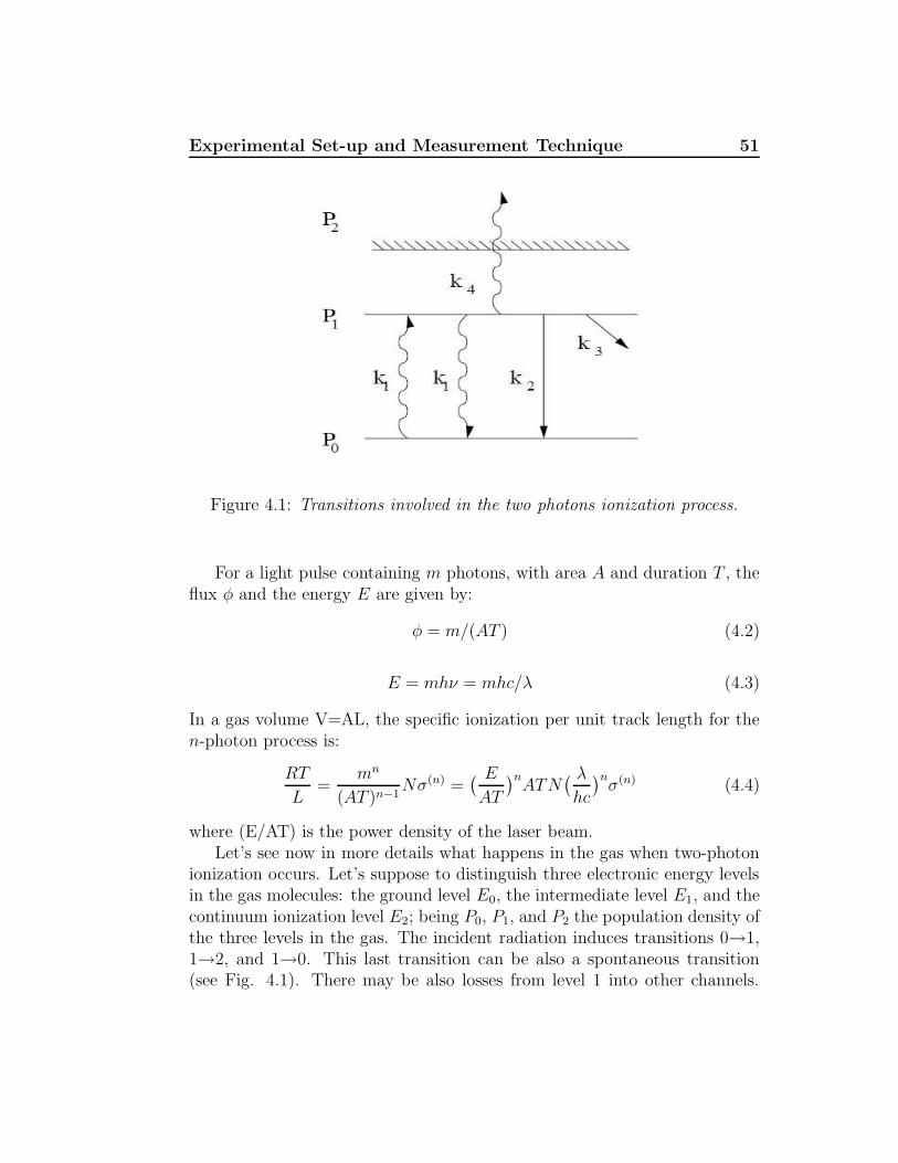
Experimental Set-up and Measurement Technique 51
Figure 4.1: Transitions involved in the two photons ionization process.
For a light pulse containing m photons, with area A and duration T , theflux φ and the energy E are given by:
φ = m/(AT ) (4.2)
E = mhν = mhc/λ (4.3)
In a gas volume V=AL, the specific ionization per unit track length for then-photon process is:
RT
L=
mn
(AT )n−1Nσ(n) =
( E
AT
)nATN
( λ
hc
)nσ(n) (4.4)
where (E/AT) is the power density of the laser beam.Let’s see now in more details what happens in the gas when two-photon
ionization occurs. Let’s suppose to distinguish three electronic energy levelsin the gas molecules: the ground level E0, the intermediate level E1, and thecontinuum ionization level E2; being P0, P1, and P2 the population density ofthe three levels in the gas. The incident radiation induces transitions 0→1,1→2, and 1→0. This last transition can be also a spontaneous transition(see Fig. 4.1). There may be also losses from level 1 into other channels.
Experimental Set-up and Measurement Technique 52
The transition rates per molecule are denoted by k1 (0→1,1→0 stimulated),k2 (1→0 spontaneously), k3 (1→ other channels), and k4 (1→2 ionization).They are determined by the incident flux and by the internal transitionmechanism.
The differential equations that rule the level populations can be writtenas follow (the primes denote time derivatives):
P′
0(t) = −k1P0(t) + (k1 + k2)P1(t) (4.5)
P′
1(t) = +k1P0(t) − (k1 + k2 + k3 + k4)P1(t) (4.6)
P′
2(t) = +k4P1(t) (4.7)
The rate per molecule k1 is taken to be proportional to the incoming fluxφ of photons through the cross-section σ01 for the process 0→1:
k1 = σ01φ (4.8)
The transition rate P′
2(t) give the rate of ionization. From Eq. 4.7, it resultsto be proportional to the density P1(t) of the intermediate state and to thecorresponding rate per molecules, k4 given by:
k4 = σ12φ (4.9)
The first two equation, 4.5and 4.6, are a system of homogeneous lineardifferential equation. In order to solve the system we have to do a variabletransformation that separates the equations. The eigenvalues s1 and s2 ofthe coefficient matrix are given by zeroing the determinant:
∣
∣
∣
∣
−k1 − s k1 + k2
k1 −(∑
k) − s
∣
∣
∣
∣
= 0 (4.10)
where∑
k = k1 + k2 + k3 + k4. Solving the equation we get:
s1,2 = −∑
k + k1
2±
[(
∑
k + k1
2
)2
− k1(k3 + k4)]1/2
(4.11)
These two eigenvalues are real and negative and we assume s2<s1<0. Atthis point we can find the solutions of the differential equations 4.7 applying
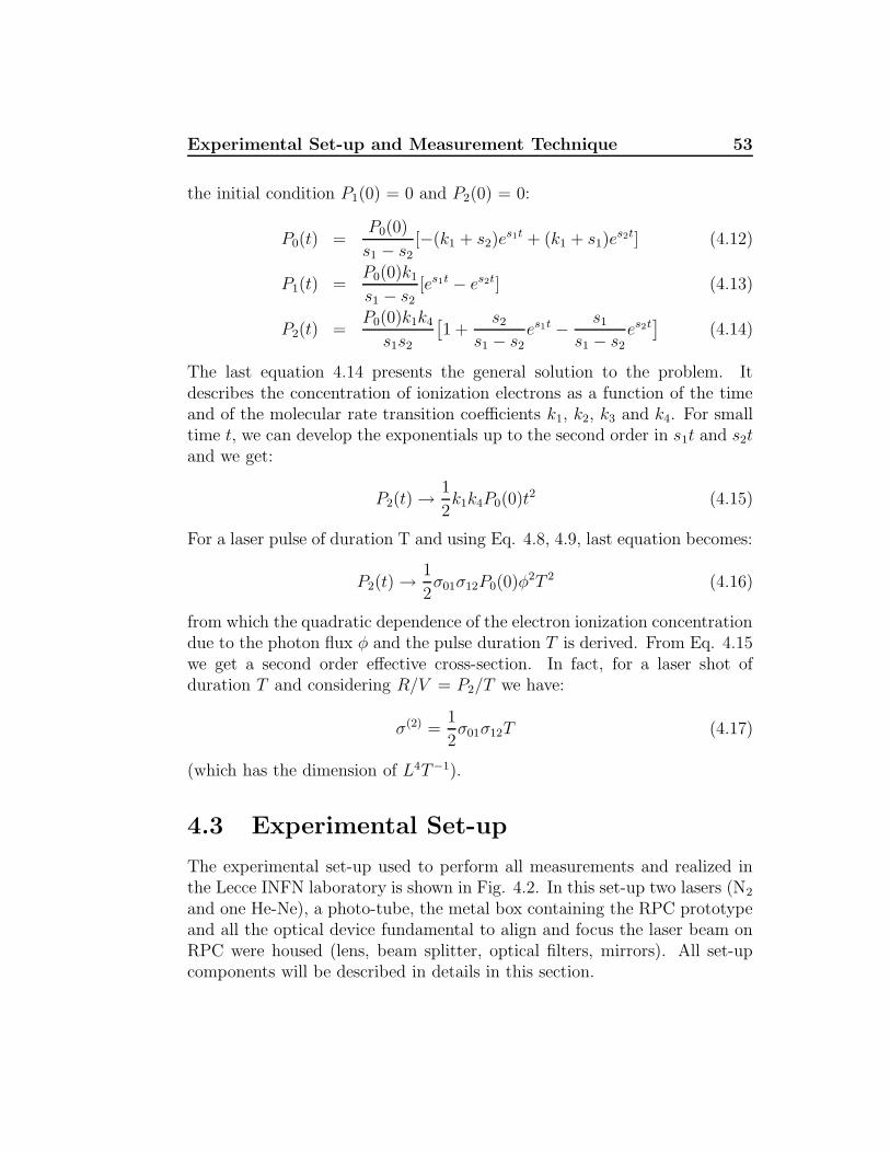
Experimental Set-up and Measurement Technique 53
the initial condition P1(0) = 0 and P2(0) = 0:
P0(t) =P0(0)
s1 − s2[−(k1 + s2)e
s1t + (k1 + s1)es2t] (4.12)
P1(t) =P0(0)k1
s1 − s2
[es1t − es2t] (4.13)
P2(t) =P0(0)k1k4
s1s2
[
1 +s2
s1 − s2es1t − s1
s1 − s2es2t
]
(4.14)
The last equation 4.14 presents the general solution to the problem. Itdescribes the concentration of ionization electrons as a function of the timeand of the molecular rate transition coefficients k1, k2, k3 and k4. For smalltime t, we can develop the exponentials up to the second order in s1t and s2tand we get:
P2(t) →1
2k1k4P0(0)t2 (4.15)
For a laser pulse of duration T and using Eq. 4.8, 4.9, last equation becomes:
P2(t) →1
2σ01σ12P0(0)φ2T 2 (4.16)
from which the quadratic dependence of the electron ionization concentrationdue to the photon flux φ and the pulse duration T is derived. From Eq. 4.15we get a second order effective cross-section. In fact, for a laser shot ofduration T and considering R/V = P2/T we have:
σ(2) =1
2σ01σ12T (4.17)
(which has the dimension of L4T−1).
4.3 Experimental Set-up
The experimental set-up used to perform all measurements and realized inthe Lecce INFN laboratory is shown in Fig. 4.2. In this set-up two lasers (N2
and one He-Ne), a photo-tube, the metal box containing the RPC prototypeand all the optical device fundamental to align and focus the laser beam onRPC were housed (lens, beam splitter, optical filters, mirrors). All set-upcomponents will be described in details in this section.
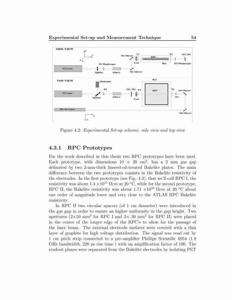
Experimental Set-up and Measurement Technique 54
x
y
z
x
y
N2 Laser
Splitter
D1 Diaphragm
Filters M1 Mirror
Lens Box
RPC
N2 Laser
Splitter Filters
Box
RPCD1
He−Ne Laser
D2
M3 Mirror
Phototube
M3, M4
SIDE VIEW
TOP VIEW
M2 Mirror T1 T2
Lens
M1, M2 T1 T2
D2 Diaphragm
M4 Mirror
Figure 4.2: Experimental Set-up scheme: side view and top view
4.3.1 RPC Prototypes
For the work described in this thesis two RPC prototypes have been used.Each prototype, with dimensions 10 × 20 cm2, has a 2 mm gas gapdelimited by two 2-mm-thick linseed-oil-treated Bakelite plates. The maindifference between the two prototypes consists in the Bakelite resistivity ofthe electrodes. In the first prototype (see Fig. 4.3), that we’ll call RPC I, theresistivity was about 1.4 ×10¹¹ Ωcm at 20 oC, while for the second prototype,RPC II, the Bakelite resistivity was about 1.71 ×10¹⁰ Ωcm at 20 oC aboutone order of magnitude lower and very close to the ATLAS RPC Bakeliteresistivity.
In RPC II two circular spacers (of 1 cm diameter) were introduced inthe gas gap in order to ensure an higher uniformity in the gap height. Twoapertures (2×50 mm2 for RPC I and 2× 30 mm2 for RPC II) were placedin the center of the longer edge of the RPC’s to allow for the passage ofthe laser beam. The external electrode surfaces were covered with a thinlayer of graphite for high voltage distribution. The signal was read out by1 cm pitch strip connected to a pre-amplifier Phillips Scientific 6954 (1.8GHz bandwidth, 220 ps rise time ) with an amplification factor of 100. Thereadout planes were separated from the Bakelite electrodes by isolating PET
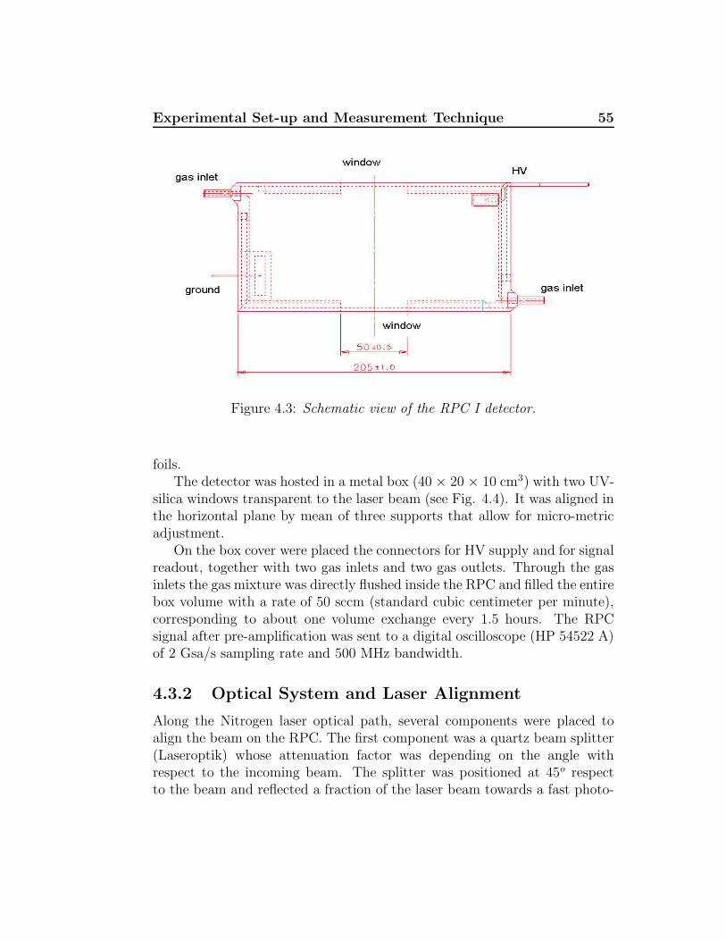
Experimental Set-up and Measurement Technique 55
Figure 4.3: Schematic view of the RPC I detector.
foils.The detector was hosted in a metal box (40 × 20 × 10 cm3) with two UV-
silica windows transparent to the laser beam (see Fig. 4.4). It was aligned inthe horizontal plane by mean of three supports that allow for micro-metricadjustment.
On the box cover were placed the connectors for HV supply and for signalreadout, together with two gas inlets and two gas outlets. Through the gasinlets the gas mixture was directly flushed inside the RPC and filled the entirebox volume with a rate of 50 sccm (standard cubic centimeter per minute),corresponding to about one volume exchange every 1.5 hours. The RPCsignal after pre-amplification was sent to a digital oscilloscope (HP 54522 A)of 2 Gsa/s sampling rate and 500 MHz bandwidth.
4.3.2 Optical System and Laser Alignment
Along the Nitrogen laser optical path, several components were placed toalign the beam on the RPC. The first component was a quartz beam splitter(Laseroptik) whose attenuation factor was depending on the angle withrespect to the incoming beam. The splitter was positioned at 45o respectto the beam and reflected a fraction of the laser beam towards a fast photo-
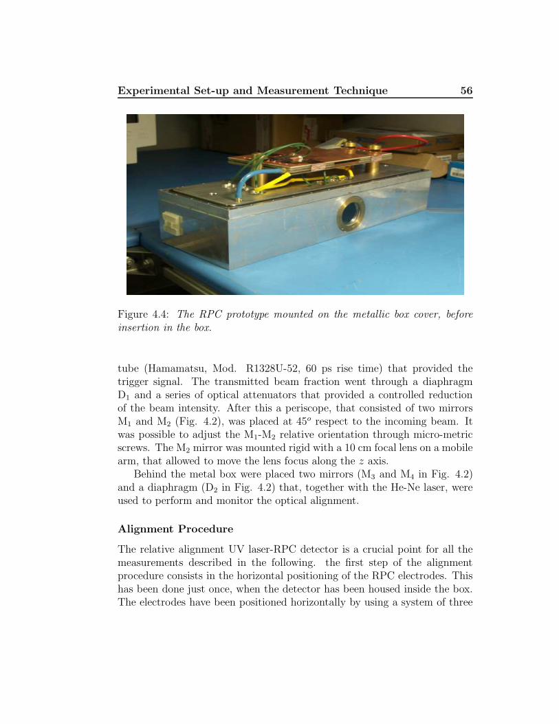
Experimental Set-up and Measurement Technique 56
Figure 4.4: The RPC prototype mounted on the metallic box cover, beforeinsertion in the box.
tube (Hamamatsu, Mod. R1328U-52, 60 ps rise time) that provided thetrigger signal. The transmitted beam fraction went through a diaphragmD1 and a series of optical attenuators that provided a controlled reductionof the beam intensity. After this a periscope, that consisted of two mirrorsM1 and M2 (Fig. 4.2), was placed at 45o respect to the incoming beam. Itwas possible to adjust the M1-M2 relative orientation through micro-metricscrews. The M2 mirror was mounted rigid with a 10 cm focal lens on a mobilearm, that allowed to move the lens focus along the z axis.
Behind the metal box were placed two mirrors (M3 and M4 in Fig. 4.2)and a diaphragm (D2 in Fig. 4.2) that, together with the He-Ne laser, wereused to perform and monitor the optical alignment.
Alignment Procedure
The relative alignment UV laser-RPC detector is a crucial point for all themeasurements described in the following. the first step of the alignmentprocedure consists in the horizontal positioning of the RPC electrodes. Thishas been done just once, when the detector has been housed inside the box.The electrodes have been positioned horizontally by using a system of three
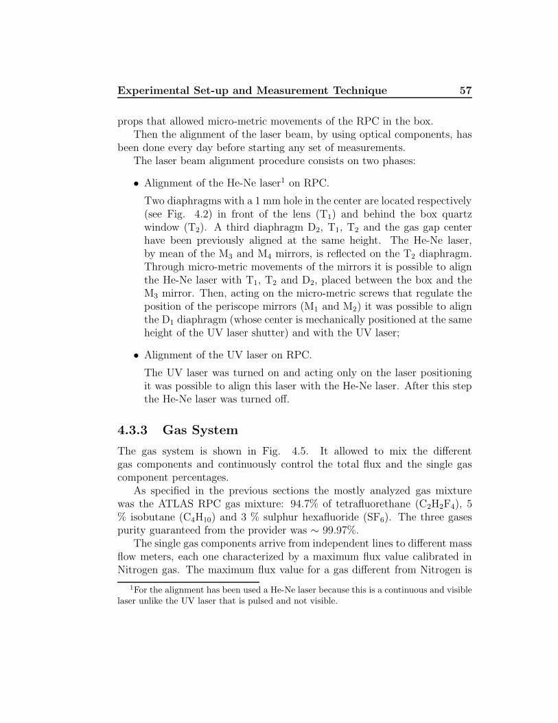
Experimental Set-up and Measurement Technique 57
props that allowed micro-metric movements of the RPC in the box.Then the alignment of the laser beam, by using optical components, has
been done every day before starting any set of measurements.The laser beam alignment procedure consists on two phases:
• Alignment of the He-Ne laser1 on RPC.
Two diaphragms with a 1 mm hole in the center are located respectively(see Fig. 4.2) in front of the lens (T1) and behind the box quartzwindow (T2). A third diaphragm D2, T1, T2 and the gas gap centerhave been previously aligned at the same height. The He-Ne laser,by mean of the M3 and M4 mirrors, is reflected on the T2 diaphragm.Through micro-metric movements of the mirrors it is possible to alignthe He-Ne laser with T1, T2 and D2, placed between the box and theM3 mirror. Then, acting on the micro-metric screws that regulate theposition of the periscope mirrors (M1 and M2) it was possible to alignthe D1 diaphragm (whose center is mechanically positioned at the sameheight of the UV laser shutter) and with the UV laser;
• Alignment of the UV laser on RPC.
The UV laser was turned on and acting only on the laser positioningit was possible to align this laser with the He-Ne laser. After this stepthe He-Ne laser was turned off.
4.3.3 Gas System
The gas system is shown in Fig. 4.5. It allowed to mix the differentgas components and continuously control the total flux and the single gascomponent percentages.
As specified in the previous sections the mostly analyzed gas mixturewas the ATLAS RPC gas mixture: 94.7% of tetrafluorethane (C2H2F4), 5% isobutane (C4H10) and 3 % sulphur hexafluoride (SF6). The three gasespurity guaranteed from the provider was ∼ 99.97%.
The single gas components arrive from independent lines to different massflow meters, each one characterized by a maximum flux value calibrated inNitrogen gas. The maximum flux value for a gas different from Nitrogen is
1For the alignment has been used a He-Ne laser because this is a continuous and visiblelaser unlike the UV laser that is pulsed and not visible.
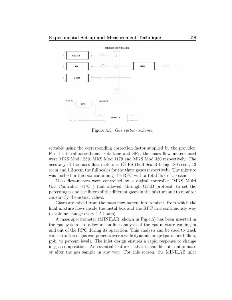
Experimental Set-up and Measurement Technique 58
RPC
MINILAB
GAS IN GAS OUT
C2H2F4
C4H10
SF6 MIXER
MKS GAS CONTROLLER
Figure 4.5: Gas system scheme.
settable using the corresponding correction factor supplied by the provider.For the tetrafluoroethane, isobutane and SF6, the mass flow meters usedwere MKS Mod 1259, MKS Mod 1179 and MKS Mod 330 respectively. Theaccuracy of the mass flow meters is 1% FS (Full Scale) being 180 sccm, 13sccm and 1.3 sccm the full scales for the three gases respectively. The mixturewas flushed in the box containing the RPC with a total flux of 50 sccm.
Mass flow-meters were controlled by a digital controller (MKS MultiGas Controller 647C ) that allowed, through GPIB protocol, to set thepercentages and the fluxes of the different gases in the mixture and to monitorconstantly the actual values.
Gases are mixed from the mass flow-meters into a mixer, from which thefinal mixture flows inside the metal box and the RPC in a continuously way(a volume change every 1.5 hours).
A mass spectrometer (MINILAB, shown in Fig.4.5) has been inserted inthe gas system. to allow an on-line analysis of the gas mixture coming inand out of the RPC during its operation. This analysis can be used to trackconcentration of gas components over a wide dynamic range (parts per billion,ppb, to percent level). The inlet design ensures a rapid response to changein gas composition. An essential feature is that it should not contaminateor alter the gas sample in any way. For this reason, the MINILAB inlet
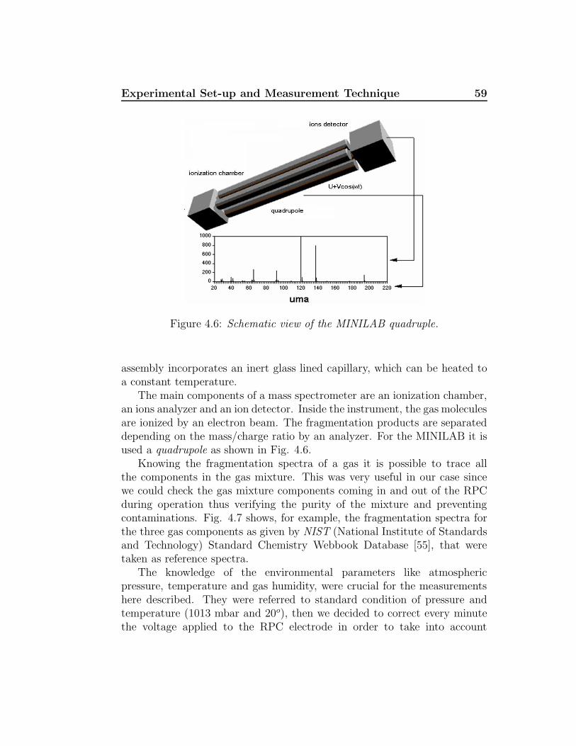
Experimental Set-up and Measurement Technique 59
Figure 4.6: Schematic view of the MINILAB quadruple.
assembly incorporates an inert glass lined capillary, which can be heated toa constant temperature.
The main components of a mass spectrometer are an ionization chamber,an ions analyzer and an ion detector. Inside the instrument, the gas moleculesare ionized by an electron beam. The fragmentation products are separateddepending on the mass/charge ratio by an analyzer. For the MINILAB it isused a quadrupole as shown in Fig. 4.6.
Knowing the fragmentation spectra of a gas it is possible to trace allthe components in the gas mixture. This was very useful in our case sincewe could check the gas mixture components coming in and out of the RPCduring operation thus verifying the purity of the mixture and preventingcontaminations. Fig. 4.7 shows, for example, the fragmentation spectra forthe three gas components as given by NIST (National Institute of Standardsand Technology) Standard Chemistry Webbook Database [55], that weretaken as reference spectra.
The knowledge of the environmental parameters like atmosphericpressure, temperature and gas humidity, were crucial for the measurementshere described. They were referred to standard condition of pressure andtemperature (1013 mbar and 20o), then we decided to correct every minutethe voltage applied to the RPC electrode in order to take into account
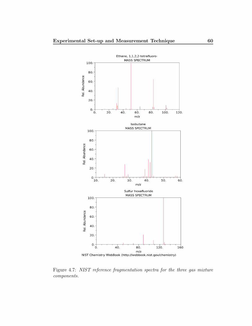
Experimental Set-up and Measurement Technique 60
Figure 4.7: NIST reference fragmentation spectra for the three gas mixturecomponents.
Experimental Set-up and Measurement Technique 61
any change of pressure and temperature. The voltage Vcorr really appliedwas obtained by the voltage value set (Vset) by the HV system and by themeasured values of pressure and temperature (Pmeas,Tmeas) as follows:
Vcorr = VsetPcorrTcorr (4.18)
Pcorr =Pmeas
1013(4.19)
Tcorr =293.15
Tmeas + 273.15(4.20)
Temperature and humidity were measured by two commercial probes.The probe measuring the temperature (Mod. IH-3602C) consists in a RTDsensitive to the temperature variations. Applying a constant current valueand reading back the voltage, a temperature value can be obtained by acalibration formula given by the provider. The temperature is readout insidethe experimental area. The humidity probe (HONEYWELL, MOd. HIH-4000-001) was inserted directly inside the metallic box and can thereforemeasure the gas mixture moisture. Also in this case we got back avoltage value from the probe which was converted in relative humidity bya calibration formula. The atmospheric pressure was measured by mean ofa transducer (MKS Baratron) with an accuracy of ∆P/P ∼ 10−4 mbar.
The two probes and the barometer were powered and read back by aVXI (Tektronix VX1410 Intelliframe), composed by a crate and severalmodules intercommunicating using a VXI protocol: a multichannel DACmodule (Digital to Analog Converter), Mod. AO-48XDC, supplied thevoltage and the current necessary to power the probes and the Baratron, anADC module (Analog to Digital Converter), Mod. MIO-64XE-10, performedthe measurements, finally a module VXI-MXI allowed the connection of thebus (that housed all the module) to the computer. The connection to thecomputer was realized through a serial interface MXI terminated with a PCIboard compatible with the computer.
4.3.4 High Voltage System
High voltage (HV) for the photo-tube and the RPC operations was suppliedthrough the system SY127 provided by CAEN [56]. The system is composedby one standard crate that houses a Control Unit and several HV plug-inchannel modules. It can be locally monitored and controlled via on-board
Experimental Set-up and Measurement Technique 62
alpha-numeric keypad and display. Remote control is also possible via RS-232-C port and it was the one used, by developing a dedicated softwarewritten in C++ language. Over-current and over-voltage protections whereimplemented in the software development phase together with channel tripdetection and switch-off control.
Two HV modules have been used: a 4 channels module Mod. A333,providing 4/3 kV voltage with positive polarity used to power the photo-tube and a 2 channels Mod. A329, providing 15 kV voltage with positivepolarity, used to apply HV to the RPC.
4.3.5 Micro-metric Movements System
Movements along the direction parallel to the laser beam (y in Fig. 4.2)and perpendicular to the beam (x) were performed through a very highprecision motorized bench VISIONCONTROL Mod. MC 841/1, ServiceMotor-control. It is composed of a marble bench on which two arms arepositioned; the one perpendicular to the beam direction is fixed to the benchand supports the second arm (in direction parallel to the beam). These twoarms were equipped with step motors and linear digital measuring rod. Thelinear precision of the axis, as provided by supplier, was δS = (3 + 2 ×L/1000) µm, where L is the distance in mm of the positioning point fromthe starting point.
The focal lens was mounted on a micro-metric motor that allowed tomove along the z direction the focus inside the gas gap with a precision of2µm/100mm. This motor is a Physic Instrument Mod. 415DG and allowsmovements up to 150 mm. It was remotely controlled by a Motor Controlboard Mod. C842.40 DC that can interface up to four different micro-metricmotors.
From the provider specification, the high voltage module riproducibilityis 1% of the set value at half full scale and 0.4% in all other ranges.
4.3.6 Nitrogen Laser
Ionization inside the RPC gas gap was induced by mean of the Nitrogen laserMod. MNL 200 LD from Lasertechnik (Berlin) that produces UV radiationwith λ = 337 nm. The main parameters characterizing the laser are reportedin table 4.1. The laser is controlled via RS232 port. The software that allows
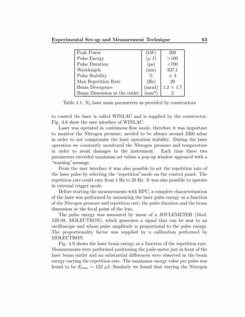
Experimental Set-up and Measurement Technique 63
Peak Power (kW) 200Pulse Energy (µ J) >100Pulse Duration (ps) <700Wavelength (nm) 337.1Pulse Stability % ± 3Max Repetition Rate (Hz) 20Beam Divergence (mrad) 1.2 × 1.7Beam Dimension at the outlet (mm2) 2
Table 4.1: N2 laser main parameters as provided by constructors
to control the laser is called WINLAC and is supplied by the constructor.Fig. 4.8 show the user interface of WINLAC.
Laser was operated in continuous flow mode, therefore it was importantto monitor the Nitrogen pressure, needed to be always around 2300 mbarin order to not compromise the laser operation stability. During the laseroperation we constantly monitored the Nitrogen pressure and temperaturein order to avoid damages to the instrument. Each time these twoparameters exceeded maximum set values a pop-up window appeared with a“warning”message.
From the user interface it was also possible to set the repetition rate ofthe laser pulse by selecting the “repetition”mode on the control panel. Therepetition rate could vary from 1 Hz to 20 Hz. It was also possible to operatein external trigger mode.
Before starting the measurements with RPC, a complete characterizationof the laser was performed by measuring the laser pulse energy as a functionof the Nitrogen pressure and repetition rate, the pulse duration and the beamdimension at the focal point of the lens.
The pulse energy was measured by mean of a JOULEMETER (Mod.J3S-09, MOLECTRON), which generates a signal that can be sent to anoscilloscope and whose pulse amplitude is proportional to the pulse energy.The proportionality factor was supplied by a calibration performed byMOLECTRON.
Fig. 4.9 shows the laser beam energy as a function of the repetition rate.Measurements were performed positioning the joule-meter just in front of thelaser beam outlet and no substantial differences were observed in the beamenergy varying the repetition rate. The maximum energy value per pulse wasfound to be Emax ∼ 122 µJ. Similarly we found that varying the Nitrogen
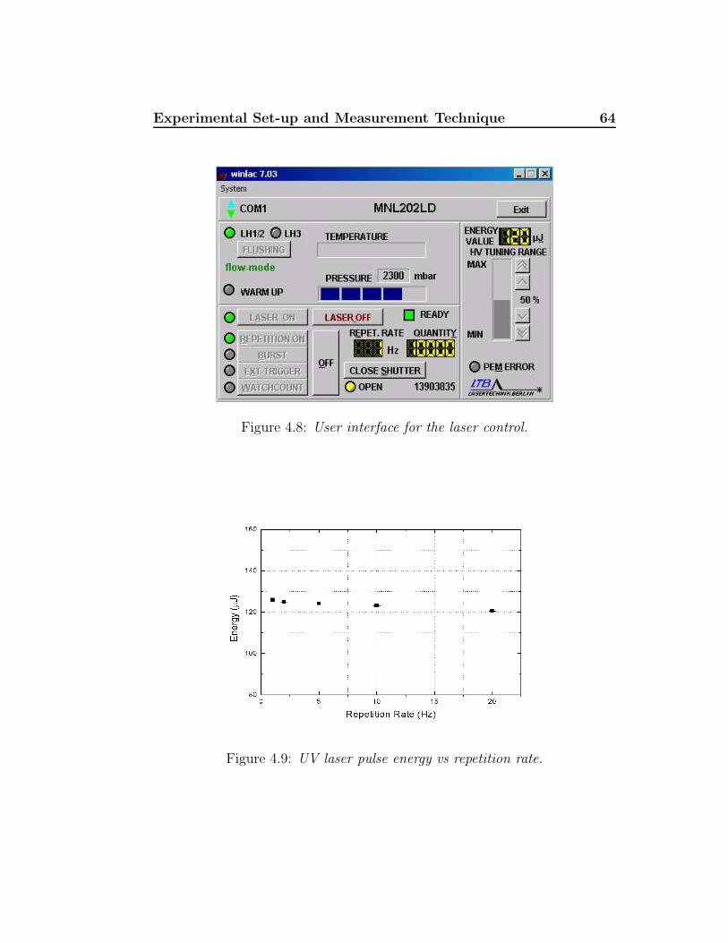
Experimental Set-up and Measurement Technique 64
Figure 4.8: User interface for the laser control.
Figure 4.9: UV laser pulse energy vs repetition rate.
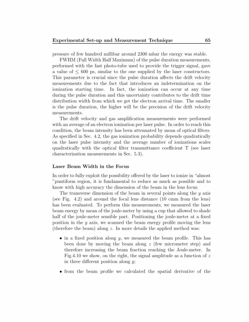
Experimental Set-up and Measurement Technique 65
pressure of few hundred millibar around 2300 mbar the energy was stable.FWHM (Full Width Half Maximum) of the pulse duration measurements,
performed with the fast photo-tube used to provide the trigger signal, gavea value of ≤ 600 ps, similar to the one supplied by the laser constructors.This parameter is crucial since the pulse duration affects the drift velocitymeasurements due to the fact that introduces an indetermination on theionization starting time. In fact, the ionization can occur at any timeduring the pulse duration and this uncertainty contributes to the drift timedistribution width from which we get the electron arrival time. The smalleris the pulse duration, the higher will be the precision of the drift velocitymeasurements.
The drift velocity and gas amplification measurements were performedwith an average of an electron ionization per laser pulse. In order to reach thiscondition, the beam intensity has been attenuated by mean of optical filters.As specified in Sec. 4.2, the gas ionization probability depends quadraticallyon the laser pulse intensity and the average number of ionizations scalesquadratically with the optical filter transmittance coefficient T (see lasercharacterization measurements in Sec. 5.3).
Laser Beam Width in the Focus
In order to fully exploit the possibility offered by the laser to ionize in “almost”puntiform region, it is fundamental to reduce as much as possible and toknow with high accuracy the dimension of the beam in the lens focus.
The transverse dimension of the beam in several points along the y axis(see Fig. 4.2) and around the focal lens distance (10 cmm from the lens)has been evaluated. To perform this measurements, we measured the laserbeam energy by mean of the joule-meter by using a cup that allowed to shadehalf of the joule-meter sensible part. Positioning the joule-meter at a fixedposition in the y axis, we scanned the beam energy profile moving the lens(therefore the beam) along z. In more details the applied method was:
• in a fixed position along y, we measured the beam profile. This hasbeen done by moving the beam along z (few micrometer step) andtherefore increasing the beam fraction reaching the Joule-meter. InFig.4.10 we show, on the right, the signal amplitude as a function of zin three different position along y;
• from the beam profile we calculated the spatial derivative of the
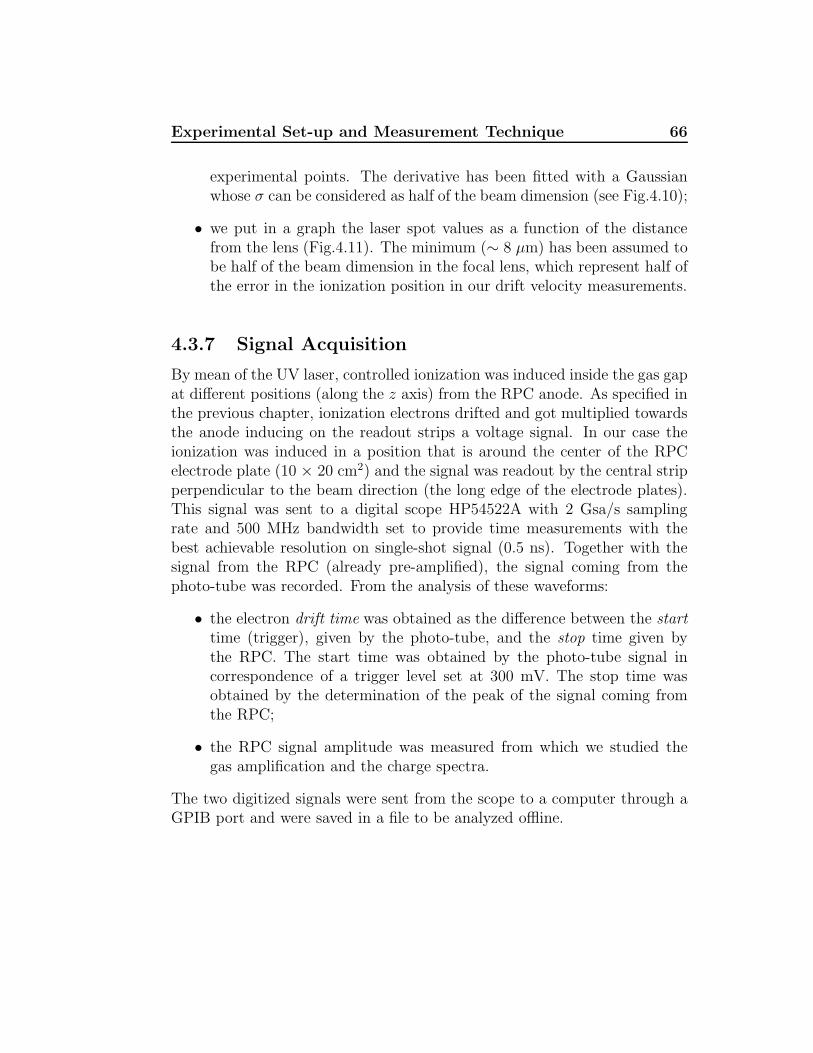
Experimental Set-up and Measurement Technique 66
experimental points. The derivative has been fitted with a Gaussianwhose σ can be considered as half of the beam dimension (see Fig.4.10);
• we put in a graph the laser spot values as a function of the distancefrom the lens (Fig.4.11). The minimum (∼ 8 µm) has been assumed tobe half of the beam dimension in the focal lens, which represent half ofthe error in the ionization position in our drift velocity measurements.
4.3.7 Signal Acquisition
By mean of the UV laser, controlled ionization was induced inside the gas gapat different positions (along the z axis) from the RPC anode. As specified inthe previous chapter, ionization electrons drifted and got multiplied towardsthe anode inducing on the readout strips a voltage signal. In our case theionization was induced in a position that is around the center of the RPCelectrode plate (10 × 20 cm2) and the signal was readout by the central stripperpendicular to the beam direction (the long edge of the electrode plates).This signal was sent to a digital scope HP54522A with 2 Gsa/s samplingrate and 500 MHz bandwidth set to provide time measurements with thebest achievable resolution on single-shot signal (0.5 ns). Together with thesignal from the RPC (already pre-amplified), the signal coming from thephoto-tube was recorded. From the analysis of these waveforms:
• the electron drift time was obtained as the difference between the starttime (trigger), given by the photo-tube, and the stop time given bythe RPC. The start time was obtained by the photo-tube signal incorrespondence of a trigger level set at 300 mV. The stop time wasobtained by the determination of the peak of the signal coming fromthe RPC;
• the RPC signal amplitude was measured from which we studied thegas amplification and the charge spectra.
The two digitized signals were sent from the scope to a computer through aGPIB port and were saved in a file to be analyzed offline.
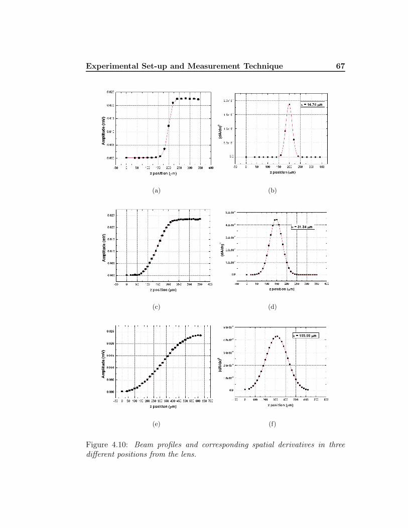
Experimental Set-up and Measurement Technique 67
(a) (b)
(c) (d)
(e) (f)
Figure 4.10: Beam profiles and corresponding spatial derivatives in threedifferent positions from the lens.
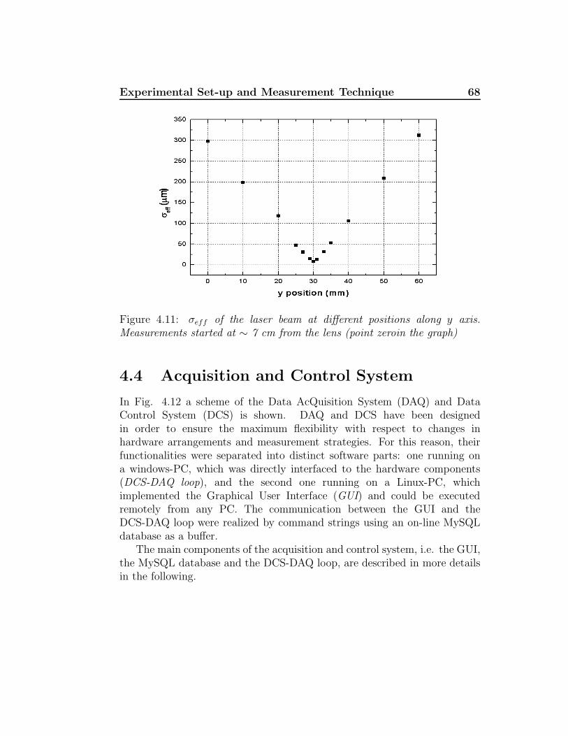
Experimental Set-up and Measurement Technique 68
Figure 4.11: σeff of the laser beam at different positions along y axis.Measurements started at ∼ 7 cm from the lens (point zeroin the graph)
4.4 Acquisition and Control System
In Fig. 4.12 a scheme of the Data AcQuisition System (DAQ) and DataControl System (DCS) is shown. DAQ and DCS have been designedin order to ensure the maximum flexibility with respect to changes inhardware arrangements and measurement strategies. For this reason, theirfunctionalities were separated into distinct software parts: one running ona windows-PC, which was directly interfaced to the hardware components(DCS-DAQ loop), and the second one running on a Linux-PC, whichimplemented the Graphical User Interface (GUI) and could be executedremotely from any PC. The communication between the GUI and theDCS-DAQ loop were realized by command strings using an on-line MySQLdatabase as a buffer.
The main components of the acquisition and control system, i.e. the GUI,the MySQL database and the DCS-DAQ loop, are described in more detailsin the following.
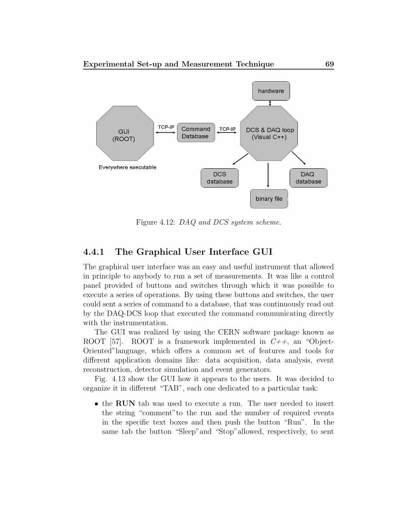
Experimental Set-up and Measurement Technique 69
Figure 4.12: DAQ and DCS system scheme.
4.4.1 The Graphical User Interface GUI
The graphical user interface was an easy and useful instrument that allowedin principle to anybody to run a set of measurements. It was like a controlpanel provided of buttons and switches through which it was possible toexecute a series of operations. By using these buttons and switches, the usercould sent a series of command to a database, that was continuously read outby the DAQ-DCS loop that executed the command communicating directlywith the instrumentation.
The GUI was realized by using the CERN software package known asROOT [57]. ROOT is a framework implemented in C++, an “Object-Oriented”language, which offers a common set of features and tools fordifferent application domains like: data acquisition, data analysis, eventreconstruction, detector simulation and event generators.
Fig. 4.13 show the GUI how it appears to the users. It was decided toorganize it in different “TAB”, each one dedicated to a particular task:
• the RUN tab was used to execute a run. The user needed to insertthe string “comment”to the run and the number of required eventsin the specific text boxes and then push the button “Run”. In thesame tab the button “Sleep”and “Stop”allowed, respectively, to sent
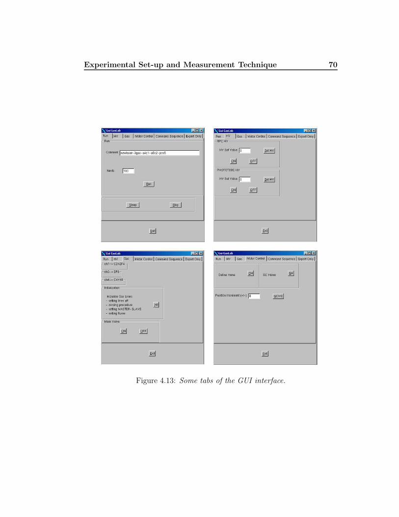
Experimental Set-up and Measurement Technique 70
Figure 4.13: Some tabs of the GUI interface.
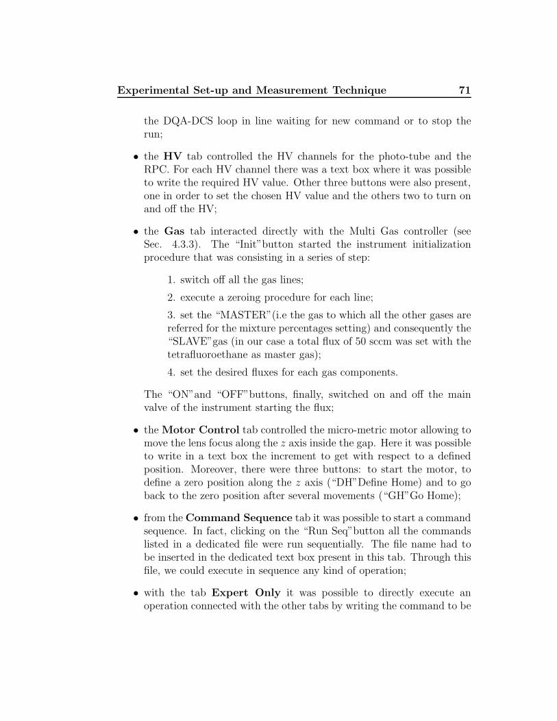
Experimental Set-up and Measurement Technique 71
the DQA-DCS loop in line waiting for new command or to stop therun;
• the HV tab controlled the HV channels for the photo-tube and theRPC. For each HV channel there was a text box where it was possibleto write the required HV value. Other three buttons were also present,one in order to set the chosen HV value and the others two to turn onand off the HV;
• the Gas tab interacted directly with the Multi Gas controller (seeSec. 4.3.3). The “Init”button started the instrument initializationprocedure that was consisting in a series of step:
1. switch off all the gas lines;
2. execute a zeroing procedure for each line;
3. set the “MASTER”(i.e the gas to which all the other gases arereferred for the mixture percentages setting) and consequently the“SLAVE”gas (in our case a total flux of 50 sccm was set with thetetrafluoroethane as master gas);
4. set the desired fluxes for each gas components.
The “ON”and “OFF”buttons, finally, switched on and off the mainvalve of the instrument starting the flux;
• the Motor Control tab controlled the micro-metric motor allowing tomove the lens focus along the z axis inside the gap. Here it was possibleto write in a text box the increment to get with respect to a definedposition. Moreover, there were three buttons: to start the motor, todefine a zero position along the z axis (“DH”Define Home) and to goback to the zero position after several movements (“GH”Go Home);
• from the Command Sequence tab it was possible to start a commandsequence. In fact, clicking on the “Run Seq”button all the commandslisted in a dedicated file were run sequentially. The file name had tobe inserted in the dedicated text box present in this tab. Through thisfile, we could execute in sequence any kind of operation;
• with the tab Expert Only it was possible to directly execute anoperation connected with the other tabs by writing the command to be
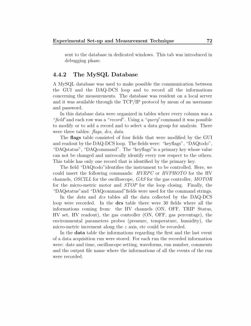
Experimental Set-up and Measurement Technique 72
sent to the database in dedicated windows. This tab was introduced indebugging phase.
4.4.2 The MySQL Database
A MySQL database was used to make possible the communication betweenthe GUI and the DAQ-DCS loop and to record all the informationsconcerning the measurements. The database was resident on a local serverand it was available through the TCP/IP protocol by mean of an usernameand password.
In this database data were organized in tables where every column was a“field”and each row was a “record”. Using a “query”command it was possibleto modify or to add a record and to select a data group for analysis. Therewere three tables: flags, dcs, data.
The flags table consisted of four fields that were modified by the GUIand readout by the DAQ-DCS loop. The fields were: “keyflags”, “DAQtodo”,“DAQstatus”, “DAQcommand”. The “keyflags”is a primary key whose valuecan not be changed and univocally identify every row respect to the others.This table has only one record that is identified by the primary key.
The field “DAQtodo”identifies the instrument to be controlled. Here, wecould insert the following commands: HVRPC or HVPHOTO for the HVchannels, OSCILL for the oscilloscope, GAS for the gas controller, MOTORfor the micro-metric motor and STOP for the loop closing. Finally, the“DAQstatus”and “DAQcommand”fields were used for the command strings.
In the data and dcs tables all the data collected by the DAQ-DCSloop were recorded. In the dcs table there were 30 fields where all theinformations coming from: the HV channels (ON, OFF, TRIP Status,HV set, HV readout), the gas controller (ON, OFF, gas percentage), theenvironmental parameters probes (pressure, temperature, humidity), themicro-metric increment along the z axis, etc could be recorded.
In the data table the informations regarding the first and the last eventof a data acquisition run were stored. For each run the recorded informationwere: date and time, oscilloscope setting, waveforms, run number, commentsand the output file name where the informations of all the events of the runwere recorded.
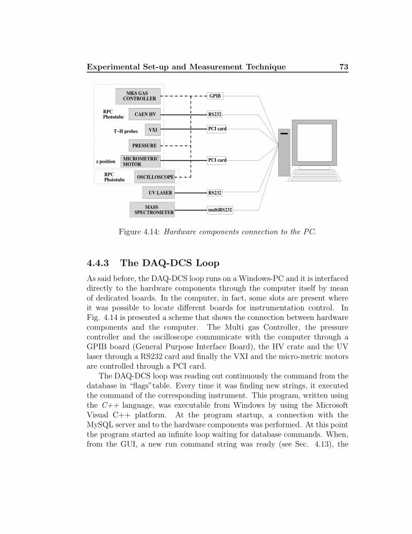
Experimental Set-up and Measurement Technique 73
MKS GASCONTROLLER
CAEN HV
VXI
PRESSURE
MICROMETRICMOTOR
OSCILLOSCOPE
UV LASER
SPECTROMETERMASS
GPIB
RS232
PCI card
PCI card
multiRS232
RS232
PhototubeRPC
PhototubeRPC
z position
T−H probes
Figure 4.14: Hardware components connection to the PC.
4.4.3 The DAQ-DCS Loop
As said before, the DAQ-DCS loop runs on a Windows-PC and it is interfaceddirectly to the hardware components through the computer itself by meanof dedicated boards. In the computer, in fact, some slots are present whereit was possible to locate different boards for instrumentation control. InFig. 4.14 is presented a scheme that shows the connection between hardwarecomponents and the computer. The Multi gas Controller, the pressurecontroller and the oscilloscope communicate with the computer through aGPIB board (General Purpose Interface Board), the HV crate and the UVlaser through a RS232 card and finally the VXI and the micro-metric motorsare controlled through a PCI card.
The DAQ-DCS loop was reading out continuously the command from thedatabase in “flags”table. Every time it was finding new strings, it executedthe command of the corresponding instrument. This program, written usingthe C++ language, was executable from Windows by using the MicrosoftVisual C++ platform. At the program startup, a connection with theMySQL server and to the hardware components was performed. At this pointthe program started an infinite loop waiting for database commands. When,from the GUI, a new run command string was ready (see Sec. 4.13), the
Experimental Set-up and Measurement Technique 74
DAQ-DCS loop read it and saved the oscilloscope waveforms in a file. In thisdata file, event by event, all the informations needed for the correct decodingof the signals were recorded. This was done in order to allow for an easyoff-line data analysis. The file was consisting of several blocks. An HaederRun described the run itself and held the oscilloscope preamble containingall the setting parameters needed to correctly decode the waveforms in theoff-line analysis. This was followed by the event-blocks. Each event consistedof an Haeder Event with the oscilloscope channels information and an HaederChannel followed by the signal sampling vector. As specified in the previoussections, the informations from the first and the last event were also savedin the “data”table of the database.
During the data acquisition, the DAQ-DCS loop saved in the“dcs”database table all the useful informations coming from theinstrumentation. This procedure was performed each minute to take intoaccount the pressure and temperature variations in order to adjust the HVapplied to the RPC electrodes.
4.4.4 The Off-line Software Analysis
The DAQ-DCS loop produces a binary file that is saved for the off-lineanalysis. In order to study the parameters of the gas mixture, we needed toderive the drift time and the RPC signal amplitude. This was done by usinga custom software written in C++ and using the ROOT package consistingof two distinct parts: signal decoding and waveforms analysis.
The first part decoded the waveforms of the binary files acquired duringthe run and recorded the informations in histograms that can be read out bya ROOT macro. Using this macro, it was possible, after performing a Fourieranalysis of the signals, to remove a noise correlated with the pulse laser thatwe could not shield, to obtain the drift time and the signal amplitude for eachionization event in the RPC. The filter was applied by using the DiscreteFourier Transform (DFT) through the Fast Fourier Transform (FFT). Formthe FFT frequencies spectrum, only frequencies lower that a chosen cutoffwere selected. At this point the inverse Fourier transformation (IFFT)was applied. The filter cutoff value was 280 MHz and it was chosen aftera dedicated preliminary analysis in order to not to introduce any signaldistortion.
Chapter 5
Experimental Results
5.1 Introduction
In this chapter we describe the measurements of the basic ATLAS RPCgas mixture parameters, such as electron drift velocity and gas amplificationand we analyze and discuss charge spectra. The gas mixture consists of94.7%C2H2F4+5%C4H10+0.3%SF6 and it was studied for the first time bydirect measurements using the localized laser spot as ionization source.
The experimental results reported in this section have been obtained withthe RPC II prototype. In a dedicated section measurements performed onRPC I prototype are shown and compared with results from RPC II.
As already mentioned in Sec. 4.3.3 all measurements refer to high voltagecorrected, in real time, for the environmental temperature T and pressure Pchanges.
5.2 Electron Avalanche Signal
As discussed in chapter 3, the induced current i(t) on the RPC readout stripis the charge image of the avalanche charge q(t) which grows in the gas anddrifts towards the anode. The two quantities are related by the formulas 3.19and 3.20, discussed in chapter 3:
i(t) = kvD
gq(t) (5.1)
where k is the “k-factor”, g = 2 mm is the gas gap thickness, vD is theelectron drift velocity and q(t) is the total avalanche charge at time t.
Experimental Results 76
We consider negligible the longitudinal avalanche spread, due to theelectron diffusion, and the contribution to the induced current of the positiveand negative ions drift. In this approximation the current should abruptlyterminate when the avalanche reaches the anode. Consequently, from thecurrent maximum is possible to estimate the total avalanche charge q(tD)and the drift time tD:
q(tD) =gipeak(tD)
kvD(5.2)
It’s possible, considering the amplifier gain G and its termination R, tocalibrate the peak voltage vpeak = v(tD), measured by recording the signalwaveform, in term of the total avalanche charge q(tD):
q(tD) =g
kvD
vpeak
GR≈ 5.52
[
pC
V
]
vpeak ≈ 3.4 × 10⁷
[
e−
V
]
vpeak (5.3)
where we have assumed vD = 145 µm/ns according to the drift velocityresults presented in Sec. 5.4. The electronic noise at the output of theamplifier was about 10 mV which corresponds to about 0.05 pC (= 3.4 ×10⁵ e−) equivalent noise charge, at least two order of magnitude below theRaether limit of about 108 e− and well below the saturated avalanche chargeof about 107 e−, characteristic of signal in our operating regime.
Fig. 5.1 shows a typical signal waveform corresponding to an avalancheinitiated by a laser pulse in single ionization condition reached by finelyreduce the beam intensity as described in Sec. 4.3.6. It is possible tonotice how the signal follows, approximately, a simple exponential law in therising part. The electric signal doesn’t change abruptly after the maximumis reached. This can be due to several factors as for example, to thetransfer function of the readout system, which is a complicated interplaybetween different parts: the graphite layer, the metal strips and the amplifier.Actually, an exhaustive and detailed explanation of the waveform featuresinvolves complex phenomena, but these phenomena have a modest impacton the extraction of the electron transport properties.
5.3 Laser Ionization Source Set-up
Fig. 5.2 shows the geometrical configuration of the RPC irradiated with thelaser light. The laser beam light was focused inside the 2 mm height gas gap
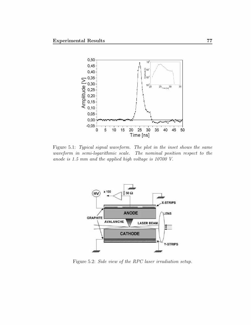
Experimental Results 77
Figure 5.1: Typical signal waveform. The plot in the inset shows the samewaveform in semi-logarithmic scale. The nominal position respect to theanode is 1.5 mm and the applied high voltage is 10700 V.
Figure 5.2: Side view of the RPC laser irradiation setup.
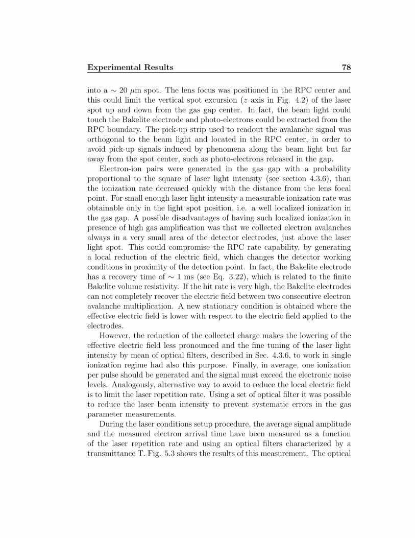
Experimental Results 78
into a ∼ 20 µm spot. The lens focus was positioned in the RPC center andthis could limit the vertical spot excursion (z axis in Fig. 4.2) of the laserspot up and down from the gas gap center. In fact, the beam light couldtouch the Bakelite electrode and photo-electrons could be extracted from theRPC boundary. The pick-up strip used to readout the avalanche signal wasorthogonal to the beam light and located in the RPC center, in order toavoid pick-up signals induced by phenomena along the beam light but faraway from the spot center, such as photo-electrons released in the gap.
Electron-ion pairs were generated in the gas gap with a probabilityproportional to the square of laser light intensity (see section 4.3.6), thanthe ionization rate decreased quickly with the distance from the lens focalpoint. For small enough laser light intensity a measurable ionization rate wasobtainable only in the light spot position, i.e. a well localized ionization inthe gas gap. A possible disadvantages of having such localized ionization inpresence of high gas amplification was that we collected electron avalanchesalways in a very small area of the detector electrodes, just above the laserlight spot. This could compromise the RPC rate capability, by generatinga local reduction of the electric field, which changes the detector workingconditions in proximity of the detection point. In fact, the Bakelite electrodehas a recovery time of ∼ 1 ms (see Eq. 3.22), which is related to the finiteBakelite volume resistivity. If the hit rate is very high, the Bakelite electrodescan not completely recover the electric field between two consecutive electronavalanche multiplication. A new stationary condition is obtained where theeffective electric field is lower with respect to the electric field applied to theelectrodes.
However, the reduction of the collected charge makes the lowering of theeffective electric field less pronounced and the fine tuning of the laser lightintensity by mean of optical filters, described in Sec. 4.3.6, to work in singleionization regime had also this purpose. Finally, in average, one ionizationper pulse should be generated and the signal must exceed the electronic noiselevels. Analogously, alternative way to avoid to reduce the local electric fieldis to limit the laser repetition rate. Using a set of optical filter it was possibleto reduce the laser beam intensity to prevent systematic errors in the gasparameter measurements.
During the laser conditions setup procedure, the average signal amplitudeand the measured electron arrival time have been measured as a functionof the laser repetition rate and using an optical filters characterized by atransmittance T. Fig. 5.3 shows the results of this measurement. The optical
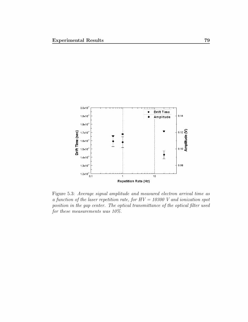
Experimental Results 79
Figure 5.3: Average signal amplitude and measured electron arrival time asa function of the laser repetition rate, for HV = 10300 V and ionization spotposition in the gap center. The optical transmittance of the optical filter usedfor these measurements was 10%.
Experimental Results 80
Figure 5.4: RPC mean pulse height (upper plot) and RPC counts fraction(lower plot) versus applied high voltage for two different optical filters withoptical transmittance T. Superimposed are the fits obtained by the logisticcumulative function described in Sec. 5.6.1. Data are taken with ionizationspot located at 1500 µm from the anode.
filter used in this case had a 10% optical transmittance and the position inthe gap was the same for all the measurements. Increasing the repetitionrate we observed a decrease of the signal amplitude and an increase of themeasured arrival time. This can be easily explained assuming that the localeffective electric field gradually decreased with increasing laser repetition ratethus producing a lower gas gain and larger drift time of the electrons to theanode.
Fig. 5.4 shows (lower plot) the fraction of events where an avalanchewas detected using a 10% and a 3.5% trasmittance optical filter, for differentvalues of the applied high voltage. For both optical filters is possible tonotice a plateau in the counting fraction for large enough high voltage values.The plateau counting fraction was interpreted as the product of the RPC
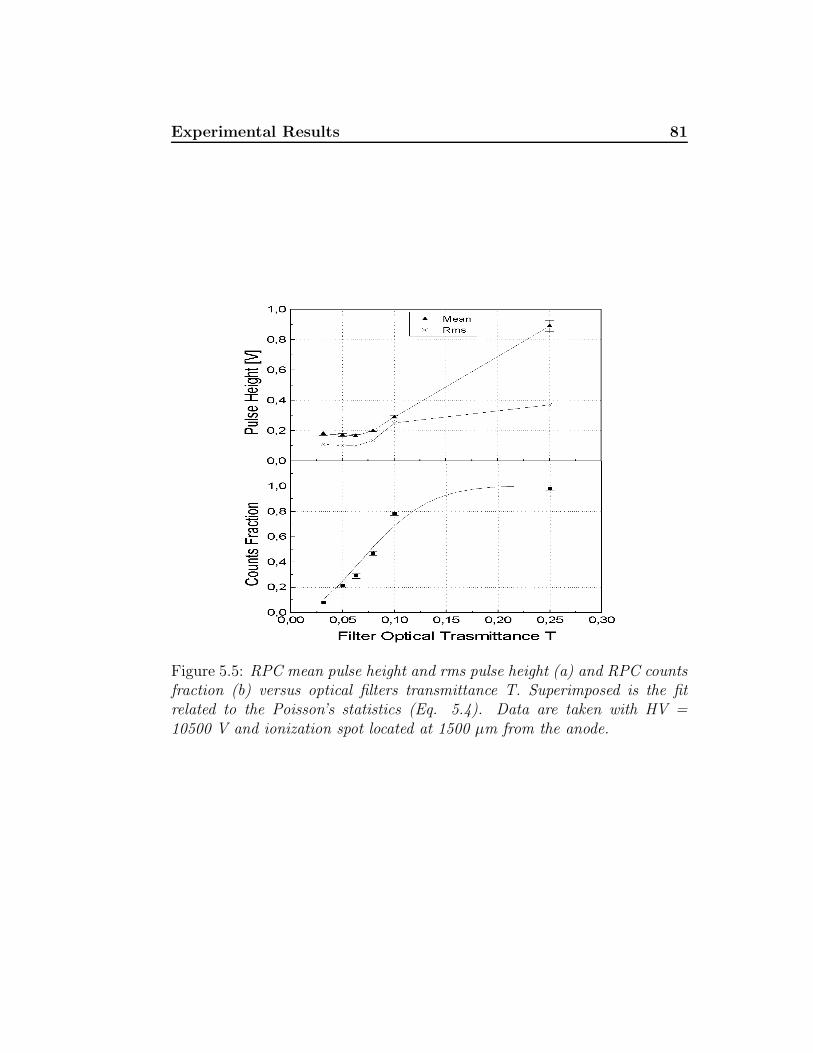
Experimental Results 81
Figure 5.5: RPC mean pulse height and rms pulse height (a) and RPC countsfraction (b) versus optical filters transmittance T. Superimposed is the fitrelated to the Poisson’s statistics (Eq. 5.4). Data are taken with HV =10500 V and ionization spot located at 1500 µm from the anode.
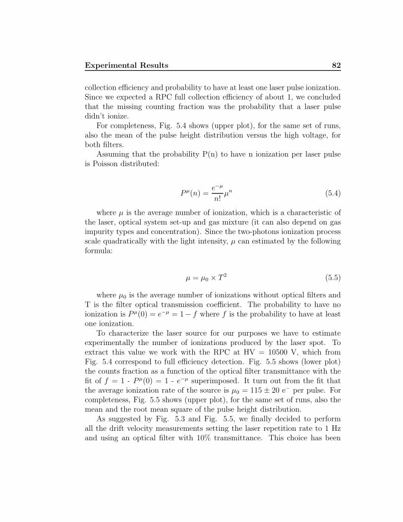
Experimental Results 82
collection efficiency and probability to have at least one laser pulse ionization.Since we expected a RPC full collection efficiency of about 1, we concludedthat the missing counting fraction was the probability that a laser pulsedidn’t ionize.
For completeness, Fig. 5.4 shows (upper plot), for the same set of runs,also the mean of the pulse height distribution versus the high voltage, forboth filters.
Assuming that the probability P(n) to have n ionization per laser pulseis Poisson distributed:
P µ(n) =e−µ
n!µn (5.4)
where µ is the average number of ionization, which is a characteristic ofthe laser, optical system set-up and gas mixture (it can also depend on gasimpurity types and concentration). Since the two-photons ionization processscale quadratically with the light intensity, µ can estimated by the followingformula:
µ = µ0 × T 2 (5.5)
where µ0 is the average number of ionizations without optical filters andT is the filter optical transmission coefficient. The probability to have noionization is P µ(0) = e−µ = 1− f where f is the probability to have at leastone ionization.
To characterize the laser source for our purposes we have to estimateexperimentally the number of ionizations produced by the laser spot. Toextract this value we work with the RPC at HV = 10500 V, which fromFig. 5.4 correspond to full efficiency detection. Fig. 5.5 shows (lower plot)the counts fraction as a function of the optical filter transmittance with thefit of f = 1 - P µ(0) = 1 - e−µ superimposed. It turn out from the fit thatthe average ionization rate of the source is µ0 = 115 ± 20 e− per pulse. Forcompleteness, Fig. 5.5 shows (upper plot), for the same set of runs, also themean and the root mean square of the pulse height distribution.
As suggested by Fig. 5.3 and Fig. 5.5, we finally decided to performall the drift velocity measurements setting the laser repetition rate to 1 Hzand using an optical filter with 10% transmittance. This choice has been
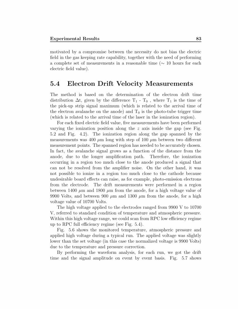
Experimental Results 83
motivated by a compromise between the necessity do not bias the electricfield in the gas keeping rate capability, together with the need of performinga complete set of measurements in a reasonable time (∼ 10 hours for eachelectric field value).
5.4 Electron Drift Velocity Measurements
The method is based on the determination of the electron drift timedistribution ∆t, given by the difference T1 - T0 , where T1 is the time ofthe pick-up strip signal maximum (which is related to the arrival time ofthe electron avalanche on the anode) and T0 is the photo-tube trigger time(which is related to the arrival time of the laser in the ionization region).
For each fixed electric field value, five measurements have been performedvarying the ionization position along the z axis inside the gap (see Fig.5.2 and Fig. 4.2). The ionization region along the gap spanned by themeasurements was 400 µm long with step of 100 µm between two differentmeasurement points. The spanned region has needed to be accurately chosen.In fact, the avalanche signal grows as a function of the distance from theanode, due to the longer amplification path. Therefore, the ionizationoccurring in a region too much close to the anode produced a signal thatcan not be resolved from the amplifier noise. On the other hand, it wasnot possible to ionize in a region too much close to the cathode becauseundesirable board effects can raise, as for example, photo-emission electronsfrom the electrode. The drift measurements were performed in a regionbetween 1400 µm and 1800 µm from the anode, for a high voltage value of9900 Volts, and between 900 µm and 1300 µm from the anode, for a highvoltage value of 10700 Volts.
The high voltage applied to the electrodes ranged from 9900 V to 10700V, referred to standard condition of temperature and atmospheric pressure.Within this high voltage range, we could scan from RPC low efficiency regimeup to RPC full efficiency regime (see Fig. 5.4).
Fig. 5.6 shows the monitored temperature, atmospheric pressure andapplied high voltage during a typical run. The applied voltage was slightlylower than the set voltage (in this case the normalized voltage is 9900 Volts)due to the temperature and pressure correction.
By performing the waveform analysis, for each run, we got the drifttime and the signal amplitude on event by event basis. Fig. 5.7 shows
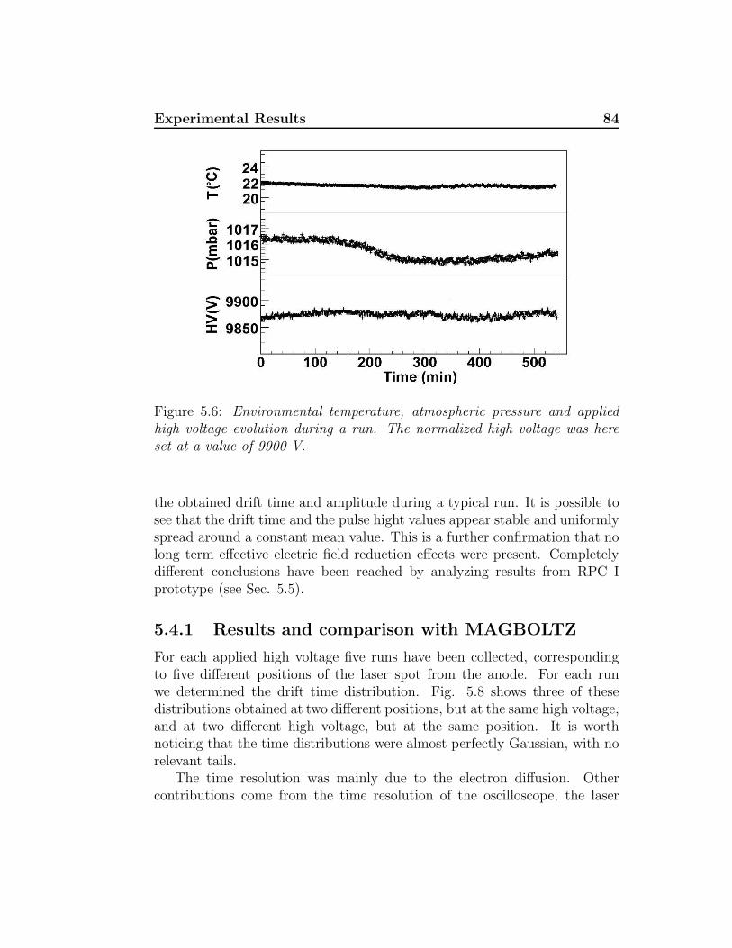
Experimental Results 84
Figure 5.6: Environmental temperature, atmospheric pressure and appliedhigh voltage evolution during a run. The normalized high voltage was hereset at a value of 9900 V.
the obtained drift time and amplitude during a typical run. It is possible tosee that the drift time and the pulse hight values appear stable and uniformlyspread around a constant mean value. This is a further confirmation that nolong term effective electric field reduction effects were present. Completelydifferent conclusions have been reached by analyzing results from RPC Iprototype (see Sec. 5.5).
5.4.1 Results and comparison with MAGBOLTZ
For each applied high voltage five runs have been collected, correspondingto five different positions of the laser spot from the anode. For each runwe determined the drift time distribution. Fig. 5.8 shows three of thesedistributions obtained at two different positions, but at the same high voltage,and at two different high voltage, but at the same position. It is worthnoticing that the time distributions were almost perfectly Gaussian, with norelevant tails.
The time resolution was mainly due to the electron diffusion. Othercontributions come from the time resolution of the oscilloscope, the laser
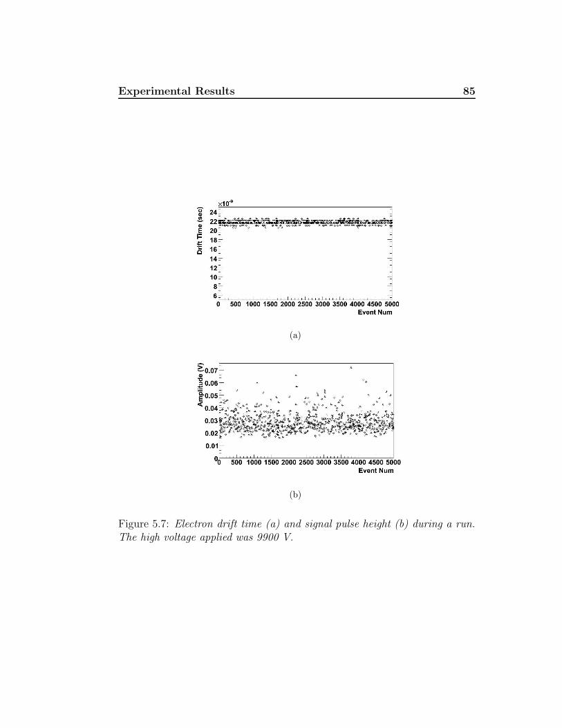
Experimental Results 85
(a)
(b)
Figure 5.7: Electron drift time (a) and signal pulse height (b) during a run.The high voltage applied was 9900 V.
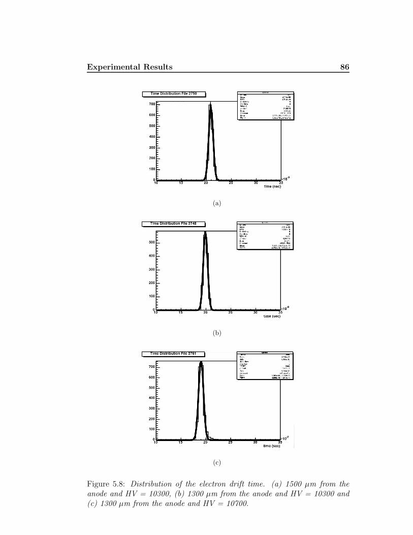
Experimental Results 86
(a)
(b)
(c)
Figure 5.8: Distribution of the electron drift time. (a) 1500 µm from theanode and HV = 10300, (b) 1300 µm from the anode and HV = 10300 and(c) 1300 µm from the anode and HV = 10700.
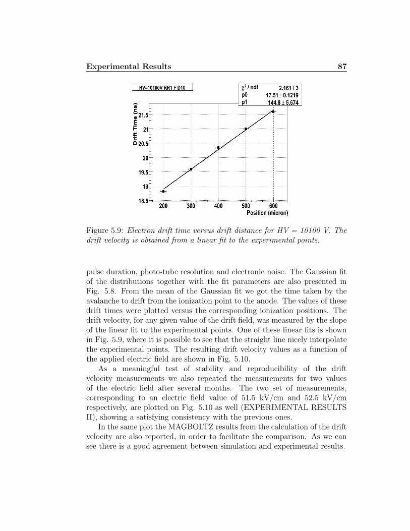
Experimental Results 87
Figure 5.9: Electron drift time versus drift distance for HV = 10100 V. Thedrift velocity is obtained from a linear fit to the experimental points.
pulse duration, photo-tube resolution and electronic noise. The Gaussian fitof the distributions together with the fit parameters are also presented inFig. 5.8. From the mean of the Gaussian fit we got the time taken by theavalanche to drift from the ionization point to the anode. The values of thesedrift times were plotted versus the corresponding ionization positions. Thedrift velocity, for any given value of the drift field, was measured by the slopeof the linear fit to the experimental points. One of these linear fits is shownin Fig. 5.9, where it is possible to see that the straight line nicely interpolatethe experimental points. The resulting drift velocity values as a function ofthe applied electric field are shown in Fig. 5.10.
As a meaningful test of stability and reproducibility of the driftvelocity measurements we also repeated the measurements for two valuesof the electric field after several months. The two set of measurements,corresponding to an electric field value of 51.5 kV/cm and 52.5 kV/cmrespectively, are plotted on Fig. 5.10 as well (EXPERIMENTAL RESULTSII), showing a satisfying consistency with the previous ones.
In the same plot the MAGBOLTZ results from the calculation of the driftvelocity are also reported, in order to facilitate the comparison. As we cansee there is a good agreement between simulation and experimental results.
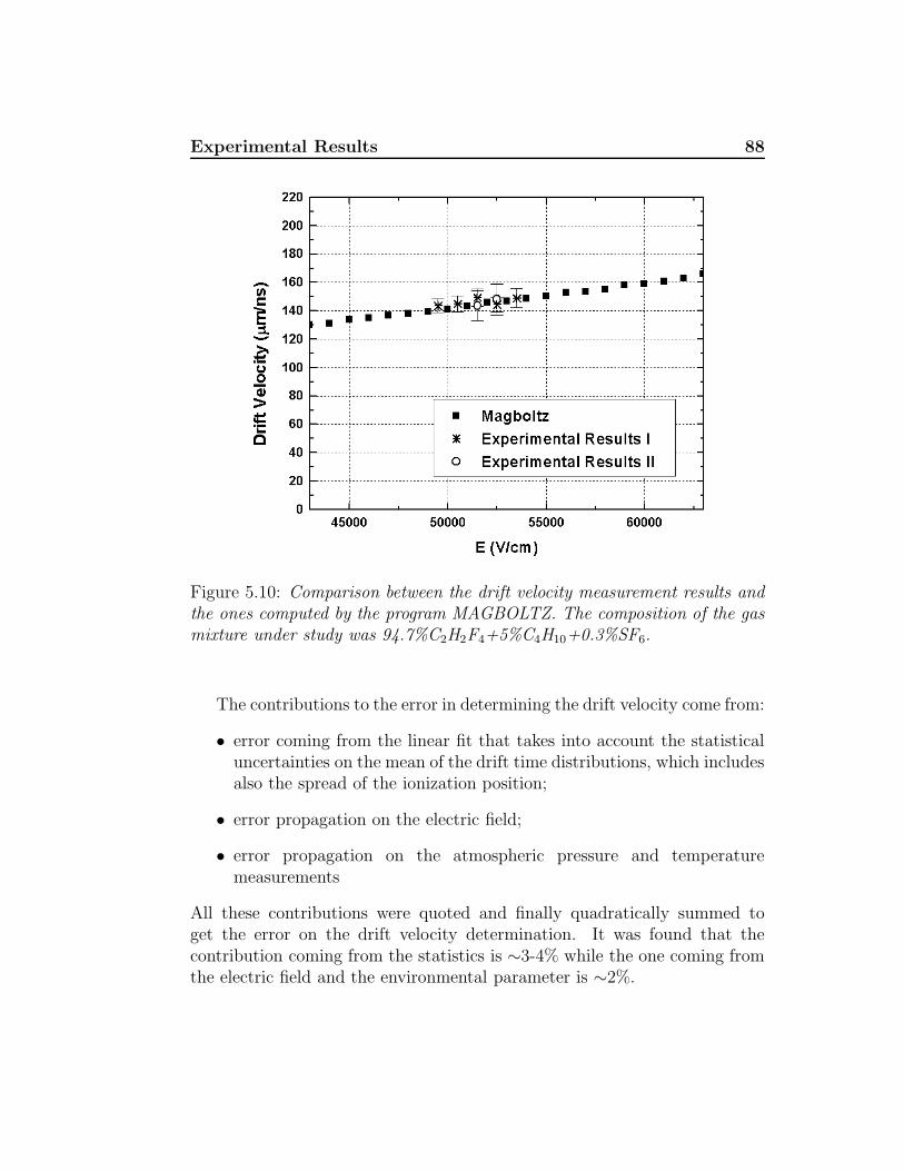
Experimental Results 88
Figure 5.10: Comparison between the drift velocity measurement results andthe ones computed by the program MAGBOLTZ. The composition of the gasmixture under study was 94.7%C2H2F4+5%C4H10+0.3%SF6.
The contributions to the error in determining the drift velocity come from:
• error coming from the linear fit that takes into account the statisticaluncertainties on the mean of the drift time distributions, which includesalso the spread of the ionization position;
• error propagation on the electric field;
• error propagation on the atmospheric pressure and temperaturemeasurements
All these contributions were quoted and finally quadratically summed toget the error on the drift velocity determination. It was found that thecontribution coming from the statistics is ∼3-4% while the one coming fromthe electric field and the environmental parameter is ∼2%.
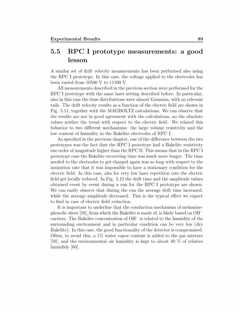
Experimental Results 89
5.5 RPC I prototype measurements: a good
lesson
A similar set of drift velocity measurements has been performed also usingthe RPC I prototype. In this case, the voltage applied to the electrodes hasbeen varied from 10500 V to 11100 V.
All measurements described in the previous section were performed for theRPC I prototype with the same laser setting described before. In particular,also in this case the time distributions were almost Gaussian, with no relevanttails. The drift velocity results as a function of the electric field are shown inFig. 5.11, together with the MAGBOLTZ calculations. We can observe thatthe results are not in good agreement with the calculations, no the absolutevalues neither the trend with respect to the electric field. We related thisbehavior to two different mechanisms: the large volume resistivity and thelow content of humidity in the Bakelite electrodes of RPC I.
As specified in the previous chapter, one of the difference between the twoprototypes was the fact that the RPC I prototype had a Bakelite resistivityone order of magnitude higher than the RPC II. This means that in the RPC Iprototype case the Bakelite recovering time was much more longer. The timeneeded to the electrodes to get charged again was so long with respect to theionization rate that it was impossible to have a stationary condition for theelectric field. In this case, also for very low laser repetition rate the electricfield get locally reduced. In Fig. 5.12 the drift time and the amplitude valuesobtained event by event during a run for the RPC I prototype are shown.We can easily observe that during the run the average drift time increased,while the average amplitude decreased. This is the typical effect we expectto find in case of electric field reduction.
It is important to underline that the conduction mechanism of melamine-phenolic sheet [58], from which the Bakelite is made of, is likely based on OH−
carriers. The Bakelite concentration of OH− is related to the humidity of thesurrounding environment and in particular condition can be very low (dryBakelite). In this case, the good functionality of the detector is compromised.Often, to avoid this, a 1% water vapor content is added to the gas mixture[59], and the environmental air humidity is kept to about 40 % of relativehumididy [60].
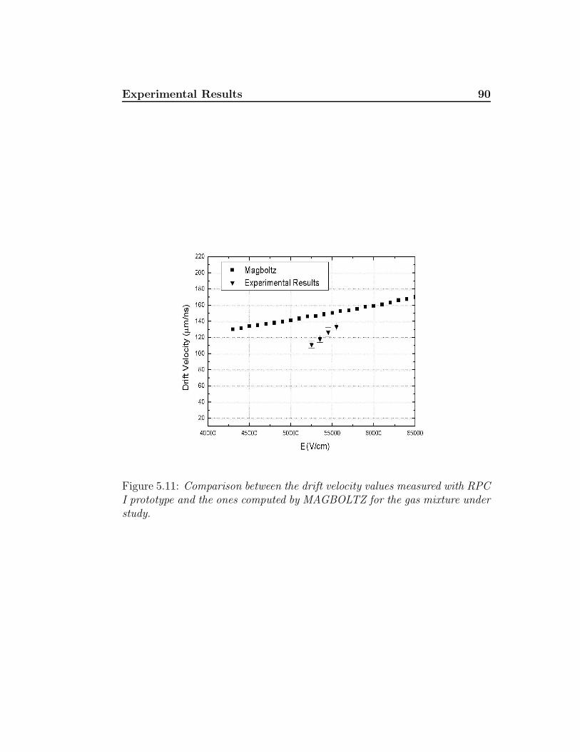
Experimental Results 90
Figure 5.11: Comparison between the drift velocity values measured with RPCI prototype and the ones computed by MAGBOLTZ for the gas mixture understudy.
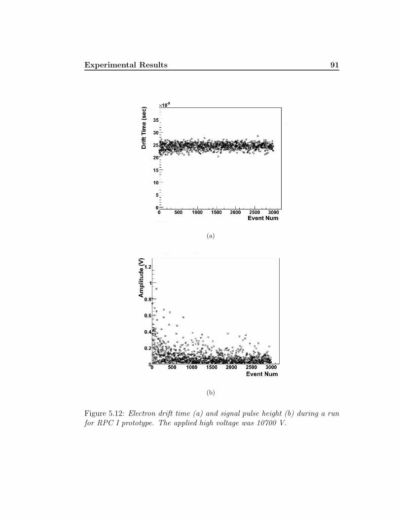
Experimental Results 91
(a)
(b)
Figure 5.12: Electron drift time (a) and signal pulse height (b) during a runfor RPC I prototype. The applied high voltage was 10700 V.
Experimental Results 92
5.6 Gas amplification Study
In literature several works are devoted to simulate the RPC behaviorchanging gas parameters and gap geometry. The main goal is to predict theRPC efficiency and time resolution in detecting minimum ionizing particles([1], [2], [61]). Some basic input parameters to the simulations are theelectron drift velocity and the effective Townsend coefficient. In particular,time resolution is related to the first parameter, and detection efficiency tothe second one.
In this section we report on the gas gain amplification and charge spectrameasurements in RPC II prototype. Similar measurements have been doneby several authors using cosmic rays ([2], [51], [62], [63]). In our setup wehad the unique feature to accomplish these studies in a simpler conditionthan with cosmic ray. In fact, the laser source generates electron avalanchein a well localized position, while with cosmic rays the signal is givenby the contribution of several avalanches initiated by primary ionizationelectron clusters. The clusters are released in the gap following the Poisson’sdistribution with average λ (≈ 9.5 clusters
mmfor ATLAS RPC gas mixture), thus
giving a large fluctuations in the readout signal just because the avalanchesstarting position fluctuates.
5.6.1 Saturated Avalanche Regime
In Fig. 5.4 (upper plot) the mean and the root mean square of the signal pulseheight have been shown with respect to the high voltage and for two differentaverage ionizations (µ ≈ 1 and 0.07). The mean pulse height increase withthe electric field exponentially for small value, but it begins to saturate (lineargrowth) for large electric field, just before the efficiency knee. The effectivegas amplification change from an exponential growth to a linear growth isattributed in literature [44] to space charge effects induced by the avalancheitself, which start to perturb the external electric field.
Following ref [48] we interpolated the gas amplification with respect tothe high voltage using the primitive of the Logistic function:
Q(V ) = Kln(1 + ea(V −V 0)) + Qth (5.6)
where K, a, V0 and Qth are fit parameters. We introduced the thresholdscharge Qth in order to take into account a positive shift in the average pulseheight induced by the software electronic noise suppression (see Sect. 4.4.4).
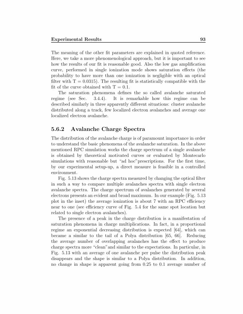
Experimental Results 93
The meaning of the other fit parameters are explained in quoted reference.Here, we take a more phenomenological approach, but it is important to seehow the results of our fit is reasonable good. Also the low gas amplificationcurve, performed in single ionization mode shows saturation effects (theprobability to have more than one ionization is negligible with an opticalfilter with T = 0.0315). The resulting fit is statistically compatible with thefit of the curve obtained with T = 0.1.
The saturation phenomena defines the so called avalanche saturatedregime (see Sec. 3.4.4). It is remarkable how this regime can bedescribed similarly in three apparently different situations: cluster avalanchedistributed along a track, few localized electron avalanches and average onelocalized electron avalanche.
5.6.2 Avalanche Charge Spectra
The distribution of the avalanche charge is of paramount importance in orderto understand the basic phenomena of the avalanche saturation. In the abovementioned RPC simulation works the charge spectrum of a single avalancheis obtained by theoretical motivated curves or evaluated by Montecarlosimulations with reasonable but “ad hoc”prescriptions. For the first time,by our experimental setup-up, a direct measure is feasible in a controlledenvironment.
Fig. 5.13 shows the charge spectra measured by changing the optical filterin such a way to compare multiple avalanches spectra with single electronavalanche spectra. The charge spectrum of avalanches generated by severalelectrons presents an evident and broad maximum. In our example (Fig. 5.13plot in the inset) the average ionization is about 7 with an RPC efficiencynear to one (see efficiency curve of Fig. 5.4 for the same spot location butrelated to single electron avalanches).
The presence of a peak in the charge distribution is a manifestation ofsaturation phenomena in charge multiplications. In fact, in a proportionalregime an exponential decreasing distribution is expected [64], which canbecame a similar to the tail of a Polya distribution [65, 66]. Reducingthe average number of overlapping avalanches has the effect to producecharge spectra more “clean”and similar to the expectations. In particular, inFig. 5.13 with an average of one avalanche per pulse the distribution peakdisappears and the shape is similar to a Polya distribution. In addition,no change in shape is apparent going from 0.25 to 0.1 average number of
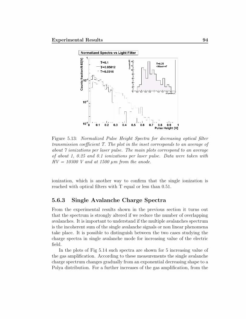
Experimental Results 94
Figure 5.13: Normalized Pulse Height Spectra for decreasing optical filtertransmission coefficient T. The plot in the inset corresponds to an average ofabout 7 ionizations per laser pulse. The main plots correspond to an averageof about 1, 0.25 and 0.1 ionizations per laser pulse. Data were taken withHV = 10300 V and at 1500 µm from the anode.
ionization, which is another way to confirm that the single ionization isreached with optical filters with T equal or less than 0.51.
5.6.3 Single Avalanche Charge Spectra
From the experimental results shown in the previous section it turns outthat the spectrum is strongly altered if we reduce the number of overlappingavalanches. It is important to understand if the multiple avalanches spectrumis the incoherent sum of the single avalanche signals or non linear phenomenatake place. It is possible to distinguish between the two cases studying thecharge spectra in single avalanche mode for increasing value of the electricfield.
In the plots of Fig 5.14 such spectra are shown for 5 increasing value ofthe gas amplification. According to these measurements the single avalanchecharge spectrum changes gradually from an exponential decreasing shape to aPolya distribution. For a further increases of the gas amplification, from the
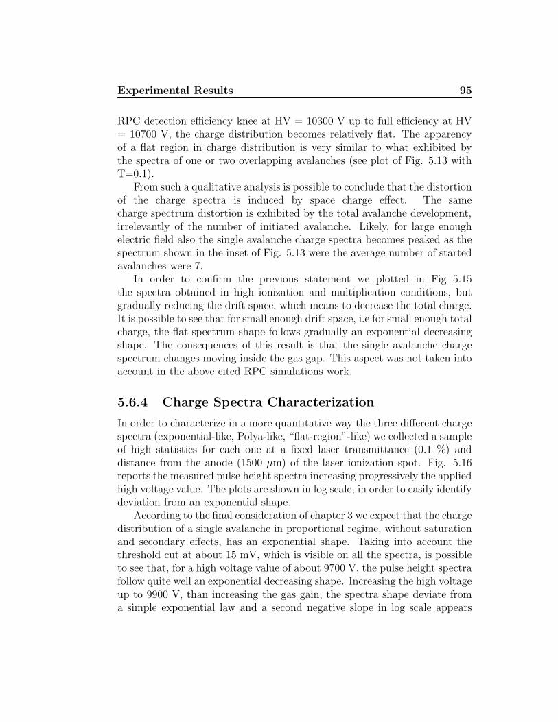
Experimental Results 95
RPC detection efficiency knee at HV = 10300 V up to full efficiency at HV= 10700 V, the charge distribution becomes relatively flat. The apparencyof a flat region in charge distribution is very similar to what exhibited bythe spectra of one or two overlapping avalanches (see plot of Fig. 5.13 withT=0.1).
From such a qualitative analysis is possible to conclude that the distortionof the charge spectra is induced by space charge effect. The samecharge spectrum distortion is exhibited by the total avalanche development,irrelevantly of the number of initiated avalanche. Likely, for large enoughelectric field also the single avalanche charge spectra becomes peaked as thespectrum shown in the inset of Fig. 5.13 were the average number of startedavalanches were 7.
In order to confirm the previous statement we plotted in Fig 5.15the spectra obtained in high ionization and multiplication conditions, butgradually reducing the drift space, which means to decrease the total charge.It is possible to see that for small enough drift space, i.e for small enough totalcharge, the flat spectrum shape follows gradually an exponential decreasingshape. The consequences of this result is that the single avalanche chargespectrum changes moving inside the gas gap. This aspect was not taken intoaccount in the above cited RPC simulations work.
5.6.4 Charge Spectra Characterization
In order to characterize in a more quantitative way the three different chargespectra (exponential-like, Polya-like, “flat-region”-like) we collected a sampleof high statistics for each one at a fixed laser transmittance (0.1 %) anddistance from the anode (1500 µm) of the laser ionization spot. Fig. 5.16reports the measured pulse height spectra increasing progressively the appliedhigh voltage value. The plots are shown in log scale, in order to easily identifydeviation from an exponential shape.
According to the final consideration of chapter 3 we expect that the chargedistribution of a single avalanche in proportional regime, without saturationand secondary effects, has an exponential shape. Taking into account thethreshold cut at about 15 mV, which is visible on all the spectra, is possibleto see that, for a high voltage value of about 9700 V, the pulse height spectrafollow quite well an exponential decreasing shape. Increasing the high voltageup to 9900 V, than increasing the gas gain, the spectra shape deviate froma simple exponential law and a second negative slope in log scale appears
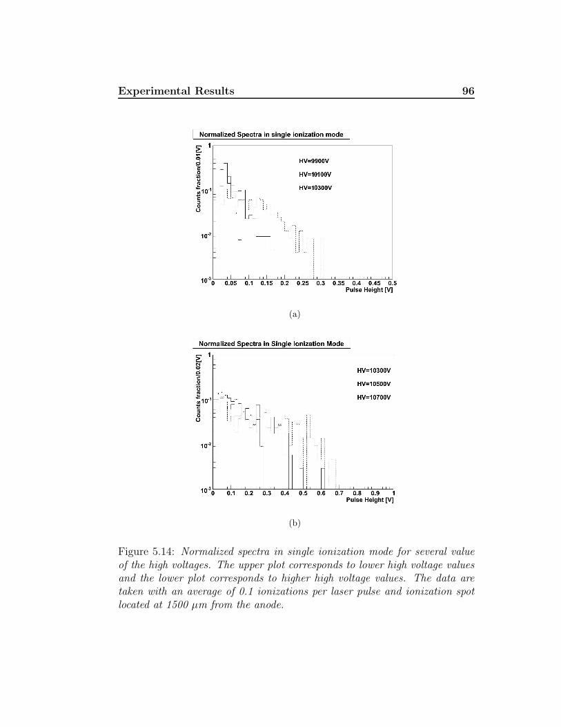
Experimental Results 96
(a)
(b)
Figure 5.14: Normalized spectra in single ionization mode for several valueof the high voltages. The upper plot corresponds to lower high voltage valuesand the lower plot corresponds to higher high voltage values. The data aretaken with an average of 0.1 ionizations per laser pulse and ionization spotlocated at 1500 µm from the anode.
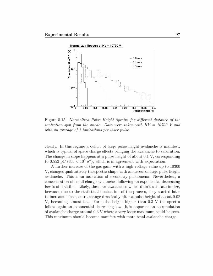
Experimental Results 97
Figure 5.15: Normalized Pulse Height Spectra for different distance of theionization spot from the anode. Data were taken with HV = 10700 V andwith an average of 1 ionizations per laser pulse.
clearly. In this regime a deficit of large pulse height avalanche is manifest,which is typical of space charge effects bringing the avalanche to saturation.The change in slope happens at a pulse height of about 0.1 V, correspondingto 0.552 pC (3.4 × 10⁶ e−), which is in agreement with expectation.
A further increase of the gas gain, with a high voltage value up to 10300V, changes qualitatively the spectra shape with an excess of large pulse heightavalanche. This is an indication of secondary phenomena. Nevertheless, aconcentration of small charge avalanches following an exponential decreasinglaw is still visible. Likely, these are avalanches which didn’t saturate in size,because, due to the statistical fluctuation of the process, they started laterto increase. The spectra change drastically after a pulse height of about 0.08V, becoming almost flat. For pulse height higher than 0.3 V the spectrafollow again an exponential decreasing law. It is apparent an accumulationof avalanche charge around 0.3 V where a very loose maximum could be seen.This maximum should become manifest with more total avalanche charge.
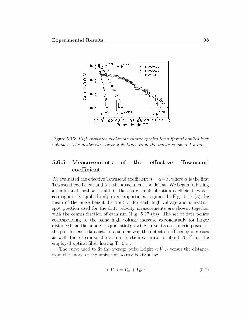
Experimental Results 98
Figure 5.16: High statistics avalanche charge spectra for different applied highvoltages. The avalanche starting distance from the anode is about 1.5 mm.
5.6.5 Measurements of the effective Townsendcoefficient
We evaluated the effective Townsend coefficient η = α−β, where α is the firstTownsend coefficient and β is the attachment coefficient. We began followinga traditional method to obtain the charge multiplication coefficient, whichcan rigorously applied only in a proportional regime. In Fig. 5.17 (a) themean of the pulse height distribution for each high voltage and ionizationspot position used for the drift velocity measurements are shown, togetherwith the counts fraction of each run (Fig. 5.17 (b)). The set of data pointscorresponding to the same high voltage increase exponentially for largerdistance from the anode. Exponential growing curve fits are superimposed onthe plot for each data set. In a similar way the detection efficiency increasesas well, but of course the counts fraction saturate to about 70 % for theemployed optical filter having T=0.1 .
The curve used to fit the average pulse height < V > versus the distancefrom the anode of the ionization source is given by:
< V >= Vth + V0eηx (5.7)
Experimental Results 99
where the parameter Vth takes into account the threshold cut in pulseheight, V0 is the average pulse height at position x = 0 and η is the effectivecharge multiplication coefficient. The coefficient η extracted with such amethod is relatively insensitive to the electric field (see Fig. 5.18 method I).Moreover, its value is about half the effective Townsend coefficient evaluatedby MAGBOLTZ. Of course, we are in presence of a saturation effect relatedto the space charge. Although the average pulse height increases with theelectric field the growth is not so fast as expected. In Fig. 5.17 (a) each datapoint was labeled with the corresponding type of charge spectrum obtainedexperimentally. It is possible to notice that all curves go through twotransitions: the first one to about 0.04 V of average pulse height (exponentialto Polya-like spectrum) and the second one to about 0.08 V of average pulseheight (Polya to “flat-region”spectrum).
The second method to extract the parameter η, to compare withMAGBOLTZ calculations, consisted into extract the gas gain in conditionwhere avalanche saturation doesn’t occur by fitting the pulse heightdistribution. This corresponds to use the pulse height distributionscorresponding to the data points of Fig. 5.17(a) labeled with “exp”.Usually, for each high voltage, there were two position whose data showed anexponential-like spectrum, then in the plot of Fig. 5.18 the results of methodII are kept separated for the two positions.
These data points are characterized by small amplitudes and the accuracyin pulse height determination is unsatisfactory. As explained in [66], [67]and [44] a better estimation of the average charge is measuring the slope insemilogarithmic scale of the normalized spectrum. In fact, in this case thespectrum is ≈ q
<q>e−
q
<q> and from the slope you can extract < q > which isrelated to η by the Townsend multiplication law: < q >= eηx. The absoluteposition x of the ionization spot from the anode is known with an uncertaintyof about ±0.1 mm and this introduce a systematic eror in the measurementsnot repoted in the plot. The coefficient η extracted with this method isconsistent with the value calculated by MAGBOLTZ (see Fig. 5.18 methodII).
5.6.6 Avalanche Charge Spectra with no SF6
It was instructive to study the charge spectra of the RPC gas mixturewithout SF6 in order to learn more about streamer suppressions, even ifonly qualitative considerations have been drawn out.
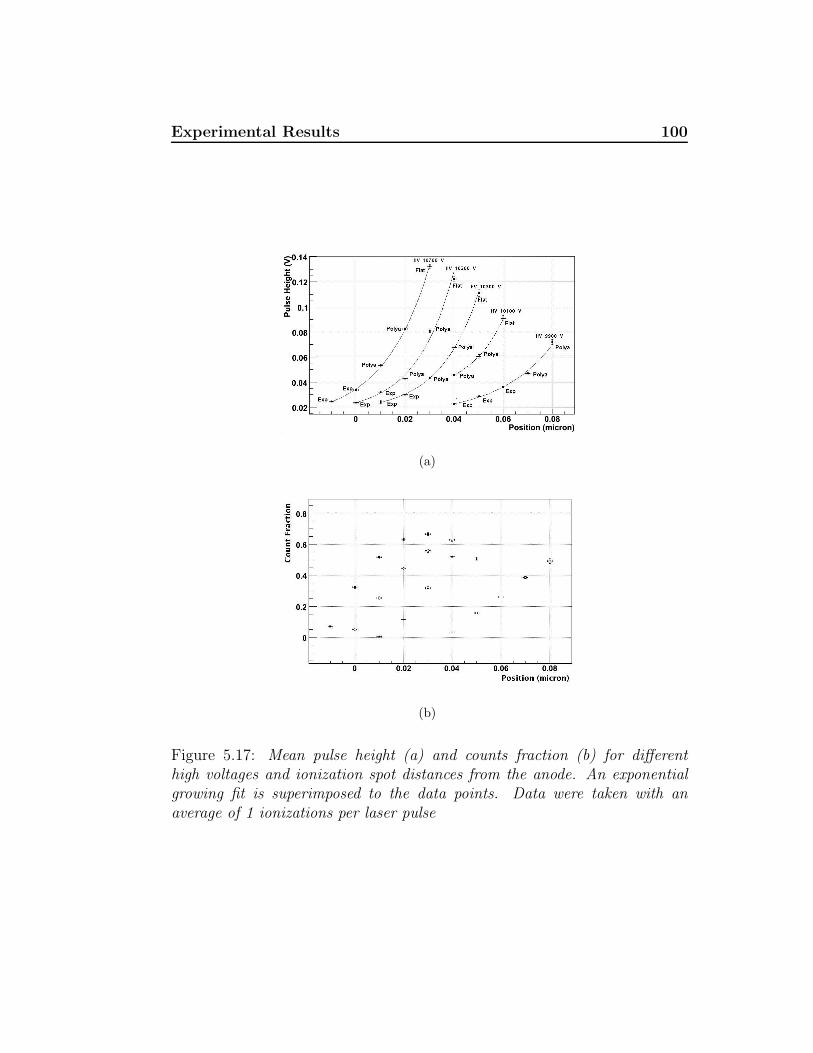
Experimental Results 100
(a)
(b)
Figure 5.17: Mean pulse height (a) and counts fraction (b) for differenthigh voltages and ionization spot distances from the anode. An exponentialgrowing fit is superimposed to the data points. Data were taken with anaverage of 1 ionizations per laser pulse
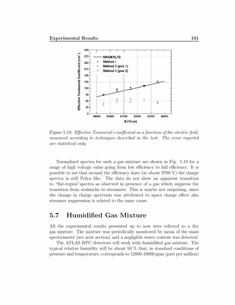
Experimental Results 101
Figure 5.18: Effective Townsend’s coefficient as a function of the electric field,measured according to techniques described in the text. The error reportedare statistical only.
Normalized spectra for such a gas mixture are shown in Fig. 5.19 for arange of high voltage value going from low efficiency to full efficiency. It ispossible to see that around the efficiency knee (at about 9700 V) the chargespectra is still Polya like. The data do not show an apparent transitionto “flat-region”spectra as observed in presence of a gas which suppress thetransition from avalanche to streamers. This is maybe not surprising, sincethe change in charge spectrum was attributed to space charge effect alsostreamer suppression is related to the same cause.
5.7 Humidified Gas Mixture
All the experimental results presented up to now were referred to a drygas mixture. The mixture was periodically monitored by mean of the massspectrometer (see next section) and a negligible water content was detected.
The ATLAS RPC detectors will work with humidified gas mixture. Thetypical relative humidity will be about 50 % that, in standard conditions ofpressure and temperature, corresponds to 12000-18000 ppm (part per million)
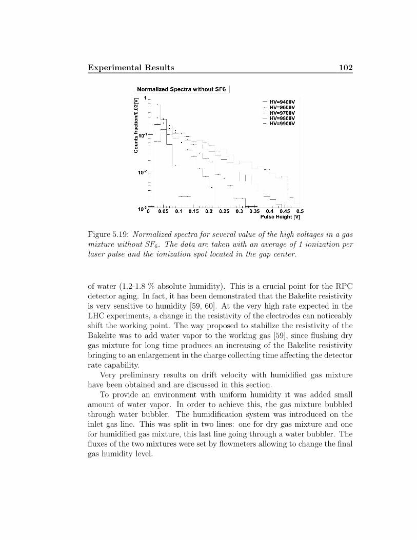
Experimental Results 102
Figure 5.19: Normalized spectra for several value of the high voltages in a gasmixture without SF6. The data are taken with an average of 1 ionization perlaser pulse and the ionization spot located in the gap center.
of water (1.2-1.8 % absolute humidity). This is a crucial point for the RPCdetector aging. In fact, it has been demonstrated that the Bakelite resistivityis very sensitive to humidity [59, 60]. At the very high rate expected in theLHC experiments, a change in the resistivity of the electrodes can noticeablyshift the working point. The way proposed to stabilize the resistivity of theBakelite was to add water vapor to the working gas [59], since flushing drygas mixture for long time produces an increasing of the Bakelite resistivitybringing to an enlargement in the charge collecting time affecting the detectorrate capability.
Very preliminary results on drift velocity with humidified gas mixturehave been obtained and are discussed in this section.
To provide an environment with uniform humidity it was added smallamount of water vapor. In order to achieve this, the gas mixture bubbledthrough water bubbler. The humidification system was introduced on theinlet gas line. This was split in two lines: one for dry gas mixture and onefor humidified gas mixture, this last line going through a water bubbler. Thefluxes of the two mixtures were set by flowmeters allowing to change the finalgas humidity level.
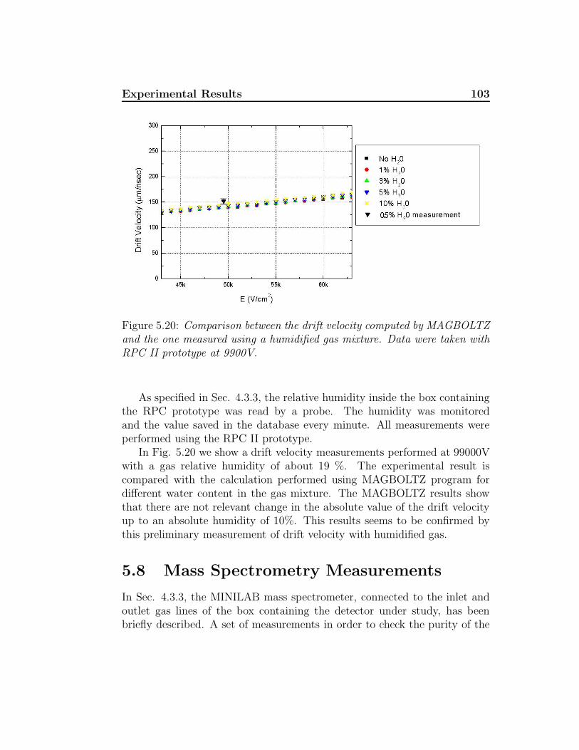
Experimental Results 103
Figure 5.20: Comparison between the drift velocity computed by MAGBOLTZand the one measured using a humidified gas mixture. Data were taken withRPC II prototype at 9900V.
As specified in Sec. 4.3.3, the relative humidity inside the box containingthe RPC prototype was read by a probe. The humidity was monitoredand the value saved in the database every minute. All measurements wereperformed using the RPC II prototype.
In Fig. 5.20 we show a drift velocity measurements performed at 99000Vwith a gas relative humidity of about 19 %. The experimental result iscompared with the calculation performed using MAGBOLTZ program fordifferent water content in the gas mixture. The MAGBOLTZ results showthat there are not relevant change in the absolute value of the drift velocityup to an absolute humidity of 10%. This results seems to be confirmed bythis preliminary measurement of drift velocity with humidified gas.
5.8 Mass Spectrometry Measurements
In Sec. 4.3.3, the MINILAB mass spectrometer, connected to the inlet andoutlet gas lines of the box containing the detector under study, has beenbriefly described. A set of measurements in order to check the purity of the
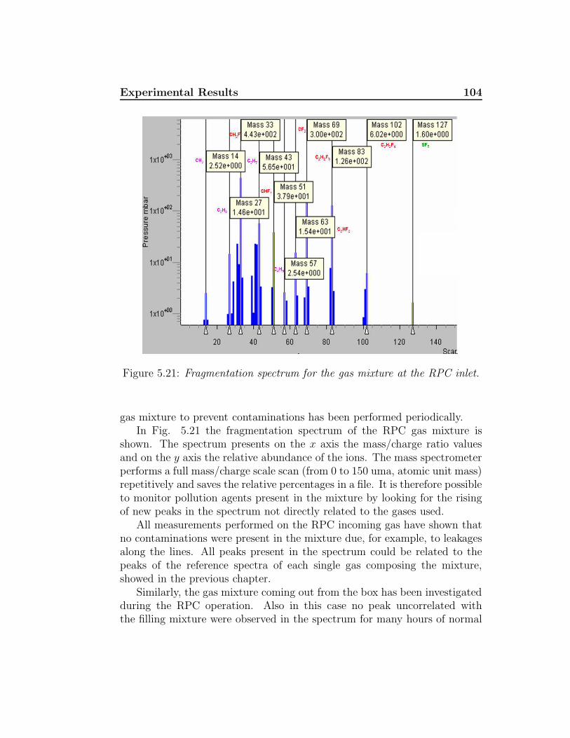
Experimental Results 104
Figure 5.21: Fragmentation spectrum for the gas mixture at the RPC inlet.
gas mixture to prevent contaminations has been performed periodically.In Fig. 5.21 the fragmentation spectrum of the RPC gas mixture is
shown. The spectrum presents on the x axis the mass/charge ratio valuesand on the y axis the relative abundance of the ions. The mass spectrometerperforms a full mass/charge scale scan (from 0 to 150 uma, atomic unit mass)repetitively and saves the relative percentages in a file. It is therefore possibleto monitor pollution agents present in the mixture by looking for the risingof new peaks in the spectrum not directly related to the gases used.
All measurements performed on the RPC incoming gas have shown thatno contaminations were present in the mixture due, for example, to leakagesalong the lines. All peaks present in the spectrum could be related to thepeaks of the reference spectra of each single gas composing the mixture,showed in the previous chapter.
Similarly, the gas mixture coming out from the box has been investigatedduring the RPC operation. Also in this case no peak uncorrelated withthe filling mixture were observed in the spectrum for many hours of normal

Experimental Results 105
operation. than 8 hours of detector operation in normal condition. Thistechnique could be actually used to monitor aging effects in RPC or the gasmixture in particular conditions, like high ionization rate for long period,atc.
In Fig. 5.22 (a) the fragmentation spectrum of the Nitrogen used for thelaser is shown. The spectrum is perfectly compatible with the reference onefrom NIST (Fig. 5.22)(b) but it shows a peak at 18 uma related with thepresence of water since to supply the laser gas plastic tubes, absorbing water,instead of stain-steel tubes have been used.
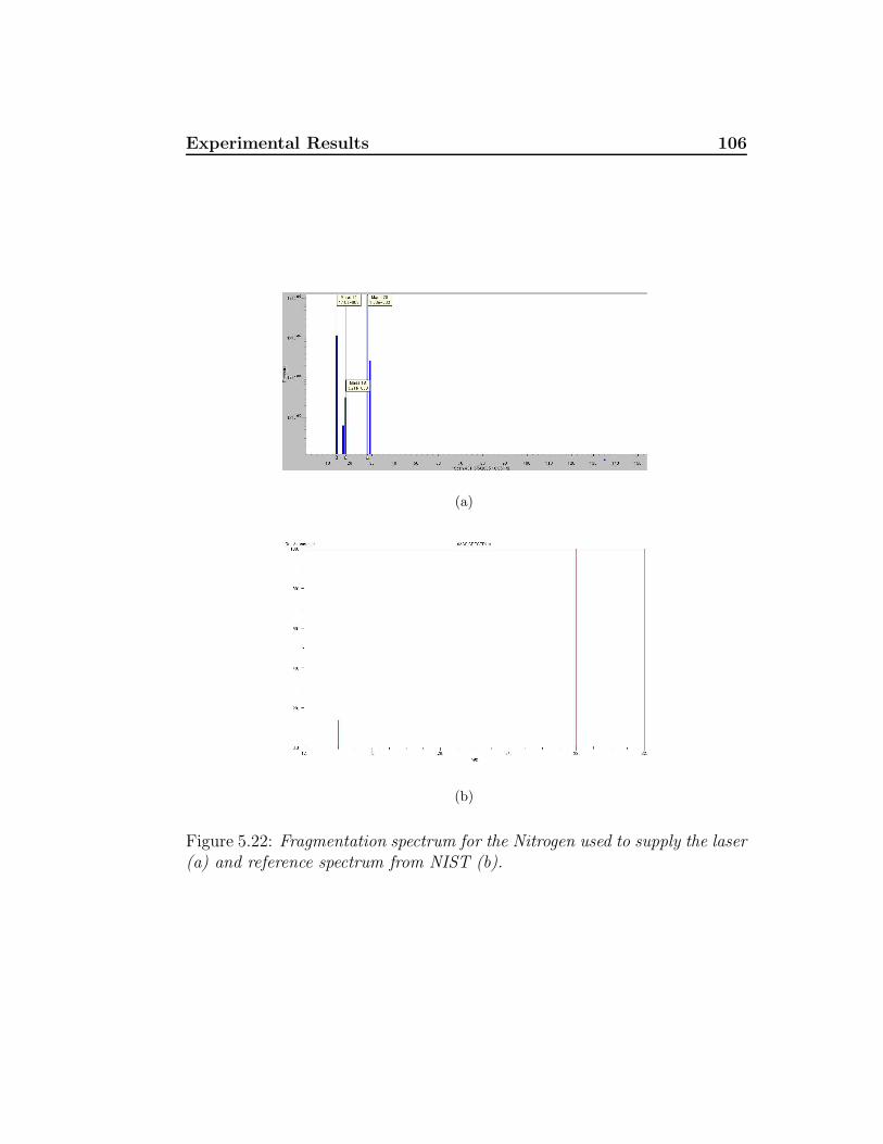
Experimental Results 106
(a)
(b)
Figure 5.22: Fragmentation spectrum for the Nitrogen used to supply the laser(a) and reference spectrum from NIST (b).
Conclusions
In this thesis extensive studies of electron transport and amplificationproperties in the gas mixture filling RPC ATLAS-like have been reportedas a function of the electric field in saturated avalanche regime.
Measurements have been performed by using an existing facilityexploiting a UV laser source to induce ionization in gas detectros, after acomplete re-design of DAQ and DCS system and analysis software.
Results of drift velocity and gas amplification, for different values of theelectric field in the mixture: 94.7% C2H2F4 + 5% C4H10 + 0.3% SF6 havebeen obtained. A small size (10×20 cm2) ATLAS-like RPC, having 2 mm gasgap thickness and inner surface linseed-oil-treated Bakelite electrodes with1.71 × 1010 Ω cm volume resistivity has been used as active detectror.
Electron drift velocities have been compared to the values calculated bythe program MAGBOLTZ and a satisfying agreement was found.
The evaluation of the gas amplification was found to be complicatedby space charge effects typical of the RPC operating regime of saturatedavalanches. We found that the charge spectrum distribution follows anexponential decreasing curve ( 1
<q>e−
q
<q> ) for electron avalanche charges less
than ∼106e−, while starts to saturate assuming a Polya-like curve shape([ q
<q>(1+θ)]θe−(1+θ) q
<q> ) for larger amount of charge. Further increase of theelectron avalanche charge distorts completely the charge spectrum, whichexhibits a relatively flat region with a possible broad maximum.
The average signal pulse-height was measured for different distances fromthe anode of the laser spot and for several values of the electric field.An exponential growth of the average pulse-height was observed with thedistance from the anode. The effective Townsend’s coefficient, defined as thedifference between the Townsend’s coefficient and the electron attachmentcoefficient, was evaluated, as a function of the electric field, at distancessmall enough from the anode, for which an exponential behaviour of the

Conclusions 108
charge spectra was still reliable, thus avoiding saturation effects. Theobtained effective Townsend’s coefficients agree with the calculations fromMAGBOLTZ.
Finally, a very preliminary drift velocity measurements has beenperformed with humidified gas mixture. This was performed in order tosetup all devices for collecting systematic measurements with humidify gasmixture in the near future.
Appendix A
Special ATLAS RPC Chambertests at CERN
The barrel muon spectrometer is made of 680 stations arranged radially atabout 5, 7.5 and 10 meters from the beam line. Innermost stations are madeof two “multi-layers”each housing four layers of MDT tubes. Middle stationsare made of two multi-layers of 3 layers each of MDT tubes placed betweentwo RPC planes (so colled Pivot and Low Pt planes). Outer stations aremade of two multi-layers of 3 layers each of MDT tubes and one RPC plane(High Pt plane).
Muon stations are organized in 16 geometrical sectors along the azimuthalangle, following the eightfold layout symmetry of the magnetic barrel toroidcoils. More precisely, the 16 sectors are subdivided in 8 small and 8 large,according to the position with respect to superconducting coils.
Fig. A.1 shows a typical middle muon station of a small sector. Theregions around the coil ribs have a loss of muon coverage of ∼ 3% of the fullbarrel acceptance for muons coming from the interaction region. This meansa loss of efficiency of about 12 % for a full reconstructed four-muon decay ofthe Higgs boson. In ATLAS it has been decided to recover this acceptanceloss by building special RPC units to be placed around the rib coils. Thename “special”is referred to the fact that these RPC units are not joinedwith the corresponding high precision detectors.
In Fig. A.1 is possible to see how the special RPC units are mounted indoublets on aluminum frames and positioned on the rib coil by adjustablebrackets. There are two typologies of chambers, S2 units (about 30×100cm2) and S3 (about 60×100 cm2). Both units have holes to allow the passage
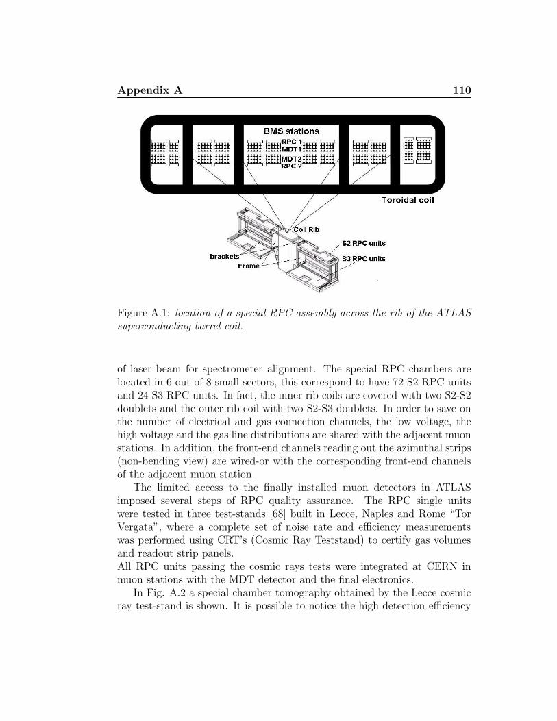
Appendix A 110
Figure A.1: location of a special RPC assembly across the rib of the ATLASsuperconducting barrel coil.
of laser beam for spectrometer alignment. The special RPC chambers arelocated in 6 out of 8 small sectors, this correspond to have 72 S2 RPC unitsand 24 S3 RPC units. In fact, the inner rib coils are covered with two S2-S2doublets and the outer rib coil with two S2-S3 doublets. In order to save onthe number of electrical and gas connection channels, the low voltage, thehigh voltage and the gas line distributions are shared with the adjacent muonstations. In addition, the front-end channels reading out the azimuthal strips(non-bending view) are wired-or with the corresponding front-end channelsof the adjacent muon station.
The limited access to the finally installed muon detectors in ATLASimposed several steps of RPC quality assurance. The RPC single unitswere tested in three test-stands [68] built in Lecce, Naples and Rome “TorVergata”, where a complete set of noise rate and efficiency measurementswas performed using CRT’s (Cosmic Ray Teststand) to certify gas volumesand readout strip panels.All RPC units passing the cosmic rays tests were integrated at CERN inmuon stations with the MDT detector and the final electronics.
In Fig. A.2 a special chamber tomography obtained by the Lecce cosmicray test-stand is shown. It is possible to notice the high detection efficiency
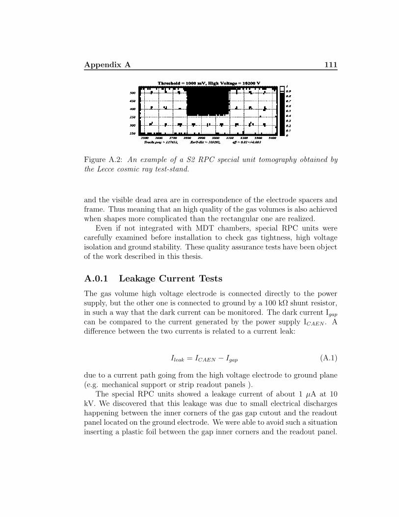
Appendix A 111
Figure A.2: An example of a S2 RPC special unit tomography obtained bythe Lecce cosmic ray test-stand.
and the visible dead area are in correspondence of the electrode spacers andframe. Thus meaning that an high quality of the gas volumes is also achievedwhen shapes more complicated than the rectangular one are realized.
Even if not integrated with MDT chambers, special RPC units werecarefully examined before installation to check gas tightness, high voltageisolation and ground stability. These quality assurance tests have been objectof the work described in this thesis.
A.0.1 Leakage Current Tests
The gas volume high voltage electrode is connected directly to the powersupply, but the other one is connected to ground by a 100 kΩ shunt resistor,in such a way that the dark current can be monitored. The dark current Igap
can be compared to the current generated by the power supply ICAEN . Adifference between the two currents is related to a current leak:
Ileak = ICAEN − Igap (A.1)
due to a current path going from the high voltage electrode to ground plane(e.g. mechanical support or strip readout panels ).
The special RPC units showed a leakage current of about 1 µA at 10kV. We discovered that this leakage was due to small electrical dischargeshappening between the inner corners of the gas gap cutout and the readoutpanel located on the ground electrode. We were able to avoid such a situationinserting a plastic foil between the gap inner corners and the readout panel.
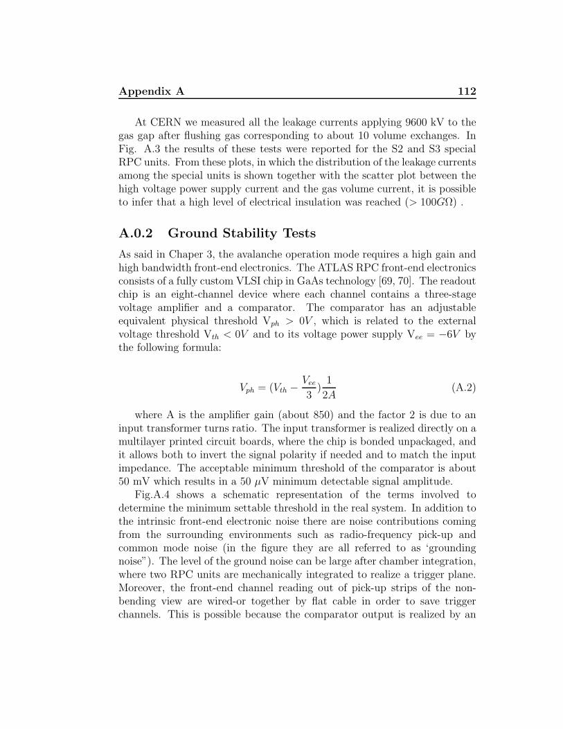
Appendix A 112
At CERN we measured all the leakage currents applying 9600 kV to thegas gap after flushing gas corresponding to about 10 volume exchanges. InFig. A.3 the results of these tests were reported for the S2 and S3 specialRPC units. From these plots, in which the distribution of the leakage currentsamong the special units is shown together with the scatter plot between thehigh voltage power supply current and the gas volume current, it is possibleto infer that a high level of electrical insulation was reached (> 100GΩ) .
A.0.2 Ground Stability Tests
As said in Chaper 3, the avalanche operation mode requires a high gain andhigh bandwidth front-end electronics. The ATLAS RPC front-end electronicsconsists of a fully custom VLSI chip in GaAs technology [69, 70]. The readoutchip is an eight-channel device where each channel contains a three-stagevoltage amplifier and a comparator. The comparator has an adjustableequivalent physical threshold Vph > 0V , which is related to the externalvoltage threshold Vth < 0V and to its voltage power supply Vee = −6V bythe following formula:
Vph = (Vth −Vee
3)
1
2A(A.2)
where A is the amplifier gain (about 850) and the factor 2 is due to aninput transformer turns ratio. The input transformer is realized directly on amultilayer printed circuit boards, where the chip is bonded unpackaged, andit allows both to invert the signal polarity if needed and to match the inputimpedance. The acceptable minimum threshold of the comparator is about50 mV which results in a 50 µV minimum detectable signal amplitude.
Fig.A.4 shows a schematic representation of the terms involved todetermine the minimum settable threshold in the real system. In addition tothe intrinsic front-end electronic noise there are noise contributions comingfrom the surrounding environments such as radio-frequency pick-up andcommon mode noise (in the figure they are all referred to as ‘groundingnoise”). The level of the ground noise can be large after chamber integration,where two RPC units are mechanically integrated to realize a trigger plane.Moreover, the front-end channel reading out of pick-up strips of the non-bending view are wired-or together by flat cable in order to save triggerchannels. This is possible because the comparator output is realized by an
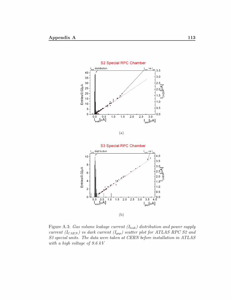
Appendix A 113
(a)
(b)
Figure A.3: Gas volume leakage current (Ileak) distribution and power supplycurrent (ICAEN) vs dark current (Igap) scatter plot for ATLAS RPC S2 andS3 special units. The data were taken at CERN before installation in ATLASwith a high voltage of 9.6 kV
Appendix A 114
single ended open emitter configuration, which can drive up to few meter longflat cable. Unfortunately, the one meter long flat cable wired-or solutionintroduce a negligible grounding noise only if the inner single RPC unitgrounding is robust. For this reason, a grounding stability test in a wired-orconfiguration before installation was necessary.
We did these grounding tests on special RPC units by realizing an ‘adhoc” wired-or configuration between two units and employing the real triggerelectronics to terminate the output channels.
The grounding test consisted in the following steps:1) Set the external threshold to -1.8 V, below the noise level. In this
situation all the comparators are always turned on and drawing current,because of the open emitter output configuration.
2) Increase the external threshold at step of 0.1 V and record the Vth
value at which the excess of drawn current disappears. This mean that thecomparators stop to fire.
The Vth value at which the electronics stop to fire is an indication of thegrounding stability reached by the chambers. We tested in such a way all the96 special RPC units and we obtained that a the S2 units recover a stablesituation at Vth ≈ 1.7V . A value of about 1.5 V was instead obtained forthe S3 units. We had to open and fix only 3 units, because we found a toolow margin stability.
The ATLAS RPC detectors are fully efficient at Vth=-1V for minimumionization particle (see Fig. A.4). Nevertheless, to have a large safety margin,in view of possible noise in the experiment and during p-p collisions, a verystringent test were requiring a Vth recovery value not worse than 1.3 V. Thespecial RPC units are well within the requirements.
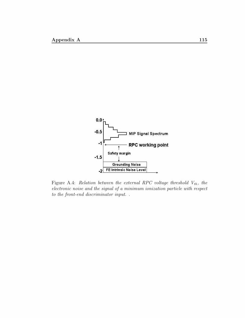
Appendix A 115
Figure A.4: Relation between the external RPC voltage threshold Vth, theelectronic noise and the signal of a minimum ionization particle with respectto the front-end discriminator input. .

Bibliografy
[1] W. Riegler et al., Nucl. Instr. and Meth. A500 (2003) 144-162.
[2] M. Abbrescia et al., Nucl. Instr. and Meth. A431 (1999) 413-427.
[3] S. Biagi, Nucl. Instr. and Meth. A421 (1999) 234-240.
[4] S. Biagi, MAGBOLTZ, program to computegas properties, version 7.8,,CERN.
[5] LHC Technical Desing Report,http://ab-div.web.ch/ab-div/Publications/LHC-DesignReport.html
[6] F. Halzen & A.D. Martin, Quarks and Leptons: an introductory coursein modern particle physics, John Wiley & Sons, USA (1984).
[7] D. Treille, Physics Reports 403-404 (2004) 221-239.
[8] G. Altarelli, M.W. Grunewald, Physics Reports 403-404 (2004) 189-201.
[9] H.E. Haber, G.L. Kane, Phys. Rep. C117 (1985) 75.
[10] S. Abdullin, C. Kao and N. Stepanof, Univeristy of Rochester UR-1475,July1996.
[11] K.D. Lane hep-ph/9605257 (1996).
[12] S. Coleman, J. Mandula; Phys. Rev. 159, 1251 (1967).
[13] L. Alvarez-Gaume, J. Polchinski and M.B. Wise, Nucl. Phys. B221(1983) 495.
[14] M. Dine, W. Fischler and M. Srednicki, Nucl. Phys. B189, (1981) 575.
Bibliography 117
[15] L.Randall and R. Sundrum, Nucl. Phys. B557, (1999) 79.
[16] ATLAS Collaboration. ATLAS Technical Desing Report.http://atlas.web.cern.ch/Atlas/Welcome.html
[17] I. Hinchliffe, F.E. Paige , Phys. Rev. D 60, 095002.
[18] W.M. Yao et al. (Particle Data Group); J. Phys. G33 1 (2006).
[19] G.F. Giudice, R. Rattazzi; Phys. Rep. 322 (1999) 419.
[20] CMS Collaboration. CMS Technical Desing Report.http://cmsdoc.cern.ch/outreach/
[21] LHCb Collaboration. LHCb Technical Desing Report.http://lhcb.web.cern.ch/lhcb/
[22] ALICE Collaboration. ALICE Technical Desing Report.http://alice.web.cern.ch/Alice/Alicenew/
[23] N. Ellis, T.S. Virdee, Experimental challengesnin high luminositycollider physics. Ann. Rev. Nucl. Part. Sci. 44 (1994) 609.
[24] I. Foster and C. Kesselman (editors), The Grid: Blueprint for a FutureComputing Infrastructure Morgan Kaufmann Publishers, USA, 1999.
[25] http://lcg.web.cern.ch/LCG.
[26] ATLAS Inner Detector Comunity In-ner Detector Technical Desing Reporthttp://atlas.web.cern.ch/Atlas/GROUPS/INNER DETECTOR/TDR/tdr.html
[27] ATLAS Collaboration. ATLAS Muon Spectrometer Technical DesingReport. CERN/LHCC/97-22, ATLAS TDR 10, (1997).
[28] ATLAS Collaboration. ATLAS Detector and Physics PerformanceTechnical Desing Report. CERN/LHCC/99-124 (1999).
[29] W. Blum,ATLAS Internal Note, MUON-NO-24 (1993).
[30] D. Drakoulakos et al., XTOM2, Stereo-Measurements of the MDT MuonChambers using high precision X-ray Tomograph. ATLAS Note, MUON-NO-155 (1997).
Bibliography 118
[31] V. Paschhoff and M. Spegel, Aging studies for the ATLAS MDTs usingAr-CO2,ATLAS Note, ATL-MUON-2000-004 (2000).
[32] H. Groenstege, The RASNIK/CCD 3D alignment system. ATL-MUON-94-063.
[33] E. Duchovni et al. Possible Utilization of Thin-Gap-Chambers in theATLAS Muon System; ATLA-MUON-93-023
[34] K. Nagai, Nucl. Instr. Meth. A 384 (1996) 219.
[35] V. Smakhtin, Nucl. Instr. Meth. A 494 (2002) 500-503.
[36] R. Santonico and R. Cardarelli, Nucl. Instr. Meth. 187 (1981) 377-380.
[37] R. Santonico and R. Cardarelli, Nucl. Instr. Meth. A 263 (1988) 20-25.
[38] W. Blum and L. Rolandi, Particle Detection with Drift Chambers,Springer, 1993.
[39] V.V. Parkhochuck et al., Nucl. Instr. Meth.93 (1971) 269.
[40] H.A. Bethe, Z. Physik, 76:293, 1932.
[41] K. Hagiwara et al., Physical Review. D 66 (2002).
[42] Particle Data Group, http://pdg.lbl.gov
[43] L.D. Landau, J. Exp. Phys. (URSS), 8:201, 1944.
[44] H. Raether, Electron Avalanches and Breakdown in Gaseous, LondonButterworths, 1964.
[45] K. Kleinknecht Detectors for Particle Radiation, Cambridge UniversityPress, 1986.
[46] S. Ramo, Proc. IRE 27 (1939) 584.
[47] W. Riegler, Nucl. Instr. and Meth. A491:258-271, 2002.
[48] G. Aielli et al., Nucl. Instr. and Meth. A508:6-13, 2003.
[49] H. Genz, Nucl. Instr. and Meth. 112 (1973) 83.
Bibliography 119
[50] A. Colucci et al, Nucl. Instr. and Meth. A425:84-91, 1999.
[51] P. Camarri et al, Nucl. Instr. and Meth. A414:317-324, 1998.
[52] V. Golovatyuk et al, Nucl. Instr. and Meth. A461:96-97, 2001.
[53] H.J. Hilke, Nucl. Instr. and Meth. A252:169-179, 1986.
[54] E. Marotta et al., J. Mass Sprctrom. 2004; 39:791-801.
[55] NIST Chemistry WebBook, Standard Reference Database Number, 69,June 2005. http://webbook.nist.gov/chemistry.
[56] http://www.caen.it/nuclear/products.php.
[57] B. Rene, http://root.cern.ch
[58] C. Chiri, Tesi di Lauea, Universita’ di Lecce.
[59] I. Crotty et al., Nucl. Instr. and Meth. A360 (1995) 512-520.
[60] G. Aielli et al., IEEE Trans. Nucl. Sci. 53: 567-571, 2006.
[61] E.C. Zeballos et al., Nucl. Instr. and Meth. A396 (1997) 93-102.
[62] V.V. Ammosov et al., Comparison between 2mm and 3.5 mm gap RPCsoperated at low gas gain, September 1996, Protvino, Russia.
[63] M.G. Alviggi et al., ATLAS Internal Note MUON-NO-131, 1 October1996.
[64] F. Sauli, Nucl. Instr. and Meth. A553 (2005) 18-24.
[65] J. Va’vra, Nucl. Instr. and Meth. A371 (1996) 35-56.
[66] A. Buzulutskov et al., Nucl. Instr. and Meth. A443 (2000) 164-180.
[67] A. Bondar et al., Nucl. Instr. and Meth. A574 (2007) 493-299.
[68] A. Aloisio et al., Nucl. Instr. and Meth. A 435 (2004) 256-271.
[69] G.Aielli et al., Nucl. Instrum. and Meth. A409 (1998) 291-293.
[70] F. Giannini et al., Nucl. Instr. and Meth. A432 (1999) 440.