UNIVERSITÀ DEGLI STUDI DI PADOVA

Dipartimento di Scienze Economiche “Marco Fanno”

ESTIMATING A NKBC MODEL FOR THE U.S. ECONOMY WITH MULTIPLE FILTERS

EFREM CASTELNUOVO

University of Padova, Bank of Finland

November 2009

“MARCO FANNO” WORKING PAPER N.102

Estimating a NKBC Model for the U.S.Economy with Multiple Filters�

Efrem CastelnuovoUniversity of Padua and Bank of Finland

November 2009

Abstract

This paper estimates a new-Keynesian DSGE model of the U.S. business cycle

by employing a variety of business cycle proxies, either one-by-one or, following

a recent proposal by Canova and Ferroni (2009), in a joint fashion. Objects

such as posterior densities, impulse-response functions, and forecast error variance

decompositions are shown to be remarkably sensitive to di¤erent �ltering. This

uncertainty notwithstanding, shocks to trend in�ation are given robust support

as the main in�ation driver in the post-WWII era.

Keywords: Filtering, business cycle proxies, new-Keynesian business cycle

model, trend in�ation, estimated dynamics.

JEL classi�cation: C32, E32, E37.

�First version: January 2009. I thank Fabio Canova, Filippo Ferroni, Philip Liu, and ChristopheRault for detailed comments and suggestions on an earlier draft, and Carl Walsh for fruitful discussionson some preliminary results. I also thank Carlo Altavilla, Gianluca Cubadda, Huw Dixon, Martin El-lison, Michel Juillard, Juha Kilponen, Fabrizio Mattesini, Giulio Nicoletti, Paolo Paesani, TommasoProietti, Antti Ripatti, Vanessa Smith, Jouko Vilmunen, Matti Virén, and participants at presenta-tions held at University of Helsinki, Bank of Finland, Computational Management and Science 2009(Geneva), AngloFrenchItalian Workshop 2009 (Birkbeck College), University of Rome "Tor Vergata",and ASSET 2009 (Istanbul) for their useful feedbacks. Part of this research was conducted while I visit-ing the Department of Economics of the University of California at Santa Cruz, whose kind hospitalityis gratefully acknowledged. All remaining errors are mine. The opinions expresses in this paper donot necessarily re�ect those of the Bank of Finland. Author�s details: Efrem Castelnuovo, Universityof Padua, Via del Santo 33, I-35123 Padova (PD), phone: +39 049 827 4257, fax: +39 049 827 4211,e-mail account: efrem.castelnuovo@unipd.it .

"There are no innocents ... only di¤erent degrees of responsibility."Lisbeth Salander (in Stieg Larsson, The girl who played with �re)

1 Introduction

When willing to take a macroeconomic model of the business cycle to the data, aneconometrician has to make a choice on how to �lter the raw data in order to workwith the frequencies of interest. While some researchers employ statistical �lters -e.g. Hodrick-Prescott - to accomplish this task, others make assumptions on processessuch as technology and or/preferences to treat the data in a theoretically-consistentmanner. Both approaches have pros and cons. Statistical �lters are robust to model-misspeci�cation, but are somewhat ad hoc - why should one prefer Hodrick-Prescottto linear-detrending? - and may induce �Slutsky-Yule� e¤ects, i.e. evidence in favorof cyclicalities that are just absent from the original series (Cogley and Nason (1995)).On the other hand, theoretically-consistent detrending is surely appealing, and logicallyin line with the employment of micro-founded models, but also obviously prone tobiases induced by trend misspeci�cation - what if technology is not a log-di¤erencestationary process?1 Unfortunately, di¤erent �ltering choices may lead to dramaticallyheterogeneous representations of the business cycle (Canova (1998)). Moreover, themisspeci�cation of the trend component in rational expectations models may drasticallyalter policy functions and equilibrium laws of motions, so calling for an �adjustment�by the structural parameters to compensate for such distortions when the model isconfronted with the data (Cogley (2001)). Then, one may very well wonder how sensitivethe results obtained with estimated econometric models are to di¤erent �ltering.2

This paper asks the question �How relevant is �ltering to the investigation of thepost�WWII U.S. macroeconomic dynamics?� To answer this question, I estimate anew-Keynesian model of the business cycle (NKBC henceforth) with a variety of �lteredoutput measures to scrutinize the impact of �ltering on objects typically investigatedby applied macroeconomist. In particular, I aim at assessing how �ltering a¤ects i) theposterior densities of the parameters of the structural new-Keynesian model I focus on,ii) the impulse response functions to monetary policy shocks, and iii) the contributionof the estimated shocks to macroeconomic volatilities.

1Of course, an econometrician may bet in favor of a �reference model� for the trend of a seriesand undertake a �robust control� approach by minimizing the largest deviations from such a trendinduced by a �evil�agent who works subject to given �deviation constraints�. I thank Martin Ellisonfor proposing this idea, the elaboration of which I leave to future research.

2Throughout this paper, I will use the terms �detrending�and ��ltering�interchangeably. In fact,as pointed out by Canova (2007, Chapter 3), �detrending�refers to the process of making economicseries (covariance) stationary, while ��ltering�has a much broader applicability, and refers in generalto �manipulations�operated to the frequencies of the spectrum.

2

The concern for the �rst object is easy to justify, in the light of the e¤ort madeby econometricians to assess the value of key�parameters such as e.g. the slope ofthe Phillips curve (key to measure the sacri�ce ratio), the degree of �habit formation�,the intertemporal elasticity of substitution (that a¤ects the impact of monetary policymoves on the demand side of the economy), the systematic reaction to in�ation andoutput �uctuations by monetary policy authorities, and the persistence and volatility ofstructural shocks. Impulse response functions to monetary policy shocks are typicallyestimated to grasp the quantitative impact that policy surprises may exert on theeconomy. In undertaking this part of the study, I will distinguish between unexpectedmonetary policy shifts - i.e. �standard�monetary policy shocks - and unexpected changesin the in�ation target - still a monetary policy shock, but whose origin is conceptuallyvery di¤erent. Finally, I assess the role of multiple �ltering for the computation of theforecast error variance decomposition, an exercise typically conducted to identify thedrivers of the post-WWII U.S. macroeconomic dynamics.I �rst estimate the NKBC model by using the �lter-speci�c �contaminated proxies�

of the business cycle one-by-one. This can be seen as an extensive robustness-to-�lteringexercise, whose documentation is rarely o¤ered in the current applied monetary-macroliterature. I then re-estimate the operational NKBC model by employing all the �l-ters jointly as recently proposed by Canova and Ferroni (2009), who elaborate a novelmethodology (on the lines drawn by Boivin and Giannoni (2006a) with their �data-richenvironment�) to e¢ ciently combine di¤erently constructed proxies of the business cy-cle. This approach has got the potential to eliminate, or at least reduce, �lter-speci�cbiases.My �ndings read as follows.

� Di¤erent �ltering techniques lead to remarkably heterogeneous business cycleproxies in terms of turning points, volatility, and persistence. They comove (tosome degree) and share low-power when it comes to isolate business cycle fre-quencies. These �ndings, obtained with a sample updated to 2008:II, echo thosepresented by Canova (1998) and Proietti (forthcoming), and o¤er solid supportto the research question asked in this paper. This suggests that these cyclicalrepresentations are �contaminated proxies�of the actual business cycle, and theycan in principle severely bias the estimation of structural parameters.

� Such �lter-heterogeneity induces (in some cases dramatically) disparate posteriordensities of the parameters of the small-scale, new-Keynesian model I concentrateupon. In particular, I �nd a substantial amount of ��lter�induced uncertainty�surrounding the slope of the Phillips curve, the degree of �habit formation�, theintertemporal elasticity of substitution, the long-run monetary policy responseto in�ation and output gap oscillations, and the persistence and volatility of the

3

structural shocks. These results, conceptually in line with those presented inCanova (2009), Ferroni (2009), and Canova and Ferroni (2009), open the issue ofrobustness to di¤erent �ltering-choices as regards the identi�cation of the driversof the U.S. macroeconomic series.

� The diversity in the business cycle proxies remarkably a¤ects the estimated im-pulse response functions to monetary policy shocks. In particular, the responsesof the model-consistent �output gap�to an unexpected move of the federal fundsrate and to shocks to the in�ation target are clearly proxy-speci�c (in terms ofmagnitude), above all when assessed in the Great Moderation period.3 Interest-ingly, �lter-uncertainty also a¤ects the reaction of in�ation and the policy rate tothe identi�ed macroeconomic shocks.

� Filter-induced heterogeneity is also present when looking at the forecast errorvariance decomposition. However, some commonalities emerge, the most evidentbeing the role of time-varying in�ation target shocks for the variance of in�ationand the policy rate. This result - above all as regards in�ation - lines up with re-cent �ndings by Kozicki and Tinsley (2005), Cogley and Sbordone (2008), Ireland(2007), and Cogley, Primiceri, and Sargent (2009), and o¤ers support to recentresearch that aims at understanding the reasons underlying the drifts in the in�a-tion trends observed in the post-WWII U.S. data. An interesting interpretationfor such drifts is learning of some key-features of the economy by the FederalReserve, a point put forward by Cogley and Sargent (2005b), Primiceri (2006),Sargent, Williams, and Zha (2006), and Carboni and Ellison (2009).

While sharing in part the methodology and well as the modeling assumptions withthe authors cited above, this contribution is fundamentally di¤erent as regards the ob-ject of my investigation, which ultimately aims at understanding how di¤erences in theconstruction of business cycle proxies may drive conclusions on the U.S. macroeconomicdynamics.The remainder of the paper is structured as follows. Section 2 proposes the �op-

erational�new-Keynesian model I focus on. Section 3 presents the di¤erent measuresof the business cycle I work with, and discusses their properties. In Section 4 I dis-cuss some issues on the estimation of the macroeconomic model I focus on, with aparticular emphasis on the multiple �lters approach. Section 5 presents my �ndingsconcerning posterior densities, impulse response functions, and forecast error variance

3In this paper I will interpret the empirical proxies of the business cycle as measures of the �outputgap�. Justiniano and Primiceri (2008a) work with a medium-scale DSGE model and show that thedistance between the theoretically relevant output gap and the statistically constructed one(s) dra-matically drops when measurement errors are admitted in the estimation, which is what I do in thispaper.

4

decompositions. Section 6 draws some contacts with the existing literature. Section 7concludes.

2 The model with time-varying trend in�ation

The model I consider is a new-Keynesian business cycle framework:

�t = ��t + �Et(�t+1 � ��t+1) + �xt + "�t ; (1)

xt = Etxt+1 + (1� )xt�1 � �(Rt � Et�t+1) + "xt ; (2)

Rt = (1� �R)[��(�t � ��t ) + �xxt] + �RRt�1 + �Rt ; (3)

��t = ����t�1 + �

�t ; (4)

"zt = �z"zt�1 + �

zt ; z 2 f�; xg ; �

jt � i:i:d:N(0; �2j); j 2 fR; �; �; xg : (5)

Eq. (1) is an expectational new-Keynesian Phillips curve (NKPC). Such curvedictates the evolution of the in�ation rate �t as a function of the contemporaneousin�ation target ��t , the expected value of the future realization of the in�ation gap (thewedge between raw in�ation and its target), whose loading is the discount factor �, andthe output gap xt, whose in�uence on the in�ation rate is regulated by the slope �.The presence of the time-varying in�ation target in the NKPC may be rationalized by�rms�full indexation to the current in�ation target (Woodford (2007)), an assumptionempirically corroborated by Ireland (2007).4 Goodfriend and King (2008) employ avery similar model to analyze the U.S. in�ation drift observed in the 1970s.The NKPC at hand is purely forward looking. This choice is motivated by the

sound evidence pointing towards a zero-weight assigned to indexation to past in�ationin a model (similar to the one employed here) in which the in�ation target is allowedto vary over time (Cogley and Sbordone (2008)). Moreover, indexation to past in�a-tion is hardly structural (Benati (2008), Benati (2009)).5 Consequently, I refrain from

4In presence of partial indexation, the in�ation schedule displays extra terms and interactionsbetween the steady-state in�ation level and some structural parameters entering the NKPC. For arecent theoretical analysis, see Ascari (2004) and Ascari and Ropele (2007). Cogley and Sbordone(2008) tackle this issue from an empirical standpoint.

5To be precise, Benati (2008) proposes a very extensive analysis involving ten OECD countries andthe Euro Area aggregate. He shows that under stable regimes with clearly de�ned nominal anchors(U.K., Canada, Sweden, New Zealand, Switzerland under in�ation targeting, the Euro Area under theEuropean Monetary Union), in�ation can be modeled with a purely forward looking NKPC. His �ndingspoint against the notion of price indexation being a structural parameter. The United States have noto¢ cially adopted an in�ation targeting monetary policy strategy. However, several contributions havesupported the shift towards a more aggressive monetary policy at the end of the 1970s. The associationof a lower value for the U.S. price indexation parameter in the Great Moderation subsample to a moreaggressive systematic monetary policy by the Federal Reserve Bank is conceptually in line with Benati�s(2008) position on the indexation parameter being a reduced-form one.

5

modeling in�ation persistence by means of any indexation scheme.The IS eq. (2) describes the evolution of the cyclical component of the real GDP,

which is a function of expected and past values - weighted by - as well as by the ex-ante real interest rate, the latter loaded by the intertemporal elasticity of substitution� . Strictly speaking, is a convolution involving the degree of habit formation of therepresentative agent, and � a convolution involving the degree of relative risk aversionand that of habit formation. However, some recent contributions (e.g. Fuhrer andRudebusch (2004)) propose estimates supporting the �backward-lookingness�of the U.S.aggregate demand that hardly square with the theoretical restrictions imposed by themicrofoundation of lagged output in the IS schedule. Following Benati (2008) andBenati and Surico (2008), we then prefer to work with the more �exible semi-structuraleq. (2), which is likely to o¤er a good empirical performance.Eq. (3) is a Taylor rule that postulates a gradual response by the Fed to oscil-

lations of the gaps in in�ation and output. The target (4) is assumed to follow anautoregressive process (with unconditional mean normalized to zero), an assumption Ishare with a variety of previous studies (Cogley and Sargent (2005a), Ireland (2007),Woodford (2007), Goodfriend and King (2008), and Cogley, Primiceri, and Sargent(2009).6 Under �2� = 0, the in�ation target is constant, and this framework collapsesto standard AS/AS model of the kind recently employed in empirical analysis (Lubikand Schorfheide (2004), Lubik and Surico (forthcoming), Boivin and Giannoni (2006b),Benati and Surico (2008), Benati (2008)). Standard assumptions on the stochasticprocesses (5) close the model.

3 Di¤erent business cycle proxies: A comparison

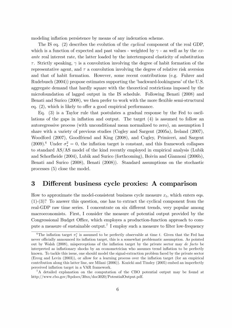
How to approximate the model-consistent business cycle measure xt, which enters eqs.(1)-(3)? To answer this question, one has to extract the cyclical component from thereal-GDP raw time series. I concentrate on six di¤erent trends, very popular amongmacroeconomists. First, I consider the measure of potential output provided by theCongressional Budget O¢ ce, which employes a production-function approach to com-pute a measure of sustainable output.7 I employ such a measure to �lter low-frequency

6The in�ation target ��t is assumed to be perfectly observable at time t. Given that the Fed hasnever o¢ cially announced its in�ation target, this is a somewhat problematic assumption. As pointedout by Walsh (2008), misperceptions of the in�ation target by the private sector may de facto beinterpreted as in�ationary shocks by an econometrician who assumes trend in�ation to be perfectlyknown. To tackle this issue, one should model the signal-extraction problem faced by the private sector(Erceg and Levin (2003)), or allow for a learning process over the in�ation target (for an empiricalcontribution along this latter line, see Milani (2006)). Kozicki and Tinsley (2005) embed an imperfectlyperceived in�ation target in a VAR framework.

7A detailed explanation on the computation of the CBO potential output may be found athttp://www.cbo.gov/ftpdocs/30xx/doc3020/PotentialOutput.pdf.

6

movements of the real GDP out of the raw series, and I label this empirical proxy �CBO�.The second transformation is obtained by applying the popular Hodrick-Prescott (�HP�)�lter with standard weight 1,600. The third transformation is a classical trend-cycledecomposition obtained by �tting a constant and a linear trend to the raw series with-out allowing for any break in the sample, and taking the residuals as indicator of thebusiness cycle (�LIN�). By contrast, the fourth manipulation (�LBR�) �ts a piecewiselinear trend with a break in 1980:III in both the constant and the slope parameter.Another proxy I consider is constructed by applying the Baxter and King (1994) band-pass �lter (�BP�) to the log-real GDP so to extract cycles within the [8,32] quartersperiodicity (with 12 quarters left as leads/lags). Finally, I take the growth rate ofthe raw series (�FD�) as an indicator of GDP�s cyclical component, a choice that reliesupon the random walk with drift as a model for the real GDP trend. I perform allthese transformations by considering the sample 1954:III-2008:II, a span longer thanthe one I employ to estimate the NKBC model. This choice�s aim is that of tacklinginitial-condition issues concerning some of the �lters at hand.The �lters I consider are very widely employed in the macroeconomic literature.8 Im-

portantly, they are heterogeneous along di¤erent dimensions. Some �lters compute thenon-cyclical component with quasi-deterministic procedures (LIN, LBR), some assumeit is stochastic but very smooth (HP, BK), some very volatile (FD). Some proceduresemploy univariate information, others a larger set (CBO). Some are one-sided (FD),others two-sided (LIN, LBR, HP, BP). As regards low-frequency distortions, some arelikely to overestimate the contribution of the low frequency variability on the businesscycle (LIN, LBR), others underestimate it or possibly estimate it fairly precisely (BP).Figure 1 - left column displays the business cycle empirical proxies obtained with

the six �lters described above. One may spot similarities and di¤erences across theseproxies. Some comments are in order. First, �eyeball econometrics�suggests a positivecorrelation across proxies, which is also con�rmed by the �gures reported in Table 1.However, such correlation varies - in some cases, dramatically - when moving from a pairto another. The highest correlation - 0.94 - regards the pair (HP,BP), while the lowest -0.10 - involve (LIN,FD). In general, FD is poorly correlated with the rest of the businesscycle indicators. This is due to the somewhat erratic behavior displayed by this proxy,which also signals shorter cycles with respect to alternatives. The di¤erent proxiesunder investigation display a relevant amount of heterogeneity also in terms of businesscycle dating. Taking the NBER recessions (identi�ed by the grey bars in Figure 1) asreference, one may observe that CBO and HP perform reasonably well. By contrast,LIN just misses to capture the 1969:IV-1970:IV, 1973:IV-1975:I, and 1980:I-1980:III

8Of course, the list of �lters one may think of is much larger. Canova (1998), Canova (2007)(Chapter 3), Cogley (2008), and Proietti (forthcoming) consider a set of alternative �lters and discussthe pros and cons of di¤erent �ltering strategies at length.

7

recessions, which are considered as simple slowdowns - i.e. realizations of decreasingbut positive output gaps, while LBR shows a somewhat better ability in matching suchrecessions. Still sticking to the dating issue, FD shows the worst performance, with noclear indication of any particular recession, with the exception of the early 1980s one,indeed caught by all the proxies at hand. The magnitude of booms and busts is clearly�lter-dependent, with some �lters - e.g. LIN - possibly magnifying the deviations withrespect to �potential�output and others - e.g. FD - dampening them. Table 1 con�rmsthe high volatility in terms of estimated variance of the cyclical component of output.The highest �gure - 11.61 - is associated to the LIN �ltered proxy, whose variance ismuch larger than those of the widely employed CBO and HP- respectively 5.76 and2.90 - and de�nitely greater than the one of the real GDP growth rate, with the ratiobetween the two being close to sixteen! Interestingly, when allowing for a break in thetrend coe¢ cients, the variance of the linearly detrended business cycle proxy drops ofabout 40%, so getting much closer to those of HP and CBO. The FD indicator returnsthe lowest variance - 0.73, and the BP �lter induces the second lowest variance - 1.68.Such heterogeneity is also re�ected by the AutoCorrelation Functions depicted in

Figure 1 - middle panel. In terms of autocovariance structure, a very di¤erent storyis told by �lters like HP and BP when contrasted to FD, with the latter showing avery quick drop of persistence after a few lags and a mild oscillatory behavior aroundzero thereafter, while the former display higher persistence and wide oscillations overthe twenty-�ve lags considered. Accounting for the break in the linear trend induces aswitch of the sign for most of the autocovariances of LBR with respect to LIN. Table1-last row, however, suggests that the estimated persistence of the business cycle isvery high, with the exception of the FD manipulation. Figure 1 - right panel depictsthe log-Spectra of the proxies at hand. It is easy to spot signi�cant errors in termsof identi�cation of the frequencies of interest. Ideally, business cycle indicators shouldretain frequencies corresponding to the range 8 to 32 quarters (identi�ed by the verticalblack dotted bars in the normalized frequency domain). Notably, our proxies tend toattribute an excessive power to low-frequencies, but the error is clearly heterogeneousacross �lters, with the BP �lter performing (by construction) better than all other�lters, the HP �lter o¤ering an �intermediate�performance, and others - among whichthe CBO �lter - overemphasizing the relevance of low-frequency �uctuations for thebusiness cycle.9 In general, problems of leakage (loss of power at the edges of thebusiness cycle frequency band) and compression (increase of power in the middle ofthe band) are pervasive, a result already pointed out by, among others, Canova (1998),Canova (2007), Chapter 3), Canova (2009), Proietti (forthcoming), and Canova andFerroni (2009).

9The log-Spectra is computed with the �pwelch�Matlab function. A Bartlett window kernel of size21 was employed to smooth the periodogram and obtain a consistent estimation of the spectra.

8

In short, commonly applied �lters tend to comove but are very heterogeneous acrosssome dimensions - dating, magnitude, average length, and persistence of the businesscycle. These di¤erences are key. One the one hand, they may trigger a ��lter-induced�heterogeneity in results, the quanti�cation of which is ultimately what this paper isafter. But this heterogeneity is also a source of relevant information. As stressed byCanova and Ferroni (2009), heterogenous business cycle representations in the frequen-cies of interest enable the econometrician to optimally extract the relevant informationembedded by each �contaminated proxy�in the estimation phase. Which are the impli-cations of using di¤erent �lters in terms of model estimation? The next Sections tacklesthis issue.

4 Model estimation with multiple �lters

To appreciate to what extent �ltering may be econometrically relevant, I �rst estimatethe NKBCmodel (1)-(5) by using all the proxies scrutinized in the previous Section one-by-one. This exercise will provide information on the �lter-induced heterogeneity in theestimated objects of interest. Then, I perform estimations by considering the di¤erentproxies jointly. Canova and Ferroni (2009) point out that this procedure has threemain advantages. First, it does not require the researcher to take a strong a-prioristand on how to model the trend and the shocks driving it. Given the uncertaintysurrounding the evolution of factors like technology and preferences, the fact of beingable to remain agnostic on which �lter to use is likely to work towards the reduction ofbiases due to trend misspeci�cation. Second, this methodology allows to employ cyclicaldata computed with �lters having very di¤erent features, e.g. one vs. two-sided �lters,univariate vs. multivariate, deterministic vs. stochastic, and so on, so making parameterestimates more robust to �lter misspeci�cation. Third, errors in the attribution of thebusiness cycle frequencies are proxy-speci�c. If such errors display a somewhat commonpattern across proxies, the joint employment of di¤erent empirical indicators of thebusiness cycle should reduce small sample biases in parameters estimates. If such errorsare more idiosyncratic, this estimation procedure should wash them out so deliveringmore precise estimates. Canova and Ferroni�s (2009) Monte Carlo exercises con�rm thatthe joint employment of multiple �lters reduce the biases of the estimated parametersas well as impulse response functions.To estimate the model (1)-(5), I therefore set up the following encompassing mea-

surement equation:

9

26666664

FFRATEtINFLGDPt264 ex1t

...exNt375

[Nx1]

37777775 =26666664

R�264 ex1...exN375

[Nx1]

37777775+26666664

�1 00 1

�0

[2xN ]

0[Nx2]

264 �1 ::: 0

0. . . 0

0 ::: �N

375[NxN ]

37777775

26666664

Rt�t264 xt...xt

375[Nx1]

37777775+26666664

00264 u1t...uNt

375[Nx1]

37777775 ;(6)

where FFRATEt is the quarterly federal funds rate at time t, INFLGDPt is thequarterly GDP de�ator in�ation, ext = [ex1t; :::; exNt]0 is the (Nx1) vector of empiricalproxies of the business cycle computed withN di¤erent approximations of the trend, ex =[ex1; :::; exN ]0 is a (Nx1) vector of proxy-idiosyncratic constants to demean the �lters, � is a(NxN) diagonal matrix of �loadings�relating the model consistent cyclical component xtto the N empirical proxies ext, and ut = [u1t; :::; uNt]0 � i:i:d:(0Nx1; diag(�2u1; :::; �2uN)) isa (Nx1) vector of serially and mutually uncorrelated �lter-speci�c measurement errors.If a given �ltered measure exnt; n 2 f1; :::; Ng represented exactly the model consistentbusiness cycle, one should expect the slope �n to be statistically equal to one, and thevolatility of the measurement error �2un to be close to zero. Then, the slope parametersindicate the weights assigned by the data to the �signals�delivered by a given �lter asregards the cyclical component of real GDP when contrasted with the model-consistentbusiness cycle indicator. The associated measurement errors indicate the uncertaintysurrounding such signals. When implementing the multiple �lter strategy, I normalize�CBO = 1, and I interpret the remaining �s as relative loadings with respect to the �rstone. By contrast, when estimating the model with a single proxy, the measurementequation (6) features N = 1, ext = [exnt]0; ut = [unt]

0, and the restriction � = [�n]0 = 1is imposed. A measurement error to the business cycle equation in (6) is allowed alsowhen a single proxy is employed.Notice that pre-�ltering is applied neither to in�ation nor to the federal funds rate.

In the model at hand, in�ation is �ltered by the in�ation target process (4), whichallows to construct a model consistent in�ation gap measure, i.e. �t � ��t . As for thefederal funds rate, the absence of pre-�ltering enables a consistent comparison of theresults of this paper to those o¤ered by previous contributions, which typically do notperform any manipulation on the raw nominal rate (for further discussions, see Section5.4).

Bayesian estimationI perform econometric estimations by relying upon Bayesian techniques, widely em-

ployed in the applied macroeconomic literature (see An and Schorfheide (2007) andFernandez-Villaverde (2009) for detailed reviews, and Canova and Sala (2009) for a dis-cussion of the pros and cons of this methodology vs. alternatives). I then need to set

10

priors so to augment the likelihood of the model with some a-priori knowledge. Follow-ing Cogley, Primiceri, and Sargent (2009), I set the autoregressive parameter �� of thein�ation target process (4) to 0:995 to capture low-frequency movements in in�ation.Consequently, the zero-frequency of the in�ation process is almost entirely explainedby shocks to trend in�ation. This does not necessarily imply, however, that shocks totrend in�ation are, by construction, the main driver of the conditional volatility of in-�ation. By contrast, the standard monetary policy shock is assumed to be white-noise.This di¤erence enhances the identi�cation of the two monetary policy shocks. As it iscustomary in the literature, I calibrate the discount factor � to 0.99.The remaining priors - reported in Table 2 - are fairly standard, and roughly in line

with Benati and Surico (2008), Benati (2008), Benati (2009), and Cogley, Primiceri,and Sargent (2009) as regards the parameters in common between their models and theone under investigation. In particular, I aim to be relatively uninformative as far as thepersistence parameters are concerned, and I allow the domain of the volatilities of themodel to be wide enough to let the data free to indicate the relative impact of the variousshocks on the U.S. economic system. Finally, I assume the loadings of the empiricalproxies to be independently distributed as �i � N(1; 0:5). Measurement errors are alsoassumed to be independently distributed and follow uit � Inverse Gamma(0:25; 2).10I use as raw data the U.S. GDP de�ator, the log-real GDP, and the federal funds

rate (average of monthly observations), all downloaded from the website of the FederalReserve System.11 In line with e.g. Cogley, Primiceri, and Sargent (2009), I considerthe following two subsamples: 1960:I-1979:II, which corresponds to the �Great In�ation�period before the appointment of Paul Volcker as Fed�s chairman, and 1982:IV-2008:II,which corresponds to the post-�Volcker experiment�/�Great Moderation� sample. Allseries (�ltered outputs, in�ation, and the policy rate) are demeaned prior to estimation.Consequently, I set R, �, and the vector ex to zero.1210The �gures reported in brackets refer to the mean and standard deviation of the distributions of

interest.11URL: http://research.stlouisfed.org/fred2/ .12To perform Bayesian estimation I employed Dynare 4.0, a set of algorithms developed by Michel

Juillard and collaborators and freely available at http://www.cepremap.cnrs.fr/dynare/. The mode ofeach parameter�s posterior distribution was computed by using the �csminwel�algorithm elaboratedby Chris Sims. A check of the posterior mode, performed by plotting the posterior density for valuesaround the computed mode for each estimated parameter in turn, con�rmed the goodness of theoptimizations. I employed such modes to inizialize the random walk Metropolis-Hastings algorithm tosimulate the posterior distributions. The inverse of the Hessian of the posterior distribution evaluatedat the posterior mode was used to de�ne the variance-covariance matrix of the chain. The initial VCVmatrix of the forecast errors in the Kalman �lter was set to be equal to the unconditional variance ofthe state variables. I used the steady-state of the model to initialize the state vector in the Kalman�lter. I simulated two chains of 200,000 draws each, and discarded the �rst 75% as burn-in. To scalethe variance-covariance matrix of the random walk chain I used a factor so to achieve an acceptancerate belonging to the [23%,40%] range. To assess the stationarity of the chains, I considered theconvergence checks proposed by Brooks and Gelman (1998). I conditioned the estimation of the model

11

5 Empirical results

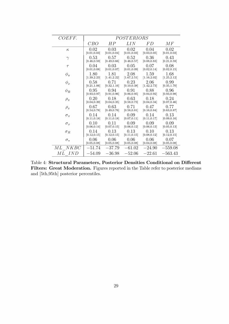
Canova and Ferroni (2009) show that the MF approach is superior to single-�lter al-ternatives in presence of su¢ cient idiosyncratic information in the set of contaminatedproxies of the business cycle employed in the estimation. The loadings of such proxies(posterior median values) range from 0.85 (LBR) to 4.34 (FD) in the Great In�ationsample, and from 0.80 (LBR) to 4.88 (FD) in the more recent period, con�rming thepresence of heterogeneous information provided by the di¤erent �lters. I then take theestimates obtained with MF as a reference when conducting comparisons across �lters.Tables 3 and 4 collect �gures concerning the posterior distributions of some rep-

resentative models. To have a complete screening of the results, Figure 2 plots thedensities of all estimated models across the two subsamples. All the posterior mediansappear to be economically sensible. Indeed, one may spot striking di¤erences across�lter-induced estimates and in contrast to the MF�s median. Remarkable �lter-speci�cuncertainty surrounds the intertemporal elasticity of substitution, the extent to whichagents are forward-looking in the IS curve, the long-run reaction of the Fed to in�ationand output gap �uctuations, the persistence of the shocks, and their volatilities (withthe exception of the volatility of the trend in�ation shock, which appears to be fairlystable across �lters). Given that counterfactuals are typically run by relying on suchdensities or, often, by conditioning on their means/medians, one may very well wonderhow reliable the conclusions of such exercises should be considered in the light of thejust documented proxy-induced uncertainty.Interestingly, there are also similarities across the estimated models. The long-run

reaction to in�ation gap oscillations increase when moving to the Great Moderationsubsample, even if not necessarily so in a statistical sense. This �nding is in line withCogley, Primiceri, and Sargent (2009), and resembles the one proposed by Clarida, Gali,and Gertler (2000), Lubik and Schorfheide (2004), and Boivin and Giannoni (2006b).Notice that, as in Cogley, Primiceri, and Sargent (2009), the di¤erence between thesystematic reactions to in�ation gap �uctuations in the two subsamples is not large.This might be due to the imposition on equilibrium uniqueness in the estimation phase.13

Another possible explanation could be the di¤erent object at hand, i.e. the in�ation

to the unique-solution parameter region.13The debate on the evidence in favor of an indeterminate equilibrium in the pre-Volcker subsample

is very lively. On the one hand, Clarida, Gali, and Gertler (2000), Lubik and Schorfheide (2004), andBoivin and Giannoni (2006b) lends support to indeterminacy. Castelnuovo and Surico (2009) show thatindeterminacy may o¤er a rationale for the price puzzle typically found when estimating the e¤ects ofa monetary policy shocks with VAR models. Surico (2006) discusses the perils coming from mergingtwo subsamples characterized by di¤erent equilibria when conducting empirical exercises on NKPCs.By contrast, Sims and Zha (2006), Justiniano and Primiceri (2008b), Cogley, Primiceri, and Sargent(2009), and Canova and Gambetti (2009) cast doubs on multiple equilibria as a relevant feature todescribe the economic situation in the 1960s and 1970s.

12

gap in this study vs. raw in�ation in Clarida, Gali, and Gertler (2000), Lubik andSchorfheide (2004), Boivin and Giannoni (2006b). With a model similar to the oneemployed in this paper, Castelnuovo (2009) obtains �more conventional�estimates forthe Taylor parameters under the assumption of a constant in�ation target.14

A robust result I obtain is the generalized reduction of the volatilities of the struc-tural shocks in the second subsample, a �nding that captures in �rst approximation theevidence put forward by Justiniano and Primiceri (2008b) with a framework allowingfor time-varying conditional volatilities. Notably, the variance of the in�ation targetshock is lower in the second subsample. This �nding, which I share with Stock andWatson (2007) and Cogley, Primiceri, and Sargent (2009), candidates the reduction intrend in�ation volatility as one of the possible drivers of the Great Moderation.15

5.1 Comparison with the standard price indexation model

It is worth scrutinizing how the model I focus on performs with respect to the standardprice-indexation model displaying no time-varying in�ation target. To do so, I considera version of the model featuring the following version of the NKPC and Taylor rule:

�t =�

1 + ��Et�t+1 +

�

1 + ���t�1 + �xt + "

�t ; (7)

Rt = (1� �R)(���t + �xxt) + �RRt�1 + �Rt : (8)

Eq. (7) displays the parameter �, which identi�es non-reoptimizing �rms�indexationto past in�ation. Eq. (8) is a standard Taylor rule postulating a systematic reactionto in�ation oscillations by the Fed. In a constant-in�ation target (demeaned) world,in�ation and in�ation gap are coincident objects. As already mentioned, in�ation targetshocks have been found to be empirically relevant as drivers of the post-WWII U.S.in�ation (Cogley and Sargent (2005a), Ireland (2007), Castelnuovo, Greco, and Raggi(2008), and Cogley, Primiceri, and Sargent (2009)). If this is the case, a standard Taylorrule with a constant in�ation target is likely to o¤er a misspeci�ed representation ofthe U.S. monetary policy conduct.To engage in a formal comparison between my benchmark (NKBC) model (1)-(5)

model and the alternative indexation (IND) framework, I estimate also the latter (com-posed by eqs. (2), (5), (7), (8)) with di¤erent proxies of the business cycle. In sodoing, I follow Benati (2008) and model the in�ation shifter "�t as a white noise, so

14Further investigations on this issue are conducted, in the context of regime-switching Taylor rulemodels, by Castelnuovo, Greco, and Raggi (2008).15The drop of the trend in�ation volatility shock may at a �rst glance appear to be negligible.

However, one must bear in mind that the autoregressive root �� = 0:995, then a drop of " in thevolatility of the trend in�ation shock translates into a reduction of about 1

1�0:9952 � 100" in theunconditional volatility of trend in�ation.

13

giving the indexation parameter � the highest chance of grasping the U.S. in�ationpersistence. Tables 3 and 4 (ast two rows) collect the (log) Marginal Likelihoods ofthe NKBC and IND models.16 Some comments are in order. First, the NKBC modelwith trend in�ation is clearly preferred in four of the �ve comparisons reported in Ta-ble 3 - Great In�ation. Indeed, price indexation acts as an imperfect �substitute�ofthe time-varying in�ation target. This result squares up with those put forward byIreland (2007) and Cogley and Sbordone (2008), which favor a new-Keynesian Phillipscurve formulation with trend in�ation and no indexation when contrasted to a modelendowed with price indexation. The only exception is represented by the FD scenario,which supports instead the IND model. This is possibly due to the low volatility ofthe FD cyclical component, which may perhaps capture some of the low frequencies inin�ation otherwise caught by trend in�ation. Notably, the posterior odd clearly favorsthe NKBC model when multiple �lters MF are considered.A somewhat less de�ned picture arises when considering the Great Moderation sub-

sample. In this latter case, three models out of �ve - HP, LIN, FD - support the priceindexation model. This is perhaps not too surprising. The Great Moderation periodis characterized by low and fairly stable in�ation, and the role of trend in�ation forthe dynamics of raw in�ation is possibly less relevant. However, the CBO �lter and,importantly, the MF panel of �lters support the NKBC model with time-varying trendin�ation. This latter result casts doubts on the ability of a single �lter to identify theshocks driving the U.S. macroeconomic processes. Overall, when considering both sub-samples, the trend in�ation model appears to be preferrable. Moreover, it is naturallysuited to investigate the role played by trend in�ation shocks in shaping the post-WWIIU.S. macroeconomic environment. Then, in the reminder of the paper I will exclusivelyfocus on such a model.17

5.2 Impulse response functions

Figure 3 displays the impulse response functions to the two monetary policy shocksa¤ecting the system, the �traditional�shock to the nominal interest rate in the Taylorrule (3) and the shock to the trend in�ation process (4). In all cases, the reactionshave the expected sign. A monetary policy tightening induces an increase in the policy

16Preliminary attempts to estimate the IND model with the priors reported in Table 2 failed due tothe di¢ culty of computing posterior modes. I veri�ed that a smooth convergence was instead possibleby manipulating the prior mean of the slope of the NKPC. The estimations of the IND model are thenconditional on � � Gamma(0:035; 0:01).17Notice that, given the di¤erence in terms of �observables�, I cannot perform Marginal-Likelihood

based comparisons across �lters. This is due to the procedure at hand, which implies a �lter-speci�cdataset. Di¤erently, Ferroni (2009) and Canova (2009) �lter raw data and estimate the DSGE cyclicalmodel jointly, i.e. in a single-step fashion. This strategy enables them to compare the empiricalperformance of di¤erent �lters.

14

rate as well as in the real interest rate, a decrease in the output gap, and a demand-driven de�ation. A positive in�ation target shock triggers a take-o¤ in in�ation andcalls for a monetary policy tightening. Given that policymakers react with gradualism,the real interest rate takes negative values in the short run, which leads to a temporaryexpansion. These reactions are qualitatively in line with those put forward by Ireland(2007) and Cogley, Primiceri, and Sargent (2009).However, while the dynamics of the system are qualitatively clear, Figure 3 also

shows that the situation is quite shaded when seen from the quantitative angle. Infact, the business cycle reaction to both shocks in both subsamples is extremely het-erogeneous.18 To �x ideas on this concept, I compute the percentage deviations of eachestimated reaction with respect to the MF �lter. Table 5 collects the �gures regardingthe 4 and 8-quarter ahead percentage deviations. The estimated di¤erences across �ltersand between each �lter and the MF representation are striking. As regards the standardpolicy shock, �gures related to the 4-quarter horizon range from the zero deviation sug-gested by the CBO �lter to the 50% of FD, with HP and LIN associated to a deviationof about 30% under the Great In�ation sample. Interestingly, when accounting for thebreak, the linear trend lines up (in terms of deviations) to the CBO trend. Figures aresomewhat magni�ed under the Great Moderation sample, with FD�s deviation reading75%. 8-quarter ahead predictions suggest larger �gures for all the �lters but BP underthe Great Moderation.Filter-uncertaintly clearly a¤ects also the estimated reaction of in�ation to a stan-

dard monetary policy shock. Again, CBO suggests milder deviations when contrastedto HP and LIN, and LBR somewhat dampens the e¤ects induced by LIN. Notably,the widely employed HP �lter is associated to a percentage deviation of about 40%(8-quarter ahead), a very large departure indeed. The growth rate, once more, turnsout to be the �lter deviating the most with respect to the MF �weighted average�, with�gures over 80%.Also in�ation target shocks trigger quantitatively very di¤erent business cycle re-

sponses. Under Great In�ation, the 4-quarter ahead business cycle reaction to a trendin�ation shock inducing a 1% on impact hike in the in�ation rate reads 17%, 34%,and 44% when - respectively - HP, LIN, and FD �lters are considered under the GreatIn�ation, and even larger under the Great Moderation, with FD�s departures peaking75% in the 8-quarter ahead scenario. Interestingly, in�ation reactions turn out to bemuch more homogeneous, with the highest deviation being 5.78% (8-quarter ahead).This might be due to the role played by the direct impact exerted by in�ation targetshocks on the in�ation rate via the NKPC (1).

18Credible sets (con�dence bands) are intentionally not displayed. The point here is that of assessingthe heterogeneity due to the �ltering choice, and not the sample uncertainty surrounding objects likeimpulse responses or forecast error variance decompositions.

15

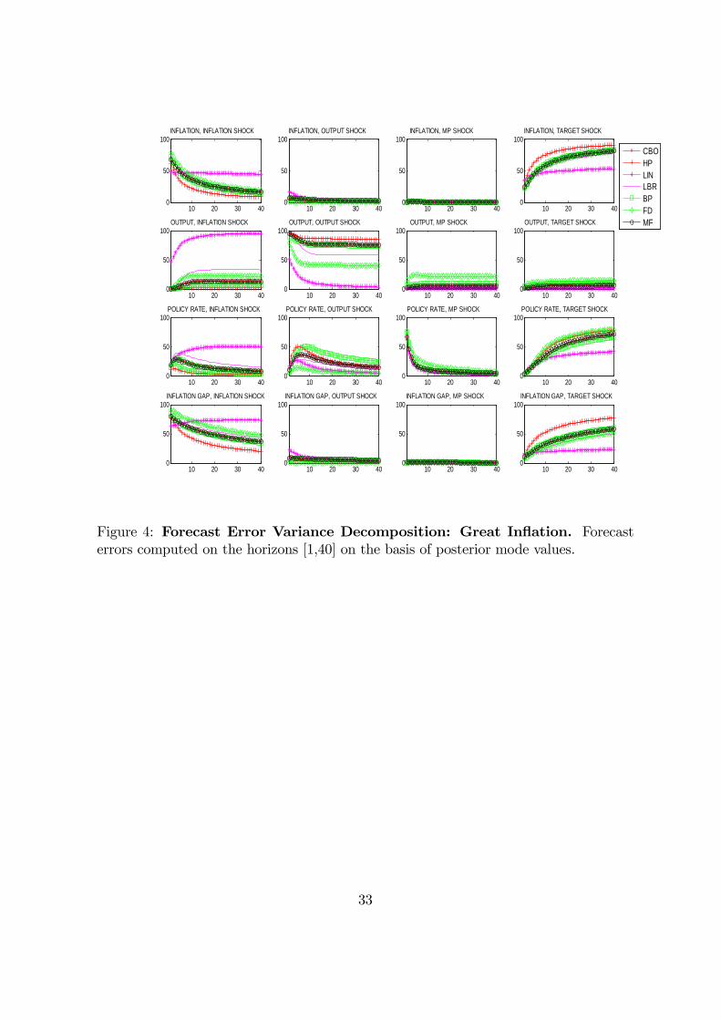
5.3 Forecast error variance decomposition

To gain some information on the role that �ltering may play for the identi�cation of theshocks driving the U.S. macroeconomic dynamics, I estimate the forecast error variancedecomposition at di¤erent horizons.19 Figures 4 and 5 show this information for the twosubsamples of interest. Once again, �ltering matters. A few striking examples supportthis statement. If one wants to assess the contribution that �in�ation� shocks havehad on output dynamics at - say - a forty-quarter horizon, she has to face the ratherpuzzling situation of choosing between the 100% contribution suggested by LIN versusthe virtually 0% contribution proposed by the HP �lter (both during the Great In�ationand under Great Moderation). Filter-induced heterogeneity is visually detectable inboth subsamples when looking at in�ation in reaction to monetary policy shocks, outputto output and in�ation shocks, the policy rate and the in�ation gap to basically allshocks. The contribution of the in�ation shock to the policy rate tells a story similarto that of the contribution of the very same shock to the business cycle. The standardmonetary policy shock turns out to be relevant for the dynamics of the policy rate andfor the business cycle, with the latter being mainly a¤ected under the Great Moderation.By contrast, the direct impact of the traditional policy shock appears to play a negligiblerole for in�ation and the in�ation gap. Also the contribution to in�ation target shocksto in�ation, the in�ation gap, and the policy rate is subject to a considerable amountof uncertainty in absolute terms, but tends to be relatively large and increasing oversubsamples. By contrast, the impact of trend in�ation shocks on the business cycleappears to be negligible in both subsamples.Table 6 collects percentage deviations of the �lter-speci�c contributions of the two

monetary policy shocks on in�ation and output with respect to the one associated toMF. Some common patterns with the previously analyzed �lter-speci�c impulse re-sponse function arise. In fact, one may notice that HP, LIN, and FD suggest decom-positions that are percentually very di¤erent with respect to the one proposed by MF,both when looking at 16-quarter ahead and when going for the �long run�- 40-quarterahead. Percentage deviations are relatively less important in the case of in�ation underthe Great In�ation period for most of the �lters but HP and LIN. Again, accountingfor the break in the linear trend lines remarkably dampens the departures from MF,which are anyhow still present. Interestingly, while the standard monetary policy shockis subject to a very large amount of �lter-induced uncertainty, that surrounding thecontribution of trend in�ation shocks for the in�ation process is much lower. Indeed,the highest departure concerning this latter shock is that of LIN under the Great Mod-eration - about 35%. Much larger �gures are those associated to the reactions to astandard unexpected policy rate hike, a chief example being the contribution of the

19I thank Marco Ratto for kindly providing me with the �vardec.m�code to compute the forecasterror variance decomposition at di¤erent horizons.

16

standard monetary policy shock for output under the Great In�ation sample - 340%!This suggests that the large contribution assigned to trend in�ation shocks by all �ltersas regards in�ation is a very robust fact. This �nding lines up with recent research-Ireland (2007), Cogley, Primiceri, and Sargent (2009) pointing towards trend in�ationshocks as the main in�ation driver of the post-WWII U.S. period. This is relevant,because it lends support to studies aiming at understanding the reasons behind trendin�ation, one of the possible reasons being learning of the structure of the economy bythe U.S. monetary policy authorities (Cogley and Sargent (2005b), Primiceri (2006),Sargent, Williams, and Zha (2006), and Carboni and Ellison (2009)).Wrapping up, the evidence presented above clearly points towards a marked �lter-

induced heterogeneity in the posterior densities and, consequently, dynamic responsesand variance decompositions when a standard, �operational� business cycle model istaken to the data.

5.4 Robustness checks

I ran some checks to verify the solidity of the previously discussed empirical �ndings.In particular,

� I re-estimated the model with multiple �lters by dropping the FD �lter, whichappears to be an outlier when contrasted to the other �lters at hand. Indeed,the presence of the FD �lter enhances the heterogeneity of the �lters across thefrequencies of interest. On top of that, the information content of the FD businesscycle proxy is weighted �endogenously�via the estimated �FD per each subsample,and its precision is assessed via its period-speci�c measurement error variance.However, to be sure that such particular �lter is not driving the results in anyimportant manner, I undertook the estimation of the model with the remaining�ve �lters and re-plotted IRFs and FEVDs. The results presented above turnsout to be robust to this manipulation;

� I re-estimated the model by considering the cyclical representation also of in�ationand the policy rate on top of that of real GDP. E.g., the model �HP�has beenestimated with HP �ltered log-real GDP, HP �ltered GDP de�ator in�ation, andthe HP �ltered federal funds rate (the same holds for the remaining �lters).20

The main conclusion of this paper, i.e. the pervasive heterogeneity induced bydi¤erent �lterings as regards IRFs and FEVDs, is una¤ected. Not surprisingly,the impact of trend in�ation shocks turns out to be dampened for most of the

20The LBR �lter was not considered due to multicollinearity issues in the MF application. Wedid not �lter in�ation and the policy rate in the CBO case, which is constructed on the basis of thepotential output as computed by the Congressional Budget O¢ ce.

17

�lters. However, one should take this last result with care. Indeed, the structuralmodel (1)-(5) already displays a �lter for raw in�ation (and, indirectly, the policyrate), which is the in�ation target process. Then, the reduction in the importanceof in�ation target shocks is likely to be driven by �over-detrending�;

� In the baseline battery of estimations I employed demeaned data and set R, �,and the vector ex to zero. In fact, as pointed out by Canova and Ferroni (2009),estimating the constants of the model may be informative on the �level biases�associated to each �lter. As a �quality-check�, I re-estimated the MF models byallowing for independently distributed �lter-speci�c constants exn � N(0; 0:5),n 2 f1; :::; Ng. A large departure from the zero-value of a given �lter-speci�cconstant would cast doubts on that �lter�s ability to correctly identify the meanof the business cycle process. However, the vector ex is estimated to be very closeto zero, and with small standard errors, a result suggesting the absence of levelbiases.

These results, not documented here for the sake of brevity, are available upon re-quest.

6 Contacts with the literature

This paper is closely related to some recent contributions regarding �ltering and the es-timation of DSGE models on the one hand, and the role played by trend in�ation shockson the other. As previously pointed out, Canova and Ferroni (2009) propose a method-ology to jointly deal with di¤erent contaminated proxies of the cyclical component ofthe variables of interest when taking the model to the data. They perform a MonteCarlo analysis to study the properties of their proposal, and show that the joint em-ployment of di¤erent �lters returns estimated parameters and impulse responses muchmore consistent than those obtained with a standard single-�lter approach. Then, theytake a new-Keynesian business cycle model of the business cycle to the data, and showthat money enters signi�cantly both the in�ation schedule and the aggregate demandequation, a �nding overturning previous results. The Fed is also shown to have system-atically reacted to oscillations in the growth rate of money. While employing Canovaand Ferroni�s (2009) methodology, my paper focuses on di¤erent objects, i.e. ultimatelythe �lter-induced heterogeneity concerning the conditional reaction of in�ation and out-put to two di¤erent monetary policy shocks and the contribution of identi�ed structuralshocks to the U.S. macroeconomic volatility.Related papers are Ferroni (2009) and Canova (2009). Ferroni (2009) contrasts the

standard ��rst �lter, then estimate�two-stage approach with a novel �jointly �lter andestimate�one-step strategy. The novelty hinges upon the joint estimation of trend and

18

structural parameters. Importantly, this strategy allows a researcher to exploit thecross-equation restrictions of the DSGE model when performing the trend-cycle de-composition, to compare the descriptive ability of di¤erent �lters, and to employ theresulting information to construct robust estimates via Bayesian averaging. Ferroni�s(2008) �trend agnostic�methodology turns out to be more consistent than alternativesalso in case of model misspeci�cation. He also estimates a standard AD/AS model withU.S. data and show that di¤erent �lters may indeed induce di¤erent estimates of theparameters/moments of interest. Canova (2009) also proposes a �single step�method-ology that allows for a �exible link between un�ltered raw data and the theoreticalmodel at hand, and in which cyclical and non-cyclical components are allowed to havepower in all the frequencies of the spectrum. Simulations performed by the author showthat standard data transformations induce distortions in structural estimates and policyconclusions that are drastically reduced when applying his methodology. With respectto Ferroni (2009) and Canova (2009), I undertake a more conventional �two-stage strat-egy�to highlight the consequences of detrending in the context of a modern monetarypolicy model of the business cycle that embeds, among others, trend in�ation shocks,i.e. possibly one of the main drivers of the great moderation in in�ation (Cogley, Prim-iceri, and Sargent (2009)). Moreover, I jointly consider a variety of di¤erently �lteredbusiness cycle representations and let the data speak about their relative weights.Cogley (2001) suggests to estimate the model with GMM techniques before solving

the Euler equations for rational expectations, so to avoid to specify the driving processesat the estimation stage. Instead, I stick to the ��rst solve, then estimate� sequencetypically called for by likelihood-based estimation techniques, also to overcome theweak-instrument problem often arising when employing GMM techniques (e.g. Fuhrerand Rudebusch (2004)).In terms of empirical application, a recent contribution by Delle Chiaie (2009) con-

trasts the estimates of a medium-scale DSGE model for the Euro area conditional onthe employment of linear vs. HP �lter. Dramatic di¤erences in terms of posterior densi-ties and impulse response functions arise. While being quite correlated to Delle Chiaie�s(2009) research idea, my paper employes a larger variety of �lters, and it combines themaccording to the proposal by Canova and Ferroni (2009).From a more exquisitely economic standpoint, my contribution intersects those con-

cerned with the modeling of the U.S. in�ation and output. One of the main features ofin�ation is its persistence, which has often been modeled via somewhat ad hoc indexa-tion mechanisms. Going against this tendency, Cogley and Sbordone (2008) and Benati(2009) show that, once trend in�ation is embedded in the new-Keynesian Phillips curve,price indexation is statistically not signi�cant. The remarkable evidence supporting thehypothesis of a time-varying in�ation target pursued by the Fed (Cogley and Sargent(2001), Cogley and Sargent (2005a), Ireland (2007), Stock and Watson (2007), Cog-

19

ley, Primiceri, and Sargent (2009), Castelnuovo, Greco, and Raggi (2008), Castelnuovo(2009), and the two previously mentioned papers) motivates my choice of working witha model in which trend in�ation is allowed to play an active role in shaping the U.S.in�ation process.

7 Conclusions

This paper has estimated an �operational�new-Keynesian model of the business cycle(NKBC) with single and, following Canova and Ferroni (2009), multiple �lters to assessthe role that �ltering choices may play as regards objects of interest such as posteriordensities, impulse response functions, and forecast-error variance decompositions.My �ndings read as follows. Di¤erent proxies of the �output gap�, widely employed

in the applied macroeconomic literature, are remarkably heterogeneous in terms ofturning points, volatility, and persistence, and share low-power when it comes to isolatebusiness cycle frequencies. When employed to estimate the NKBC model I consider, Ifound that the �lter-induced uncertainty surrounding the values of some key parameters- slope of the Phillips curve, degree of intertemporal elasticity of substitution, Taylorrule parameters, persistence and volatility of the structural shocks - is substantial. Thisuncertainty a¤ects also impulse response functions to a standard monetary policy shockand variance decompositions. These results, conceptually in line with those presentedin Canova (2009), Ferroni (2009), and Canova and Ferroni (2009), raise the issue of therobustness of the identi�cation of the drivers of the U.S. great moderation to di¤erent�ltering strategies.This uncertainty notwithstanding, a very solid �nding stands out. Shocks to trend

in�ation turn out to be the main driver of the post-WWII U.S. in�ation. This resultsquares up with recent �ndings by Ireland (2007) and Cogley, Primiceri, and Sargent(2009), and it lends support to research investigating the evolution of the low-frequencycomponent of the post-WWII U.S. in�ation rate. A possible explanation is learning,i.e. imperfect knowledge of the economic structure and the formation of the beliefs onthe evolution of the perceived in�ation-output volatility trade-o¤ by the Fed. Cogleyand Sargent (2005b), Primiceri (2006), Sargent, Williams, and Zha (2006), and Carboniand Ellison (2009) have proposed interesting investigations along this dimension.The employment of a rich set of cyclical macroeconomic measures is a promising

avenue to perform robust evaluations on the impact of macroeconomic shocks and sys-tematic policies on the macroeconomic dynamics of interest. Two applications come tomind. The recent �nancial crises has boosted the attention of policymakers and acad-emic scholars on the role that �nancial indicators play in shaping the macroeconomicenvironment. Christiano, Motto, and Rostagno (2007) and Castelnuovo and Nisticò(2009) propose and estimate models in which �Wall Street goes to Main Street�, i.e.

20

in which �rms and households cannot fully insure against �nancial �uctuations, and�nancial swings may importantly drive aggregate output and in�ation. The reaction ofin�ation to a monetary policy shock has recently been subject of debate. Christiano,Eichenbaum, and Evans (2005) call for an in�ation hike after a monetary policy tight-ening, the hike being justi�ed by a strong cost-channel linking the interest rate paidby borrowing �rms to their marginal costs. Rabanal (2007), employing di¤erent econo-metric techniques, reaches an orthogonal conclusion, i.e. a monetary policy tighteninginduces a de�ation due to the strength of the standard demand channel. One may verywell wonder how robust these results are to di¤erent �ltering strategies, and which arethe indications coming from the employment of multiple �ltering. I plan to answerthese questions with future research.

ReferencesAn, S., and F. Schorfheide (2007): �Bayesian Analysis of DSGE Models,�Econo-metric Reviews, 26, 113�172.

Ascari, G. (2004): �Staggered Prices and Trend In�ation: Some Nuisances,�Reviewof Economic Dynamics, 7, 642�667.

Ascari, G., and T. Ropele (2007): �Optimal Monetary Policy under Low TrendIn�ation,�Journal of Monetary Economics, 54, 2568�2583.

Baxter, M., and R. King (1994): �Measuring Business Cycle: Approximate Band-Pass Filters for Economic Time-Series,�The Review of Economics and Statistics, 81,575�593.

Benati, L. (2008): �Investigating In�ation Persistence Across Monetary Regimes,�The Quarterly Journal of Economics, 123(3), 1005�1060.

(2009): �Are �Intrinsic In�ation Persistence�Models Structural in the Sense ofLucas (1976)?,�European Central Bank Working Paper No. 1038.

Benati, L., and P. Surico (2008): �Evolving U.S. Monetary Policy and the Declineof In�ation Predictability,� Journal of the European Economic Association, 6(2-3),634�646.

Boivin, J., andM. Giannoni (2006a): �DSGE Models in a Data-Rich Environment,�NBER Working Paper No. 12772.

(2006b): �Has Monetary Policy Become More E¤ective?,� The Review ofEconomics and Statistics, 88(3), 445�462.

Brooks, S., and A. Gelman (1998): �General Methods for Monitoring Convergenceof Iterative Simulations,� Journal of Computational and Graphical Statistics, 7(4),434�455.

Canova, F. (1998): �Detrending and Business Cycle Facts,� Journal of MonetaryEconomics, 41, 475�512.

21

(2007): Methods for Applied Macroeconomic Research. Princeton UniversityPress, Princeton, New Jersey.

(2009): �Bridging Cyclical DSGE Models and the Raw Data,� UniversitatPompeu Fabra, mimeo.

Canova, F., and F. Ferroni (2009): �Multiple Filtering Devices for the Estimationof Cyclical DSGE Models,�Universitat Pompeu Fabra, mimeo.

Canova, F., and L. Gambetti (2009): �Do Expectations Matter? The Great Mod-eration Revisited,�American Economic Journal: Macroeconomics, forthcoming.

Canova, F., and L. Sala (2009): �Back to Square One: Identi�cation Issues in DSGEModels,�Journal of Monetary Economics, 56(4), 431�449.

Carboni, G., and M. Ellison (2009): �The Great In�ation and the Greenbook,�Journal of Monetary Economics, forthcoming.

Castelnuovo, E. (2009): �Trend In�ation and Macroeconomic Volatilities in thePost-WWII U.S. Economy,� North American Journal of Economics and Finance,forthcoming.

Castelnuovo, E., L. Greco, and D. Raggi (2008): �Estimating Regime SwitchingTaylor Rules with Trend In�ation,�Bank of Finland Discussion Paper, 20-2008.

Castelnuovo, E., and S. Nisticò (2009): �Stock Market Conditions and MonetaryPolicy in a DSGE Model for the U.S.,�University of Padua and LUISS, mimeo.

Castelnuovo, E., and P. Surico (2009): �Monetary Policy Shifts, In�ation Expec-tations and the Price Puzzle,�Economic Journal, forthcoming.

Christiano, L., M. Eichenbaum, and C. Evans (2005): �Nominal Rigidities andthe Dynamic E¤ects of a Shock to Monetary Policy,�Journal of Political Economy,113(1), 1�45.

Christiano, L., R. Motto, and M. Rostagno (2007): �Financial Factors in Busi-ness Cycles,�Northwestern University and European Central Bank.

Clarida, R., J. Gali, and M. Gertler (2000): �Monetary Policy Rules and Macro-economic Stability: Evidence and Some Theory,�Quarterly Journal of Economics,115, 147�180.

Cogley, T. (2001): �Estimating and Testing Rational Expectations Models When theTrend Speci�cation is Uncertain,�Journal of Economic Dynamics and Control, 25,1485�1525.

(2008): Data Filters. in Eds.: S.N. Durlauf and L.E. Blume, The New PalgraveDictionary of Economics, Second Edition, Palgrave Macmillan.

Cogley, T., and J. Nason (1995): �E¤ects of the Hodrick-Prescott Filter on Trendand Di¤erence Stationary Time-Series: Implications for Business Cycle Research,�Journal of Economic Dynamics and Control, 19, 253�278.

Cogley, T., G. E. Primiceri, and T. Sargent (2009): �In�ation-Gap Persistencein the U.S.,�American Economic Journal: Macroeconomics, forthcoming.

22

Cogley, T., and T. Sargent (2001): �Evolving Post World War II U.S. In�ationDynamics,�NBER Macroeconomics Annual, 16, 331�373.

(2005a): �Drifts and Volatilities: Monetary Policies and Outcomes in the PostWar U.S.,�Review of Economic Dynamics, 8, 262�302.

(2005b): �The Conquest of U.S. In�ation: Learning and Robustness to ModelUncertainty,�Review of Economic Dynamics, 8, 528�563.

Cogley, T., and A. Sbordone (2008): �Trend In�ation, Indexation, and In�ationPersistence in the New Keynesian Phillips Curve,�The American Economic Review,98(5), 2101�2126.

Delle Chiaie, S. (2009): �The Sensitivity of DSGE Models�Results to Data Detrend-ing,�Oesterreichische Nationalbank Working Paper No. 157.

Erceg, C., and A. Levin (2003): �Imperfect Credibility and In�ation Persistence,�Journal of Monetary Economics, 50(4), 915�944.

Fernandez-Villaverde, J. (2009): �The Econometrics of DSGE Models,�NBERWorking Paper No. 14677.

Ferroni, F. (2009): �Trend Agnostic One Step Estimation of DSGE Models,�Uni-versitat Pompeu Fabra, mimeo.

Fuhrer, J., andG. Rudebusch (2004): �Estimating the Euler Equation for Output,�Journal of Monetary Economics, 51(6), 1133�1153.

Goodfriend, M., and R. G. King (2008): The Great In�ation Drift. in Eds.: M. D.Bordo and A. Orphanides, The Great In�ation, NBER.

Ireland, P. (2007): �Changes in Federal Reserve�s In�ation Target: Causes and Con-sequences,�Journal of Money, Credit and Banking, 39(8), 1851�1882.

Justiniano, A., and G. Primiceri (2008a): �Potential and Natural Output,�FederalReserve Bank of Chicago and Northwestern University, mimeo.

(2008b): �The Time-Varying Volatility of Macroeconomic Fluctuations,�TheAmerican Economic Review, 98(3), 604�641.

Kozicki, S., and P. Tinsley (2005): �Permanent and Transitory Policy Shocks inan Empirical Macro Model with Asymmetric Information,� Journal of EconomicDynamics and Control, 29, 1985�2015.

Lubik, T., and F. Schorfheide (2004): �Testing for Indeterminacy: An Applicationto U.S. Monetary Policy,�The American Economic Review, 94(1), 190�217.

Lubik, T., and P. Surico (forthcoming): �The Lucas Critique and the Stability ofEmpirical Models,�Journal of Applied Econometrics.

Milani, F. (2006): �The Evolution of the Fed�s In�ation Target in an Estimated Modelwith RE and Learning,�University of California at Irvine, mimeo.

Primiceri, G. (2006): �Why In�ation Rose and Fell: Policymakers�Beliefs and U.S.Postwar Stabilization Policy,�Quarterly Journal of Economics, 121, 867�901.

23

Proietti, T. (forthcoming): Structural Time Series Models for Business Cycle Analy-sisin T. Mills and K. Patterson (Eds.): Handbook of Econometrics: Volume 2, Ap-plied Econometrics, Part 3.4., Palgrave, London.

Rabanal, P. (2007): �Does In�ation Increase After a Monetary Policy Tightening?Answers Based on an Estimated DSGE Model,�Journal of Economic Dynamics andControl, 31, 906�937.

Sargent, T., N. Williams, and T. Zha (2006): �Shocks and Government Beliefs:The Rise and Fall of American In�ation,�The American Economic Review, 96(4),1193�1224.

Sims, C., and T. Zha (2006): �Were There Regime Switches in U.S. Monetary Pol-icy?,�The American Economic Review, 96(1), 54�81.

Stock, J., andM.Watson (2007): �Why Has In�ation Become Harder to Forecast?,�Journal of Money, Credit and Banking, 39(1), 3�33.

Surico, P. (2006): Monetary Policy Shifts and In�ation Dynamics,in D. Cobham(Ed.): The Travails of the Eurozone, Palgrave, London.

Walsh, C. (2008): �In�ation Targeting: What Have We Learned?,� John KuszczakMemorial Lecture, Bank of Canada, July 22-23, 2008.

Woodford, M. (2007): �How Important is Money in the Conduct of Monetary Pol-icy?,�Journal of Money, Credit and Banking, 40(8), 1561�1598.

24

1960 1968 1976 1984 1992 2000 2008­10

0

10Business Cycle Proxies

CB

O

1960 1968 1976 1984 1992 2000 2008­10

0

10

HP

1960 1968 1976 1984 1992 2000 2008­10

0

10

LIN

1960 1968 1976 1984 1992 2000 2008­10

0

10

LB

R

1960 1968 1976 1984 1992 2000 2008­10

0

10

BP

1960 1968 1976 1984 1992 2000 2008­10

0

10

FD

Time

5 10 15 20 25­1

0

1AutoCorrelation Functions

5 10 15 20 25­1

0

1

5 10 15 20 25­1

0

1

5 10 15 20 25­1

0

1

5 10 15 20 25­1

0

1

5 10 15 20 25­1

0

1

ACF lags

0 0.2 0.4 0.6 0.8 1­5

0

5Log­Spectra

0 0.2 0.4 0.6 0.8 1­5

0

5

0 0.2 0.4 0.6 0.8 1­5

0

5

0 0.2 0.4 0.6 0.8 1­5

0

5

0 0.2 0.4 0.6 0.8 1­10

­505

0 0.2 0.4 0.6 0.8 1­5

0

5

Fractions of π

Figure 1: Proxies of the Business Cycle: Multiple Filters. Left column: U.S. realGDP �ltered with di¤erent proxies of the low-frequency component (�trend�). List of�lters indicated in the text. Grey vertical bars identify recessions (from peak to through)as dates by the NBER. Middle column: AutoCorrelation Functions of the businesscycle proxies. Right columnt: Log-Spectral Density of the business cycle proxies. Bluevertical bars identify the normalized business cycle frequencies in the range [1/16, 1/4]corresponding to 8-32 quarters.

25

SCENARIOS CBO HP LIN LBR BP FDCBO 5 :76HP 0:79 2 :30LIN 0:64 0:63 11 :62LBR 0:88 0:70 0:72 6 :95BP 0:26 0:94 0:61 0:69 1 :68FD 0:27 0:26 0:10 0:19 0:12 0 :73b� 0:94 0:86 0:96 0:94 0:92 0:27

Table 1: Business Cycle Proxies: Descriptive Statistics. Main diagonal cells:Variance of the business cycle proxy. O¤-diagonal cells: Pairwise correlations. lastrow: OLS estimated persistence of the business cycle proxies (reference model: AR(1)).Moments computed on the sample 1960:I-2005:2 to account for sample choice and lossof degrees of freedom due to the computation of the Band-Pass �ltered proxy.

26

COEFF: INTERPRETATION PRIORDensity Mean St: Deviation

� Discount factor Calibrated 0:99 �� NKPC, slope Gamma 0:05 0:01 ISC, forw. look. degree �eta 0:5 0:2� Intertemp. Elasticity of Subst. Gamma 0:1 0:05�� TRule, react. to in�ation Normal 1:5 0:3�x TRule, react. to detr. output Gamma 0:3 0:2�R TRule, interest rate smoothing �eta 0:5 0:2�� In�. shock, persistence �eta 0:5 0:2�x Output shock, persistence �eta 0:5 0:2�� In�. target, persistence Calibrated 0:995 ��� In�. shock, variance Inverse Gamma 0:25 2�x Output shock, variance Inverse Gamma 0:25 2�R MP shock, variance Inverse Gamma 0:25 2�� In�. target shock, variance Inverse Gamma 0:25 2

Table 2: Structural Parameters, Prior Densities.

27

COEFF: POSTERIORSCBO HP LIN FD MF

� 0:03[0:02;0:04]

0:03[0:02;0:04]

0:04[0:03;0:06]

0:05[0:03;0:06]

0:03[0:02;0:04]

0:54[0:46;0:62]

0:57[0:47;0:68]

0:58[0:50;0:68]

0:59[0:43;0:80]

0:58[0:46;0:63]

� 0:14[0:06;0:23]

0:12[0:04;0:21]

0:14[0:07;0:23]

0:13[0:06;0:22]

0:13[0:05;0:22]

�� 1:69[1:36;2:07]

1:51[1:15;1:85]

2:00[1:68;2:32]

1:69[1:34;2:06]

1:66[1:32;2:03]

�x 0:29[0:16;0:45]

0:51[0:29;0:79]

0:14[0:05;0:23]

0:88[0:35;1:40]

0:29[0:15;0:44]

�R 0:82[0:75;0:90]

0:84[0:77;0:90]

0:77[0:69;0:85]

0:82[0:75;0:88]

0:82[0:74;0:90]

�� 0:68[0:47;0:85]

0:45[0:19;0:69]

0:95[0:89;0:99]

0:59[0:38;0:78]

0:66[0:38;0:85]

�x 0:53[0:30;0:73]

0:50[0:28;0:69]

0:62[0:41;0:80]

0:40[0:14;0:64]

0:52[0:30;0:73]

�� 0:12[0:07;0:17]

0:15[0:09;0:21]

0:07[0:05;0:09]

0:13[0:08;0:18]

0:12[0:07;0:18]

�x 0:28[0:16;0:42]

0:31[0:18;0:43]

0:20[0:10;0:32]

0:14[0:06;0:24]

0:29[0:16;0:42]

�R 0:19[0:17;0:22]

0:17[0:15;0:20]

0:21[0:17;0:24]

0:21[0:18;0:25]

0:19[0:17;0:22]

�� 0:08[0:05;0:11]

0:09[0:06;0:13]

0:10[0:07;0:14]

0:08[0:05;0:11]

0:08[0:05;0:12]

ML_NKBC �142:81 �126:25 �157:26 �141:48 �854:24ML_IND �147:26 �142:44 �166:83 �137:98 �893:86

Table 3: Structural Parameters, Posterior Densities Conditional on Di¤erentFilters: Great In�ation. Figures reported in the Table refer to posterior mediansand [5th,95th] posterior percentiles. Last two rows: Figures concerning log-MarginalLikelihoods of the benchmark model with trend in�ation (BMK) and the standardmodel with price-indexation (IND). Marginal-Likelihoods computed with the Modi�edHarmonic Mean approach proposed by Geweke (1998).

28

COEFF: POSTERIORSCBO HP LIN FD MF

� 0:02[0:01;0:03]

0:03[0:01;0:04]

0:02[0:01;0:03]

0:04[0:03;0:05]

0:02[0:01;0:03]

0:53[0:46;0:59]

0:57[0:49;0:66]

0:52[0:46;0:57]

0:36[0:08;0:83]

0:43[0:21;0:59]

� 0:04[0:01;0:08]

0:03[0:01;0:07]

0:05[0:01;0:09]

0:07[0:02;0:14]

0:08[0:02;0:15]

�� 1:80[1:39;2:23]

1:81[1:41;2:22]

2:08[1:67;2:51]

1:59[1:16;2:02]

1:68[1:25;2:12]

�x 0:58[0:21;1:06]

0:71[0:32;1:16]

0:23[0:10;0:38]

2:06[1:42;2:73]

0:99[0:35;1:70]

�R 0:95[0:93;0:97]

0:94[0:91;0:96]

0:91[0:86;0:95]

0:88[0:84;0:92]

0:96[0:93;0:98]

�� 0:20[0:04;0:39]

0:18[0:04;0:35]

0:63[0:58;0:73]

0:18[0:04;0:34]

0:24[0:07;0:46]

�x 0:67[0:54;0:78]

0:63[0:49;0:76]

0:71[0:58;0:81]

0:47[0:16;0:84]

0:77[0:63;0:87]

�� 0:14[0:11;0:18]

0:14[0:11;0:18]

0:09[0:07;0:11]

0:14[0:11;0:17]

0:13[0:09;0:16]

�x 0:10[0:06;0:14]

0:11[0:07;0:15]

0:09[0:06;0:12]

0:09[0:06;0:13]

0:09[0:05;0:13]

�R 0:14[0:12;0:15]

0:13[0:12;0:15]

0:13[0:11;0:15]

0:10[0:08;0:12]

0:13[0:12;0:15]

�� 0:06[0:05;0:08]

0:06[0:05;0:08]

0:06[0:05;0:08]

0:06[0:04;0:08]

0:07[0:05;0:08]

ML_NKBC �51:74 �37:79 �61:02 �24:90 �559:08ML_IND �54:09 �36:98 �52:06 �22:61 �563:43

Table 4: Structural Parameters, Posterior Densities Conditional on Di¤erentFilters: Great Moderation. Figures reported in the Table refer to posterior mediansand [5th,95th] posterior percentiles.

29

0 0.02 0.04 0.06 0.08 0.10

20

40

60

80κ

0 0.2 0.4 0.6 0.8 10

5

10

15γ

0 0.05 0.1 0.15 0.2 0.25 0.30

10

20

30τ

1 1.5 2 2.5 30

1

2

3

φπ

GR

.IN

FL

.

0 0.5 1 1.5 20

2

4

6

8

φx

0.6 0.7 0.8 0.9 10

10

20

30

φR

CBOHPLINLBRBPFDMF

0 0.02 0.04 0.06 0.08 0.10

20

40

60

80κ

0 0.2 0.4 0.6 0.8 10

5

10

15γ

0 0.05 0.1 0.15 0.2 0.25 0.30

10

20

30τ

1 1.5 2 2.5 30

1

2

3

φπ

GR

.MO

DE

R.

0 0.5 1 1.5 20

2

4

6

8

φx

0.6 0.7 0.8 0.9 10

10

20

30

φR

Figure 2: Structural Parameters, Posterior Densities. Filters described in thetext.

30

5 10 15 20 25­2

­1

0

OUTPUT TO MP SHOCK

GR

.IN

FL

.

5 10 15 20 25­2

­1

0

OUTPUT TO MP SHOCK

GR

.MO

DE

R.

5 10 15 20 25

­0.4

­0.2

0

INFL TO MP SHOCK

CBOHPLINLBRBPFDMF

5 10 15 20 25

­0.4

­0.2

0

INFL TO MP SHOCK

5 10 15 20 250

0.5

1OUTPUT TO INFL TG SHOCK

GR

.IN

FL

.

5 10 15 20 250

0.5

1

1.5OUTPUT TO INFL TG SHOCK

GR

.MO

DE

R.

5 10 15 20 250

0.5

1INFL TO INFL TG SHOCK

5 10 15 20 250

0.5

1INFL TO INFL TG SHOCK

Figure 3: Impulse Response Functions to Monetary Policy Shocks. First tworows: Responses to a standard monetary policy shock - normalized to induce a 1% on-impact increase in the policy rate. Last two rows: Responses to a trend in�ation shock- normalized to induce a 1% on-impact increase in the in�ation rate. Median Bayesianimpulse responses based on 500 draws from the posterior densities.

31

SCENARIOS CBO HP LIN LBR BP FDStandard mon. pol. shock - 4-quarter ahead

GR:INFL: Output �0:13 �27:93 �30:16 �0:08 �5:90 �51:66Inflation 1:75 �29:41 �17:81 9:46 1:26 �49:67

GR:MODER: Output �0:78 �39:81 �18:57 �10:73 �18:42 �75:16Inflation 0:59 �35:29 �25:18 �9:15 �5:00 �74:32

Standard mon. pol. shock - 8-quarter aheadGR:INFL: Output 4:15 �40:56 �53:68 9:41 38:06 �77:24

Inflation �4:75 �44:21 �38:63 20:72 �4:47 �82:06GR:MODER: Output �12:31 �60:99 �36:07 �21:47 �1:73 �83:81

Inflation 9:46 �38:66 �24:99 �0:59 5:24 �84:62

Trend in�ation shock - 4-quarter aheadGR:INFL: Output �2:01 �16:97 �34:04 �2:58 �3:36 �44:00

Inflation �1:04 �0:58 �1:18 0:25 2:11 �0:33GR:MODER: Output 6:02 �26:47 �7:55 1:02 �16:53 �65:84

Inflation �0:09 �0:32 �0:23 0:11 1:34 0:38Trend in�ation shock - 8-quarter ahead

GR:INFL: Output �2:66 �22:43 �47:15 0:42 22:24 �57:83Inflation �1:28 �0:23 �0:96 �0:38 2:28 1:50

GR:MODER: Output �4:59 �47:55 �21:68 �9:62 �0:13 �75:01Inflation 0:07 1:76 1:97 2:54 2:76 5:78

Table 5: Impulse Response Functions to a Monetary Policy Shock: Percent-age Deviations with respect to Multiple Filters Models. Figures computed byrelying on median responses.

32

10 20 30 400

50

100INFLATION, INFLATION SHOCK

10 20 30 400

50

100INFLATION, OUTPUT SHOCK

10 20 30 400

50

100INFLATION, MP SHOCK

10 20 30 400

50

100INFLATION, TARGET SHOCK

10 20 30 400

50

100OUTPUT, INFLATION SHOCK

10 20 30 400

50

100OUTPUT, OUTPUT SHOCK

10 20 30 400

50

100OUTPUT, MP SHOCK

10 20 30 400

50

100OUTPUT, TARGET SHOCK

10 20 30 400

50

100POLICY RATE, INFLATION SHOCK

10 20 30 400

50

100POLICY RATE, OUTPUT SHOCK

10 20 30 400

50

100POLICY RATE, MP SHOCK

10 20 30 400

50

100POLICY RATE, TARGET SHOCK

10 20 30 400

50

100INFLATION GAP, INFLATION SHOCK

10 20 30 400

50

100INFLATION GAP, OUTPUT SHOCK

10 20 30 400

50

100INFLATION GAP, MP SHOCK

10 20 30 400

50

100INFLATION GAP, TARGET SHOCK

CBOHPLINLBRBPFDMF

Figure 4: Forecast Error Variance Decomposition: Great In�ation. Forecasterrors computed on the horizons [1,40] on the basis of posterior mode values.

33

10 20 30 400

50

100INFLATION, INFLATION SHOCK

10 20 30 400

50

100INFLATION, OUTPUT SHOCK

10 20 30 400

50

100INFLATION, MP SHOCK

10 20 30 400

50

100INFLATION, TARGET SHOCK

10 20 30 400

50

100OUTPUT, INFLATION SHOCK

10 20 30 400

50

100OUTPUT, OUTPUT SHOCK

10 20 30 400

50

100OUTPUT, MP SHOCK

10 20 30 400

50

100OUTPUT, TARGET SHOCK

10 20 30 400

50

100POLICY RATE, INFLATION SHOCK

10 20 30 400

50

100POLICY RATE, OUTPUT SHOCK

10 20 30 400

50

100POLICY RATE, MP SHOCK

10 20 30 400

50

100POLICY RATE, TARGET SHOCK

10 20 30 400

50

100INFLATION GAP, INFLATION SHOCK

10 20 30 400

50

100INFLATION GAP, OUTPUT SHOCK

10 20 30 400

50

100INFLATION GAP, MP SHOCK

10 20 30 400

50

100INFLATION GAP, TARGET SHOCK

CBOHPLINLBRBPFDMF

Figure 5: Forecast Error Variance Decomposition: Great Moderation. Fore-cast errors computed on the horizons [1,40] on the basis of posterior mode values.

34

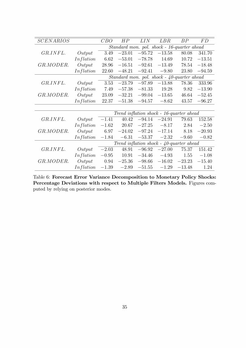
SCENARIOS CBO HP LIN LBR BP FDStandard mon. pol. shock - 16-quarter ahead

GR:INFL: Output 3:49 �23:01 �95:72 �13:58 80:08 341:70Inflation 6:62 �53:01 �78:78 14:69 10:72 �13:51

GR:MODER: Output 28:96 �16:51 �92:61 �13:49 78:54 �18:48Inflation 22:60 �48:21 �92:41 �9:80 23:80 �94:59

Standard mon. pol. shock - 40-quarter aheadGR:INFL: Output 3:53 �23:79 �97:89 �13:88 78:36 333:96

Inflation 7:49 �57:38 �81:33 19:28 9:82 �13:90GR:MODER: Output 23:09 �32:21 �99:04 �13:65 46:64 �52:45

Inflation 22:37 �51:38 �94:57 �8:62 43:57 �96:27

Trend in�ation shock - 16-quarter aheadGR:INFL: Output �1:41 40:42 �94:14 �24:91 79:63 152:58

Inflation �1:62 20:67 �27:25 �8:17 2:84 �2:50GR:MODER: Output 6:97 �24:02 �97:24 �17:14 8:18 �20:93

Inflation �1:84 �6:31 �53:37 �2:32 �9:60 �0:82Trend in�ation shock - 40-quarter ahead

GR:INFL: Output �2:03 48:91 �96:92 �27:00 75:37 151:42Inflation �0:95 10:91 �34:46 �4:93 1:55 �1:08

GR:MODER: Output 0:94 �25:36 �98:66 �16:02 �23:23 �15:40Inflation �1:39 �2:89 �51:55 �1:29 �13:48 1:24

Table 6: Forecast Error Variance Decomposition to Monetary Policy Shocks:Percentage Deviations with respect to Multiple Filters Models. Figures com-puted by relying on posterior modes.

35