Universita degli Studi di Milano

Facolta di Scienze Matematiche, Fisiche e Naturali

Laurea Triennale in Fisica

Static polarizability of clustersof Ionic Liquid

Relatore: Prof. Giovanni Onida

Correlatore: Dott. Nicola Manini

Annalisa Paroni

Matricola n◦ 688825

A.A. 2008/2009

Codice PACS: 36.40.-c

Static polarizability of clusters of

Ionic Liquid

Annalisa Paroni

Dipartimento di Fisica, Universita degli Studi di Milano,

Via Celoria 16, 20133 Milano, Italia

June 04, 2009

Abstract

We evaluate static polarizability of small ionic liquid clusters by means

of molecular dynamics simulations, using the DL POLY package. The po-

larizability is obtained in two ways: by the direct evaluation of the dipole

moment induced as a response to a static electric field and by means of

the fluctuation-dissipation relation applied to a zero-field numerical exper-

iment.

Advisor: Prof. Giovanni Onida

Co-Advisor: Dr. Nicola Manini

3

Contents

1 Introduction 6

1.1 Ionic Liquids . . . . . . . . . . . . . . . . . . . . . . . . . . . . . 6

1.2 The molecule . . . . . . . . . . . . . . . . . . . . . . . . . . . . . 7

1.2.1 The cation . . . . . . . . . . . . . . . . . . . . . . . . . . . 7

1.2.2 The anion . . . . . . . . . . . . . . . . . . . . . . . . . . . 9

2 The model 10

2.1 Statistical Mechanics . . . . . . . . . . . . . . . . . . . . . . . . . 10

2.1.1 Thermal averages and fluctuations . . . . . . . . . . . . . 10

2.1.2 Computational details . . . . . . . . . . . . . . . . . . . . 12

2.2 Units . . . . . . . . . . . . . . . . . . . . . . . . . . . . . . . . . . 12

3 Technical implementation 14

3.1 Classical Molecular Dynamics . . . . . . . . . . . . . . . . . . . . 14

3.2 The force field . . . . . . . . . . . . . . . . . . . . . . . . . . . . . 15

3.3 Time-integration algorithm . . . . . . . . . . . . . . . . . . . . . . 16

3.3.1 The Verlet algorithm . . . . . . . . . . . . . . . . . . . . . 17

3.4 Total energy . . . . . . . . . . . . . . . . . . . . . . . . . . . . . . 17

3.5 Temperature . . . . . . . . . . . . . . . . . . . . . . . . . . . . . . 18

3.6 Thermostat: the Nose-Hoover algorithm . . . . . . . . . . . . . . 18

3.7 The DL POLY package . . . . . . . . . . . . . . . . . . . . . . . . 19

4

4 Results 20

4.1 NVT simulations . . . . . . . . . . . . . . . . . . . . . . . . . . . 20

4.2 The calculation of polarizability . . . . . . . . . . . . . . . . . . . 21

5 Discussion and Conclusion 27

Bibliography 28

5

1 Introduction

1.1 Ionic Liquids

Ionic Liquids (ILs) (Refs. [4, 5, 6, 7, 8, 9] are organic materials which consist

entirely of ions. ILs differ from molten salts mostly in their melting point: ILs

are liquid below 100 ◦C, but some of them are liquid at still lower temperatures,

such as Room Temperature Ionic Liquids (RTILs).

Figure 1: Examples of ionic liquids. The different colors seem due to

impurities. Despite what the vivid colors may let one think, impurity

concentrations are minimal.

ILs, see Fig. 1, have turned out very interesting especially for ”green chemistry”

[15] as alternatives to the traditional organic solvents, because their physical-

chemical properties can be easily changed by varying the structure of the organic

cation and replacing the anion, thus obtaining an extremely large family of ILs.

Moreover, most ionic liquids are biodegradable and not toxic.

Several properties of ILs make them interesting for many applications. The

low melting temperature was, chronologically, the first property that brought

ILs to industrial attention. They have been employed as electrolytes in thermal

batteries [16], with the great advantage of decreasing the otherwise high work-

ing temperature of such devices. Being constituted entirely of ions, ILs have a

much higher ionic concentration than normal electrolytes, thus they are useful in

6

all those devices that exploit electrolytes, i.e. electrochemical super-capacitors

and Gratzel cells or dye-sensitized solar cells (DSSC) [17, 25]. Their extremely

low vapor pressure, due to the strong long-ranged Coulombic interaction, avoids

evaporation at room temperature, optimizing their waste as solvents in chemical

processes. Thanks to the low vapor pressure, also ”non-intrinsically green” ILs

(such as those containing alkaloids as cations or cyanide as anion) are safer for

industrial use, also because they are often non-flammable [10]. Waste of chemical

processes can be further reduced thanks to the fact that ILs are designer solvents,

thus, in principle, one could design an IL solvent to optimize each given reaction.

Furthermore, ILs are regenerable [14]. Thanks to their negligible volatility, non-

flammability, low melting temperature and high thermal stability, ILs seem also

fairly good lubricants, especially in vacuum and in space applications.

1.2 The molecule

The goal of the present work is to evaluate the static polarizability of small clus-

ters of ionic liquid [bmim]+[NTf2]− by means of Molecular Dynamics, probably

smaller than those which could be generated by spray techniques. Polarizability

represents the attitude of a charge distribution of being distorted from its original

shape by an external electric field due to the displacement of ions or dipoles. This

quantity affects many physical and physical-chemical properties. The study of

polarizability is useful to predict the behavior of an ionic liquid when employed

in devices that work in presence of electrical fields.

1.2.1 The cation

The [bmim]+ (1-butyl-3-methylimidazolium [C8H15N2]+) cation, shown in Fig. 2,

is member of the dialkylimidazolium cation family [11, 12, 13]. The substituents

at nitrogen of [bmim]+ are of course methyl and butyl, i.e. alkyl chains composed

of one and four carbon atoms, respectively. The low melting point of ILs con-

taining this cation finds explanation in the delocalization of the positive charge

around the imidazolium ring (Fig. 3) and the asymmetry of the molecular ion.

7

Figure 2: Ball-and-stick model of [bmim]+ anion. Letters on the balls

indicate the chemical symbols of atoms.

Figure 3: Ball-and-stick model of the imidazolium ring.

8

1.2.2 The anion

The [NTf2]− (bistriflimide [(CF3SO2)2N]−) anion, displayed in Fig. 4, is widely

used in the lab, since it is less toxic and more stable than more ”traditional” ions.

Figure 4: Ball-and-stick model of [NTf2]− anion. Letters on the balls

indicate the chemical symbols of atoms.

Specifically, [bmim]+[NTf2]− is considered one of the archetype systems by the

ILs scientific community and it is being studied by P. Milani’s experimental group

at University of Milan [2], in collaboration with QUILL (Queen’s University Ionic

Liquids Laboratories) at the Queen’s University of Belfast [3].

9

2 The model

2.1 Statistical Mechanics

The object of this work is the static polarizability of IL clusters, which is a

thermodynamical observable to treat with statistical mechanics. We start to set

up briefly the notation for our calculations. We will describe specifically the

fluctuation-dissipation theorem [23] in the form we used to predict the linear re-

sponse of a system from its reversible fluctuations in thermal equilibrium. The

Fluctuation dissipation theorem is very useful to predict the non-equilibrium be-

havior of a system from its reversible fluctuations in thermal equilibrium. This

extremely general theorem makes use of the assumption that a system in its

thermodynamic equilibrium, when submitted to perturbations weak enough that

rates of relaxation remain unchanged, produces a response analogous to a spon-

taneous fluctuation. Actually, this theorem quantifies the relation between the

fluctuations in a system at thermal equilibrium and the response of the system

to applied perturbations.

2.1.1 Thermal averages and fluctuations

Consider Boltzmann statistic, where we use the trace notation to represent the

summation over all states of either a classical or a quantum system. In fact we

deal only with classical systems in this work. For classical systems, we have:

Tr X =

∫

X dΓ , (1)

where dΓ represents an infinitesimal volume in phase space.

With a system described by a probability distribution f(q, p) in phase space,

the average value of an arbitrary function A of the system state is given by

〈A〉 = Tr {A(q, p) f(q, p)} , (2)

where angular brackets denote the averaging over the ensemble. The probability

distribution is given by the equilibrium Boltzmann distribution

f(q, p) =exp (−βH(q, p))

Tr(exp (−βH(q, p))), (3)

10

so that the ensemble average equals

〈A〉 = Tr {A(q, p) f(q, p)} =Tr{

Ae−βH}

Tr e−βH, (4)

where β = 1

kBT, kB is the Boltzmann constant, and T is the absolute temperature

in Kelvin.

When an external electric field E is applied to a polarizable system, it couples

to the instantaneous electric dipole d with energy

U = −d · E0 (5)

This situation causes the system to distort and develop a finite average electronic

dipole as a reaction to this external perturbation. According to Eq. (2), when

equilibrium is reached, the thermodynamic average electric dipole is given by

〈d〉 =Tr(exp(−β(H0 − d · E))d)

Tr(exp(−β(H0 − d · E))). (6)

In the weak-field linear-response region, the polarizability represents capability of

the system to react to the external field application, generating an electric dipole:

〈d〉 = αE , (7)

which in components is:

〈di〉 =∑

j

αij Ej . (8)

In other terms, the polarizability estimates the variation of the dipole thermody-

namical average per unit applied electric field. In formula:

α =∂〈d〉

∂E

∣

∣

∣

E=0

(9)

Computing the derivative, we apply the fluctuation dissipation theorem and we

obtain:

α =Tr( ∂

∂Eexp(−β(H0 − d ·E)) ⊗ d)(Tr(exp(−β(H0 − d · E))))

(Tr(exp(−β(H0 − d · E))))2

−Tr(exp(−β(H0 − d ·E))d) ⊗ Tr( ∂

∂Eexp(−β(H0 − d · E))

(Tr(exp(−β(H0 − d · E))))2

∣

∣

∣

∣

∣

E=0

= βTr(exp(−βH0)d⊗ d)

Tr(exp(−βH0))

− β

(

Tr(exp(−βH0)d)

Tr(exp(−βH0))⊗

Tr(exp(−βH0)d)

Tr(exp(−βH0))

)

(10)

11

or, more synthetically, in terms of the definition of thermodynamical average:

α = β〈d⊗ d〉 − β〈d〉 ⊗ 〈d〉 . (11)

In components this means:

αij =1

kBT(〈didj〉 − 〈di〉〈dj〉) . (12)

This relation provides an explicit connection between the linear-response polar-

izability α and the thermal fluctuations of the dipole d.

2.1.2 Computational details

Our molecular-dynamics simulations provide us a sampling of the positions of all

atoms at subsequent times. Each atom carries a known time-independent point

charge. To compute the electric dipole from the molecular-dynamics trajectory

we use the definition of the total dipole

d =∑

i

qi(ri −R) (13)

where d is the electric dipole, qi the charge of the i-th atom, ri its position and

R is an arbitrary reference coordinate. Since in our specific situation there is

no net charge (the neutral droplets are made of the same number of cations as

of anions),∑

i qi = 0, then the electric dipole moment does not depend on the

arbitrary choice of R. Accordingly we take R = 0. To calculate the averages of

Eq.(2) we replace the summation over all phase space weighted by the Boltzman

distribution by a time integration. For example the average dipole moment is

evaluated as

〈d〉 ≃1

Nt

tmax∑

t=tmin

d(t) . (14)

in terms of the Nt recorded time frames. Similar expressions are used to evaluate

the correlation functions of Eq.(12).

2.2 Units

The definition, Eq.(7), of polarizability indicates its units. Since (Eq.(5))

[d · E] = [Energy] (15)

12

by eliminating E in favor of α (Eq. (7)), we get:

[α] =[d]2

[Energy]=

[Charge]2[Length]2

[Energy](16)

Accordingly, in the SI system of units, α is measured in C2m2

J, or equivalently

Cm2

V.

The electric dipole, as computed from the simulation data, is expressed in

terms of elementary charge units qe = 1.602 · 10−19 C times A= 10−10 m. To

convert the electric dipole into Cm we must therefore multiply by 1.602 · 1029

and express energies (for example the kBT energy in Eq.(12)) in J units. In the

literature it is customary to express polarizabilities divided by the electromagnetic

constant ε0, which is measured in C2

Jm, so that α

ε0

is a volume, which can be

measured, e.g., in m3, or in A3.

13

3 Technical implementation

The present section provides a brief description of the tools we used to work our

goal out, such as the elements of classical MD and the DL POLY package [18]

that we use.

3.1 Classical Molecular Dynamics

Classical Molecular Dynamics (MD) [1, 19, 20] is a computer simulation technique

where the time evolution of a set of interacting atoms is followed by integrating

their equations of motion, specifically Newton’s law:

Fi = miai (17)

for each atom i of a system constituted by N atoms. This means that MD is a

deterministic technique, so that, starting from an initial set of given positions and

velocities, the subsequent time evolution is in principle completely determined.

Actually, the finiteness of the integration time-step and arithmetic rounding errors

cause the computed trajectory to eventually deviate from the true one.

Due to the ergodic principle molecular dynamics is a statistical method: it is

a way to obtain a set of configurations distributed according to some statistical

distribution function or statistical ensemble. An example is the microcanonical

ensemble, corresponding to a probability density in phase space where the total

energy E is maintained constant:

δ(H(Γ) − E) , (18)

where H(Γ) is the Hamiltonian and Γ represents the set of positions and momenta.

δ is the Dirac function, selecting only those states which have a specific energy

E. The integration of Newton’s law (17) is compatible with the microcanonical

ensemble.

Another example is the canonical ensemble, where temperature T is main-

tained constant and the probability density is the Boltzmann function

exp

(

−H(Γ)

kBT

)

. (19)

According to Eq.(2), physical quantities are represented by averages over con-

figurations distributed according to a given statistical ensemble. A trajectory

14

obtained with MD provides such a set of configurations. Therefore the measure-

ment of a physical quantity by simulation is simply obtained as the arithmetic

average of the various instantaneous values assumed by that quantity during the

MD run.

Statistical physics is the link between the microscopic dynamics and thermo-

dynamics. In the limit of very long simulation times, one could expect the phase

space to be significantly sampled and, in that limit, this averaging process would

yield the exact thermodynamic properties, allowing to evaluate, say, the phase

diagram of a specific material.

Beside this ”traditional” use, MD is also used for other purposes, such as

studies of non-equilibrium processes and as an efficient tool for optimization of

structures overcoming local energy minima (simulated annealing).

3.2 The force field

Using the correct model for the physical system is of fundamental importance to

run a meaningful simulation. For a molecular dynamics simulation this amounts

to choosing the potential: a function V (r1, . . . , rN) of the positions of the nuclei,

representing the potential energy of the system when the atoms are arranged

in that specific configuration. This function is translationally and rotationally

invariant. It is a function of the relative positions of the atoms with respect to

each other, rather than from the absolute positions.

Forces are then derived as the gradients of the potential with respect to atomic

displacements:

Fi = −∇riV (r1, . . . , rN) . (20)

This form implies the presence of a conservation law for the total energy E =

K + V , where K is the instantaneous kinetic energy.

The simplest choice for V is to write it as a sum of pairwise interactions:

V (r1, . . . , rN) =∑

i

∑

j>i

φ(|ri − rj|) . (21)

The clause j > i in the second summation has the purpose of considering each

atom pair only once.

15

The force field used in the present work however is much more complicated

than this. In addition to pairwise interactions of the type (21) (which also include

Coulomb interactions between atomic charges), it also contains terms which de-

pend on the angles and dihedral angles, as needed to keep the flexible shapes of

the molecular ions. The details of the AMBER-type force field are given in Refs.

[22, 24].

3.3 Time-integration algorithm

The engine of a MD program is its integration algorithm, required to integrate

the equation of motion of the interacting particles and follow their trajectory.

Time integration algorithms are based on finite difference methods, where time is

discretized on a finite grid, the time step ∆t being the distance between consec-

utive points on the grid. Knowing the positions and possibly some of their time

derivatives at time t, the integration scheme gives the same quantities at a later

time t + ∆t. By iterating the procedure, the time evolution of the system can be

followed for long times.

Of course, these schemes are approximate and there are errors associated with

them, which in principle can be reduced by decreasing ∆t.

The general backbone of a MD simulation can be represented in the following

step procedure:

1. start with an initial atomic configuration and initial velocities;

2. compute the interatomic forces for the current configuration;

3. update the atomic positions and velocities according to the integration al-

gorithm;

4. iterate step 2 and step 3 Nstep times, until Nstep ·∆t equals the desired total

integration time.

One of the most popular integration methods for MD calculations is the Verlet

algorithm, presented briefly below.

16

3.3.1 The Verlet algorithm

The basic idea of this algorithm is to write two third-order Taylor expansions for

the positions r(t), one forward and one backward in time. Calling v the velocities,

a the accelerations and b the third order derivatives of r with respect to t:

r(t + ∆t) = r(t) + v(t)∆t +1

2a(t)∆t2 +

1

6b(t)∆t3 + O(∆t4) (22)

r(t − ∆t) = r(t) − v(t)∆t +1

2a(t)∆t2 −

1

6b(t)∆t3 + O(∆t4) (23)

Adding the two expressions gives

r(t + ∆t) = 2r(t) − r(t − ∆t) + a(t)∆t2 + O(∆t4) . (24)

This is the basic form of the Verlet algorithm [1, 21].

Since the equations to be integrated are Newton’s equations, a(t) is simply the

force divided by the mass and the force is in turn a function of the position r(t),

Eq.(20)

a(t) = −∇V (r(t))

m. (25)

It is easily to see that the algorithm, when evolving the system by ∆t, is quite

accurate, its error being of order ∆t4.

This algorithm is at the same time simple to implement, reliable and stable,

which explains its large popularity among MD simulators. A problem with this

version of the Verlet algorithm is that velocities are not directly generated.

To overcome this difficulty, some variants of the Verlet algorithm have been

developed. They give rise to exactly the same trajectory and differ in what

variables are stored in memory and at what times. The leap-frog algorithm is

a better implementation of the Verlet algorithm and the velocity Verlet scheme

is an even better one still, where positions, velocities and accelerations at time

t + ∆t are obtained from the same quantities at time t.

3.4 Total energy

The total energy E = K + V is a conserved quantity in newtonian dynamics. It

can be computed at each time-step in order to check its actual conservation with

time. In practice small fluctuations in the total energy often occur due to errors

17

in time integration. They can be reduced by lowering the time-step, if considered

excessive.

Slow drifts of the total energy are also sometimes observed in long runs. Again,

the cause could be an excessive time-step. Drifts are more disturbing than fluctu-

ations because the thermodynamic state of the system is changing together with

the energy, therefore time averaging over the run do not refer to a single state.

Drifts over long runs could be prevented by breaking the long run into smaller

runs and restoring the energy to the nominal value between one piece and the

next. A common mechanism to adjust the energy is to modify the kinetic energy

via rescaling of velocities.

3.5 Temperature

The temperature T is directly related to the kinetic energy by the equipartition

formula, which assigns an average kinetic energy 1

2kBT per degree of freedom:

K =3

2NkBT . (26)

An estimate of the temperature is obtained directly from the average kinetic

energy

K(t) =1

2

∑

i

mi|vi(t)|2 . (27)

For practical purposes, it is also common to define an ”instantaneous tempera-

ture” T kin(t), proportional to the instantaneous kinetic energy K(t).

3.6 Thermostat: the Nose-Hoover algorithm

When running a MD simulation in the canonical (NVT) ensemble, the system

must be coupled with a heat bath to ensure that the average temperature is

maintained close to the requested temperature T . In such a situation, some

modifications to the equations of motion are required.

In this work we use the Nose-Hoover algorithm, which generates smooth, de-

terministic and time-reversible trajectories in the canonical ensemble. Newton’s

equations of motion are modified as follows:

dr(t)

dt= v(t)

dv(t)

dt=

f(t)

m− χ(t)v(t) (28)

18

where χ is called friction coefficient and is controlled by the first order differential

equationdχ(t)

dt=

fkB

Q(T kin(t) − T ) (29)

where Q = fkBTτ 2T is the effective ”mass”, τT is a specific time constant, f is

the number of freedom degrees, T kin(t) is the instantaneous temperature of the

system represented by the kinetic temperature function obtained by Eq. (26)

and (27). This dynamics involves a conseved quantity derived from the extended

Hamiltonian of the system, which, to within a constant, equals the Helmholtz

free energy:

HNV T (t) = U + K +1

2Qχ(t)2 +

Q

τ 2T

∫ t

0

χ(s)ds . (30)

3.7 The DL POLY package

Our simulations are carried out using DL POLY [18], which is a parallel simula-

tion tool developed by W. Smith and T. R. Forester at Daresbury Laboratory.

DL POLY is a package of subroutines, programs and data files designed to

perform MD simulations of macromolecules, polymers, ionic systems and other

molecular and atomic systems on a distributed memory architecture of parallel

computers. The DL POLY force-field includes all common forms of non-bonded

atom-atom, Coulombic, valence angle, dihedral angle, inversion, Tersoff and met-

als potentials. In addition to the molecular force-field, also use of an external

force-field is allowed. It is possible to select the ensemble to be used: canonical

(NVT), microcanonical (NVE) and NVP; and it is possible to use thermostats

and barostats. A wide choice of PBCs is available: no PBCs, slab (x, y peri-

odic, z non periodic), cubic PBCs, orthorhombic PBCs, etc. In DL POLY two

versions of the Verlet integration algorithm are implemented: the velocity Ver-

let and the leap-frog. In our simulations we adopt the leap-frog (LF) algorithm

and an integration time-step ∆t = 1 fs: it guarantees a fair conservation of the

constant of motion for the NVT ensemble. Typical values used for the other

parameters required by DL POLY are: rcut = 12 A is the cutoff for short-ranged

forces, rvdwcut = 9 A for van der Waals forces cutoff, τT = 0.2 ps for thermostat

relaxation time, related to its mass Q. We compute the long-range part of the

electrostatic interactions by means of the Ewald-summation method. We set

Ewald sum precision to ε = 10−5, so that Ewald parameters are automatically

optimized.

19

4 Results

We report and analyze the data obtained by means of MD simulations of two

small droplets of the IL [bmim]+[NTf2]−. The droplets considered in this work

have two sizes: a smaller one consists of five anion-cation pairs and a larger one

of ten anion-cation pairs.

Firstly we present the preliminary NVT simulations ran to obtain a reason-

able starting configuration for the droplets. Secondly we describe NVE simula-

tions providing the useful data to compute the static polarizability, and lastly we

present the obtained results for polarizability.

4.1 NVT simulations

First of all, a reasonable starting configuration is needed. Starting from the

configuration of a single anion-cation pair, we translate it five times by 7 A and

run a proper simulation in order to let all the atoms interact and join together

into a single droplet. This is done in the canonical ensemble, within a box of

L = 100 A, at T = 300 K for 10 ps. To thermalise the system, we run a short

simulation (100 ps) at T = 400 K and we obtain a useful final configuration for

the five-pair droplet, confined in the same cubic box of side L = 100 A with

PBCs.

The so obtained droplet has a large angular momentum which may affect the

computation of α, so we run some further short simulations (100 ps) lowering the

temperature at each simulation, one after the other, starting the next simulation

from the final configuration of the previous one. Lowering the temperature below

1 K means freezing the system, which in turn means that the kinetic energy is

negligibly small and the angular momentum is null. From this frozen configura-

tion we bring the system back to 400 K through intermediate NVT steps. While

warming, the droplet again acquires an acceptable angular momentum, so the

final configuration of the warming sequence, after a 100 ps equilibration run at

T = 400 K, is a good starting point for further NVE simulations. The initial

configuration of the five-pair droplet is displayed in Fig. 5.

We then build a starting configuration for the ten-pair droplet by duplicat-

ing the five-pair droplet, translated along the z axis by 18 A. A 100 ps NVT

simulation is then sufficient to obtain a single roughly round droplet. The final

20

Figure 5: Ball-and-stick model of the five-pair droplet initial config-

uration. Dark blue, light blue, dark yellow, light yellow, red and cyan

indicate respectively N, F, S, C, O and H.

configuration of this run is the starting point for a 100 ps simulation in a larger

box and the initial configuration used for the longer NVE simulations. This initial

configuration is displayed in Fig. 6.

Because our droplets are very small, DL POLY does not perform well without

a simulation box, thus we adopt a very large cubic box of 300 × 300 × 300

A3. We ran simulations in a larger box to evaluate the possible effects of the

repeated-cell geometry on the computed polarizability. We expect that, in the

small box, the droplets could appear more polarizable than in the large one,

because interacting induced dipoles could influence the computed polarizability

value. The dipole interaction decreases as 1

r3 , thus a big box should reduce

strongly this effect. Actually, results seem to point out that polarizability is the

same when computed in the smaller box and in the larger one, thus we will present

only the results concerning simulations in the smaller box.

4.2 The calculation of polarizability

To compute the electric dipoles and polarizability we run rather long NVE sim-

ulations, to beat the statistical fluctuations.

21

Figure 6: Ball-and-stick model of the ten-pair droplet initial configu-

ration. Colors codes atoms like in Fig. 5.

A first set of simulations involves no external electric field and uses Eq.(12)

to evaluate the static polarizability. We then re-determine the polarizability by

means of Eq.(7) by running simulations with five different values of an applied

external electric field.

We use the positions and charges of the atomic configurations at snapshots

taken at 1 ps interval (i.e. every 1000 simulation steps) to compute the instan-

taneous dipole moment by means of Eq.(13), and then, by averaging, the mean

dipole and its fluctuation tensor 〈d ⊗ d〉 as in Eq. (12). In the zero-field simu-

lations we expect the average dipole value to be close to zero and this is indeed

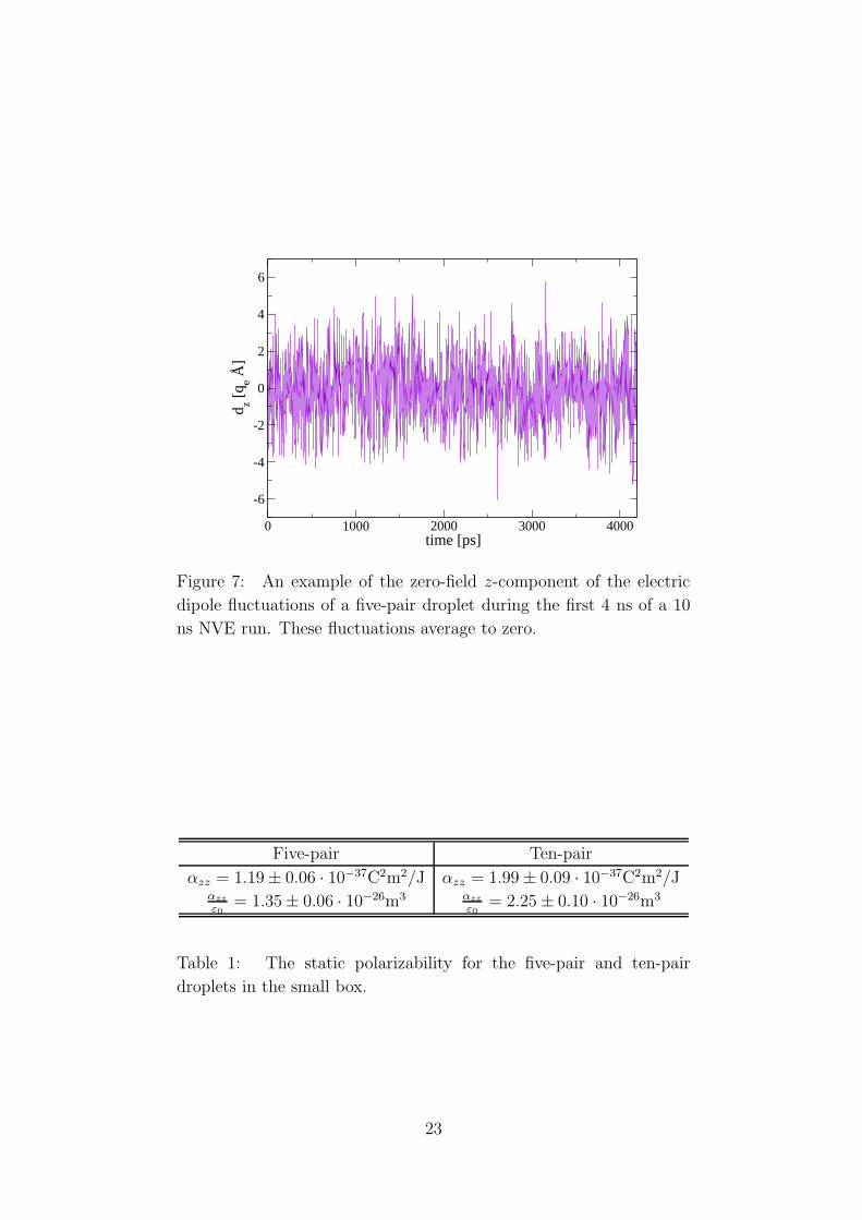
what simulations show. Figure 7 shows the dipole oscillations for the first 4 ns of

the 10 ns run of a five-pair droplet.

Table 1 reports the obtained values of the computed polarizability of the

droplets of two different sizes. Polarizability is given m3, as discussed in Sec.

2.2.

In the second set of simulations we apply an electric field to compute the

polarizability by means of Eq. (7). The z-directed electric field allows us to

evaluate the zz component of the α tensor.

22

0 1000 2000 3000 4000time [ps]

-6

-4

-2

0

2

4

6

d z [qe Å

]

Figure 7: An example of the zero-field z-component of the electric

dipole fluctuations of a five-pair droplet during the first 4 ns of a 10

ns NVE run. These fluctuations average to zero.

Five-pair Ten-pair

αzz = 1.19 ± 0.06 · 10−37C2m2/J αzz = 1.99 ± 0.09 · 10−37C2m2/Jαzz

ε0

= 1.35 ± 0.06 · 10−26m3 αzz

ε0

= 2.25 ± 0.10 · 10−26m3

Table 1: The static polarizability for the five-pair and ten-pair

droplets in the small box.

23

When applying an external electric field, the first ps of the simulation are

employed by the system to react to the new situation, so they must not be

included in averages to avoid systematic errors in the computed polarizability.

Figure 8 displays the transient from a situation of null electric field to a situation

of non-zero applied electric field.

0 50 100 150time [ps]

-2

0

2

4

6

8

10

d z [qe Å

]

Figure 8: The transient after a simulation of no external electric field,

when an external electric field Ez = 5 ·108 V/m is turned on.

In Fig. 9 the dipole z component is shown as a function of the electric field

z component, the lines representing polarizability. As the goal of this work is

to compute polarizability as the linear response to the application of an electric

field, we compute the polarizability by means of a linear fit of our data. The

resulting values for polarizability are collected in Table 2.

Five-pair Ten pair

αzz = 1.28 ± 0.08 · 10−37(C2m2/J) αzz = 2.23 ± 0.09 · 10−37(C2m2/J)αzz

ε0

= 1.45 ± 0.09 · 10−26m3 αzz

ε0

= 2.52 ± 0.10 · 10−26m3

Table 2: Static polarizability for the five-pair and ten-pair droplets in

the small box, computed by means of a linear fit of the average dipole

induced by an electric field of up to 5 ·108 V/m, as shown in Fig. 9.

The values of polarizability are systematically slightly larger when computed in

the presence of applied electric field. Anyway they are compatible within 2σ with

the polarizability computed without electric field. As expected, larger systems

24

0 2×108

4×108

6×108

8×108

1×109

Ez [V/m]

0

1×10-28

2×10-28

<d z>

[Cm

]

10-pair droplet5-pair droplet5-pair droplet fit10-pair droplet fit

Figure 9: The electric dipole component dz as a function of the electric

field component Ez for the five-pair droplet (circles) and the ten-pair

droplet (diamonds). The lines are linear fits (with null intercept) of

the simulation data up to Ez = 5 ·108 V/m.

25

are more polarizable than smaller ones, as they are capable of distorting and

polarizing more. This also could be the reason why for the ten-pair droplet the

linearity of the relation between dipole and field is worse than that regarding the

five-pair droplet. However we find that the polarizability of the ten-pair cluster

is less than twice that of the five-pair cluster.

The 109 V/m external field turns out to be excessive, as the droplets disinte-

grate within few ps after the beginning of the simulations. This is why excluded

those points from the linear fit. Indeed those points deviate considerably from

linearity.

26

5 Discussion and Conclusion

Molecular-dynamics simulations are a valid tool to determine the static polariz-

ability. Dipole fluctuations are indeed useful for the determination of the polariz-

ability via the fluctuation-dissipation theorem, without the need of the application

of an external field. In fact, one could even determine the frequency-dependency

of the polarizability, by Fourier transforming the dipole-dipole time-dependent

correlation functions 〈d(t) ⊗ d(t + τ)〉.

The present calculation grab the bulk of the polarizability, the part due to the

displacement of the charged atoms in the field. The atomic molecular polariz-

ability part is completely omitted in our calculation, but it is expected to be a

fairly small fraction in these IL systems.

The calculations employing an external field need to involve an extremely large

one, a few orders of magnitude larger than could be applied in a lab experiment,

but this is necessary to beat the huge dipole fluctuations in the simulations and

to obtain meaningful average values within reasonable simulation times.

27

References

[1] F. Ercolessi, A molecular dynamics primer, 1997

http://www.fisica.uniud.it/˜ercolessi/md/ .

[2] S. Bovio, A. Podesta, C. Lenardi, and P. Milani, J. Phys. Chem. B 113, 6600

(2009).

[3] P. Ballone, C. Pinilla, J. Kohanoff, and M. G. Del Popolo, J. Phys. Chem. B

111, 4938 (2007).

[4] K. R. Seddon, J. Chem. Tech. Biotechnol. 68, 351 (1999).

[5] J. D. Holbrey and K. R. Seddon, Clean Products and Processes 1, 223 (2007).

[6] K. R. Seddon, Nature Materials 2, 363 (2003).

[7] V. Plechkova and K. R. Seddon, Chem. Soc. Rev. 37, 123 (2008).

[8] R. D. Rogers and K. R. Seddon, Science 302, 792 (2003).

[9] G. Fitzwater, W. Geissler, R. Moulton, N. V. Plechkova, A. Robertson, K. R.

Seddon, J. Swindall, and K. Wan Joo, Ionic Liquids: Sources of Innovation,

Report Q002, January 2005, QUILL, Belfast.

[10] T. Welton, Chem. Rev. 99, 2071 (1999).

[11] J. S. Wilkes, J. A. Levisky, R. A. Wilson, and C. L. Hussey,, Inorg. Chem.

21, 1263 (1982).

[12] J. R. Sanders, E. H. Ward, and C. L. Hussey J. Electrochem. Soc. 133, 325

(1986).

[13] C. L. Hussey, Pure Appl. Chem. 60, 1763 (1988).

[14] BASIL–The first commercial process using ionic liquids,

http://www.corporate.basf.com/en/innovationen/preis/2004/basil.htm.

[15] P. Anastas and J. Warner, Twelve Principles of Green

Chemistry, United States Environmental Protection Agency.

http://epa.gov/greenchemistry/pubs/principles.html.

[16] J. S. Wilkes, Green Chemistry 4, 73 (2002).

[17] M. Gratzel, J. Photochem. Photobiol. C 4, 145 (2003).

28

[18] W. Smith, T. R. Forester, and I. T. Torodov, The DL POLY 2 User Manual,

Version 2.19, Daresbury, Warrington, UK, 2008.

[19] M. P. Allen and D. J. Tildesley, Computer Simulation of Liquids Clarendon

Press, Oxford, 1987.

[20] D. Frenkel and B. Smit, Understanding molecular simulation: from algo-

rithms to applications (Academic San Diego, 1996).

[21] L. Verlet, Phys. Rev. 159, 98 (1967).

[22] S. J. Weiner, P. A. Kollman, D. T. Nguyen and D. A. Case J. Comp. Chem.

7, 230 (1986).

[23] K. Huang, Statistical Mechanics, (Wiley, Boston 1987).

[24] M. Cesaratto, Molecular-Dynamics Simulations of Adsorbed Ionic-Liquid

Films. Diploma thesis. Universita degli Studi di Milano, 2008.

[25] F. Borghi, Dye-sensitized solar cells come percorso didattico e strumento

di divulgazione scientifica, Diploma thesis (Universita degli Studi di Milano,

2009).

29