UNIVERSITA DEGLI STUDI DI PADOVA

Dipartimento di Fisica e Astronomia “Galileo Galilei”

Corso di Laurea Triennale in Fisica

Tesi di Laurea

Exploring the Pulse Shape Discrimination capabilities of

the ∆E silicon detectors of the EUCLIDES array

Relatore Laureando

Dr. Alain Goasduff Giovanni Sighinolfi

Correlatori

Dr. Marco Siciliano

Dr. Daniele Mengoni

Anno Accademico 2017/2018

Contents

1 Introduction 2

2 Performances of the CAEN V1730B 42.1 Constant Fraction Discriminator . . . . . . . . . . . . . . . . . . . . . . . . . 52.2 DT5720 analysis . . . . . . . . . . . . . . . . . . . . . . . . . . . . . . . . . . 52.3 V1730B analysis . . . . . . . . . . . . . . . . . . . . . . . . . . . . . . . . . . 6

3 Experimental setup 7

4 Data analysis 84.1 Energy . . . . . . . . . . . . . . . . . . . . . . . . . . . . . . . . . . . . . . . . 84.2 Timing performances . . . . . . . . . . . . . . . . . . . . . . . . . . . . . . . . 13

4.2.1 CFD difference between E and ∆E channels . . . . . . . . . . . . . . . 134.2.2 CFD difference between NeutronWall and ∆E waveforms . . . . . . . 18

4.3 Induced signals and coincidences . . . . . . . . . . . . . . . . . . . . . . . . . 21

5 Comparisons with the simulations 235.1 Calibration check . . . . . . . . . . . . . . . . . . . . . . . . . . . . . . . . . . 235.2 Time of Flight . . . . . . . . . . . . . . . . . . . . . . . . . . . . . . . . . . . 24

6 Conclusions 27

7 References 28

8 LNL Annual Report 29

1

2

1 Introduction

The GALILEO project at Laboratori Nazionali di Legnaro (LNL) aims to explore the nuclearstructure at extreme conditions, such as exotic excited states produced at very low crosssection. The final configuration of the GALILEO array is a 4π high-efficiency ball, madeup of germanium detectors. In its current implementation, only the backward hemisphereand a 90o ring are used, as shown in Fig. 1(a). In order to improve its selectivity, differentancillary devices, which can help to select processes with much higher resolution than simpleγ-detection, are coupled to it: Neutron Wall (which will also be mentioned in this work),NEDA (NEutron Detector Array) and EUCLIDES are some examples. The EUCLIDESarray, pictured in Fig. 1(b), is a silicon ball, with a diameter close to 13 cm, which constitutesa light charged-particles detector. The complete array is made of 55 ∆E-E pentagonal andhexagonal telescopes, which provide a solid angle coverage close to 4π. The silicon thicknessis ∼130 µm and ∼1000 µm for ∆E and E layers respectively and the surface of each telescopeis ∼10 cm2.

Because of the kinematic enlargement of the solid angle in the center of mass frame ofreference for a typical fusion-evaporation reaction (v/c≈5%), the most forward positionedtelescopes have to deal with higher counting rates with respect to the others; thus, 5 of themare segmented in 4 equal parts, with individual electronic processing circuits, to reduce theprobability of pile-up and increase the counting rate capabilities.

The first advantage of the coupling of GALILEO and EUCLIDES array is that, since ina fusion-evaporation process various species are produced in different evaporation channels,simultaneous detection of evapored light particles (such as protons, deuterons, α, etc.) andemitted γ rays can lead to the maximum selectivity. Another considerable benefit is to havethe possibility to reconstruct event-by-event the trajectory of the recoiling nuclei, in order toreduce the Doppler broadening of peaks in the recorded γ-ray spectra.

(a) (b) (c)

Figure 1: The current configuration of the GALILEO array (a), the light charged particles detectorEUCLIDES (b) and the CAEN V1730B 500MS/s digitizer (c)

EUCLIDES has already been used successfully in the past years at LNL in differentGALILEO experiments and it will certainly be an important tool for the forthcoming onesusing radioactive ions beams delivered in the near future by the SPES facility.

In December 2017, 3 E-∆E segments of one forward segmented telescope were connectedto a CAEN V1730B (Fig. 1(c)), which is a 1-unit wide VME module housing 16 channels

3

14-bit 500 MS/s Flash ADC Waveform Digitizer, therefore it is able to take a sample every2 ns, for 16 different channels, at the same time. The configuration of the digitizer in termsof trigger channels, trigger levels, polarity of the input channels etc. are set using a text fileread by the CAEN software WaveDump. The traces from each active channels are dumpedin separated binary files as soon as one of the active channel is triggering.

The aim of the implementation of the new digitizer in the read-out chain of EUCLIDESis to have the possibility to distinguish between α particles and protons stopping in the ∆Elayer. Depending on the kinematics of the reaction and the thickness of the absorber layers,used to prevent the elastic scattering of the beam from reaching the detectors, those eventsstopping in the ∆E can represent more than 50% of the detected particles, thus it would bean important step forward to have the possibility to recover such events. In order to reachthe maximum particle detection efficiency and selectivity in the light charged particle-γ-raysin fusion-evaporation reaction, new methods of particles discrimination for the EUCLIDESarray have been investigated.

The purpose of this work is, therefore, the pulse shape analysis of the waveforms obtainedfrom the 3 telescopes connected to the digitizer. After a preliminar study of the performancesof the CAEN V1730B module, the response of the described setup to an in-beam experimentwill be explored. This will include a detailed study of all the main information obtainablefrom the analysis of the resulting traces, in particular the energy and the timing, which arethe basic elements to attain an identification of the particles stopped in the ∆E layer of thetelescope.

4

2 Performances of the CAEN V1730B

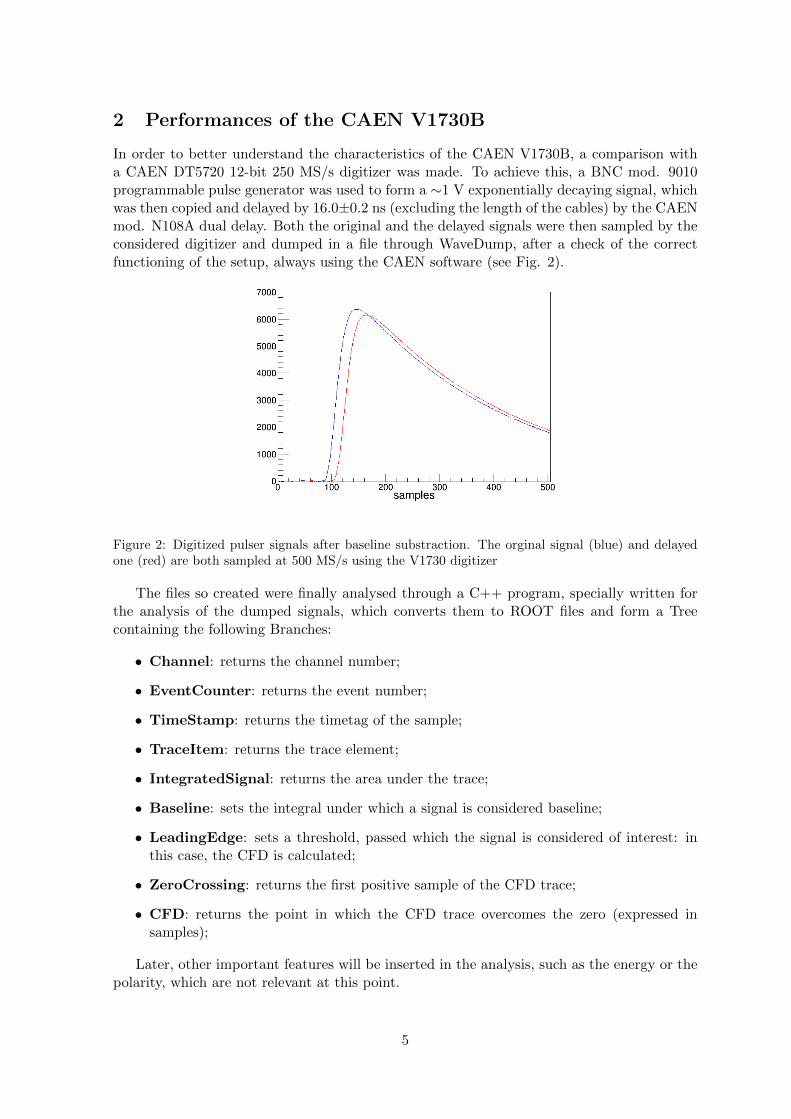
In order to better understand the characteristics of the CAEN V1730B, a comparison witha CAEN DT5720 12-bit 250 MS/s digitizer was made. To achieve this, a BNC mod. 9010programmable pulse generator was used to form a ∼1 V exponentially decaying signal, whichwas then copied and delayed by 16.0±0.2 ns (excluding the length of the cables) by the CAENmod. N108A dual delay. Both the original and the delayed signals were then sampled by theconsidered digitizer and dumped in a file through WaveDump, after a check of the correctfunctioning of the setup, always using the CAEN software (see Fig. 2).

Figure 2: Digitized pulser signals after baseline substraction. The orginal signal (blue) and delayedone (red) are both sampled at 500 MS/s using the V1730 digitizer

The files so created were finally analysed through a C++ program, specially written forthe analysis of the dumped signals, which converts them to ROOT files and form a Treecontaining the following Branches:

• Channel: returns the channel number;

• EventCounter: returns the event number;

• TimeStamp: returns the timetag of the sample;

• TraceItem: returns the trace element;

• IntegratedSignal: returns the area under the trace;

• Baseline: sets the integral under which a signal is considered baseline;

• LeadingEdge: sets a threshold, passed which the signal is considered of interest: inthis case, the CFD is calculated;

• ZeroCrossing: returns the first positive sample of the CFD trace;

• CFD: returns the point in which the CFD trace overcomes the zero (expressed insamples);

Later, other important features will be inserted in the analysis, such as the energy or thepolarity, which are not relevant at this point.

5

2.1 Constant Fraction Discriminator

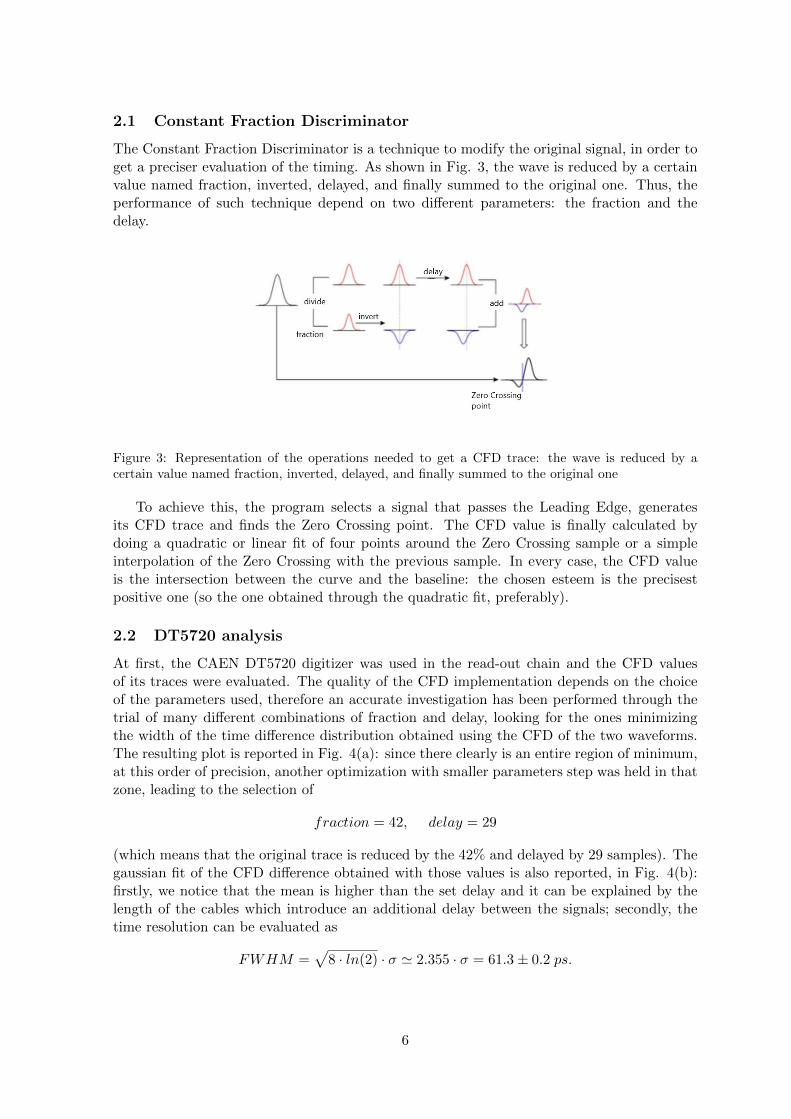
The Constant Fraction Discriminator is a technique to modify the original signal, in order toget a preciser evaluation of the timing. As shown in Fig. 3, the wave is reduced by a certainvalue named fraction, inverted, delayed, and finally summed to the original one. Thus, theperformance of such technique depend on two different parameters: the fraction and thedelay.

Figure 3: Representation of the operations needed to get a CFD trace: the wave is reduced by acertain value named fraction, inverted, delayed, and finally summed to the original one

To achieve this, the program selects a signal that passes the Leading Edge, generatesits CFD trace and finds the Zero Crossing point. The CFD value is finally calculated bydoing a quadratic or linear fit of four points around the Zero Crossing sample or a simpleinterpolation of the Zero Crossing with the previous sample. In every case, the CFD valueis the intersection between the curve and the baseline: the chosen esteem is the precisestpositive one (so the one obtained through the quadratic fit, preferably).

2.2 DT5720 analysis

At first, the CAEN DT5720 digitizer was used in the read-out chain and the CFD valuesof its traces were evaluated. The quality of the CFD implementation depends on the choiceof the parameters used, therefore an accurate investigation has been performed through thetrial of many different combinations of fraction and delay, looking for the ones minimizingthe width of the time difference distribution obtained using the CFD of the two waveforms.The resulting plot is reported in Fig. 4(a): since there clearly is an entire region of minimum,at this order of precision, another optimization with smaller parameters step was held in thatzone, leading to the selection of

fraction = 42, delay = 29

(which means that the original trace is reduced by the 42% and delayed by 29 samples). Thegaussian fit of the CFD difference obtained with those values is also reported, in Fig. 4(b):firstly, we notice that the mean is higher than the set delay and it can be explained by thelength of the cables which introduce an additional delay between the signals; secondly, thetime resolution can be evaluated as

FWHM =√

8 · ln(2) · σ ' 2.355 · σ = 61.3± 0.2 ps.

6

(a) Plot of the values of σ of the gaussian fitof the CFD difference for given fraction (mea-sured in percentage of the original wave) anddelay (in samples)

(b) Gaussian fit of the CFD difference betweentwo equal signals, delayed by 16 ns and sampledby the 250 MS/s digitizer

Figure 4: Search for the optimal CFD parameters and the related gaussian fit, using the CAENDT5720 module

2.3 V1730B analysis

Since the CAEN V1730B is a 500MS/s digitizer, while the DT5720 is a 250 MS/s, it wasassumed, without doing the same test utilized for the construction of Fig. 4(a), that a goodset of CFD parameters, would have been

fraction = 42, delay = 58.

The result of the analysis carried out through this device is shown in Fig. 5. The mean, inthis case, is even higher than the previous one (Fig. 4(b)), because it was necessary to adda ∼1 ns cable in the read-out chain, but the time resolution is more precise, also consideringthat a detailed optimization of the parameters was not achieved (this is justified by the factthat new values needed to be found anyway when elaborating the traces of real particles), infact:

FWHM = 50.3± 0.2 ps

which corresponds to the 82% of the previous outcome.

Figure 5: Gaussian fit of the CFD difference between two equal signals, delayed by 16 ns and sampledby the CAEN V1730B 500 MS/s digitizer

7

3 Experimental setup

In December 2017, an experiment was held at LNL, in which a 250 MeV 64Zn stable beamwas impinging on a ∼0.62 µm 3He target, implanted in a W layer deposited on a thick Aubacking. This target, produced with an innovative procedure, contains a density of ∼0.3·1018

atoms/cm2 of 3He. Traces of 16O have been inferred during the online analysis from the γ-raysspectra. For the simulations of the experiment, presented in section 5.2, this contaminationof the target will be taken into account, and both the processes will be investigated.

During the experiment, the EUCLIDES array was installed in the GALILEO reactionchamber and the CAEN V1730B was used for the readout 3 segments of one of the mostforward telescopes. The even channels 2, 8 and 12 were used for ∆E, while the following oddones (so 3,9 and 13) were connected to the respective E layers. Channel 6 was connected tothe OR signal of the Neutron Wall array. In order to limit the dead time that would comewhen triggering on Neutron Wall array (400 kHz in the present condition), this channel waschosen to be used as a slave of the telescope, i.e. the Neutron Wall channel was recordedonly when it was in coincidence within a 2 µs window with a signal recorded from EUCLIDES.

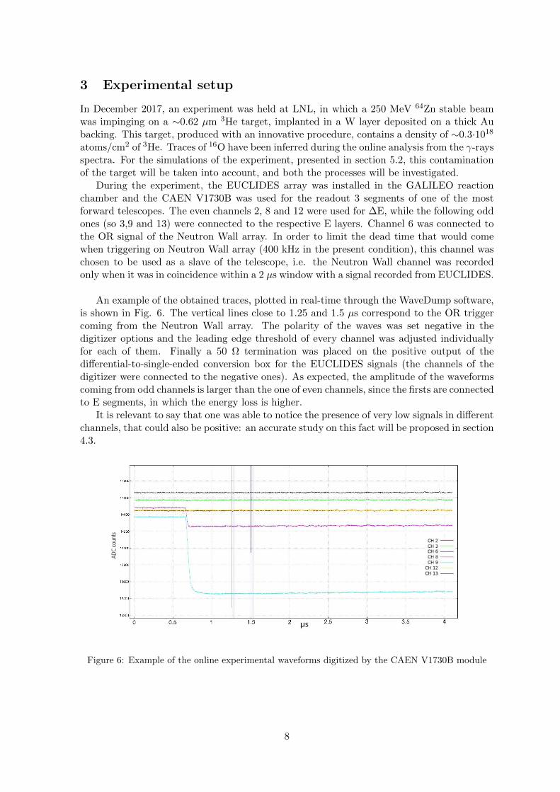
An example of the obtained traces, plotted in real-time through the WaveDump software,is shown in Fig. 6. The vertical lines close to 1.25 and 1.5 µs correspond to the OR triggercoming from the Neutron Wall array. The polarity of the waves was set negative in thedigitizer options and the leading edge threshold of every channel was adjusted individuallyfor each of them. Finally a 50 Ω termination was placed on the positive output of thedifferential-to-single-ended conversion box for the EUCLIDES signals (the channels of thedigitizer were connected to the negative ones). As expected, the amplitude of the waveformscoming from odd channels is larger than the one of even channels, since the firsts are connectedto E segments, in which the energy loss is higher.

It is relevant to say that one was able to notice the presence of very low signals in differentchannels, that could also be positive: an accurate study on this fact will be proposed in section4.3.

Figure 6: Example of the online experimental waveforms digitized by the CAEN V1730B module

8

4 Data analysis

To analyse the waveforms of the in-beam data, additional Branches were added to the Treedescribed in section 2:

• Polarity: returns the polarity of the trace;

• TrapeItem: returns the trapezoidal filter element;

• Energy: returns the energy related to the trace (in arbitrary units), evaluated basingon the trapezoidal filter;

Note also that the program used for the analysis inverts all the negative signals, in orderto simplify the process of evaluation of the CFD and the trapezoidal filter.

A program was also written to merge all the ROOT files containing the information of thedifferent channels into a single one. Doing this, it was finally possible to make comparisonsand operations between, for example, a ∆E channel and the related E one.

4.1 Energy

The trapezoidal filter represents a technique for the synthesis of optimal pulse shapes for highresolution spectroscopy. It was implemented following the equations established by Jordanovet al. in [5] on all the traces overcoming a software threshold. This second threshold has beenset to reduce the processing time, because the CAEN V1730B digitizes all the active channelsand dumps them to disk as soon as one of them is overcoming the hardware trigger threshold.As described in Fig. 7, the parameters of interest for the constitution of the trapezoidal filterare:

• k: sets the length of the rise time of the trapezoid;

• l: represents the sum of the rise time and the flat top length, m, which should be longenough to ensure the possibility to calculate a reasonable value of the energy: in allthe considered cases, this is widely guaranteed, since the program evaluates the energyas the simple mean of 20 samples around the maximum point of the flat top and thenumber of samples taken by the 500MS/s digitizer ensure that this condition is alwayssatisfied;

• k’: sets a delay in the rise time of the trapezoid.

The choice of the best parameters has been achieved through the trial of different combi-nations of them, concluded with the following values:

k = 285 samples, l = 500 samples, k′ = 5 samples.

With these parameters, the trapezoidal filter has the right shape, for channel 13 in par-ticular (see Fig. 8(b)). In general, a worsening of the flat top of the trapezoids is observablewith the decreasing of the amplitude of the waveforms, since the traces become noisier. Con-sequently, the shapes formed for ∆E channels, in most cases, look fragmented on the flat top(see Fig. 8(d)), because they tipically record lower amplitude traces with respect to the Eones, since the energy lost by particles crossing them is also lower. This could be an issue,but, since the oscillation of the flat top was observed to be in the order of 1 unit in the ar-bitrary scale, we assumed that the energy extracted from the trapezoidal filter is acceptable.Other parameters were tried separately for the different channels, but with none of them a

9

Figure 7: Example of trapezoidal filter of an experimental waveform, showing the filter parameters k(rise time), m (flat top) and l (sum of the two)

consistent improvement was observed. For channels 2 and 3, parameters resulting in welldefined trapezoidal shapes were not actually found (see Fig. 8(f)). Also their waveformspresent unforeseen behaviors, especially at low energies, as shown in Fig. 8(e), for examplefor channel 2. Basing on that, we can likely affirm that there was an issue in the electronicprocessing circuit of those channels.

Considering the full statistic, it was possible to form very precise E-∆E matrices for boththe channels pairs 9-8 and 13-12, visible in Fig. 9. The one of channels 3-2 is also reported:for these channels, complete structures are not formed, presenting very little statistic at lowenergy.

In these plots, one can clearly distinguish protons, deuterons, 3He and α particles and seethe punch-through of p, d and α. Also the traces of t, 2p (or its pile-up) and the coincidenceof α particles and protons are slightly visible for channels 9-8 in particular, but they can notbe used for further studies, with this level of statistic. Notice that the number of events of3He considerably increases at high energy: the cause of this is the elastic scattering betweenthe beam and the target, as it will be demonstrated in section 5.1. Since it does not provideenough energy to cause the punch-through of the isotope, the event is not observable in thematrices.

The matrices in Fig. 9 allowed to calibrate the channels, even if for channel 3 only twopoints could be used, since the punch-through of α was not observed. The theoretical values,to compare with the ones obtainable studying the matrices, were evaluated through thePhysical Calulator of LISE++, looking for the maximum energy that the identified particlescan have to be stopped by a 130 µm Si layer (∆E) or a sequence of a 130 µm and a 1000 µmSi layers (∆E+E), in this case selecting only the energy lost in the second one. The first onecorresponds to the value of the intersection between the y axis (i.e. E=0) and the extensiontowards it of the trace of the energy loss , while the second one corresponds to the projectionon x axis of the punch-through point.

The values used for the calibration and the obtained correspondence channel-energy aresummed up in table 1. Note that:

• the errors on the theoretically calculated values are esteemed as half of the precision

10

used for their evaluation;

• the errors on the ∆E values are set as the projection on the y axis of the width of theenergy loss structures;

• the errors on the E values are evaluated as the region in which one could likely position

(a) Trace from channel 13 (E) (b) Top of the trapezoidal filter of the tracereported in Fig. 8(a)

(c) Trace from channel 12 (∆E) (d) Top of the trapezoidal filter of the tracereported in Fig. 8(c)

(e) Trace from channel 2 (∆E) (f) Top of the trapezoidal filter of the tracereported in Fig. 8(e)

Figure 8: Example of E and ∆E waveforms and flat top of their respective trapezoidal filters

11

(a) E-∆E matrix for channels 3-2

(b) E-∆E matrix for channels 9-8

(c) E-∆E matrix for channels 13-12

Figure 9: E-∆E matrices for the three telescopes used during the in-beam experiment.

12

the punch-through point.

Table 1: Calibration points used for the linear fits

p d 3He α

∆E (MeV) 3.720±0.005 4.890±0.005 13.290±0.005 14.870±0.005

ch 2 100±5 — 370±5 410±5

ch 8 105±5 140±5 390±5 435±5

ch 12 105±5 140±5 390±5 435±5

E (MeV) 12.330±0.005 16.510±0.005 — 49.240±0.005

ch 3 305±5 400±5 — —

ch 9 320±5 425±5 — 1290±10

ch 13 330±5 440±5 — 1325±10

The parameters of the linear fit

ch = E · p1 + p0

are finally collected in table 2. The fact that the calibration, in some cases, is different, evenif the parameters used for the trapezoidal filter are always the same, is explicable becausethe amplitude of the waveforms depends also on the electronics of the individual channel (thehigh voltage in particular), so, since every segment of the telescope is connected to a separatecircuit, this is perfectly admissible.

Table 2: Parameters of the linear fits for the calibration of every channel

p0 (ch) p1 (ch/MeV) Rel. err. p1

ch 2 -2.9±6.9 28.0±0.6 2.1 %

ch 3 25.2±24.7 22.7±1.7 7.5 %

ch 8 -4.9±5.3 29.7±0.5 1.7 %

ch 9 -4.5±6.4 26.3±0.3 1.1 %

ch 12 -4.2±5.3 29.7±0.5 1.7 %

ch 13 -2.7±6.4 26.9±0.3 1.1 %

13

4.2 Timing performances

The precise determination of the triggering time and time resolution, as mentioned previously,is one of the key aspects of this work. Indeed, the final goal of this study, is to investigateif a discrimination of the charged particles based on their Time of Flight is possible withthe EUCLIDES array. This would represent a large gain in selectivity for the GALILEO-EUCLIDES setup in particular for the low energy particles that are stopping in the ∆E layer.Consequently, much effort has been spent in the search for the best CFD parameters, in orderto achieve the best time resolution possible.

4.2.1 CFD difference between E and ∆E channels

The optimization algorithm, developed in section 2.2, was applied to the in-beam data, withthe difference that, in this case, the gaussian fit was not made on the CFD difference betweentwo signals already, but on the CFD histogram of each channel separately. This was donebecause there is no reason why the best CFD parameters for the ∆E waveforms should bethe same as for the E ones, and viceversa.

At first, the research was made on low values of fraction and delay, since the lower they are,the sharper the CFD histogram should be. The results are shown in Fig. 10(a) and 10(b) for∆E and E respectively. Two large areas of minimum were located and an additional researchin those regions, allowed to pick the values highlighted in table 3.

(a) Plot of the values of σ of the gaussian fit ofthe CFD histogram of a ∆E channel for givenfraction and delay

(b) Plot of the values of σ of the gaussian fitof the CFD histogram of a E channel for givenfraction and delay

Figure 10: Optimization of the CFD parameters for ∆E and E layer

Table 3: CFD parameters chosen for ∆E and E channels

fraction (% of original signal) delay (samples)

even ch. (∆E) 39 7

odd ch. (E) 7 15

The files were therefore elaborated setting these values. The CFD differences between thetraces in E and the related traces in ∆E are reported in Fig. 11, along with their gaussianfit, from which one can deduce the time resolution by calculating the FWHM, as resumed intable 4.

14

(a) Gaussian fit of the CFD difference between chan-nels 3-2

(b) Gaussian fit of the CFD difference betweenchannels 9-8

(c) Gaussian fit of the CFD difference betweenchannels 13-12

Figure 11: Gaussian fit of the CFD difference between E and ∆E traces

Table 4: Time resolution between E and ∆E layer using CFD parameters from table 3

ch. 3-2 ch. 9-8 ch.13-12

FWHM (ns) 1.340±0.003 1.354±0.006 1.990±0.007

Rel. err. 0.5% 0.2% 0.4%

Notice that the time resolution, which is less than 2 ns in all the cases, is very goodin particular for channels 3-2. Note also that the mean of the gaussian of channels 13-12is more than 2 ns larger than the ones of the other channels: this is due to an unwanteddelay inserted in the electronic processing circuit (probably a longer cable with respect tothe others) of channel 13, as verified by comparing the histograms of the CFD values of thedifferent channels.

When checking the CFD difference for each particle type identified in the E-∆E matrix,using graphical cuts, it was realized that the counts shown in Fig. 11 were all correspondingto 3He and α at high energy (more than ∼20 MeV). This was due to the fact that the CFD

15

parameters reported in table 3 were not high enough to allow the low amplitude traces toovercome a threshold previously set to avoid to include the noise in the statistic. For exam-ple, the CFD traces of protons, counstructed using the parameters from table 3 are shown inFig. 12: it is evident that none of the waveforms, of both ∆E and E channels, overcome thethreshold set at -20 in arbitrary scale.

(a) CFD traces of protons in channel 9 (b) CFD traces of protons in channel 8

Figure 12: CFD traces of protons in E (a) and ∆E (b) channels, using parameters from table 3

As a consequence, it was decided to keep anyway fraction and delay values from table 3as the best ones for high energy particles, and to search for new, higher, ones, that could begood for low energy particles as well and could therefore include the traces of protons anddeuterons in particular, which were completely excluded from the previous statistic.

The search for the new parameters has been achieved as previously: a plot of the lowestvalues of σ of the gaussian fit in the new region of fraction and delay is reported in Fig. 13.Even if it looks like the best values are positioned in the bottom left area, attention was paidin choosing higher values of delay, because a low one would not have left the time to the CFDtrace to overcome the threshold, even if the fraction would have been high enough to pass it.After some trials, the parameters from table 5 were selected, also considering the top partsof the plots shown in Fig. 10.

Table 5: CFD parameters used for ∆E and E channels (higher values)

fraction (% of original signal) delay (samples)

even ch. (∆E) 42 19

odd ch. (E) 39 19

16

(a) Plot of the values of σ of the gaussian fit ofthe CFD histogram of a ∆E channel for givenfraction and delay

(b) Plot of the values of σ of the gaussian fit ofthe CFD histogram of an E channel for givenfraction and delay

Figure 13: Search of the best CFD parameters for ∆E and E channels for low energy particles amonghigh values of fraction and delay

(a) CFD traces of protons in channel 9 (b) CFD traces of protons in channel 8

Figure 14: CFD traces of protons in an E (a) and a ∆E (b) channels using parameters from table 5

As one can see in Fig. 14, to draw which only protons were selected, with the newCFD parameters all the E and the greatest part of the ∆E signals pass the above-mentionedthreshold; therefore they were considered good for our purposes.

The CFD difference histograms have a less gaussian shape, presenting a shoulder at lowtime differences. An exploration of the origin of those counts was accomplished by settingsome conditions: it turned out that the shoulders are due to low energy partciles, whose timeresolution could not be esteemed yet. Therefore, the bumps were isolated in order to form apeak, which could then be fitted with a gaussian function. The time resolution was evaluatedalso in this case, and the results are reported in Fig. 15 and in table 6. For channels 9-8, awell defined histogram was obtained requesting an energy loss in the E layer lower than ∼16MeV (so it includes the full statistic of p and d), while for channel 13-12, it was necessaryto set an energy loss lower than 9 MeV, which only include a small part of the total p and dcounts; thus, for these channels, a fit of the peak related to particles losing more than 9 MeVin the E layer is reported.

Note that for the channels 3-2, the shoulder at low time difference is not present. Thisis understood by looking at the E-∆E matrix of this telescope on Fig. 9(a). The hardware

17

Table 6: Time resolution between E and ∆E layers with CFD parameters from table 5 for low energyparticles

FWHM (ns) err. rel.

ch. 3-2 (no conditions) 1.681±0.009 0.5%

ch. 9-8 4.52±0.01 0.2%

ch. 13-12 (very low energy) 5.45±0.02 0.4%

ch. 13-12 (higher energy) 2.03±0.01 0.5%

triggering threshold had to be raised during the experiment which cutted a large fractionof the low energy signal on the E layer. This also explains why the time resolution of thistelescope is better than the one of the two others. In fact, it is well known that the CFDdetermination capabilities is weaker at low energies and as this telescope was having mostlyhigh energy signals in the E layer, the determination of the CFD on the E is intrinsicallybetter.

(a) CFD difference between E and ∆E tracesof channels 3-2 and gaussian fit of the peak

(b) CFD difference between E and ∆E tracesof channels 9-8

(c) Gaussian fit of the CFD difference betweenchannels 9-8 selecting only particles with en-ergy lower than 16 MeV

18

(d) CFD difference between E and ∆E tracesof channels 13-12

(e) Gaussian fit of the CFD difference betweenchannels 13-12 selecting only particles with en-ergy lower than 9 MeV

(f) Gaussian fit of the CFD difference betweenchannels 13-12 selecting only particles with en-ergy higher than 9 MeV

Figure 15: Histogram of the CFD difference between E and ∆E traces (parameters from table 5) andgaussian fits of the peaks obtained isolating the shoulders

4.2.2 CFD difference between NeutronWall and ∆E waveforms

As mentioned in section 3, Neutron Wall is a scintillator detector array ancillary to theGALILEO setup, which presents the advantage of being a high efficiency γ-ray detector witha fast response and quite good time resolution. Therefore, it should have a very sharp CFDtrace and give a precise time resolution when coupled with another signal.

Also for the Neutron Wall OR signal, different combinations of CFD parameters wereattempted, but no significant variations were observed in the output histogram. A fractionof 7 and a delay of 7 were finally chosen for its analysis.

The CFD histogram of the OR signal, shown in Fig. 16 looks different from the ones ofthe rest of the channels: it does not present, in fact, a single gaussian-shaped peak, but aquite large baseline arising to some peaks: the highest, sharp one, generated by the counts ofγ rays, is the one of interest; the lower bump, close to 350 samples, is caused by the incidenceof neutrons. Since the counts difference between the baseline and the peak is large, it wasconsidered unnecessary to modify the CFD histogram in order to isolate the peak.

19

Figure 16: CFD histogram of channel 6 (Neutron Wall)

At first, the CFD of Neutron Wall was used to construct the matrix pictured in Fig. 17,where the CFD difference between channel 6 and channel 8 (representative for all the ∆Echannels) is reported on the x axis and the energy lost by the particles in the first absorberlayer on y axis. This plot constitutes a direct check of the correct functioning of the setup,since one can clearly see that the pulses of the beam are separated by ∼25 ns each, which isthe actual time difference between the delivery of ions bunches by the Acceleratore LinearePer Ioni (ALPI).

Figure 17: Matrix of the energy lost in the ∆E layer versus the CFD difference between Neutron Walland the traces of the same ∆E layer: visualization of the beam pulses, separated by 25 ns each

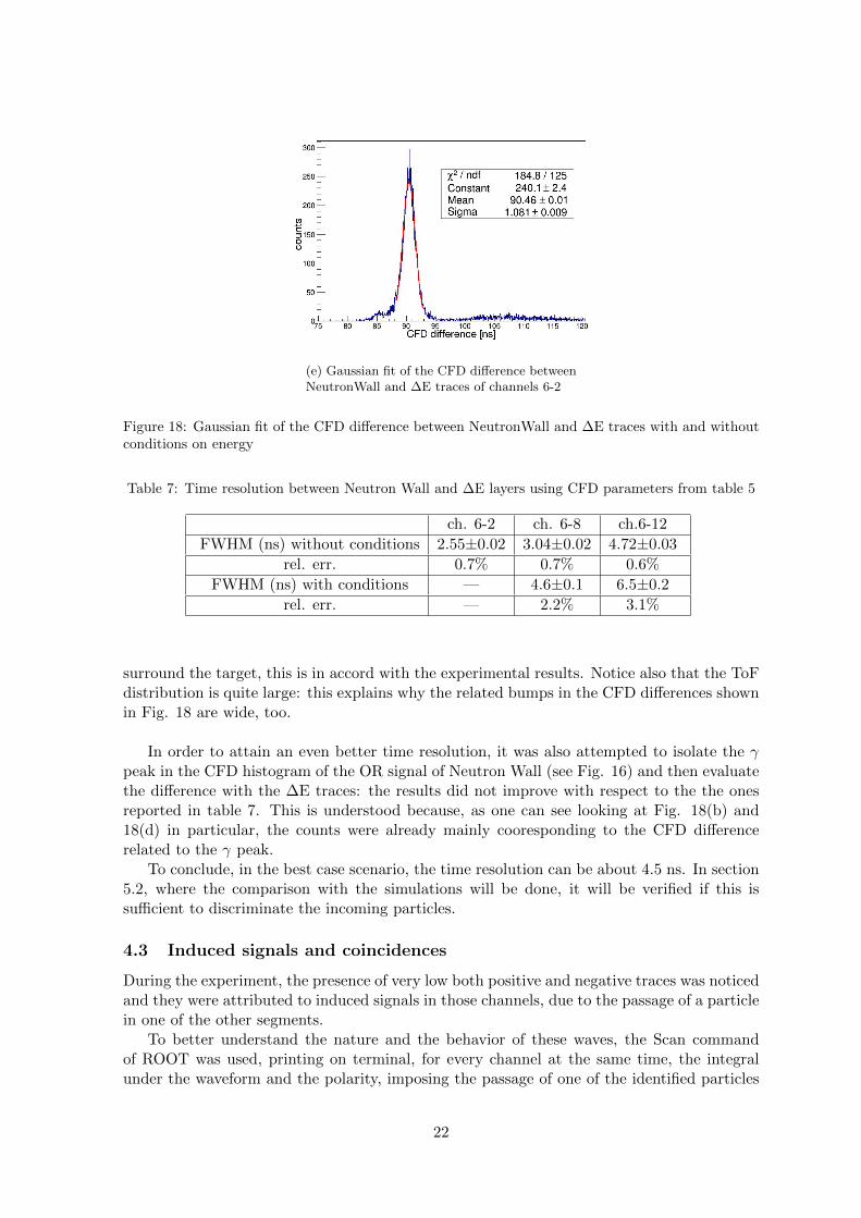
Secondly, the CFD difference between the Neutron Wall and the ∆E channels (usingparameters from table 6) was employed to evaluate the reachable time resolution for theparticles stopping in the ∆E layer. The results are summed up in Fig. 18 and table 7, inwhich two cases are reported:

• without any restriction on the energy of the incident particles (see Fig. 18(a), 18(c)and 18(e));

20

• Setting the energy loss in the E layer equal to 0, to select only the particles stopping inthe first absorber layer, and requesting ∆E<3.72 MeV (which is the maximum energythat protons impinging on the telescope can have to be stopped there, as reported intable 1), in order to get the range in which it is meaningful to distinguish the particles(see Fig. 18(b) and 18(d); for channel 2, it was not possible to have a significantstatistic, since it mostly includes high energy particles).

First of all, note that the CFD difference histogram presents, as expected, a high andquite sharp peak, followed by a small large bump: following the same reasoning previouslydescribed, the peak must be formed by the CFD difference with the OR signals generated bythe γ rays, while the following bump comes from the difference with the traces of neutrons,which present a worse time resolution, compared to γ rays, and less statistic. This is alsoverified by the fact that the temporal difference between the peak and the bump is ∼15-16ns: a simulation of the experiment was run using the COMPA software (see section 5.2 tobetter understand this procedure) to extract the Time of Flight needed by neutrons to getto the Neutron Wall (distant 51 cm from the target) and the result is reported in Fig. 19.The greatest part of neutrons require from 10 to 15 ns to get to the scintillator; consideringthat neutrons are also slowed down by the collisions occurring inside the other detectors that

(a) Gaussian fit of the CFD difference betweenNeutronWall and ∆E traces of channels 6-12

(b) Gaussian fit of the CFD difference betweenNeutronWall and ∆E traces of low energy ofchannels 6-12

(c) Gaussian fit of the CFD difference betweenNeutronWall and ∆E traces of channels 6-8

(d) Gaussian fit of the CFD difference betweenNeutronWall and ∆E traces of low energy ofchannels 6-8

21

(e) Gaussian fit of the CFD difference betweenNeutronWall and ∆E traces of channels 6-2

Figure 18: Gaussian fit of the CFD difference between NeutronWall and ∆E traces with and withoutconditions on energy

Table 7: Time resolution between Neutron Wall and ∆E layers using CFD parameters from table 5

ch. 6-2 ch. 6-8 ch.6-12

FWHM (ns) without conditions 2.55±0.02 3.04±0.02 4.72±0.03

rel. err. 0.7% 0.7% 0.6%

FWHM (ns) with conditions — 4.6±0.1 6.5±0.2

rel. err. — 2.2% 3.1%

surround the target, this is in accord with the experimental results. Notice also that the ToFdistribution is quite large: this explains why the related bumps in the CFD differences shownin Fig. 18 are wide, too.

In order to attain an even better time resolution, it was also attempted to isolate the γpeak in the CFD histogram of the OR signal of Neutron Wall (see Fig. 16) and then evaluatethe difference with the ∆E traces: the results did not improve with respect to the the onesreported in table 7. This is understood because, as one can see looking at Fig. 18(b) and18(d) in particular, the counts were already mainly cooresponding to the CFD differencerelated to the γ peak.

To conclude, in the best case scenario, the time resolution can be about 4.5 ns. In section5.2, where the comparison with the simulations will be done, it will be verified if this issufficient to discriminate the incoming particles.

4.3 Induced signals and coincidences

During the experiment, the presence of very low both positive and negative traces was noticedand they were attributed to induced signals in those channels, due to the passage of a particlein one of the other segments.

To better understand the nature and the behavior of these waves, the Scan commandof ROOT was used, printing on terminal, for every channel at the same time, the integralunder the waveform and the polarity, imposing the passage of one of the identified particles

22

Figure 19: Simulated ToF of neutrons needed to reach the Neutron Wall

in a pair of channels (for example, the response of channels 8-9 and 12-13 to the passage ofa proton in channels 2-3): this was done for every particle in each pair of channels.

The principal observation is that the ∆E channels present, in general, more induced signalsthan the E ones: the reason may be that, since they are thinner, they are more sensitive tosmall variations in charge distribution caused by ions passing near them, even if not through.Another remarkable fact is that the passage of any particle through channels 2 and 3 causeway more induced signals than the passage of the same type of particle through a pair ofthe other channels generates in 2 and 3: this may be related to the issue in the electronicsof these channels previously supposed. The amplitude of the induced waves is very low withrespect to the one of the real particles: referring to Fig. 9, they could be represented bythe points composing the structure in the bottom left of the E-∆E matrices, so values lowerthan ∼20 in ∆E and than ∼40 in E in channel units. Lastly, there is no evident correlationbetween the polarity of the induced signal and the energy or the type of the incident particle,or the channel being crossed, even if, in general, more positive than negative induced signalswere observed.

Again with the Scan command on ROOT, a study on the coincidence of particles wasmade. As expected, most of them involve firstly protons and secondly α, since they constitutethe greatest part of the statistic. Even some events involving 3 different segments at the sametime were spotted.The greater part of coincidences occur between channel 9-8 and 3-2, many between 9-8 and13-12, while only few between 3-2 and 13-12: since an event classified as coincidence can alsobe the passage of the same isotope through 2 different sectors, this is a direct check of therelative positions of the segments to which the digitizer channels are connected, as shown inFig. 20.

Figure 20: Scheme of a telescope divided in segments and the respective connected channels

23

5 Comparisons with the simulations

This section is dedicated to the theoretical check of the results experimentally obtained andthe possibilities that they provide for further and in-depth studies.

5.1 Calibration check

The check on the calibration was accomplished by verifying if the origin of the 3He crossingthe segments (visible, for example, in Fig. 9(b)) is the elastic scattering of the 64Zn beamwith the above-mentioned isotopes implanted inside the W layer.

In order to do that, a simulation of that process was made with the Kinematics Calculatorof LISE++, setting the total beam energy at 250 MeV (3.91 MeV/u), supposing that thereaction takes place in the middle of the target and asking for the kinematics plots at theentrance of the detector. The graph in Fig. 21 shows the energy of the scattered nuclei as afunction of their angle of emission. For the simulation, the telescope connected to channels 9and 8 was considered. It was positioned at an angle of ∼30o with respect to the direction ofthe beam and it was supposed to be square, having a height and a length of 2 cm each: thegreen lines represent both the angular and the energetic ranges interested by the detector. Asone can see, in that region, the incident 3He particle can acquire an energy included between∼8.77 and ∼12.46 MeV/u, that corresponds to

∼ 26.31− 37.38 MeV.

This result has to be compared with the registered energy of the 3He in the experiment,therefore a (E+∆E)-∆E matrix was built (because the theoretically calculated energy is thetotal energy of the particle impinging on the telescope) for channels 9-8 in units of MeV,basing on the conversions reported in table 2. The obtained matrix with the condition onthe 3He is depicted on Fig. 22.

Figure 21: Kinematics plot of the scattering between 64Zn beam and 3He: the range interested by theconsidered detector is delimited by the green lines

As expected, the number of events is much higher in the energy range predicted for theelastic scattering (∼26.31-37.38 MeV), therefore, we are reassured that it actually takes animportant part in the 3He statistic and that the calibration was well done.

Since the evaporation of 3He is very unlikey, it is probable that also the low energy eventswere originated from the scattering between the target and the beam, then slowed down by

24

Figure 22: Experimentally registered energy of the 3He by channels 9-8. The greatest part of theevents occur in the energy range predicted by the simulations for the elastic scattering between thebeam and the target

additional collisions occurring inside the different materials present between the target andthe detectors (such as the backing or other sectors of the detector itself).

5.2 Time of Flight

Finally, we wanted to compare the experimental distribution of the charged-particles Timeof Flight obtained with the NeutronWall and the ∆E layer with a simulated distribution.Indeed in order to determine if the resolution obtained during the experiment is sufficient todiscriminate particles using the ToF, we considered this step as fundamental.

To do that, some Monte Carlo simulations of both the reactions 64Zn −→ 3He and64Zn −→ 16O were accomplished through the COMPA fusion-evaporation reaction code,whose functionalities are described in [6]. In this test, the most realistic situation possiblewas requested:

• the backing of a 179Au 10mg/cm2 thickness, with a density of 19.311 g/cm3, was in-serted, as well as the W support, for a thickness of 0.62 µm;

• it was imposed for both p and α to be slowed down by the collisions happening insidethe target;

• the ASC (Agata Simulation Code) input was generated to have text files containing therelevant information for the particles.

The output of COMPA is a text file, containing the process simulated event-by-event andincludes a number that identifies the evaporated particle, its energy in keV and the directionwhere it is emitted (expressed in Cartesian coordinates, supposing that the beam hits thetarget in the origin of the frame of reference). A C++ program was written to convert theoutput to a ROOT file, containing the energy, the angle of emission (extracted from thedirection vector), the velocity of the particle, and the Time of Flight, i.e. the time that theparticle needs to cover the distance between the target and the EUCLIDES detector, whichis equal to ∼6.5 cm. The ToF was evaluated as

v =

√2E

m−→ ToF =

d

v.

25

The simulations were performed in four different situations:

• 3He target; protons and α detected in the same channel (Fig. 23(a));

• 16O target; protons and α detected in the same channel (Fig. 23(b));

• 3He target; protons and α detected in all possible channels (Fig. 23(c));

• 16O target; protons and α detected in all possible channels (Fig. 23(d)).

(a) Time of Flight differences between α-

particles and protons, setting the 3He target;protons and α detected in the same channel

(b) Time of Flight differences between α-

particles and protons, setting the 16O target;protons and α detected in the same channel

(c) Time of Flight differences between α-

particles and protons, setting the 3He target;protons and α detected in all possible channels

(d) Time of Flight differences between α-

particles and protons, setting the 16O target;protons and α detected in all possible channels

Figure 23: Simulation of Time of Flight differences between α-particles and protons in different cases

In Fig. 23, the Time of Flight differences between α and p are reported, setting a conditionon energy so that it would have been relevant to discriminate the particles stopping in the∆E layer (i.e. 3.72 MeV, which is the maximum energy allowed for protons, as said in table1) and a condition on the difference of angular emission between the two, which was set to5o, in order to avoid to get the ToF difference between a forward and a backward particle.

Accordingly to the energy distribution of the particles, the majority of the events have aToF difference of ∼2-3 ns. This is an unfortunate result, because the attained time resolution,

26

as reported in table 7, is of the same order of magnitude, therefore in most cases it would beimpossible to distinguish the incoming particles among them.

Nevertheless, a plot of the superposition of the Time of Flight distribution of protons(blue) and α particles (red) having an energy inferior to 3.72 MeV when impinging on thetelescope, shows that one can still extract information on the incident particles basing on theTime of Flight, see Fig. 24. Looking at the tails of the histograms, in fact, we deduce thata particle with a ToF greater than ∼15 ns must be an α: this also explain the peaks around27 ns in Fig. 23, which correspond to the difference between very low energy α and ∼3.72MeV protons. Moreover, the fact that, at 3.72 MeV, a proton needs ∼2.4 ns to reach thedetector, while an α requires ∼5 ns, suggests that, even if the ToF difference is about thetime resolution, so individually it does not allow to separate the isotopes, a simultaneous andcombined analysis of the Time of Flight and the energy could permit to attain the desiredresults in future studies.

(a) Superposition of the Time of Flight distri-

butions of p and α with 3He target

(b) Superposition of the Time of Flight distri-

butions of p and α with 16O target

Figure 24: Simulation of Time of Flight of α particles (red) and protons (blue), both impinging onthe telescope having an energy inferior to 4 MeV

27

6 Conclusions

In this work, the capabilities of a Si E-∆E telescope of the light charged-particle detectorEUCLIDES, coupled with the CAEN V1730B 500 MS/s digitizer, were explored. The mainanalysed features of this setup are the energy and the timing performances.

The trapezoidal filter technique was used to stimate the energy, using specifically foundparameters:

k = 285 samples, l = 500 samples, k′ = 5 samples.

This lead to excellent results, in particular for the segments connected to the channels 8 and9. In fact, it has been possible to draw some very precise E-∆E matrices, showing the punch-through of different isotopes. This allowed to calibrate in energy every channel separately.The resulting calibration has finally been verified in section 5.1, where the origin of the 3Heevents and their energy were investigated.

Also the timing has given excellent outcomes: the accurate search for the CFD parameterslead to separate the cases of high energy and low energy particles, resulting in the timeresolutions, between the E and the ∆E layers :

FWHMhigh energy = 1.340± 0.003 ns FWHMlow energy = 4.52± 0.01 ns

The CFD difference between the Neutron Wall and the ∆E channels has also been evalu-ated, since it can be used to determine the time resolution for particles stopped in that siliconlayer. In order to do this, restrictions on the energy range of the incident isotopes were set,so that it was important to be able to discriminate, in particular, α particles from protons.The time resolution obtained under these conditions is:

FWHMstopping particles = 4.6± 0.1 ns

The simulations of the experiment made with COMPA have shown that the Time of Flightdifference between α and protons, having both an energy lower than ∼4 MeV, is most likelyaround 2-3 ns. Therefore, with this time resolution it is not possible to distinguish the in-coming particles among them, at least with this particular reaction and with these energiesinvolved.

To conclude, the pulse shape analysis of the outputs of the CAEN V1730B 500 MS/s dig-itizer connected to a segmented telescope of EUCLIDES has allowed to reach some promisingresults, that can represent a solid base for the future broadening of this technology to the fullstructure of the detector and for more detailed studies, such as a disentanglement based notsolely on the Time of Flight, but also combined with the energy of the particles involved.

Finally, note that, on this work, a brief article [7], reported in this document as attach-ment, has also been written and submitted for publication in the Annual Report 2017 ofLNL.

28

7 References

[1] D. Testov et al., The first physical campaign of the EUCLIDES Si-ball detector coupledto GALILEO gamma-ray spectrometer, LNL-INFN Ann. Rep. 2015.

[2] D. Testov et al., Light charged particle detector EUCLIDES for the GALILEO cam-paign, LNL-INFN Ann. Rep. 2014.

[3] G. F. Knoll, Radiation Detection and Measurements, 4th Edition, John Wiley & SonsInc, 2010.

[4] C. Tintori, Digital Pulse Processing in Nuclear Physics, Rev. 2.1, 2011, fromhttp://www.caen.it/documents/News/20/WP2081 DigitalPulseProcessing Rev 2.1.pdf.

[5] V. T. Jordanov et al., Digital synthesis of the pulse shapes in real time for high resolutionradiation spectroscopy, NIM, A 353 (1994) 261.

[6] J. Mierzejewski et al., The COMPA manual, fromwww.old.slcj.uw.edu.pl/∼jmierz/compa.pdf.

[7] G. Sighinolfi et al., Pulse Shape Analysis of the digitized EUCLIDES signals, LNL-INFNAnn. Rep. 2017.

29

Pulse Shape Analysis of the digitized EUCLIDES signals

G. Sighinolfi1, A. Goasduff1,2, D. Mengoni1,2, M. De Rizzo1, D. Testov1,2, M. Siciliano3, G. Jaworski3,J.J. Valiente-Dobon3

1 Dipartimento di Fisica e Atronomia dell’Universita di Padova, Padova, Italy.2 INFN, Sezione di Padova, Padova, Italy.

3INFN, Laboratori Nazionali di Legnaro, Legnaro (Padova), Italy.

INTRODUCTION

EUCLIDES [1] is a silicon-ball detector of light chargedparticles, used as an ancillary device of the γ-rayspectrometer GALILEO at LNL [2]. It consists of 55∆E-E telescopes of hexagonal and pentagonal shapes, whosethicknesses are ∼130 and ∼1000 µm for ∆E and E layers,respectively, and whose surfaces are ∼10 cm2 each. Thecomplete structure has a diameter of nearly 13 cm and asolid angle coverage close to 4π. Due to the kinematicsenlargement of the solid angle in the center of mass referenceframe for a typical fusion-evaporation reaction (v/c≈5%),the most forward positioned telescopes have to deal withhigher counting rates with respect to the others. Thusthe 5 most forward detectors are segmented in 4 equalparts, which have individual electronic processing circuits,to reduce the probability of pile-up.

In December 2017, the EUCLIDES array was used inan experiment, during which a 250 MeV 64Zn beam wasimpinging on a 3He target, implanted in a W layer depositedon a thick Au backing. A CAEN V1730B, which is a 1-unitwide VME module housing 16 channels 14-bit 500 MS/sFlash ADC Waveform digitizer, was employed to readout3 segments of one of the most forward telescopes. 3 evenchannels were connected to the ∆E layers and 3 odd ones tothe E. An additional channel was connected to the OR signalof the Neutron Wall array [3].

The aim of the implementation of this device in theread-out chain of EUCLIDES is to have the possibilityto disentangle α and protons stopping in the ∆E layer.Depending on the kinematics of the reaction and thethickness of the absorber layers, used to prevent the elasticscattering of the beam (target) from reaching the detectors,those events stopping in the ∆E can represent more than 50%of the detected particles. In order to reach the maximumparticle detection efficiency and selectivity in the lightcharged particle-γ-rays in fusion-evaporation reaction, newmethods of particle discrimination have been investigatedfor the EUCLIDES array.

EXPERIMENTAL RESULTS

An example of the traces as recorded online by the digitizerduring the experiment is presented in Fig. 1. The verticallines close to 1.25 and 1.5 µs correspond to the OR

trigger coming from the Neutron Wall array, which, inthis experiment, presents the advantage of being a highefficiency γ-ray detector with a fast response. Due to thelarge counting rate on this channel (∼ 400 kHz), the choicewas made to use it only in coincidence with the E and ∆Esignals. The polarity of the waveforms was set negativein the digitizer options and the leading edge threshold wasadjusted individually for each channel. As expected, theamplitude of the signals coming from odd channels is largerthan the one of even channels, since the first are connectedto E segments, in which the energy loss is higher.

Fig. 1. Online digitized signals from the EUCLIDES segmenteddetectors read with the CAEN V1730B module during an in-beamexperiment. The OR trigger of Neutron Wall and the waveforms ofa ∆E and a E channels are visible.

An offline analysis was performed on the digitized signalsin order to extract the energy in both E and ∆E layers.Combining the two, the E-∆E identification matrix, seeFig. 2, was contructed. One can clearly idetify p, d, 3He andα, with some additional structures attributable to t and 2p(or pile-up of protons). Thanks to the clear punch-throughof p, d and α, the energy calibrations of the two layers wereevaluated. The energies have been extracted by applyinga trapezoidal filter following the equations established byJordanov et al. in [4] on all the traces overcoming a softwarethreshold. This second threshold has been implemented toreduce the processing time, because the CAEN digitizer issampling all the active channels and dumping them to diskas soon as one of them is overcoming the hardware triggerthreshold.

To identify the particles stopping in the ∆E layer, weexplore, in this contribution, the discrimination based solely

30

Fig. 2. The E-∆E matrix obtained after the trapezoidal filteringof the recorded traces for one telescope. The amplitude ofthe signal extracted in both layers has been calibrated using thepunch-through of the light particles.

on the time-of-flight (ToF). Thus a large effort has beendedicated in the optimization of the time resolution basedon the difference between two CFD signals. During apreliminary test, the timing performances of the digitizerhave been studied through the measurement of the CFDdifference between a ∼1 V signal coming from a waveformgenerator and the same delayed by 16 ns. In this case, anaccurate search of the optimal CFD parameters has beenachieved through the trial of many different combinationsof fraction and delay, looking for the ones giving the lowestpossible value of σ for the gaussian fit of the CFD differencebetween the two. With fraction of 42% and delay of 58samples, the reached result is FWHM = 50.4±0.2 ps.

Considering the experimental data, the best resolution wasobtained with two distinct sets of parameters for the analysis:one for high energy particles, which require smaller valuesof fraction and delay, and the other for particles at lowenergy, which need higher ones to overcome the CFDthreshold. The first set of parameters leads to a timeresolution of ∼1.3 ns between the moment in which theparticle hits the ∆E layer and when it hits the E one, while,using the other set, one can get a time resolution of ∼4.5 ns.

To evaluate the ToF of particles stopping in the ∆E layer,the logical OR signal of the Neutron Wall was employed.Since a logical signal was used, it should give a very accurateCFD position and provide a precise time resolution whendoing the difference with the CFD of the ∆E traces of theother channels. Setting conditions in order to select onlythe particles that stop in the first layer and have an energyinferior to 4 MeV, the time resolution is 4.6±0.1 ns, seeFig. 3. Notice that the structure of these CFD differencespresents a sharp peak, related to the γ-rays signals in NeutronWall, followed by a smaller bump, which is instead due tothe detection of neutrons.

To understand if this time resolution is sufficient tohave the possibility to distinguish α particles from protonsstopping in the ∆E layer, a numerical test was made with theCOMPA fusion-evaporation reaction code [5], simulating

the experiment of interest. The result shows that the ToFdifference between α and p to cover the distance separatingthe detector from the target, at a low enough energy to avoidthe punch-through of ∆E, is most likely between 2 and 3ns. It means that the ToF is too small to allow the particlesdiscrimination based only on the method explained above, atleast with this specific reaction and these energies involved.Possible improvements may be obtained through a combinedanalysis of the ToF and the energy.

Fig. 3. Time resolution based on digital CFD algorithm applied onNeutron Wall’s OR signals and ∆E traces.

CONCLUSIONS

The first experimental results of the implementation of a500 MS/s digitizer in the read-out chain of an EUCLIDESsegmented detector are reported. The offline PulseShape analysis provides promising results: the E-∆Ematrix, obtainable through trapezoidal filter, shows aclear identification of the different isotopes; a good timeresolution of ∼1.3-4.5 ns between the E and ∆E layer hasbeen obtained. On the other hand, a discrimination basedsolely on the ToF does not permit to distinguish α particlesfrom protons stopping in the first layer of the detector, atleast in this particular experiment: the time resolution of theCFD difference between the Neutron Wall and the ∆E tracesof interested particles (esteemed to be ∼4.5 ns) is of thesame order of magnitude as the ToF difference between theseparticles in the previously described experimental conditions(∼2-3 ns).

[1] D. Testov et al., LNL-INFN Ann. Rep. (2015), 105 .[2] J.J. Valiente-Dobon et al., LNL-INFN Ann. Rep. (2014), 95 .[3] O. Skeppstedt et al., NIM, A 421 (1999), 531.[4] V. T. Jordanov et al., NIM, A 353 (1994) 261.[5] J. Mierzejewski et al., The COMPA manual, from

www.old.slcj.uw.edu.pl/∼jmierz/compa.pdf.

31