Universidade Federal de Minas Gerais, Belo Horizonte/MG ... · Artur J. Lemonte Departamento de Estat´ıstica, CCET Universidade Federal do Rio Grande no Norte, Natal/RN, Brazil

BJPS -A

ccep

ted M

anusc

ript

On the Nielsen distribution

Fredy CastellaresDepartamento de Estatıstica, ICEX

Universidade Federal de Minas Gerais, Belo Horizonte/MG, Brazil

email: [email protected]

Artur J. LemonteDepartamento de Estatıstica, CCET

Universidade Federal do Rio Grande no Norte, Natal/RN, Brazil


Marcos A.C. SantosDepartamento de Estatıstica, ICEX

Universidade Federal de Minas Gerais, Belo Horizonte/MG, Brazil


Abstract

We introduce a two-parameter discrete distribution that may have a zero vertex and can beuseful for modeling overdispersion. The discrete Nielsen distribution generalizes the Fisher log-arithmic (i.e. logarithmic series) and Stirling type I distributions in the sense that both can beconsidered displacements of the Nielsen distribution. We provide a comprehensive account of thestructural properties of the new discrete distribution. We also show that the Nielsen distributionis infinitely divisible. We discuss maximum likelihood estimation of the model parameters andprovide a simple method to find them numerically. The usefulness of the proposed distribution isillustrated by means of three real data sets to prove its versatility in practical applications.

Keywords: Discrete distribution; Fisher logarithmic distribution; Nielsen expansion; Stirling dis-tributions.

1 Introduction

Count data occur in many practical problems as, for example, the number of occurrences of thunder-storms in a calendar year, the number of accidents, the number of absences, the number of days lost,

1

BJPS -A

ccep

ted M

anusc

ript

the number of insurance claims, the number of kinds of species in ecology, and so on. Discrete dis-tributions, which describe count phenomena, have been proposed in the statistical literature in recentyears, due perhaps to advances in computational methods which enable us to compute, straightfor-wardly, the numerical value of special functions such as hypergeometric series. To mention a few, butnot limited to, the readers are referred to Roy (2004), Inusah and Kozubowski (2006), Kozubowskiand Inusah (2006), Krishna and Pundir (2009), Jazi et al. (2010), Nooghabi et al. (2011), Englehardtand Li (2011), Nekoukhou et al. (2013), Barbiero (2014), among many others.

It is well-known that the classical Poisson distribution is applied in many scientific fields involv-ing count data, mainly because of its simplicity. As pointed out by Gomes-Denis et al. (2011), mostfrequencies of event occurrence can be described initially by a Poisson distribution. However, a ma-jor drawback of this distribution is the fact that the variance is restricted to be equal to the mean, asituation that may not be consistent with observation. So, alternative discrete probability distribu-tions, such as the negative binomial distribution, are preferred for modeling the phenomena understudy. Additionally, many of these phenomena, such as individual automobile insurance claims, arecharacterized by two features: (i) overdispersion, that is, the variance is greater than the mean; (ii)zero-inflated (or zero vertex), that is, the presence of a high percentage of zero values in the empiricaldistribution. In view of this, many attempts have been made in the statistical literature to propose newdiscrete family of distributions for the distribution of the number of counts.

It is worth emphasizing that the majority of the new discrete distributions proposed recently in thestatistical literature are obtained by discretizing a known continuous distribution (see the above refer-ences). Instead, we will introduce a new two-parameter discrete distribution on the basis of a seriesexpansion presented in Nielsen (1906). As we will see latter, the new distribution is very simple todeal with, since its probability mass function does not contain any complicated function. Further, it isvery flexible and it also presents the twofold characteristic stated above: it can have a zero vertex, andit is overdispersed. Therefore, it may be a natural candidate for fitting phenomena of this nature. Thereal data examples provided here, and the comparison with the Negative Binomial (NB) distribution(the most important and popular two-parameter discrete distribution for overdispersed data), showthat the proposed distribution has an outstanding performance. In addition to the NB distribution, wealso consider the Zero-Inflated Poisson (ZIP) and Zero-Inflated NB (ZINB) distributions in the realdata applications for the sake of comparison.

The main aim of this paper is to introduce a new two-parameter discrete family of distributionswith the hope that the new distribution may have a ‘better fit’ compared to the NB distribution (andother ones) in certain practical situations. Additionally, we will provide a comprehensive account ofthe mathematical properties of the proposed new family of distributions. As we will see later, theformulas related with the new distribution are simple and manageable, and with the use of moderncomputer resources and its numerical capabilities, the proposed distribution may prove to be an usefuladdition to the arsenal of applied statisticians in discrete data analysis.

In order to introduce the new discrete distribution, we consider the following series expansion

2

BJPS -A

ccep

ted M

anusc

ript

provided by Nielsen (1906)[− log(1− z)

z

]α= 1 + α z

∞∑n=0

ψn(n+ α)zn, α ∈ R, |z| < 1, (1)

where the coefficients ψn(·) are Stirling polynomials. According to Ward (1934), these coefficientscan be expressed in the form

ψn−1(w) =(−1)n−1

(n+ 1)!

[Hn−1

n − w + 2

n+ 2Hn−2

n +(w + 2)(w + 3)

(n+ 2)(n+ 3)Hn−3

n − · · ·

+ (−1)n−1 (w + 2)(w + 3) · · · (w + n)

(n+ 2)(n+ 3) · · · (2n)H0

n

],

(2)

where Hmn are positive integers defined recursively by Hm

n+1 = (2n+1−m)Hmn +(n−m+1)Hm−1

n ,withH0

0 = 1,H0n+1 = 1×3×5×· · ·×(2n+1),Hn

n+1 = 1. The first six polynomials are ψ0(w) = 1/2,ψ1(w) = (2+3w)/24, ψ2(w) = (w+w2)/48, ψ3(w) = (−8− 10w+15w2+15w3)/5760, ψ4(w) =

(−6w − 7w2 + 2w3 + 3w4)/11520 and ψ5(w) = (96 + 140w − 224w2 − 315w3 + 63w5)/2903040.We would like to point out that according to another definition1, the polynomials S0(w) = 1 and

Sn(w) = n!(w + 1)ψn−1(w), for n ≥ 1, are also known as Stirling polynomials. In this paper, weuse this terminology to refer to the polynomials ψn(w) in accordance with Nielsen (1906) and Ward(1934).

We have the following propositions.

Proposition 1. The expansion (1) is absolutely convergent.

Proof. The proof can be found in Flajonet and Sedgewick (2009, p. 385).

Proposition 2. The expansion (1) can be rewritten as

1 =zα

[− log(1− z)]α

∞∑m=0

ρm(α)zm, 0 < z < 1, (3)

where ρ0(α) = 1 and ρm(α) = αψm−1(α +m− 1) for m ≥ 1.

Proof. We can express[− log(1− z)

z

]α= 1 + α

∞∑n=1

ψn−1(n− 1 + α)zn =∞∑n=0

ρn(α)zn,

where ρ0(α) = 1, and ρn(α) = αψn−1(α + n− 1) for n ≥ 1. It then follows that

1 =zα

[− log(1− z)]α

∞∑m=0

ρm(α)zm, 0 < z < 1.

1See, for example, http://mathworld.wolfram.com/StirlingPolynomial.html

3

BJPS -A

ccep

ted M

anusc

ript

Proposition 3. The coefficients ρm(α) in (3) satisfy

ρm(α) = αψm−1(m+ α− 1) > 0,

for m ≥ 1 and α > 0.

Proof. In order to proof that ψm−1(m + α − 1) > 0 for m ≥ 1 and α > 0, we shall use therepresentation of Stirling polynomials given by Graham et al. (1994). The Nielsen expansion in (1)can be rewritten as[

− log(1− z)

z

]α= 1 + α

∞∑n=1

σn(n+ α)zn, α > 0, |z| < 1,

where the polynomials σn(·) are defined as (Graham et al., 1994)

σn(n+ α) =

∑n−1k=0

⟨⟨nk

⟩⟩ (n+k+α

2n

)α(α + 1) · · · (α + n)

.

Here,⟨⟨

nk

⟩⟩are the Eulerian numbers of the second kind, which satisfy the recurrence relation⟨⟨ n

m

⟩⟩= (2n−m− 1)

⟨⟨n− 1

m− 1

⟩⟩+ (m+ 1)

⟨⟨n− 1

m

⟩⟩, n,m ∈ N,

with initial condition ⟨⟨0

0

⟩⟩= 1,

⟨⟨0

m

⟩⟩= 1, m = 0.

The Eulerian numbers of the second kind are not negative (Graham et al., 1994, p. 271). Fromdefinition of σn(α + n), we have that σn(α + n) > 0 for all α > 0 and n ∈ N. Hence, by noting that

ψn−1(n+ α− 1) = σn(n+ α) > 0, n ≥ 1, ∀ α > 0,

the result holds.

The rest of this paper is organized as follows. In Section 2 we introduce the new discrete distri-bution. Structural properties related to the new distribution are provided in Section 3. Estimation ofmodel parameters is discussed in Section 4. Section 5 deals with applications to real data sets. TheSection 6 ends up the paper with some final comments.

2 The new discrete distribution

By considering Propositions 2 and 3, we define the two-parameter discrete distribution named as thediscrete Nielsen (‘dN’ for short) distribution. We have the following definition.

4

BJPS -A

ccep

ted M

anusc

ript

Definition 1. The probability mass function of X with dN distribution is given by

Pr(X = x) =pθ+x ρx(θ)

[− log(1− p)]θ, x = 0, 1, 2, . . . , (4)

where p ∈ (0, 1), θ > 0, ρ0(θ) = 1,

ρx(θ) = θ ψx−1(θ + x− 1), x = 1, 2, . . . ,

and the coefficients ψx(·) are the Stirling polynomials given in (2).

If X follows a dN distribution, then the notation used is X ∼ dN(p, θ). The dN probability massfunction in (4) is very simple and does not involve any complicated function. Additionally, there isno functional relationship between the parameters p ∈ (0, 1) and θ > 0, and they vary freely in theparameter space. We have that

Pr(X = 0) =pθ

[− log(1− p)]θ, Pr(X = 1) =

θ pθ+1

2 [− log(1− p)]θ,

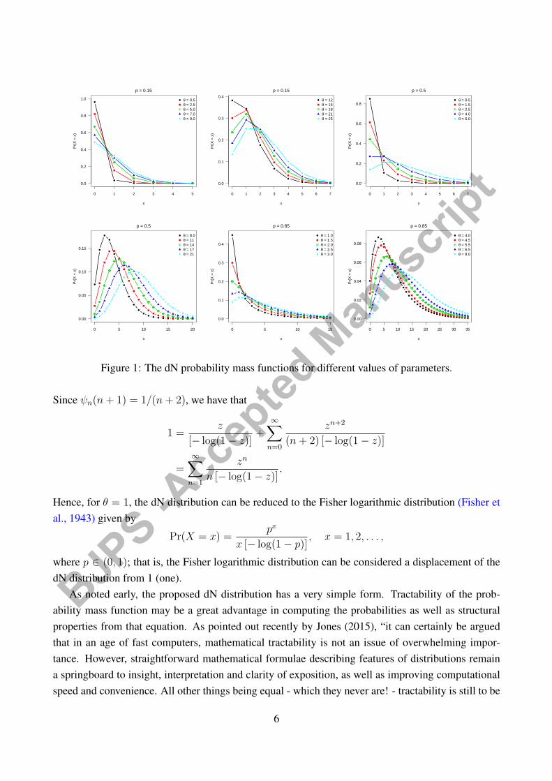
and the other probabilities can be easily computed. For fixed p ∈ (0, 1), it follows that Pr(X = 0) →1 as θ → 0+, which means that the dN model can have a zero vertex. However, all zeros must beinterpreted as observational zeros from the dN distribution, that is, the proposed dN model does notact a zero-inflated model. Figure 1 displays some possible shapes of the dN probability mass functiongiven by expression (4). Note that the mode moves away from zero with increasing θ, for p fixed,indicating that the new discrete distribution is very versatile.

From Nielsen expansion (1) and when α = 1, it follows that[− log(1− z)

z

]= 1 + z

∞∑n=0

ψn(n+ 1)zn, 0 < z < 1.

Additionally, we have that

− log(1− z) = z +z2

2+z3

3+ · · · , 0 < z < 1.

After some algebra, we obtain[− log(1− z)

z

]= 1 +

z

2+z2

3+ · · ·

= 1 + z

[1

2+z

3+ · · ·

]= 1 + z

∞∑n=0

zn

n+ 2.

5

BJPS -A

ccep

ted M

anusc

ript0 1 2 3 4 5

0.0

0.2

0.4

0.6

0.8

1.0

x

Pr(

X =

x)

θ = 0.5θ = 2.5θ = 5.0θ = 7.0θ = 9.0

p = 0.15

0 1 2 3 4 5 6 7

0.0

0.1

0.2

0.3

0.4

x

Pr(

X =

x)

θ = 12θ = 15θ = 18θ = 21θ = 25

p = 0.15

0 1 2 3 4 5 6 7

0.0

0.2

0.4

0.6

0.8

x

Pr(

X =

x)

θ = 0.5θ = 1.5θ = 2.5θ = 4.0θ = 6.0

p = 0.5

0 5 10 15 20

0.00

0.05

0.10

0.15

x

Pr(

X =

x)

θ = 8.0θ = 11θ = 14θ = 17θ = 21

p = 0.5

0 5 10 15

0.0

0.1

0.2

0.3

0.4

x

Pr(

X =

x)

θ = 1.0θ = 1.5θ = 2.0θ = 2.5θ = 3.0

p = 0.85

0 5 10 15 20 25 30 35

0.00

0.02

0.04

0.06

0.08

x

Pr(

X =

x)

θ = 4.0θ = 4.5θ = 5.5θ = 6.5θ = 8.0

p = 0.85

Figure 1: The dN probability mass functions for different values of parameters.

Since ψn(n+ 1) = 1/(n+ 2), we have that

1 =z

[− log(1− z)]+

∞∑n=0

zn+2

(n+ 2) [− log(1− z)]

=∞∑n=1

zn

n [− log(1− z)].

Hence, for θ = 1, the dN distribution can be reduced to the Fisher logarithmic distribution (Fisher etal., 1943) given by

Pr(X = x) =px

x [− log(1− p)], x = 1, 2, . . . ,

where p ∈ (0, 1); that is, the Fisher logarithmic distribution can be considered a displacement of thedN distribution from 1 (one).

As noted early, the proposed dN distribution has a very simple form. Tractability of the prob-ability mass function may be a great advantage in computing the probabilities as well as structuralproperties from that equation. As pointed out recently by Jones (2015), “it can certainly be arguedthat in an age of fast computers, mathematical tractability is not an issue of overwhelming impor-tance. However, straightforward mathematical formulae describing features of distributions remaina springboard to insight, interpretation and clarity of exposition, as well as improving computationalspeed and convenience. All other things being equal - which they never are! - tractability is still to be

6

BJPS -A

ccep

ted M

anusc

ript

preferred to non-tractability.” In view of this, the tractability of the two-parameter dN distribution isvery welcome and, as a consequence, all properties derived in the next section (Section 3) have verysimple forms. Again, as pointed out recently by Jones (2015), “the role of parsimony in statisticalmodelling, to aid interpretation (that word again!), to facilitate estimation and particularly prediction,affording generalisability of results by avoiding overfitting, is clear. In developing families of distri-butions, however, the watchword has usually been flexibility, and parsimony is little mentioned.” Wehave that the dN distribution has only two parameters (p ∈ (0, 1) and θ > 0) which has facilitated theestimation of these parameters by the maximum likelihood method (see Section 4). In short, we haveproposed a very simple discrete distribution with only two parameters and which is very flexible.

3 Properties

In what follows, we study several structural properties of the two-parameter dN distribution. We havethe following propositions.

Proposition 4. Let X ∼ dN(p, θ). Then, the probability generating function is

GX(s) = E(sX) =[log(1− ps)

s log(1− p)

]θ, 0 < s <

1

p, θ = 1.

For θ = 1, it follows that

GX(s) = E(sX) =log(1− ps)

log(1− p), 0 < s <

1

p.

Proof. For θ = 1, we have that

GX(s) = E(sX) =∞∑x=0

sxpθ+x ρx(θ)

[− log(1− p)]θ.

After some algebra, we obtain

GX(s) =

[log(1− ps)

s log(1− p)

]θ ∞∑x=0

(sp)x+θ ρx(θ)

[− log(1− sp)]θ

=

[log(1− ps)

s log(1− p)

]θ,

where∞∑x=0

(sp)x+θ ρx(θ)

[− log(1− sp)]θ= 1, 0 < s <

1

p.

7

BJPS -A

ccep

ted M

anusc

ript

For θ = 1, we have that

GX(s) = E(sX) =∞∑x=1

sxpx

x[− log(1− p)]

=log(1− ps)

log(1− p)

∞∑x=1

(sp)x

x[− log(1− sp)]

=log(1− ps)

log(1− p),

where∞∑x=1

(sp)x

x[− log(1− sp)]= 1, 0 < s <

1

p.

Proposition 5. Let X ∼ dN(p, θ). Then, the moment generating function is

MX(t) = E(etX) = e−θ t

[log(1− p et)

log(1− p)

]θ, t < − log(p), θ = 1.


MX(t) = E(etX) =log(1− p et)

log(1− p), t < − log(p).

Proof. For θ = 1, we have that

MX(t) = E(etX) =∞∑x=0

etxpθ+x ρx(θ)

[− log(1− p)]θ.


MX(t) =

[log(1− p et)

et log(1− p)

]θ ∞∑x=0

(p et)x+θ ρx(θ)

[− log(1− p et)]θ

= e−θt

[log(1− p et)

log(1− p)

]θ,

where∞∑x=0

(p et)x+θ ρx(θ)

[− log(1− p et)]θ= 1, t < − log(p).

For θ = 1, we have

MX(t) = E(etX) =∞∑x=1

etxpx

x[− log(1− p)]

=log(1− p et)

log(1− p)

∞∑x=1

(p et)x

x[− log(1− p et)]

=log(1− p et)

log(1− p),

8

BJPS -A

ccep

ted M

anusc

ript

where∞∑x=1

(p et)x

x[− log(1− p et)]= 1, t < − log(p).

Proposition 6. Let X ∼ dN(p, θ). Then, the cumulant generating function is

KX(t) = log[MX(t)] = −θ t+ θ{log[− log(1− p et)]− log[− log(1− p)]},

where t < − log(p) and θ = 1. For θ = 1, it follows that

KX(t) = log[MX(t)] = log[− log(1− p et)]− log[− log(1− p)],

where t < − log(p).

Proof. The result follows directly from Proposition 5.

Proposition 7. Let X ∼ dN(p, θ). Then, the characteristic function is given by

ϕX(t) = E(eitX) = e−iθt

[log(1− p eit)

log(1− p)

]θ, t ∈ R, θ = 1.


ϕX(t) = E(eitX) =log(1− p eit)

log(1− p), t ∈ R.

where i =√−1 is the imaginary number.

Proof. The proof is similar to that of Proposition 5 just considering the logarithm function for com-plex variables.

It follows from Proposition 5 that the ordinary moments of X ∼ dN(p, θ), for θ = 1, are given by

µ′r = E(Xr) =

{dr

dtre−θ t

[log(1− p et)

log(1− p)

]θ}t=0

.

For example, the mean (i.e. µ′1) and variance are

E(X) = θ

(p

(1− p) [− log(1− p)]− 1

),

VAR(X) = θp [− log(1− p)− p]

[(1− p) log(1− p)]2.

We have that the mean and variance increase as the values of p ∈ (0, 1) and θ > 0 increase. Table 1lists the values of the mean and variance with varying values of p and θ. The skewness and kurtosis ofX can be calculated from the ordinary moments using well-known relationships. Figure 2 shows how

9

BJPS -A

ccep

ted M

anusc

ript

Table 1: Mean (above) and variance (below) of the dN distribution.θ \ p 0.1 0.3 0.5 0.7 0.90.2 0.011 0.040 0.089 0.188 0.582

0.012 0.055 0.161 0.541 4.7620.5 0.027 0.101 0.221 0.469 1.454

0.030 0.136 0.402 1.352 11.9040.8 0.044 0.161 0.354 0.750 2.327

0.048 0.218 0.643 2.163 19.0471.2 0.065 0.242 0.531 1.126 3.490

0.072 0.327 0.965 3.245 28.5711.6 0.087 0.323 0.708 1.501 4.654

0.095 0.436 1.286 4.327 38.0942.5 0.136 0.504 1.107 2.345 7.272

0.149 0.682 2.010 6.760 59.5224.0 0.218 0.806 1.771 3.752 11.635

0.238 1.091 3.216 10.817 95.236

p theta

Skew

ness

(a)

p

theta

Kurtosis

(b)

Figure 2: Skewness (a) and kurtosis (b) of the dN distribution as functions of p and θ.

10

BJPS -A

ccep

ted M

anusc

ript

these measures vary with respect to p and θ. Note that the skewness and kurtosis of the dN distributioncan be quite pronounced, and the values of both measures decrease as the values of p ∈ (0, 1) andθ > 0 increase.

The index of dispersion (a normalized measure of the dispersion of a probability distribution) ofthe dN distribution, defined as Id = VAR(X)/E(X), takes the form

Id =p [− log(1− p)− p]

[(1− p) log(1− p)]2

(p

(1− p) [− log(1− p)]− 1

)−1

,

which is independent of the parameter θ. It follows that Id > 1 for p ∈ (0, 1), and limp→0+ Id = 1

and limp→1− Id = ∞, which implies that the dN distribution is suitable for modeling count data withoverdispersion, like the NB distribution.

Proposition 8. Let X1 ∼ dN(p, θ1) and X2 ∼ dN(p, θ2) be two independent random variables.Define Z = X1 +X2. The probability mass function (convolution) of Z is given by

Pr(Z = z) =pθ1+θ2+zρz(θ1 + θ2)

[− log(1− p)]θ1+θ2, z = 0, 1, 2, . . . ,

where p ∈ (0, 1), θ1 > 0 (with θ1 = 1), θ2 > 0 (with θ2 = 1), ρ0(θ1 + θ2) = 1, and

ρz(θ1 + θ2) = (θ1 + θ2)ψz−1(θ1 + θ2 + z − 1), z = 1, 2, . . . .

For θ1 = θ2 = 1, we have that

Pr(Z = z) =2! pz

z! [− log(1− p)]2

⌊z2

⌋, z = 2, 3, . . . ,

where⌊nk

⌋(for n ∈ N and k ∈ N) are Stirling numbers of the first kind, and they can be calculated

by the recurrence relation ⌊n+ 1

k

⌋= n

⌊nk

⌋+

⌊n

k − 1

⌋,

with the initial conditions ⌊0

0

⌋= 1,

⌊n0

⌋=

⌊0

n

⌋= 0.

Proof. By using Pr(Z = z) =∑z

x=0 Pr(X1 = x) Pr(X2 = z − x) for θ1 = 1 and θ2 = 1, we obtain

Pr(Z = z) =z∑

x=0

[p

[− log(1− p)]

]θ1px ρx(θ1)

[p

[− log(1− p)]

]θ2pz−x ρz−x(θ2),

After some algebra, we have

Pr(Z = z) =

[p

[− log(1− p)]

]θ1+θ2

pzz∑

x=0

ρx(θ1) ρz−x(θ2).

11

BJPS -A

ccep

ted M

anusc

ript

The convolution of Stirling polynomials has the form (Graham et al., 1994, Cap. 6)

n∑k=0

r σk(k + r) s σn−k(s+ [n− k]) = (r + s)σn(n+ [r + s]).

From this expression we have

z∑x=0

θ1 σx(x+ θ1) θ2 σz−x(θ2 + [z − x]) = (θ1 + θ2)σz(z + [θ1 + θ2]) = ρz(θ1 + θ2),

by using ρ0(α) =: ασ0(α) = 1, and ρx(α) = αψx−1(α + x − 1) = ασx(x + α) with α > 0 andx = 1, 2, . . .. Hence, it follows that

Pr(Z = z) =

[p

[− log(1− p)]

]θ1+θ2

ρz(θ1 + θ2) pz, z = 0, 1, 2, . . . .

For θ1 = θ2 = 1, we have that

Pr(Z = z) =z∑

x=0

[1

[− log(1− p)]

]px

x

[1

[− log(1− p)]

]pz−x

(z − x).


Pr(Z = z) =

[1

[− log(1− p)]

]2pz

z

z−1∑x=1

z

x(z − x)

=

[1

[− log(1− p)]

]2pz

2

z

z−1∑x=1

1

x.

The n-th partial sum of the divergent harmonic series, given by

Mn =n∑

k=1

1

k,

is called the n-th harmonic number. We have that⌊n2

⌋= (n− 1)!Mn−1,

and hence2

z

z−1∑x=1

1

x=

2!

z!(z − 1)!Mz−1 =

2!

z!

⌊n2

⌋.

From the above expression we obtain

Pr(Z = z) =

[1

[− log(1− p)]

]22!

z!

⌊z2

⌋pz, z = 2, 3, 4 . . . ,

which concludes the proof.

12

BJPS -A

ccep

ted M

anusc

ript

The generalization of Proposition 8 is provided in the following proposition.

Proposition 9. Let X1, X2, . . . , Xn be n independent random variables, where Xk ∼ dN(p, θk) fork = 1, 2, . . . , n. Define Z = X1 + · · ·+Xn. If θk = 1 for k = 1, 2, . . . , n, then

Z ∼ dN(p, θ1 + · · ·+ θn).

If θk = 1 for k = 1, 2, . . . , n, then

Pr(Z = z) =pz

[− log(1− p)]nn!

z!

⌊ zn

⌋, z = n, n+ 1, n+ 2, . . . .

Proof. The case θk = 1 for k = 1, 2, . . . , n can be found in Patil (1963). If θk = 1 for k = 1, . . . , n,we consider the inversion theorem (Feller, 1971, p. 511). The characteristic function of Z is given by

ϕZ(t) = E(eitZ) =n∏

k=1

ϕXk(t).

Additionally, we have that

ϕXk(t) = E(eitXk) = e−itθk

[log(1− p eit)

log(1− p)

]θk, t ∈ R, θk = 1,

and hence we obtain

ϕZ(t) =

[p

log(1− p)

]θ1+···+θn[ log(1− p eit)

p eit

]θ1+···+θn

.

Let θ = θ1 + · · ·+ θn. We have

ϕZ(t) =

[p

log(1− p)

]θ ∞∑m=0

ρm(θ) pm eitm, 0 < p < 1.

By using the inversion theorem, there exists a probability function of the form

Pr(Z = z) =1

2π

∫ π

−π

ϕZ(t) e−izt dt,

which is given by

Pr(Z = z) =

[p

log(1− p)

]θ ∞∑m=0

ρm(θ) pm 1

2π

∫ π

−π

ei(m−z)t dt,

where1

2π

∫ π

−π

ei(m−z)t dt =

{1, m = z,

0, m = z.

Hence, it follows that

Pr(Z = z) =

[p

log(1− p)

]θρz(θ) p

z, z = 0, 1, . . . ,


13

BJPS -A

ccep

ted M

anusc

ript

Proposition 10. Let X ∼ dN(p, θ), where p ∈ (0, 1) and θ = n ∈ N. Then, the probability massfunction of X takes the form

Pr(X = x) =pn+x

[− log(1− p)]nn!

(n+ x)!

⌊x+ n

n

⌋, x = 0, 1, 2, . . . . (5)

Proof. From Graham et al. (1994, Cap. 7), we have that[− log(1− p)

p

]n= 1 +

∞∑x=1

n!

(n+ x)!

⌊x+ n

n

⌋px.

Additionally, for x = 0, 1, 2, . . . and n = 1, 2, . . ., it follows that

ψx(x+ n) =(n− 1)!

(n+ 1 + x)!

⌊n+ 1 + x

n

⌋,

which completes the proof.

Let Z be a random variable with probability mass function given by

Pr(Z = z) =pz

[− log(1− p)]nn!

z!

⌊ zn

⌋, z = n, n+ 1, n+ 2, . . . .

We will name the above distribution as the discrete Stirling type I (‘dS’ for short) distribution withparameters p ∈ (0, 1) and n ∈ N, say Z ∼ dS(p, n). The dS distribution appeared for the first timein Patil (1963) as a convolution of n random variables with Fisher logarithmic distribution; see alsoPatil and Wani (1965). We have the following proposition.

Proposition 11. Let X ∼ dN(p, n) and Z ∼ dS(p, n), where n ∈ N and 0 < p < 1. Then, thedS distribution is a displacement of the dN distribution from n ∈ N and, additionally, is fulfilledZ = X + n.

Proof. The proof follows from equation (5) and by defining Z = X + n.

Finally, we have the following proposition.

Proposition 12. Let X ∼ dN(p, θ), where p ∈ (0, 1) and θ > 0 with θ = 1. Then, the dN distributionis infinitely divisible.

Proof. Let Xk,n ∼ dN(p, θ/n) be independent and identically distributed random variables for all k,and n fixed. Define X = X1,n +X2,n + · · ·+Xn,n. Then, we have that

ϕX(t) =n∏

k=1

ϕXk,n(t) = [ϕX1,n(t)]

n.

It then follows that

ϕX(t) =

{e−it θ/n

[log(1− p eit)

log(1− p)

]θ/n}n

= e−it θ

[log(1− p eit)

log(1− p)

]θ,


14

BJPS -A

ccep

ted M

anusc

ript

The infinitely divisible distribution plays an important role in many areas of statistics, for example,in stochastic processes and in actuarial statistics. When a distributionG is infinitely divisible, then forany integer j ≥ 2, there exists a distribution Gj such that G is the j-fold convolution of Gj , namely,G = G∗j

j . Additionally, since the new two-parameter dN distribution is infinitely divisible, an upperbound for its variance can be obtained when θ = 1, which is given by

VAR(X) ≥ Pr(X = 1)

Pr(X = 0)=p θ

2;

see, for example, Johnson and Kotz (1982, p. 75).

4 Parameter estimation

In the following, we address the problem of estimating the dN parameters. We consider the maximumlikelihood (ML) method to estimate the unknown parameters p ∈ (0, 1) and θ > 0. Let x1, . . . , xn bea sample of size n obtained fromX ∼ dN(p, θ). The log-likelihood function for the model parameterscan be expressed as

ℓ(p, θ) = nθ log

[p

− log(1− p)

]+ log(p)

n∑i=1

xi +n∑

i=1

log[ρxi(θ)], (6)

where

ρxi(θ) =

1, xi = 0,

θ ψxi−1(θ + xi − 1), xi = 1, 2, . . . .

The ML estimates p and θ of p and θ, respectively, can be obtained by maximizing the log-likelihoodfunction ℓ(p, θ) with respect to p and θ. However, we can show from the likelihood equations that,for given p, the ML estimate of θ becomes

θ(p) = − xp

[1

p+

(1− p)−1

log(1− p)

]−1

, (7)

where x = n−1∑n

i=1 xi. By replacing θ by θ(p) in the log-likelihood function in (6), we obtain theprofile log-likelihood function for p as

ℓ∗(p) = nθ(p) log

[p

− log(1− p)

]+ log(p)

n∑i=1

xi +n∑

i=1

log[ρxi(θ(p))].

Let Λn(p) be the geometric mean given by

Λn(p) =

(n∏

i=1

pθ(p)+xiρxi(θ(p))

[− log(1− p)]θ(p)

)1/n

.

15

BJPS -A

ccep

ted M

anusc

ript

Hence, the profile log-likelihood function for p reduces simply to

ℓ∗(p) = n log[Λn(p)]. (8)

The profile log-likelihood function ℓ∗(p) in equation (8) plotted against p for a trial series of valuesdetermines numerically the value of the ML estimate of p which maximizes (8). We only need to findthe value p such that

p = argmaxp

{Λn(p)}, p ∈ (0, 1).

Once the ML estimate p is obtained from the plot, it can be substituted into equation (7) to produce theunrestricted ML estimate θ = θ(p). It should be mentioned that the above procedure is very simple todeal with and therefore it can be easily considered in any statistical computing program.

Since the new parametric dN model corresponds to a regular ML problem, we have that the stan-dard asymptotics apply; that is, the ML estimators of the model parameters are asymptotically normal,asymptotically unbiased and have asymptotic variance-covariance matrix given by the inverse of theexpected Fisher information matrix. Let K(p, θ) be the unit (per observation) expected Fisher infor-mation matrix for the parameter vector (p, θ). So, when n is large and under some mild regularityconditions, we have that

√n

(p− p

θ − θ

)a∼ N2

((0

0

),K(p, θ)−1

),

where “ a∼” means approximately distributed, and K(p, θ)−1 is the inverse of K(p, θ). Unfortunately,there is no closed-form expression for the matrix K(p, θ). However, the asymptotic behavior remainsvalid if the expected information matrix K(p, θ) is approximated by the average matrix evaluated at(p, θ), say n−1Jn(p, θ), where Jn(p, θ) is the observed Fisher information matrix. So, it is useful toobtain an expression for Jn(p, θ), which can be used to obtain asymptotic standard errors for the MLestimates. We have that

Jn(p, θ) =

[Jpp Jpθ

Jpθ Jθθ

],

whose elements are provided in Appendix A. The above asymptotic normal distribution can be usedto construct approximate confidence intervals for the parameters; that is, we have the asymptoticconfidence intervals p±Φ−1(1−α/2) se(p) and θ±Φ−1(1−α/2) se(θ) for p and θ, respectively, bothwith asymptotic coverage of 100(1 − α)%. Here, se(·) is the square root of the diagonal element ofJn(p, θ)

−1 corresponding to each parameter (i.e., the asymptotic standard error), and Φ−1(·) denotesthe standard normal quantile function.

Next, we conduct some Monte Carlo simulation experiments to evaluate the performance of theML estimators p and θ in estimating p and θ, respectively. In order to generate random values fromX ∼ dN(p, θ), the usual method for discrete distributions can be used (see, for example, Ross,2013, Ch. 4); that is, generate u ∼ U(0, 1) and set X = j if

∑jk=0 Pk < u <

∑j+1k=0 Pk, where

j = 0, 1, 2, . . ., and Pk = Pr(X = k) is the probability mass function given in (4). The simulation

16

BJPS -A

ccep

ted M

anusc

ript

was performed using the R program (R Core Team, 2016), and the number of Monte Carlo replicationswas 10, 000. The evaluation of point estimation was performed based on the following quantities foreach sample size: the mean, the bias and the root mean squared error (RMSE), which are computedfrom 10, 000 Monte Carlo replications. We also consider the coverage probability (CP) of the 90%and 95% intervals of the dN model parameters. We set the sample size at n = 150, 250 and 400, andconsider p = 0.4 and 0.7, and θ = 1.5, 2.5, 3.5 and 5.0. The simulation results are provided in theAppendix B. These results reveal interesting information. The ML estimators p and θ have negativeand positive biases, respectively, in all cases considered; that is, it seems that the parameters p andθ are underestimated and overestimated, respectively. However, the ML estimates are stable and, ingeneral, are close to the true values of the parameters for the sample sizes considered. Additionally, asthe sample size increases, the bias and RMSE decrease, as expected. Regarding interval estimation,it is clear that the asymptotic CIs for the dN model parameters have very good empirical coverages,presenting CP near the respective nominal levels in all cases.

5 Empirical illustrations

We illustrate the usefulness of the two-parameter dN distribution by considering three real data sets.All computations were done using the R program, which is a free software environment for statisticalcomputing and graphics. The first data set corresponds to the number of automobile insurance claimsper policy over a fixed period of time (Gossiaux and Lemaire, 1981); the second data set representsthe number of accidents of workers in a particular division of a large steel corporation in an observa-tional period of six months (Sichel, 1951); and the third data set represents the number of chromatidaberrations in 24 hours (Catcheside et al., 1946a,b). Table 2 gives a descriptive summary for the datasets. From this table we have that the sample index of dispersion is greater than 1, which indicatesthat the dN distribution may be suitable to fit these data sets.

Table 2: Descriptive statistics.Automobile claim Accident proneness Chromatid aberrations

n 4000 165 400Mean 0.0865 1.3450 0.5475Variance 0.1225 4.3958 1.1256Skewness 5.3180 2.9674 3.1222Kurtosis 41.007 15.243 15.683CV 4.0470 1.5636 1.9378ID 1.4164 3.2672 2.0507CV: Coefficient of variation (= s/x); ID: Index of dispersion (= s2/x).

The parameter p of the dN model was estimated using the profile log-likelihood function in (8).

17

BJPS -A

ccep

ted M

anusc

ript0.0 0.2 0.4 0.6 0.8 1.0

−18

00−

1600

−14

00−

1200

p

prof

ile lo

g−lik

elih

ood

func

tion

Automobile claim data

p = 0.33087

0.0 0.2 0.4 0.6 0.8 1.0

−38

0−

360

−34

0−

320

−30

0−

280

−26

0

p

prof

ile lo

g−lik

elih

ood

func

tion

Accident proneness data

p = 0.7164

0.0 0.2 0.4 0.6 0.8 1.0

−65

0−

600

−55

0−

500

−45

0−

400

p

prof

ile lo

g−lik

elih

ood

func

tion

Chromatid aberrations data

p = 0.5301

Figure 3: The profile log-likelihood curve for p.

Figure 3 displays the profile log-likelihood curves plotted against the parameter p ∈ (0, 1), wheretheir respective maximum occur near p = 0.33087 for the automobile claim data, near p = 0.71640

for the accident proneness data, and near p = 0.53010 for the chromatid aberrations data. Table 3lists the ML estimates, asymptotic standard errors (SE), and the 90% confindence intervals (CI) forthe model parameters.

Table 3: Parameter estimates; dN model.Automobile claim

Parameter ML estimate SE 90% CIp 0.3309 0.0416 (0.2627; 0.3991)θ 0.3749 0.0618 (0.2735; 0.4763)

Accident pronenessParameter ML estimate SE 90% CIp 0.7164 0.0532 (0.6292; 0.8035)θ 1.3394 0.2580 (0.9166; 1.7627)

Chromatid aberrationsParameter ML estimate SE 90% CIp 0.5301 0.0601 (0.4315; 0.6286)θ 1.1089 0.2179 (0.7517; 1.4665)

Table 4 lists the observed and expected frequencies, log-likelihood function values evaluated atthe ML estimates, Pearson goodness-of-fit chi-squared statistics (χ2) and the corresponding p-values.From the values of this table we have that the dN distribution seems to give a satisfactory fit on thebasis of the χ2 statistics and the corresponding p-values. It worth emphasizing that some classes werecombined in the calculation of the Pearson statistic. Groupings were done in order that the expectedfrequencies are large so that the chi-squared approximation to the Pearson statistic is tenable.

From Table 2, we have that the sample index of dispersion is greater than 1 (one) for the data sets,

18

BJPS -A

ccep

ted M

anusc

ript

Table 4: Fit of the data sets; dN model.Automobile claim Accident proneness Chromatid aberrations

Count Observed Expected Count Observed Expected Count Observed Expected0 3719 3719.17 0 77 77.44 0 268 270.141 232 230.67 1 36 37.15 1 87 79.402 38 38.95 2 24 20.00 2 26 29.213 7 8.43 3 13 11.51 3 9 11.884 3 2.05 4 4 6.91 4 4 5.115 1 0.53 5 3 4.27 5 2 2.28

6 2 2.69 6 1 1.057 1 1.72 7 3 0.498 2 1.129 2 0.7310 0 0.4815 1 0.07

Maximum log-likelihood −1183.432 −262.30 −399.41

χ2 1.055 2.257 1.924Degrees of freedom 2 3 2p-value 0.590 0.521 0.382

which indicates some evidence of overdispersion. Undoubtedly, the most useful and important two-parameter distribution for modeling count data with overdispersion is the NB distribution. Hence,the natural question is how the NB distribution fits these data. The NB probability mass function,specified in terms of its mean, µ say, is given by

Pr(Y = y) =

(ϕ

ϕ+ µ

)ϕ(µ

ϕ+ µ

)yΓ(y + ϕ)

Γ(ϕ)Γ(y + 1), y = 0, 1, 2, . . . ,

where µ > 0 and ϕ > 0. It can be shown that the variance can be written as µ + µ2/ϕ and hence theparameter ϕ is referred to as the “dispersion parameter”. Table 5 presents the observed and expectedfrequencies, log-likelihood function values evaluated at the ML estimates, ML estimates, asymptoticSEs (between parentheses), χ2 statistics and the corresponding p-values. From this table we havethat the NB distribution provides a good fit for these data sets on the basis of the χ2 statistics and thecorresponding p-values. However, by comparing the Tables 4 and 5, we may conclude that the newtwo-parameter dN distribution is slightly better than the NB distribution for modeling these data sets;that is, the dN distribution provides a slight improvement over to the BN distribution to fit these datasets.

It is also interesting to consider some zero-inflated models to fit the data sets. In short, thesemodels are designed to deal with situations where there is an “excessive” number of individuals witha count of 0 (zero). On this regard, we shall consider the ZIP and ZINB distributions. The ZIP

19

BJPS -A

ccep

ted M

anusc

ript

Table 5: Fit of the data sets; NB model.Automobile claim Accident proneness Chromatid aberrations


6 2 2.79 6 1 0.997 1 1.76 7 3 0.448 2 1.119 2 0.7110 0 0.4515 1 0.05


µ 0.0865 1.3455 0.5475(0.0260) (0.3869) (0.1539)

ϕ 0.2166 0.6986 0.6200(0.0364) (0.1430) (0.1270)


20

BJPS -A

ccep

ted M

anusc

ript

probability mass function is given by

Pr(Y = y) =

ω + (1− ω)e−λ, y = 0,

(1− ω)e−λ λy

y!, y = 1, 2, . . . ,

where λ > 0, whereas the ZINB probability mass function takes the form

Pr(Y = y) =

ω + (1− ω)

(ϕ

ϕ+ µ

)ϕ

, y = 0,

(1− ω)

(ϕ

ϕ+ µ

)ϕ(µ

ϕ+ µ

)yΓ(y + ϕ)

Γ(ϕ)Γ(y + 1), y = 1, 2, . . . .

Here, ω ∈ (0, 1) is the probability of extra zeros. The ZIP and ZINB distributions tend to the Poissonand NB distributions, respectively, as ω → 0. Tables 6 and 7 present, for the ZIP and ZINB models,respectively, the observed and expected frequencies, log-likelihood function values evaluated at theML estimates, ML estimates, asymptotic SEs (between parentheses), χ2 statistics and the correspond-ing p-values. On the basis of the χ2 statistics and the corresponding p-values, we have that the ZIPmodel is not suitable to fit the data sets (see Table 6). Table 7 indicates that the ZINB model is ade-quate to fit the data sets (see the χ2 statistics and the corresponding p-values), however, note that theML estimates of ω are near zero and hence the NB should be preferable since it has less parametersto be estimated (i.e. simpler model). In summary, the above analysis indicates that having a lot ofzeros does not necessarily mean that you need a zero-inflated model; see, for example, Allison (2012,Ch. 9).

Finally, it worth emphasizing that we have proposed a two-parameter discrete distribution whichseems to give a satisfactory fit (at least) in the three cases considered, on the basis of the χ2 statisticsand the corresponding p-values. So, the dN may be a good alternative to the popular NB distribution(as well as some zero-inflated models) in practice. Therefore, we believe the two-parameter dNdistribution may be an excellent means of fitting an empirical distribution that presents too manyzeros and/or overdispersion.

6 Concluding remarks

In this paper we have introduced a new discrete distribution, so-called the discrete Nielsen (dN) dis-tribution. The new class of discrete distributions was obtained from a series expansion provided byNielsen (1906). The proposed dN distribution is indexed by two parameters and it has a very simpleform for its probability mass function. Additionally, it can have a zero vertex, and it is overdis-persed. We have provided a comprehensive account of the structural properties of the new discretedistribution, including explicit expressions for the probability generating function, moment gener-ating function, characteristic function, etc. The estimation of the unknown parameters of the dN

21

BJPS -A

ccep

ted M

anusc

ript

Table 6: Fit of the data sets; ZIP model.Automobile claim Accident proneness Chromatid aberrations


6 2 1.89 6 1 0.177 1 0.61 7 3 0.038 2 0.179 2 0.0410 0 0.0115 1 0.00


λ 0.4318 2.2591 1.1153(0.0518) (0.1767) (0.1116)

ω 0.7997 0.4045 0.5091(0.0224) (0.0451) (0.0440)

χ2 14.845 15.492 4.709Degrees of freedom 2 3 2p-value < 0.001 < 0.001 < 0.001

22

BJPS -A

ccep

ted M

anusc

ript

Table 7: Fit of the data sets; ZINB model.Automobile claim Accident proneness Chromatid aberrations


6 2 2.79 6 1 0.997 1 1.76 7 3 0.448 2 1.119 2 0.7110 0 0.4515 1 0.05


µ 0.0865 1.3455 0.5475(0.1046) (0.3649) (0.1701)

ϕ 0.2166 0.6986 0.6200(0.3258) (0.3732) (0.3383)

ω 0.0008 0.0002 0.00008(1.2072) (0.2487) (0.2989)


23

BJPS -A

ccep

ted M

anusc

ript

distribution was approached by the method of maximum likelihood, and a very simple way of com-puting them numerically was provided. We derive an expression for the observed Fisher informationmatrix that can be used to compute asymptotic standard errors for the maximum likelihood estimates.From Monte Carlo simulation experiments we verify that the method of maximum likelihood is veryeffective in estimating the dN model parameters. Applications of the new discrete distribution to realdata sets were given to demonstrate that it can be used quite effectively for modeling count data whichpresent too many zeros and/or overdispersion. In conclusion, the dN distribution may provide a ratherflexible mechanism for fitting a wide spectrum of discrete real world data sets which may have a lotof zeros and/or overdispersion. We hope that the new discrete distribution may serve as an alternativedistribution (among many others) to the negative binomial distribution for modeling count data inseveral areas.

Finally, note that we can also consider regression structures for the dN model parameters. LetY1, . . . , Yn be n independent random variables, where each Yi (i = 1, . . . , n) follows the dN distribu-tion with parameters pi and θi; that is, Yi ∼ dN(pi, θi). Suppose the following functional relations:

g1(pi) = η1i = x⊤i β, g2(θi) = η2i = s⊤i τ ,

where β = (β1, . . . , βr)⊤ and τ = (τ1, . . . , τs)

⊤ are vectors of unknown regression coefficients whichare assumed to be functionally independent, β ∈ Rr and τ ∈ Rs with r + s < n, η1i and η2i are thelinear predictors, and x⊤

i = (xi1, . . . , xin) and s⊤i = (si1, . . . , sin) are observations on r and s knowncovariates (or independent variables or regressors). Additionally, the functions g1 and g2 here playa similar role to the link functions of generalized linear models, in the sense that they specificallydefine how the parameters are linked to linear combinations of the covariates. It is important forthe link functions to be injective and the covariates to be linearly independent, so that, with thesetwo conditions, the regression parameters are identifiable. So, the functions g1 : (0, 1) → R andg2 : (0,∞) → R are assumed to be strictly monotonic and twice differentiable. There are severalpossible choices for the link functions g1(·) and g2(·). For instance: logit g1(p) = log(p/(1 − p));probit g1(p) = Φ−1(p); and logarithmic g2(θ) = log(θ). Note that, from the relations given inthe previous section between the parameters and moments of the dN distribution, the covariates ofthe above regression model affect not only the mean but also the variance of the distribution of theobservations. An in-depth investigation of such regression model is beyond the scope of the presentpaper, but certainly is an interesting topic for future work.

Acknowledgements

We are very grateful to two anonymous referees for the valuable comments and suggestions whichhave improved the first version of the paper. Fredy Castellares gratefully acknowledges the financialsupport from FAPEMIG (Belo Horizonte/MG, Brazil). Artur Lemonte gratefully acknowledges thefinancial support of the Brazilian agency CNPq (grant 301808/2016–3).

24

BJPS -A

ccep

ted M

anusc

ript

Appendices

A Elements of Jn(p, θ)

The observed information matrix Jn(p, θ) is given by

Jn(p, θ) =

[Jpp Jpθ

Jpθ Jθθ

],

whose elements areJpp = − nθ[1 + log(1− p)]

[(1− p) log(1− p)]2+n(θ + x)

p2,

Jpθ = −n[(1− p) log(1− p) + p]

p(1− p) log(1− p),

Jθθ =n

θ2−

n∑i=1

xi∑k=0

1

(θ + k)2−

n∑i=1

∆i,

where

∆i =

0, xi = 0,

Ai(1)

Ai(3)

−(Ai(2)

Ai(3)

)2

, xi = 1, 2, . . . ,

with

Ai(1) =

xi−1∑k=0

⟨⟨xi

k

⟩⟩(2xi)!

Γ(θ + k + xi + 1)

Γ(θ + k − xi + 1)

{[Ψ(θ + k + xi + 1)−Ψ(θ + k − xi + 1)]2

+Ψ′(θ + k + xi + 1)−Ψ′(θ + k − xi + 1)

},

Ai(2) =

xi−1∑k=0

⟨⟨xi

k

⟩⟩(2xi)!

Γ(θ + k + xi + 1)

Γ(θ + k − xi + 1)

{Ψ(θ + k + xi + 1)−Ψ(θ + k − xi + 1)

},

Ai(3) =

xi−1∑k=0

⟨⟨xi

k

⟩⟩(2xi)!

Γ(θ + k + xi + 1)

Γ(θ + k − xi + 1),

where Γ(·), Ψ(·) and Ψ′(·) are the gamma, digamma and trigamma functions, respectively.

B Simulation results

The Monte Carlo simulation results are provided in Tables 8 and 9.

25

BJPS -A

ccep

ted M

anusc

ript

Table 8: Simulation results; p = 0.4.θ = 1.5 θ = 2.5 θ = 3.5 θ = 5.0

n = 150 p θ p θ p θ p θ

Mean 0.3726 2.2656 0.3864 3.1270 0.3769 4.4530 0.3820 6.0282Bias −0.0274 0.7656 −0.0136 0.6270 −0.0231 0.9530 −0.0180 1.0282RMSE 0.1281 1.7923 0.1065 2.3963 0.1047 3.2097 0.0959 3.3565CP(90%) 87.2 90.8 89.3 90.0 89.8 91.2 91.3 92.3CP(95%) 94.0 94.3 95.0 93.2 94.7 93.5 96.3 94.5n = 250 p θ p θ p θ p θ


Mean 0.3873 1.6516 0.3946 2.6642 0.3967 3.6996 0.3900 5.3646Bias −0.0127 0.1516 −0.0054 0.1642 −0.0033 0.1996 −0.0100 0.3646RMSE 0.0696 0.5230 0.0642 0.8254 0.0627 1.0114 0.0600 1.4032CP(90%) 91.2 92.5 91.2 93.3 89.3 89.8 89.2 91.8CP(95%) 96.3 95.5 95.5 95.8 94.8 93.8 94.3 94.7

26

BJPS -A

ccep

ted M

anusc

ript

Table 9: Simulation results; p = 0.7.θ = 1.5 θ = 2.5 θ = 3.5 θ = 5.0

n = 150 p θ p θ p θ p θ



Mean 0.6968 1.5166 0.6978 2.5423 0.6960 3.5606 0.6974 5.0616Bias −0.0032 0.0166 −0.0022 0.0423 −0.0040 0.0606 −0.0026 0.0616RMSE 0.0349 0.1913 0.0333 0.3142 0.0289 0.3976 0.0269 0.5275CP(90%) 91.5 90.7 88.2 88.0 91.3 90.2 90.0 91.5CP(95%) 96.7 95.0 93.5 93.3 94.7 95.3 95.2 96.2

27

BJPS -A

ccep

ted M

anusc

ript

References

Allison, P.D. (2012). Logistic Regression Using SAS: Theory and Application, 2nd Edition. SASInstitute Inc., Cary, North Carolina.

Barbiero, A. (2014). An alternative discrete skew Laplace distribution. Statistical Methodology, 16,47–67.

Catcheside, D.G., Lea, D.E., Thoday, J.M. (1946a). Types of chromosome structural change inducedby the irradiation of Tradescantia microspores. Journal of Genetics, 47, 113–136.

Catcheside, D.G., Lea, D.E., Thoday, J.M. (1946b). The production of chromosome structuralchanges in Tradescantia microspores in relation to dosage, intensity and temperature. Journal ofGenetics, 47, 137–149.

Englehardt, J.D., Li, R.C. (2011). The discrete Weibull distribution: an alternative for correlatedcounts with confirmation for microbial counts in water. Risk Analysis, 31, 370–381.

Feller, W. (1971). An Introduction to Probability Theory and Its Applications. Volume II, John Wiley& Sons, New York.

Fisher, R.A., Corbet, A.S., Williams, C.B. (1943). The relation between the number of species andthe number of individuals in a random sample of an animal population. The Journal of AnimalEcology, 12, 42–58.

Flajonet, P., Sedgewick, R. (2009). Analytic Combinatorics, Cambridge University Press, New York.

Gomez-Deniz, E., Sarabia, J.M., Calderin-Ojeda, E. (2011). A new discrete distribution with actuarialapplications. Insurance: Mathematics and Economics, 48, 406–412.

Gossiaux, A., Lemaire, J. (1981). Methodes d’ajustement de distributions de sinistres. Bulletin of theAssociation of Swiss Actuaries, 81, 87-95.

Graham, R., Knuth, D., Patashnik, O. (1994). Concrete Mathematics: A Foundation for ComputerScience, 2nd Edition. Addison-Wesley, New York.

Inusah, S., Kozubowski, T.J. (2006). A discrete analogue of the Laplace distribution. Journal of Sta-tistical Planning and Inference, 136, 1090–1102.

Jazi, M.A., Lai, C.D., Alamatsaz, M.H. (2010). A discrete inverse Weibull distribution and estimationof its parameters. Statistical Methodology, 7, 121–132.

Johnson, N.L., Kotz, S. (1982). Developments in discrete distributions, 1969–1980. InternationalStatistical Review, 50, 71–101.

28

BJPS -A

ccep

ted M

anusc

ript

Jones, M.C. (2015). On families of distributions with shape parameters. International Statistical Re-view, 83, 175–192,

Kozubowski, T.J., Inusah, S. (2006). A skew Laplace distribution on integers. Annals of the Instituteof Statistical Mathematics, 58, 555–571.

Krishna, H., Pundir, P.S. (2009). Discrete Burr and discrete Pareto distributions. Statistical Method-ology, 6, 177–188.

Nekoukhou, V., Alamatsaz, M.H., Bidram, H. (2013). Discrete generalized exponential distributionof a second type. Statistics, 47, 876–887.

Nielsen, N. (1906). Handbuch der Theorie der Gammafunction, Leipzig.

Nooghabi, M.S., Roknabadi, A.H.R., Borzadaran, G.M. (2011). Discrete modified Weibull distribu-tion. Metron, LXIX, 207–222.

Patil, G.P. (1963). Minimum variance unbiased estimation and certain problems of additive numbertheory. The Annals of Mathematical Statistics, 34, 1050–1056.

Patil, G.P., Wani, J.K. (1965). On certain structural properties of the logarithmic series distributionand the first type Stirling distribution. Sankhya A, 27, 271–280.

R Core Team (2016). R: A Language and Environment for Statistical Computing, R Foundation forStatistical Computing, Vienna, Austria.

Ross, S.M. (2013). Simulation, 5th ed. Academic Press, London.

Roy, D. (2004). Discrete Rayleigh distribution. IEEE Transactions on Reliability, 53, 255–260.

Sichel, H.S. (1951). The estimation of the parameters of a negative binomial distribution with specialreference to psychological data. Psychometrika, 16, 107–127.

Ward, M. (1934). The representation of Stirling’s numbers and Stirling’s polynomials as sums offactorial. American Journal of Mathematics, 56, 87–95.

29

Documents

Universidade Federal de Minas Gerais, Belo Horizonte/MG ... · Artur J. Lemonte Departamento de Estat´ıstica, CCET Universidade Federal do Rio Grande no Norte, Natal/RN, Brazil