ORBITS IN THE SOLAR SYSTEM Kepler’s Laws, Conics, Orbital motion

Author: Prof. Ana Inés Gómez de Castro Universidad Complutense de Madrid

Astronomy Workshop

Volumen

3

i

O R B I T S I N T H E S O L A R S Y S T E M

Astronomy Workshop

© Ana Inés Gómez de Castro Facultad de Ciencias Matemáticas

Universidad Complutense de Madrid email:aig@mat.ucm.es

Table of Contents

C H A P T E R 1

Kepler’s Laws 1

Kepler’s Laws 1

The Two-body problem 1

Conics and Orbits 3

Summary of Conics 4

C H A P T E R 2

Kinematics of Planetary Movement 5

Summary 7

C H A P T E R 3

Orbital Elements 8

C H A P T E R 4

Effect of Radiation Pressure 10

Components of Velocity 14

General Considerations 15

A P P E N D I X 1

Newton’s Method 18

Chapter

1

Kepler’s Laws Johannes Kepler (1571-1630) was a contemporary of Galileo and had

accepted the Copernican Doctrine from youth. He was totally convinced that there was a clean mathematical formulation behind the planetary motion. Kepler noticed that the farther from the Sun the slower the planets move. This led him to suggest that planets were kept in motion by the action of a force exerted from the Sun; such a force should decrease with the distance from the Sun.

Kepler contacted Tycho Brahe and worked as his assistant investigator. Tycho assigned the study of the orbit of Mars to Kepler. This was the most difficult to adjust with the models available at that time. Kepler’s originality lay in trying to solve the problem not by adding more eccentric but by adjusting it to a simple geometric figure. After various unsuccessful attempts, he realised that the orbit seemed to be compressed in one direction until he finally found that it fitted to an ellipse with the Sun at one of its foci (Kepler’s First Law). Kepler also studied the variation of the velocity of the planet, following Aristoteles dynamical theory, he hypothesized that variations in the velocity of the planets are caused by a change in the force acting on them. Therefore, it was plausible that the force that came from the Sun would vary inversely with the distance so that the planet would sweep over equal areas in equal intervals of time (Kepler’s Second Law).

In 1609, after 8 years of work, Kepler published his First and Second Laws in the book entitled: “New Astronomy”. Kepler’s Laws sum up the basis of the kinematics of planetary motion and as such, can be ( and are) used to derive the positions of the planets. They also correspond to the exact solution of the two-body problem.

The two-body problem The two-body problem is the mathematical study/formulation of the

gravitational interaction between two masses. The modern formulation of the problem is very simple; Newton’s third law is written at the baricenter (or centre of mass) of the system and trajectories are determined by the solution of a very simple differential equation:

rr

mMGgdt

rd rr

32

2 )( +−== [1]

1

where “r” represents the distance between two interacting bodies ( mM rrr rrr

−= ) with masses “m” and “M”, and “G” is the gravitational constant.. The trajectories of each mass with respect to the instantaneous centre of mass are given by

rmM

Mrmrr

+−= r

mMmrM

rr

+=

The equation is solved by writing the vector rr and its derivates in a co-moving reference frame (uθ, ur) instead of the standard (X,Y) system. The relation between both of them is shown in the figure1 In this system, equation [1]

becomes:

θ

r

ur uθ

X

Y

0 2

)(

)()2()(

22

2

2

=+

+−=−

+−

=++−

θθ

θ

θθθ θ

&&&&

&&&

r

r&&&&r&&&

rrr

mMGrr

ur

mMG

urrurr

r

r

so,

The second equation is the mathematical formulation of the angular

momentum conservation (or Kepler’s Second Law). Integration requires the introduction of a conserved constant, h , the angular momentum per unit of mass, so, . The solution to the first equation is a conic: hr =θ&2

20)()cos(1

hmMGA

r+

+−= θθ [2]

where A and θ0 are integration constants. Equation [2] corresponds to a conic with eccentricity (e) and semi-major axis (a) :

[ ]

ε

ε

2)(

1)(

2/)( 2

2

2

mMGa

mMGh

hmMGAe

+=

++

=+

=

1 rr marks the instantaneous modulus and orientation with respect to the X axis of )( rr mM

r r− .

2

where ε represents the conserved energy (per unit mass):

rmMGr +

−=2

2&r

ε

Thus, the two integration constants (h,ε) are related to the two conserved physical magnitudes (angular momentum and energy). Energy controls the size of the orbit, while the eccentricity is controlled by a combination of the two.

Conics and Orbits: The relationship between the geometry of the orbit and the fundamental physical parameters of the problem can be summed up in the following table.

e=0 Circular orbit [ ]2

2

min 2)(

hmMG +

−== εε

0<e<1 Elliptic orbit 0min << εε e=1 Parabolic orbit 0=ε e>1 Hyperbolic orbit 0>ε

If ε<0, orbits are bound and both objects are tight together unless one of them is given some extra energy by another mechanism. If ε>0, orbits are unbound and the interacting bodies can escape from their mutual gravitational attraction. Parabolic and circular orbits are limiting cases that cannot be measured in Nature, as this would imply an infinite precision, which does not exist. The orbits of Solar System bodies (i.e., bodies trapped by the gravity of the Sun) are elliptic. The orbits of bodies that escape from the Solar System are hyperbolic. Space probes can use hyperbolic orbits (using the gravity of nearby massive planets, for example, Jupiter) to minimize the fuel spent in trajectories which must reach objects that are further away.

3

Circle: Locus of the points in a plane whose distance from a fixed point is constant. Equation and parameters:

222 ryx =+ r = the radius of the circle Eccentricity: 0

Parabola: Set of all points in a plane such that each point in the set is equidistant from a line called the directrix and a fixed point called the focus. Equation and parameters::

pxy 42 = p = the distance from the vertex to the focus (or the directrix) Eccentricity:: 1

Ellipse: Locus of the points the sum of whose distance from two fixed points is constant. Equation and parameters::

12

2

2

2

=+by

ax

a = major radius (= 1/2 the longitude of the major axis) b = minor radius (= 1/2 the longitude of the minor axis) c = the distance from the centre to the focus. a2 - b2 = c2

Eccentricity: between 0 and 1

Hyperbola: Locus of the points the difference of whose distance from two fixed points is constant. Equation and parameters:

12

2

2

2

=−by

ax

a = 1/2 the longitude of the major axis b = 1/2 the longitude of the minor axis c = the distance from the centre to the focus a2 + b2 = c2

Eccentricity:: larger than 1

SUMMARY OF CONICS

4

Chapter

2

Kinematics of planetary motion: To determine the position of a planet in its orbit, it is necessary to know the orbit, that is, the major semi-axis of the orbit, (a) and the eccentricity (e). If we also wish to know where the planet is on a given date, τ, we will need an initial condition: normally we take the date on which it passed through the perihelion (or position closest to the Sun), as the date of reference τ0 and the position of the perihelion as the origin of angles.

PerihelionAphelion

ae

a

v r

Once the geometry is defined, the kinematics of planetary movement are given in Kepler’s Second Law: “the planets sweep out the same area in the same time no matter where in the orbit”. As a first approach, planets could be considered to move in circular orbits at constant velocity. The position of the planet is then defined by an angle, the mean anomaly, such that:

)(2)( 0ττπτ −=T

M

where T represents the orbital period.

5

This “average” angle can be related to the Eccentric Anomaly, E, using Keppler’s 2nd Law and some simple geometric relations between ellipse and circle, as indicated in the figure,

ae

a

v r

EO H

P

Kepler’s Second Law states that:

0ττπ

−=

SurfaceOHPTab

or,

SurfaceOHPabT

M ⎟⎠⎞

⎜⎝⎛=−=

2)(20ττπ

It can be shown from the figure that,

)sin(2

EeEabSurfaceOHP −⎟⎠⎞

⎜⎝⎛=

so, , is obtained:

)()()( τττ esenEEM −=

This equation is known as Kepler’s Equation and needs to be solved by numerical methods such as Newton’s method (see Appendix). Once E is obtained, the calculation of the true anomaly, v, and the distance Sun-Planet at this instant, r, is obtained in a direct manner, using the relationship between E, r and v, derived from the figure:

6

[ ]

2tan

11

2tan

)(cos1)(

Eeev

Eear

−+

=

⋅−= ττ

SUMMARY OF THE CHAPTER

1. Kepler’s laws provide a good first order approximation to the kinematics of orbital motion.

2. Three fundamental angles (or “anomalies”) are defined to describe the orbital motion.

Mean Anomaly )(2)( 0ττπτ −=T

M

True Anomaly: V(τ) or angle between the planet and the perihelion. Eccentric Anomaly: E(τ)

3. These three angles are related by equations

)()()( τττ esenEEM −=

[ ]

2tan

11

2tan

)(cos1)(

Eeev

Eear

−+

=

⋅−= ττ

7

Chapter

3

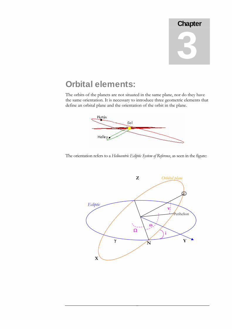
Orbital elements: The orbits of the planets are not situated in the same plane, nor do they have the same orientation. It is necessary to introduce three geometric elements that define an orbital plane and the orientation of the orbit in the plane.

The orientation refers to a Heliocentric Ecliptic System of Reference, as seen in the figure:

X

Z

Y γ

Ecliptic

Orbital plane

N

Perihelion

Ω

v

ω

i

8

and the new elements are:

- inclination of the orbital plane with respect to the ecliptic, i

- ecliptic longitude of the ascending node, Ω

- argument of perihelion or angle between the ascending node (N) and the direction of the perihelion, ω

Instead of the parameter ω, a new parameter is commonly used:

Ω+= ωω~

called longitude of perihelion.

In summary, the parameters, i, ω , Ω, a, e, 0τ define a unique orbit. These

parameters are called orbital elements.

Orbital elements for all of the bodies in the Solar System (and also for satellites in orbit around the Earth) vary over time. The gravitational action of other bodies converts the two-body problem into a problem of N-bodies, which is not integrable, and needs to be solved numerically.

9

ORBITAL ELEMENTS OF THE PLANETS OF THE SOLAR SYSTEM

Planet

a

(a.u.)

e Ω

(º)

ϖ

(º)

i

(º)

L(τ) = M(τ)+ϖ

τ=4/June/2004 TU:00

Mercury 0.3871 0.2056 48.33 77.5 7.00 23.49

Venus 0.7233 0.0068 76.68 131.7 3.39 250.28

Earth 1.0000 0.0167 - 102.9 0.00 252.78

Mars 1.5237 0.0934 49.58 336.1 1.85 122.09

Jupiter 5.2026 0.0485 100.45 14.8 1.30 168.63

Saturn 9.5548 0.0555 113.66 94.3 2.49 104.32

Uranus 19.1817 0.0473 74.00 170.3 0.77 332.22

Neptune 30.0583 0.0086 131.78 67.7 1.77 314.50

Pluto 39.4817 0.2488 110.30 223.8 17.16 245.97

10

Chapter

4

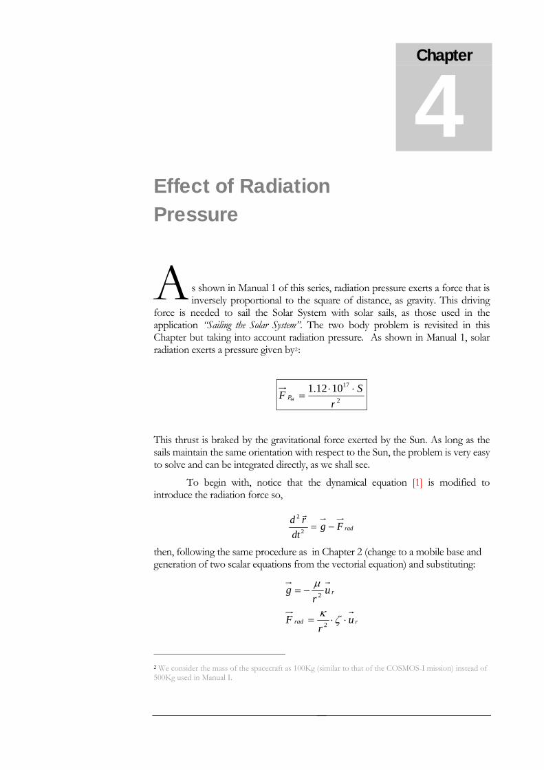
Effect of Radiation Pressure

s shown in Manual 1 of this series, radiation pressure exerts a force that is inversely proportional to the square of distance, as gravity. This driving

force is needed to sail the Solar System with solar sails, as those used in the application “Sailing the Solar System”. The two body problem is revisited in this Chapter but taking into account radiation pressure. As shown in Manual 1, solar radiation exerts a pressure given by2:

A

2

171012.1r

SF P⋅⋅

=Θ

This thrust is braked by the gravitational force exerted by the Sun. As long as the sails maintain the same orientation with respect to the Sun, the problem is very easy to solve and can be integrated directly, as we shall see.

To begin with, notice that the dynamical equation [1] is modified to introduce the radiation force so,

radFgdt

rd−=2

2 r

then, following the same procedure as in Chapter 2 (change to a mobile base and generation of two scalar equations from the vectorial equation) and substituting:

rrad

r

ur

F

ur

g

⋅⋅=

−=

ζκ

μ

2

2

2 We consider the mass of the spacecraft as 100Kg (similar to that of the COSMOS-I mission) instead of 500Kg used in Manual I.

11

with, μ=G(M+m) and ζ=Scosϕ, we obtain:

( )

ctehrrr

rrrrr

==⋅⇒=⋅+⋅

⋅−−=⋅+−=⋅−

•••••

•••

θθθ

ζκμζκμθ

2

222

2

02

So, making the change of variable, u

r 1= :

( ) ( ) 023

2

24

2

=⋅−

+−=⋅−

+⋅−••••

rrhr

rrhrr ζκμζκμ

and,

2

222

22

2

2

2

2

2

2

1

θθθ

θθ

θθθθ

θ

duduh

rh

dudh

dtd

dudh

ddu

dtdh

dtrd

dduh

ddu

udtd

ddu

dudr

dtdr

−=⎟⎠⎞

⎜⎝⎛−=−=⎟

⎠⎞

⎜⎝⎛⋅−=

⋅−=⋅⋅−== &

[3]

we obtain:

⎟⎠⎞

⎜⎝⎛ ⋅−

=+ 22

2

hu

dud ζκμ

θ

To bring in numbers, it is necessary to substitute the constants in the problem for realistic values. In the application “Sailing the Solar System”, we have considered that the spacecraft leaves a space station at L1- i.e. co-orbiting with the Earth around the Sun. Therefore, the angular momentum per unit of mass of the spacecraft will be very similar to that of the Earth:

1219105.4 −⋅= scmh

If the mass of the spacecraft is similar to that of the prototype COSMOS-I (100 kg), then:

gdinas171012.1 ⋅=κ

and μ=1.33⋅1026 g⋅cm3s-2. So,

℘=⋅−⋅=+ −− )(1053.51057.6 223142

2

cmud

ud ζθ

12

where ℘ is a constant for the fixed orientation of the Solar Sails.

Therefore, the radiation pressure will only have a significant effect on the trajectory if the surface of the ship is around 109cm2 or 105m2. The size proposed for the sail in the application (100,000m2 is the surface of a circle of a radius of 178m), is derived from this estimate. The solution to the equation is:

℘+−= )cos(10θθA

r

with θ0 and A constants of integration.

If we set the origin of the angles at the point of greatest proximity of the spacecraft to the Sun, then θ0=0 and, in addition,

℘+= Arperihelio

1

Let us suppose that the distance from the spacecraft to the Sun in the perihelion is approximately equal to the average distance Sun-Earth(1.49⋅1013cm). In this case, the value of the constant A will depend on the projected surface of the sails, ζ, as,

)(1053.51033.8 21914 mA ς−− ⋅−⋅=

where A is given in cm-1.

θcos)/(1/1

⋅℘+℘

=A

r

Thus orbit of a solar sail ship (that keeps the sails always oriented in the same direction in relation to the Sun) is an ellipse, although, for the same value of ε, the eccentricity of the orbit would be much larger than the purely gravitational orbital motion.

Finally, observe that vector rr points to the Sun as, on defining our mobile base of vectors, we chose mM rrr rrr

−= .

13

X

Y

Z

Mrr

mrr

rr

Components of the velocity vector: At any moment, the components of velocity of the spacecraft (assuming ζ as a constant) will be:

θ

Vθ

Vr

V φ

Azimutal Velocity: Vθ

For a ship leaving the orbit of the Earth, Vθ is given in a direct way by the constant, h, the constant angular momentum

rrh

rhrrV

19

2

105.4 ⋅==== θθ

&

if we wish to give r in astronomic units (see Manual I) and obtain Vθ in km/s,

.).(/20.30

aurskmV =θ

14

Radial velocity: Vr

Radial velocity must be calculated from this equation [3],

[4]θsenAhrVr ⋅⋅== &

substituting the constants h and A, we obtain:

[ ] θϕ senmSskmskmVr ⋅⋅⋅⋅−= − cos)(/1048.2/49.37 24

Notice that, depending on the effective surface of the sail, the radial velocity will fluctuate between very small or very large values. Another way of visualising this effect is by substituting sinθ for its value depending on r, in equation [4],

22

2

22 11111cos1 ⎟

⎠⎞

⎜⎝⎛ ℘−−=⎟

⎠⎞

⎜⎝⎛ ℘−−=−=

rA

ArAsen θθ

so that,

22

2

1⎟⎠⎞

⎜⎝⎛ ℘−−

⋅=

rA

AhVr

General considerations on the trajectory and value of the energy constant: The integration constant, A, is fixed by the energy per unit of mass in the orbit, as we have seen in Chapter 1. Therefore, it is usual to give Vr directly as a function of the energy per unit of mass, ε. This energy is the sum of the kinetic and potential energy:

22222 )(21)(

21 h

rVV

rrVV rrpc

℘−+=⎟

⎠⎞

⎜⎝⎛ ⋅

+−++=+= θθςκμεεε

and,

⎥⎦

⎤⎢⎣

⎡⎟⎟⎠

⎞⎜⎜⎝

⎛ ℘−−=

⎥⎥⎦

⎤

⎢⎢⎣

⎡ ℘+−⋅= 2

2

22

2

22

22 h

rrhh

rV

Vr εε θ

Notice that Vr represents the modulus of the radial velocity, i.e., Vr ≥ 0; this sets important constraints on the radical once ε is fixed. It is usual to define a function Φ(r) or Effective Potential, such that,

15

⎟⎠⎞

⎜⎝⎛ ℘

−=Φrr

hr 22

21)(

and substituting the constants,

( ) ( )⎟⎟⎠

⎞⎜⎜⎝

⎛ ⋅−⋅−⋅=Φ

−−

rrgergr ξ1414

239 1002.51057.6

21/1002.2)(

where, for convenience , we have introduced a new constant, ξ, to give us the fraction of the maximum possible surface total surface ξ0=9.0792⋅104m2 (equivalent to the surface of a circle with a radius of 170 m), covered by the sail,

4

2

100792.9cos)(⋅

=ϕξ mS

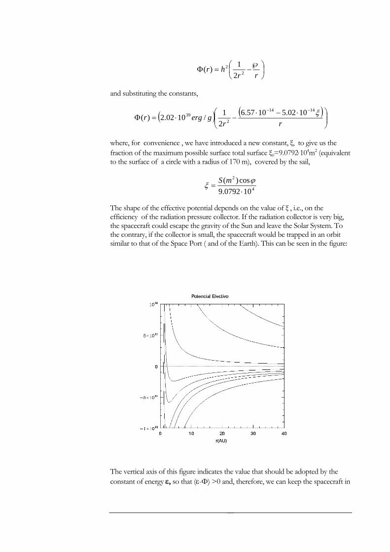
The shape of the effective potential depends on the value of ξ , i.e., on the efficiency of the radiation pressure collector. If the radiation collector is very big, the spacecraft could escape the gravity of the Sun and leave the Solar System. To the contrary, if the collector is small, the spacecraft would be trapped in an orbit similar to that of the Space Port ( and of the Earth). This can be seen in the figure:

The vertical axis of this figure indicates the value that should be adopted by the constant of energy ε, so that (ε-Φ) >0 and, therefore, we can keep the spacecraft in

16

this position. The most negative curve corresponds to ξ=0.1 and the most positive to ξ=10. In the first case, the solar sail ship does not get enough thrust from solar radiation to escape the Space Port and will remain trapped in a nearby orbit. In contrast, if ξ=10, the spacecraft gets an enormous push from radiation and easily leaves the Port and the Solar System.

In practice, the value of ε is very small, , at the Earth orbit and any reasonably sized sail (like the one proposed for the prototype Cosmos I) could not make it. In the application, we have used unrealistically high values for the surface to allow the students to play with the thrust of Solar Radiation. If they fill up a significant fraction of the total available surface (the circle at the begining of the application) they should be able to significantly modify V

gerg /1048.4 12⋅−

r and thus the direction of the total velocity vector. This opens up the “launching windows” for solar sail ships. The objective of the application is to strengthen some basic concepts in Physics.

Notice that the “launching angle” or angle that the ship velocity makes with the vector Sun-Spacecraft is:

θ

φVVr=tan

Thus φ can be varied by modifying Vr that, in turn, can be modified by turning the sails (i.e. changing ϕ) since:

ϕcos)(1048.249.37)/( 24 mSskmVr−⋅−=

The students are to go through this set of operations:

1. adjusting Vr with the graphic interface to launch the ship in the desired direction (get the resultant vector V aligned with the Space Port-Saturn direction)

2. the projected surface needed to get this resultant is calculated internally from:

42

1048.249.37cos)( −⋅

−= rVmS ϕ

and given to the student by the application.

3. Later, students determine the projection angle ϕ using the surface of the sail as designed by them and the projected surface provided by the application.

17

Appendix

1

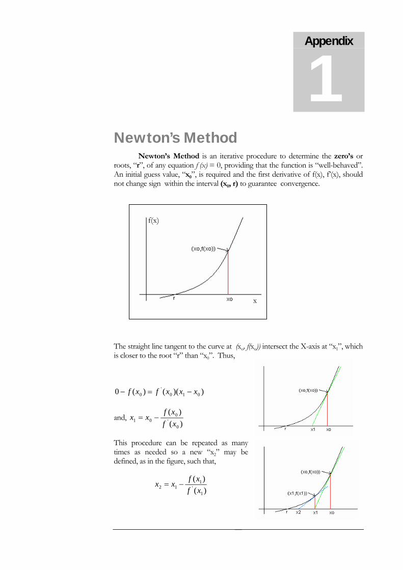
Newton’s Method Newton’s Method is an iterative procedure to determine the zero’s or roots, “r”, of any equation f (x) = 0, providing that the function is “well-behaved”. An initial guess value, “x0”, is required and the first derivative of f(x), f’(x), should not change sign within the interval (x0, r) to guarantee convergence.

f(x)

x

The straight line tangent to the curve at (xo, f(xo)) intersect the X-axis at “x1”, which is closer to the root “r” than “x0”. Thus,

))(()(0 010'

0 xxxfxf −=−

and, )()(

0'

001 xf

xfxx −=

This procedure can be repeated as many times as needed so a new “x2” may be defined, as in the figure, such that,

)()(

1'

112 xf

xfxx −=

18

and, in general, the recurrence formula: )()(

'1n

nnn xf

xfxx −=+ (*)

Application to the resolution of Kepler’s equation: To find the solution to Kepler’s equation is equivalent to find the zeros of

the function f(E) such that:

senEeEMEf ⋅+−=)(

and making use of the Newton’s method(*):

)cos(1)(')()(

nn

nnn

nn

EEfEseneEMEf

Ex

+−=⋅+−=

=

then,

n

nnnn

n

nnn

EsenEeEM

EE

EfEf

EE

cos1

;)()(

1

'1

+−⋅+−

−=

−=

+

+

and,

n

nnnn E

senEeEMEE

cos11 −⋅+−

+=+

taking in the first iteration E0 = M3

3 Note: Angular values must be expressed in radians.

19