Universal Reinforcement Learning Algorithms: … Reinforcement Learning Algorithms: Survey and ... class of models hypothesesenvironments M . ... Universal Reinforcement Learning Algorithms:

Universal Reinforcement Learning Algorithms: Survey and Experiments

John Aslanides†, Jan Leike‡∗, Marcus Hutter††Australian National University

‡Future of Humanity Institute, University of Oxford{john.aslanides, marcus.hutter}@anu.edu.au, [email protected]

AbstractMany state-of-the-art reinforcement learning (RL)algorithms typically assume that the environmentis an ergodic Markov Decision Process (MDP). Incontrast, the field of universal reinforcement learn-ing (URL) is concerned with algorithms that makeas few assumptions as possible about the environ-ment. The universal Bayesian agent AIXI and afamily of related URL algorithms have been de-veloped in this setting. While numerous theoret-ical optimality results have been proven for theseagents, there has been no empirical investigationof their behavior to date. We present a short andaccessible survey of these URL algorithms undera unified notation and framework, along with re-sults of some experiments that qualitatively illus-trate some properties of the resulting policies, andtheir relative performance on partially-observablegridworld environments. We also present an open-source reference implementation of the algorithmswhich we hope will facilitate further understandingof, and experimentation with, these ideas.

1 IntroductionThe standard approach to reinforcement learning typically as-sumes that the environment is a fully-observable Markov De-cision Process (MDP) [Sutton and Barto, 1998]. Many state-of-the-art applications of reinforcement learning to largestate-action spaces are achieved by parametrizing the policywith a large neural network, either directly (e.g. with deepdeterministic policy gradients [Silver et al., 2014]) or indi-rectly (e.g. deep Q-networks [Mnih et al., 2013]). These ap-proaches have yielded superhuman performance on numer-ous domains including most notably the Atari 2600 videogames [Mnih et al., 2015] and the board game Go [Silver etal., 2016]. This performance is due in large part to the scal-ability of deep neural networks; given sufficient experienceand number of layers, coupled with careful optimization, adeep network can learn useful abstract features from high-dimensional input. These algorithms are however restrictedin the class of environments that they can plausibly solve,∗Now at DeepMind.

due to the finite capacity of the network architecture and themodelling assumptions that are typically made, e.g. that theoptimal policy can be well-approximated by a function of afully-observable state vector.

In the setting of universal reinforcement learning, we liftthe Markov, ergodic, and full-observability assumptions, andattempt to derive algorithms to solve this general class of en-vironments. URL aims to answer the theoretical question:“making as few assumptions as possible about the environ-ment, what constitutes optimal behavior?”. To this end sev-eral Bayesian, history-based algorithms have been proposedin recent years, central of which is the agent AIXI [Hutter,2005]. Numerous important open conceptual questions re-main [Hutter, 2009], including the need for a relevant, ob-jective, and general optimality criterion [Leike and Hutter,2015a]. As the field of artifical intelligence research movesinexorably towards AGI, these questions grow in import andrelevance.

The contribution of this paper is three-fold: we present asurvey of these URL algorithms, and unify their presentationunder a consistent vocabulary. We illuminate these agentswith an empirical investigation into their behavior and prop-erties. Apart from the MC-AIXI-CTW implementation [Ve-ness et al., 2011] this is the only non-trivial set of experimentsrelating to AIXI, and is the only set of experiments relatingto its variants; hitherto only their asymptotic properties havebeen studied theoretically. Our third contribution is to presenta portable and extensible open-source software framework1

for experimenting with, and demonstrating, URL algorithms.We also discuss several tricks and approximations that are re-quired to get URL implementations working in practice. Ourdesire is that this framework will be of use, both for educationand research, to the RL and AI safety communities.2

2 Literature SurveyThis survey covers history-based Bayesian algorithms; wechoose history-based algorithms, as these are maximally gen-eral, and we restrict ourselves to Bayesian algorithms, as

1The framework is named AIXIJS; the source code can be foundat http://github.com/aslanides/aixijs.

2A more comprehensive introduction and discussion includingmore experimental results can be found in the associated thesis athttps://arxiv.org/abs/1705.07615.

Proceedings of the Twenty-Sixth International Joint Conference on Artificial Intelligence (IJCAI-17)

1403

they are generally both principled and theoretically tractable.The universal Bayesian agent AIXI [Hutter, 2005] is a modelof a maximally intelligent agent, and plays a central rolein the sub-field of universal reinforcement learning (URL).Recently, AIXI has been shown to be flawed in importantways; in general it doesn’t explore enough to be asymptot-ically optimal [Orseau, 2010], and it can perform poorly,even asymptotically, if given a bad prior [Leike and Hutter,2015a]. Several variants of AIXI have been proposed to at-tempt to address these shortfalls: among them are entropy-seeking [Orseau, 2011], information-seeking [Orseau et al.,2013], Bayes with bursts of exploration [Lattimore, 2013],MDL agents [Leike, 2016], Thompson sampling [Leike et al.,2016], and optimism [Sunehag and Hutter, 2015].

It is worth emphasizing that these algorithms are modelsof rational behavior in general environments, and are not in-tended to be efficient or practical reinforcement learning al-gorithms. In this section, we provide a survey of the abovealgorithms, and of relevant theoretical results in the universalreinforcement learning literature.

2.1 NotationAs we are discussing POMDPs, we distinguish between (hid-den) states and percepts, and we take into account histories,i.e. sequences of actions and percepts. States, actions, andpercepts use Latin letters, while environments and policiesuse Greek letters. We use R as the reals, and B = {0, 1}.For sequences over some alphabet X , X k is the set of allsequences≈strings of length k over X . We typically use theshorthand x1:k := x1x2 . . . xk and x<k := x1:k−1. Concate-nation of two strings x and y is given by xy. We refer toenvironments and environment models using the symbol ν,and distinguish the true environment with µ. The symbol εis used to represent the empty string, while ε is used to rep-resent a small positive number. The symbols → and aredeterministic and stochastic mappings, respectively.

2.2 The General Reinforcement Learning ProblemWe begin by formulating the agent-environment interac-tion. The environment is modelled as a partially observableMarkov Decision Process (POMDP). That is, we can assumewithout loss of generality that there is some hidden state swith respect to which the environment’s dynamics are Marko-vian. Let the state space S be a compact subset of a finite-dimensional vector space RN . For simplicity, assume thatthe action spaceA is finite. By analogy with a hidden Markovmodel, we associate with the environment stochastic dynam-ics D : S × A S . Because the environment is in generalpartially observable, we define a percept space E . Perceptsare distributed according to a state-conditional percept distri-bution ν; as we are largely concerned with the agent’s per-spective, we will usually refer to ν as the environment itself.

The agent selects actions according to a policy π ( · |æ<t),a conditional distribution over A. The agent-environment in-teraction takes the form of a two-player, turn-based game;the agent samples an action at ∈ A from its policyπ ( · |æ<t), and the environment samples a percept et ∈ Efrom ν ( · |æ<tat). Together, they interact to produce a his-tory: a sequence of action-percept pairs h<t ≡ æ<t :=

a1e1 . . . at−1et−1. The agent and environment together in-duce a telescoping distribution over histories, analogous tothe state-visit distribution in RL:

νπ (æ1:t) :=t∏

k=1

π (ak|æ<k) ν (ek|æ<kak) . (1)

In RL, percepts consist of (observation, reward) tuples sothat et = (ot, rt). We assume that the reward signal is real-valued, rt ∈ R, and make no assumptions about the structureof the ot ∈ O. In general, agents will have some utility func-tion u that typically encodes some preferences about states ofthe world. In the partially observable setting, the agent willhave to make inferences from its percepts to world-states. Forthis reason, the utility function is a function over finite histo-ries of the form u (æ1:t); for agents with an extrinsic rewardsignal, u (æ1:t) = rt. The agent’s objective is to maximizeexpected future discounted utility. We assume a general classof convergent discount functions, γtk : N × N → [0, 1] withthe property Γtγ :=

∑∞k=t γ

tk < ∞. For this purpose, we

introduce the value function, which in this setting pertains tohistories rather than states:

V πuνγ (æ<t) := Eπν

[ ∞∑k=t

γtku (æ1:k)

∣∣∣∣∣æ<t

]. (2)

In words, V πuνγ is the expected discounted future sum of re-ward obtained by an agent following policy π in environmentν under discount function γ and utility function u. For con-ciseness we will often drop the γ and/or µ subscripts from Vwhen the discount/utility functions are irrelevant or obviousfrom context; by default we assume geometric discountingand extrinsic rewards. The value of an optimal policy is givenby the expectimax expression

V ?uνγ (æ<t) = maxπ

V πuνγ

= limm→∞

maxat∈A

∑et∈E· · · max

at+m∈A

∑et+m∈E

(t+m∑k=t

γtku (æ1:k)k∏j=t

ν (ej |æ<jaj)

)(3)

which follows from Eqs. (1) and (2) by jointly maximiz-ing over all future actions and distributing max over

∑. The

optimal policy is then simply given by π?ν = arg maxπ Vπν ;

note that in general the optimal policy may not exist if u is un-bounded from above. We now introduce the only non-trivialand non-subjective optimality criterion yet known for gen-eral environments [Leike and Hutter, 2015a]: weak asymp-totic optimality.Definition 1 (Weak asymptotic optimality; Lattimore & Hut-ter, 2011). Let the environment classM be a set of environ-ments. A policy π is weakly asymptotically optimal inM if∀µ ∈M, V πµ → V ∗µ in mean, i.e.

µπ

(limn→∞

1

n

n∑t=1

{V ∗µ (æ<t)− V πµ (æ<t)

}= 0

)= 1,


1404

where µπ is the history distribution defined in Equation (1).

AIXI is not in general asymptotically optimal, but bothBayesExp and Thompson sampling (introduced below) are.Finally, we introduce the the notion of effective horizon,which these algorithms rely on for their optimality.

Definition 2 (ε-Effective horizon; Lattimore & Hutter, 2014).Given a discount function γ, the ε-effective horizon is givenby

Htγ (ε) := min

{H :

Γt+Hγ

Γtγ≤ ε

}. (4)

In words,H is the horizon that one can truncate one’s plan-ning to while still accounting for a fraction equal to (1− ε)of the realizable return under stationary i.i.d. rewards.

2.3 AlgorithmsWe consider the class of Bayesian URL agents. The agentsmaintain a predictive distribution over percepts, that we calla mixture model ξ. The agent mixes≈marginalizes over aclass of models≈hypotheses≈environmentsM. We considercountable nonparametric model classesM so that

ξ (e) =∑ν∈M

ν(e)︷︸︸︷p (e|ν) p (ν)︸︷︷︸

wν

, (5)

where we have suppressed the conditioning on historyæ<tat for clarity. We have identified the agent’s credence inhypothesis ν with weights wν , with wν > 0 and

∑ν wν ≤ 1,

and we write the probability that ν assigns to percept eas ν (e). We update with Bayes rule, which amounts top (ν|e) = p(e|ν)

p(e) p (ν), which induces the sequential weight

updating scheme wν ← ν(e)ξ(e)wν ; see Algorithm 1. We will

sometimes use the notation wν|æ<t to represent the posteriormass on ν after updating on history æ<t ∈ (A× E)

∗, andw (· | ·) when referring explicitly to a posterior distribution.

Definition 3 (AIξ; Hutter, 2005). AIξ is the policy that isoptimal w.r.t. the Bayes mixture ξ:

π?ξ := arg maxπ

V πξ

= limm→∞

arg maxat∈A

∑et∈E· · · max

am∈A

∑em∈E

(m∑k=t

γkrk

k∏j=t

∑ν∈M

wνν (ej |æ<jaj)

. (6)

Computational tractability aside, a central issue inBayesian induction lies in the choice of prior. If computa-tional considerations aren’t an issue, we can chooseM to beas broad as possible: the class of all lower semi-computableconditional contextual semimeasuresMLSC

CCS [Leike and Hut-ter, 2015b], and using the prior wν = 2−K(ν), where Kis the Kolmogorov complexity. This is equivalent to usingSolomonoff’s universal prior [Solomonoff, 1978] over stringsM (x) :=

∑q : U(q)=x∗ 2−|q|, and yields the AIXI model.

AIξ is known to not be asymptotically optimal [Orseau,2010], and it can be made to perform badly by bad priors[Leike and Hutter, 2015a].

Algorithm 1 Bayesian URL agent [Hutter, 2005]Inputs: Model classM = {ν1, . . . , νK}; prior w : M →

(0, 1); history æ<t.

1: function ACT(π)2: Sample and perform action at ∼ π(·|æ<t)3: Receive et ∼ ν( · |æ<tat)4: for ν ∈M do5: wν ← ν(et|æ<tat)

ξ(et|æ<tat)wν6: end for7: t← t+ 18: end function

Knowledge-seeking agents (KSA). Exploration is one ofthe central problems in reinforcement learning [Thrun, 1992],and a principled and comprehensive solution does not yetexist. With few exceptions, the state-of-the-art has not yetmoved past ε-greedy exploration [Bellemare et al., 2016;Houthooft et al., 2016; Pathak et al., 2017; Martin et al.,2017]. Intrinsically motivating an agent to explore in envi-ronments with sparse reward structure via knowledge-seekingis a principled and general approach. This removes the de-pendence on extrinsic reward signals or utility functions, andcollapses the exploration-exploitation trade-off to simply ex-ploration. There are several generic ways in which to for-mulate a knowledge-seeking utility function for model-basedBayesian agents. We present three, due to Orseau et al.:Definition 4 (Kullback-Leibler KSA; Orseau, 2014). TheKL-KSA is the Bayesian agent whose utility function is givenby the information gain

uKL (æ1:t) = IG (et) (7):= Ent (w (·|æ<t))− Ent (w (·|æ1:t)) . (8)

Informally, the KL-KSA gets rewarded for reducing the en-tropy (uncertainty) in its model. Now, note that the entropy inthe Bayesian mixture ξ can be decomposed into contributionsfrom uncertainty in the agent’s beliefswν and noise in the en-vironment ν. That is, given a mixture ξ and for some percepte such that 0 < ξ (e) < 1, and suppressing the history æ<tat,

ξ (e) =∑ν∈M

uncertainty︷︸︸︷wν ν (e)︸︷︷︸

noise

.

That is, if 0 < wν < 1, we say the agent is uncertainabout whether hypothesis ν is true (assuming there is ex-actly one µ ∈ M that is the truth). On the other hand, if0 < ν (e) < 1 we say that the environment ν is noisy orstochastic. If we restrict ourselves to deterministic environ-ments such that ν (e) ∈ {0, 1} ∀ν ∀e, then ξ (·) ∈ (0, 1) im-plies that wν ∈ (0, 1) for at least one ν ∈ M. This motivatesus to define two agents that seek out percepts to which themixture ξ assigns low probability; in deterministic environ-ments, these will behave like knowledge-seekers.


1405

Definition 5 (Square & Shannon KSA; Orseau, 2011). TheSquare and Shannon KSA are the Bayesian agents with utilityu (æ1;t) given by −ξ (æ1:t) and − log ξ (æ1:t) respectively.

Square, Shannon, and KL-KSA are so-named becauseof the form of the expression when one computes the ξ-expected utility: this is clear for Square and Shannon, andfor KL it turns out that the expected information gain isequal to the posterior weighted KL-divergence Eξ [IG] =∑ν∈M wν|eKL (ν‖ξ) [Lattimore, 2013]. Note that as far

as implementation is concerned, these knowledge-seekingagents differ from AIξ only in their utility functions.

The following two algorithms (BayesExp and Thompsonsampling) are RL agents that add exploration heuristics soas to obtain weak asymptotic optimality, at the cost of in-troducing an exploration schedule {ε1, ε2, . . . } which can beannealed, i.e. εt ≤ εt−1 and εt → 0 as t→∞.

BayesExp. BayesExp (Algorithm 2) augments the Bayesagent AIξ with bursts of exploration, using the information-seeking policy of KL-KSA. If the expected informationgain exceeds a threshold εt, the agent will embark on aninformation-seeking policy π?,IGξ = arg maxπ V

π,IGξ for one

effective horizon, where IG is defined in Equation (7).

Algorithm 2 BayesExp [Lattimore, 2013]Inputs: Model classM; priorw : M→ (0, 1); exploration

schedule {ε1, ε2, . . . }.

1: loop2: if V ∗,IGξ (æ<t) > εt then3: for i = 1→ Ht

γ (εt) do

4: ACT(π?,IGξ

)5: end for6: else7: ACT

(π?ξ

)8: end if9: end loop

Thompson sampling. Thompson sampling (TS) is a verycommon Bayesian sampling technique, named for [Thomp-son, 1933]. In the context of general reinforcement learn-ing, it can be used as another attempt at solving the explo-ration problems of AIξ. From Algorithm 3, we see that TSfollows the ρ-optimal policy for an effective horizon beforere-sampling from the posterior ρ ∼ w (·|æ<t). This commitsthe agent to a single hypothesis for a significant amount oftime, as it samples and tests each hypothesis one at a time.

MDL. The minimum description length (MDL) principleis an inductive bias that implements Occam’s razor, originallyattributed to [Rissanen, 1978]. The MDL agent greedily picksthe simplest probable unfalsified environment σ in its modelclass and behaves optimally with respect to that environmentuntil it is falsified. If µ ∈ M, Algorithm 4 converges withσ → µ. Note that line 2 of Algorithm 4 amounts to maximumlikelihood regularized by the Kolmogorov complexity K.

Algorithm 3 Thompson Sampling [Leike et al., 2016]Inputs: Model classM; priorw : M→ (0, 1); exploration

schedule {ε1, ε2, . . . }.

1: loop2: Sample ρ ∼ w (·|æ<t)3: d← Ht (εt)4: for i = 1→ Ht (εt) do5: ACT

(π?ρ)

6: end for7: end loop

Algorithm 4 MDL Agent [Lattimore and Hutter, 2011].Inputs: Model classM; prior w : M→ (0, 1), regularizer

constant λ ∈ R+.

1: loop2: σ ← arg minν∈M

[K(ν)− λ

∑tk=1 log ν(ek|æ<kak)

]3: ACT (π?σ)4: end loop

3 ImplementationIn this section, we describe the environments that we use inour experiments, introduce two Bayesian environment mod-els, and discuss some necessary approximations.

3.1 GridworldWe run our experiments on a class of partially-observablegridworlds. The gridworld is an N ×N grid of tiles; tiles canbe either empty, walls, or stochastic reward dispenser tiles.The action space is given by A = {←,→, ↑, ↓, ∅}, whichmove the agent in the four cardinal directions or stand still.The observation space is O = B4, the set of bit-strings oflength four; each bit is 1 if the adjacent tile in the correspond-ing direction is a wall, and is 0 otherwise. The reward spaceis small, and integer-valued: the agent receives r = −1 forwalking over empty tiles, r = −10 for bumping into a wall,and r = 100 with some fixed probability θ if it is on a rewarddispenser tile. There is no observation to distinguish emptytiles from dispensers. In this environment, the optimal pol-icy (assuming unbounded episode length) is to move to thedispenser with highest payout probability θ and remain there,subsequently collecting 100θ reward per cycle in expectation(the environment is non-episodic). In all cases, the agent’sstarting position is at the top left corner at tile (0, 0).

This environment has small action and percept spaces andrelatively straightforward dynamics. The challenge lies incoping with perceptual aliasing due to partial observability,dealing with stochasticity in the rewards, and balancing ex-ploration and exploitation. In particular, for a gridworld withn dispensers with θ1 > θ2 > θn, the gridworld presents anon-trivial exploration/exploitation dilemma; see Figure 1.

3.2 ModelsGenerically, we would like to construct a Bayes mixtureover a model class M that is as rich as possible. Since


1406

we are using a nonparametric model, we are not concernedwith choosing our model class so as to arrange for conjugateprior/likelihood pairs. One might consider constructing Mby enumerating all N ×N gridworlds of the class describedabove, but this is infeasible as the size of such an enumera-tion explodes combinatorially: using just two tile types wewould run out of memory even on a modest 6 × 6 gridworldsince |M| = 236 ≈ 7 × 1010. Instead, we choose a dis-crete parametrization D that enumerates an interesting subsetof these gridworlds. One can think of D as describing a setof parameters about which the agent is uncertain; all otherparameters are held constant, and the agent is fully informedof their value. We use this to create the first of our modelclasses,Mloc. The second,MDirichlet, uses a factorized distri-bution rather than an explicit mixture to avoid this issue.

Mloc. This is a Bayesian mixture parametrized by goallocation; the agent knows the layout of the gridworld andknows its dynamics, but is uncertain about the location of thedispensers, and must explore the world to figure out wherethey are. We construct the model class by enumerating eachof these gridworlds. For square gridworlds of side length N ,|Mloc| = N2. From Algorithm 1 the time complexity of ourBayesian updates is O (|M|) = O

(N2).

MDirichlet. The Bayes mixture Mloc is a natural class ofgridworlds to consider, but it is quite constrained in that itholds the maze layout and dispenser probabilities fixed. Weseek a model that allows the agent to be uncertain about thesefeatures. To do this we move away from the mixture formal-ism so as to construct a bespoke gridworld model.

Let sij ∈ {EMPTY,WALL,DISPENSER, . . . } be the stateof tile (i, j) in the gridworld. The joint distribution over allgridworlds s11, . . . , sNN factorizes across tiles, and the state-conditional percept distributions are Dirichlet over the fourtile types. We effectively use a Haldane prior – Beta (0, 0)– with respect to WALLs and a Laplace prior – Beta (1, 1) –with respect to DISPENSERs. This model class allows us tomake the agent uncertain about the maze layout, including thenumber, location, and payout probabilities of DISPENSERs.In contrast toMloc, model updates areO(1) time complexity,makingMDirichlet a far more efficient choice for large N .

This model class incorporates more domain knowledge,and allows the agent to flexibly and cheaply represent a muchlarger class of gridworlds than using the naive enumerationMloc. Importantly, MDirichlet is still a Bayesian model – wesimply lose the capacity to represent it explicitly as a mixtureof the form of Equation (5).

3.3 Agent ApproximationsPlanning. In contrast to model-free agents, in which thepolicy is explicitly represented by e.g. a neural network,our model-based agents need to calculate their policy fromscratch at each time step by computing the value functionin Equation (6). We approximate this infinite forsight witha finite horizon m > 0, and we approximate the expecta-tion using Monte Carlo techniques. We implement the ρUCTalgorithm [Silver and Veness, 2010; Veness et al., 2011],a history-based version of the UCT algorithm [Kocsis andSzepesvari, 2006]. UCT is itself a variant of Monte CarloTree Search (MCTS), a commonly used planning algorithm

originally developed for computer Go. The key idea is to tryto avoid wasting time considering unpromising sequences ofactions; for this reason the action selection procedure withinthe search tree is motivated by the upper confidence bound(UCB) algorithm [Auer et al., 2002]:

aUCT = arg maxa∈A

(1

m (β − α)V (æ<ta) + C

√log T (æ<t)

T (æ<ta)

),

(9)where T (æ<t) is the number of times the sampler has

reached history æ<t, V (æ<ta) is the current estimator ofV (æ<ta), m is the planning horizon, C is a free parame-ter (usually set to

√2), and α and β are the minimum and

maximum rewards emitted by the environment. In this way,the MCTS planner approximates the expectimax expressionin Equation (3), and effectively yields a stochastic policy ap-proximating π defined in Equation (6) [Veness et al., 2011].

In practice, MCTS is very computationally expensive;when planning by forward simulation with a Bayes mix-ture ξ over M, the worst-case time-complexity of ρUCT isO (κm |M| |A|), where κ is the Monte Carlo sample bud-get. It is important to note that ρUCT treats the environmentmodel ξ as a black box: it is agnostic to the environment’sstructure, and so makes no assumptions or optimizations. Forthis reason, planning in POMDPs with ρUCT is quite waste-ful: due to perceptual aliasing, the algorithm considers manyplans that are cyclic in the (hidden) state space of the POMDP.This is unavoidable, and means that in practice ρUCT can bevery inefficient even in small environments.

Effective horizon. Computing the effective horizon ex-actly for general discount functions is not possible in gen-eral, although approximate effective horizons have been de-rived for some common choices of γ [Lattimore, 2013]. Formost realistic choices of γ and ε, the effective horizonHγ (ε)is significantly greater than the planning horizon m we canfeasibly use due to the prohobitive computational require-ments of MCTS [Lamont et al., 2017]. For this reason weuse the MCTS planning horizon m as a surrogate for Ht

γ . Inpractice, all but small values of m are feasible, resulting inshort-sighted agents with (depending on the environment andmodel) suboptimal and highly stochastic policies.

Utility bounds. Recall from Equation (9) that theρUCT value estimator V (æ1:t) is normalized by a factor ofm (β − α). For reward-based reinforcement learners, α andβ are part of the metadata provided to the agent by the en-vironment at the beginning of the agent-environment inter-action. For utility-based agents such as KSA, however, re-wards are generated intrinsically, and so the agent must cal-culate for itself what range of utilities it expects to see, soas to correctly normalize its value function for the purposesof planning. For Square and KL-KSA, it is possible to getloose utility bounds [α, β] by making some reasonable as-sumptions. Since uSquare (e) = −ξ (e), we have the bound−1 ≤ uSquare ≤ 0. One can argue that for the vast majorityof environments this bound will be tight above, since therewill exist percepts ef that the agent’s model has effectivelyfalsified such that ξ (ef )→ 0 as t→∞.

In the case of the KL-KSA, recall that uKL (e) =


1407

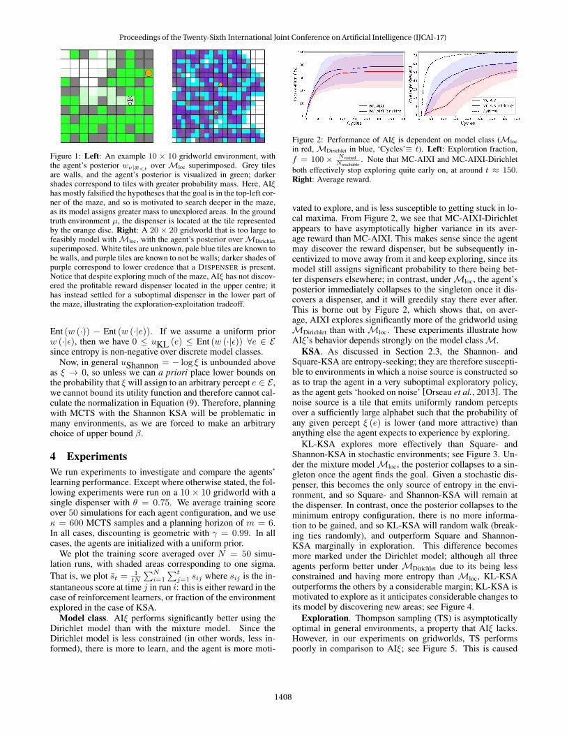
Figure 1: Left: An example 10 × 10 gridworld environment, withthe agent’s posterior wν|æ<t over Mloc superimposed. Grey tilesare walls, and the agent’s posterior is visualized in green; darkershades correspond to tiles with greater probability mass. Here, AIξhas mostly falsified the hypotheses that the goal is in the top-left cor-ner of the maze, and so is motivated to search deeper in the maze,as its model assigns greater mass to unexplored areas. In the groundtruth environment µ, the dispenser is located at the tile representedby the orange disc. Right: A 20 × 20 gridworld that is too large tofeasibly model withMloc, with the agent’s posterior overMDirichletsuperimposed. White tiles are unknown, pale blue tiles are known tobe walls, and purple tiles are known to not be walls; darker shades ofpurple correspond to lower credence that a DISPENSER is present.Notice that despite exploring much of the maze, AIξ has not discov-ered the profitable reward dispenser located in the upper centre; ithas instead settled for a suboptimal dispenser in the lower part ofthe maze, illustrating the exploration-exploitation tradeoff.

Ent (w (·)) − Ent (w (·|e)). If we assume a uniform priorw (·|ε), then we have 0 ≤ uKL (e) ≤ Ent (w (·|ε)) ∀e ∈ Esince entropy is non-negative over discrete model classes.

Now, in general uShannon = − log ξ is unbounded aboveas ξ → 0, so unless we can a priori place lower bounds onthe probability that ξ will assign to an arbitrary percept e ∈ E ,we cannot bound its utility function and therefore cannot cal-culate the normalization in Equation (9). Therefore, planningwith MCTS with the Shannon KSA will be problematic inmany environments, as we are forced to make an arbitrarychoice of upper bound β.

4 ExperimentsWe run experiments to investigate and compare the agents’learning performance. Except where otherwise stated, the fol-lowing experiments were run on a 10 × 10 gridworld with asingle dispenser with θ = 0.75. We average training scoreover 50 simulations for each agent configuration, and we useκ = 600 MCTS samples and a planning horizon of m = 6.In all cases, discounting is geometric with γ = 0.99. In allcases, the agents are initialized with a uniform prior.

We plot the training score averaged over N = 50 simu-lation runs, with shaded areas corresponding to one sigma.That is, we plot st = 1

tN

∑Ni=1

∑tj=1 sij where sij is the in-

stantaneous score at time j in run i: this is either reward in thecase of reinforcement learners, or fraction of the environmentexplored in the case of KSA.

Model class. AIξ performs significantly better using theDirichlet model than with the mixture model. Since theDirichlet model is less constrained (in other words, less in-formed), there is more to learn, and the agent is more moti-

Figure 2: Performance of AIξ is dependent on model class (Mlocin red,MDirichlet in blue, ‘Cycles’≡ t). Left: Exploration fraction,f = 100 × Nvisited

Nreachable. Note that MC-AIXI and MC-AIXI-Dirichlet

both effectively stop exploring quite early on, at around t ≈ 150.Right: Average reward.

vated to explore, and is less susceptible to getting stuck in lo-cal maxima. From Figure 2, we see that MC-AIXI-Dirichletappears to have asymptotically higher variance in its aver-age reward than MC-AIXI. This makes sense since the agentmay discover the reward dispenser, but be subsequently in-centivized to move away from it and keep exploring, since itsmodel still assigns significant probability to there being bet-ter dispensers elsewhere; in contrast, underMloc, the agent’sposterior immediately collapses to the singleton once it dis-covers a dispenser, and it will greedily stay there ever after.This is borne out by Figure 2, which shows that, on aver-age, AIXI explores significantly more of the gridworld usingMDirichlet than withMloc. These experiments illustrate howAIξ’s behavior depends strongly on the model classM.

KSA. As discussed in Section 2.3, the Shannon- andSquare-KSA are entropy-seeking; they are therefore suscepti-ble to environments in which a noise source is constructed soas to trap the agent in a very suboptimal exploratory policy,as the agent gets ‘hooked on noise’ [Orseau et al., 2013]. Thenoise source is a tile that emits uniformly random perceptsover a sufficiently large alphabet such that the probability ofany given percept ξ (e) is lower (and more attractive) thananything else the agent expects to experience by exploring.

KL-KSA explores more effectively than Square- andShannon-KSA in stochastic environments; see Figure 3. Un-der the mixture modelMloc, the posterior collapses to a sin-gleton once the agent finds the goal. Given a stochastic dis-penser, this becomes the only source of entropy in the envi-ronment, and so Square- and Shannon-KSA will remain atthe dispenser. In contrast, once the posterior collapses to theminimum entropy configuration, there is no more informa-tion to be gained, and so KL-KSA will random walk (break-ing ties randomly), and outperform Square and Shannon-KSA marginally in exploration. This difference becomesmore marked under the Dirichlet model; although all threeagents perform better under MDirichlet due to its being lessconstrained and having more entropy than Mloc, KL-KSAoutperforms the others by a considerable margin; KL-KSA ismotivated to explore as it anticipates considerable changes toits model by discovering new areas; see Figure 4.

Exploration. Thompson sampling (TS) is asymptoticallyoptimal in general environments, a property that AIξ lacks.However, in our experiments on gridworlds, TS performspoorly in comparison to AIξ; see Figure 5. This is caused


1408

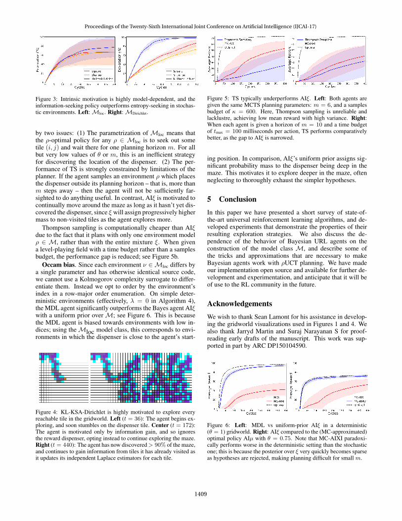
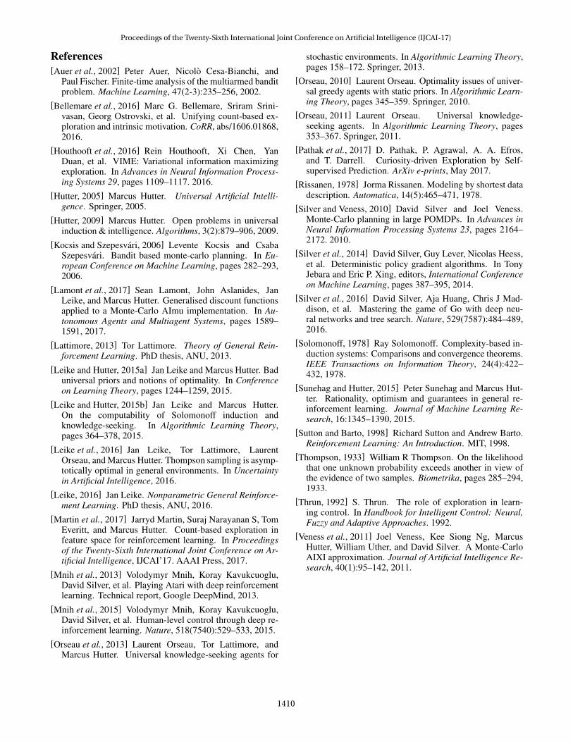
Figure 3: Intrinsic motivation is highly model-dependent, and theinformation-seeking policy outperforms entropy-seeking in stochas-tic environments. Left:Mloc. Right:MDirichlet.

by two issues: (1) The parametrization of Mloc means thatthe ρ-optimal policy for any ρ ∈ Mloc is to seek out sometile (i, j) and wait there for one planning horizon m. For allbut very low values of θ or m, this is an inefficient strategyfor discovering the location of the dispenser. (2) The per-formance of TS is strongly constrained by limitations of theplanner. If the agent samples an environment ρ which placesthe dispenser outside its planning horizon – that is, more thanm steps away – then the agent will not be sufficiently far-sighted to do anything useful. In contrast, AIξ is motivated tocontinually move around the maze as long as it hasn’t yet dis-covered the dispenser, since ξ will assign progressively highermass to non-visited tiles as the agent explores more.

Thompson sampling is computationally cheaper than AIξdue to the fact that it plans with only one environment modelρ ∈ M, rather than with the entire mixture ξ. When givena level-playing field with a time budget rather than a samplesbudget, the performance gap is reduced; see Figure 5b.

Occam bias. Since each environment ν ∈ Mloc differs bya single parameter and has otherwise identical source code,we cannot use a Kolmogorov complexity surrogate to differ-entiate them. Instead we opt to order by the environment’sindex in a row-major order enumeration. On simple deter-ministic environments (effectively, λ = 0 in Algorithm 4),the MDL agent significantly outperforms the Bayes agent AIξwith a uniform prior overM; see Figure 6. This is becausethe MDL agent is biased towards environments with low in-dices; using theMloc model class, this corresponds to envi-ronments in which the dispenser is close to the agent’s start-

Figure 4: KL-KSA-Dirichlet is highly motivated to explore everyreachable tile in the gridworld. Left (t = 36): The agent begins ex-ploring, and soon stumbles on the dispenser tile. Center (t = 172):The agent is motivated only by information gain, and so ignoresthe reward dispenser, opting instead to continue exploring the maze.Right (t = 440): The agent has now discovered> 90% of the maze,and continues to gain information from tiles it has already visited asit updates its independent Laplace estimators for each tile.

Figure 5: TS typically underperforms AIξ. Left: Both agents aregiven the same MCTS planning parameters: m = 6, and a samplesbudget of κ = 600. Here, Thompson sampling is unreliable andlacklustre, achieving low mean reward with high variance. Right:When each agent is given a horizon of m = 10 and a time budgetof tmax = 100 milliseconds per action, TS performs comparativelybetter, as the gap to AIξ is narrowed.

ing position. In comparison, AIξ’s uniform prior assigns sig-nificant probability mass to the dispenser being deep in themaze. This motivates it to explore deeper in the maze, oftenneglecting to thoroughly exhaust the simpler hypotheses.

5 ConclusionIn this paper we have presented a short survey of state-of-the-art universal reinforcement learning algorithms, and de-veloped experiments that demonstrate the properties of theirresulting exploration strategies. We also discuss the de-pendence of the behavior of Bayesian URL agents on theconstruction of the model class M, and describe some ofthe tricks and approximations that are necessary to makeBayesian agents work with ρUCT planning. We have madeour implementation open source and available for further de-velopment and experimentation, and anticipate that it will beof use to the RL community in the future.

AcknowledgementsWe wish to thank Sean Lamont for his assistance in develop-ing the gridworld visualizations used in Figures 1 and 4. Wealso thank Jarryd Martin and Suraj Narayanan S for proof-reading early drafts of the manuscript. This work was sup-ported in part by ARC DP150104590.

Figure 6: Left: MDL vs uniform-prior AIξ in a deterministic(θ = 1) gridworld. Right: AIξ compared to the (MC-approximated)optimal policy AIµ with θ = 0.75. Note that MC-AIXI paradoxi-cally performs worse in the deterministic setting than the stochasticone; this is because the posterior over ξ very quickly becomes sparseas hypotheses are rejected, making planning difficult for small m.


1409

References[Auer et al., 2002] Peter Auer, Nicolo Cesa-Bianchi, and

Paul Fischer. Finite-time analysis of the multiarmed banditproblem. Machine Learning, 47(2-3):235–256, 2002.

[Bellemare et al., 2016] Marc G. Bellemare, Sriram Srini-vasan, Georg Ostrovski, et al. Unifying count-based ex-ploration and intrinsic motivation. CoRR, abs/1606.01868,2016.

[Houthooft et al., 2016] Rein Houthooft, Xi Chen, YanDuan, et al. VIME: Variational information maximizingexploration. In Advances in Neural Information Process-ing Systems 29, pages 1109–1117. 2016.

[Hutter, 2005] Marcus Hutter. Universal Artificial Intelli-gence. Springer, 2005.

[Hutter, 2009] Marcus Hutter. Open problems in universalinduction & intelligence. Algorithms, 3(2):879–906, 2009.

[Kocsis and Szepesvari, 2006] Levente Kocsis and CsabaSzepesvari. Bandit based monte-carlo planning. In Eu-ropean Conference on Machine Learning, pages 282–293,2006.

[Lamont et al., 2017] Sean Lamont, John Aslanides, JanLeike, and Marcus Hutter. Generalised discount functionsapplied to a Monte-Carlo AImu implementation. In Au-tonomous Agents and Multiagent Systems, pages 1589–1591, 2017.

[Lattimore, 2013] Tor Lattimore. Theory of General Rein-forcement Learning. PhD thesis, ANU, 2013.

[Leike and Hutter, 2015a] Jan Leike and Marcus Hutter. Baduniversal priors and notions of optimality. In Conferenceon Learning Theory, pages 1244–1259, 2015.

[Leike and Hutter, 2015b] Jan Leike and Marcus Hutter.On the computability of Solomonoff induction andknowledge-seeking. In Algorithmic Learning Theory,pages 364–378, 2015.

[Leike et al., 2016] Jan Leike, Tor Lattimore, LaurentOrseau, and Marcus Hutter. Thompson sampling is asymp-totically optimal in general environments. In Uncertaintyin Artificial Intelligence, 2016.

[Leike, 2016] Jan Leike. Nonparametric General Reinforce-ment Learning. PhD thesis, ANU, 2016.

[Martin et al., 2017] Jarryd Martin, Suraj Narayanan S, TomEveritt, and Marcus Hutter. Count-based exploration infeature space for reinforcement learning. In Proceedingsof the Twenty-Sixth International Joint Conference on Ar-tificial Intelligence, IJCAI’17. AAAI Press, 2017.

[Mnih et al., 2013] Volodymyr Mnih, Koray Kavukcuoglu,David Silver, et al. Playing Atari with deep reinforcementlearning. Technical report, Google DeepMind, 2013.

[Mnih et al., 2015] Volodymyr Mnih, Koray Kavukcuoglu,David Silver, et al. Human-level control through deep re-inforcement learning. Nature, 518(7540):529–533, 2015.

[Orseau et al., 2013] Laurent Orseau, Tor Lattimore, andMarcus Hutter. Universal knowledge-seeking agents for

stochastic environments. In Algorithmic Learning Theory,pages 158–172. Springer, 2013.

[Orseau, 2010] Laurent Orseau. Optimality issues of univer-sal greedy agents with static priors. In Algorithmic Learn-ing Theory, pages 345–359. Springer, 2010.

[Orseau, 2011] Laurent Orseau. Universal knowledge-seeking agents. In Algorithmic Learning Theory, pages353–367. Springer, 2011.

[Pathak et al., 2017] D. Pathak, P. Agrawal, A. A. Efros,and T. Darrell. Curiosity-driven Exploration by Self-supervised Prediction. ArXiv e-prints, May 2017.

[Rissanen, 1978] Jorma Rissanen. Modeling by shortest datadescription. Automatica, 14(5):465–471, 1978.

[Silver and Veness, 2010] David Silver and Joel Veness.Monte-Carlo planning in large POMDPs. In Advances inNeural Information Processing Systems 23, pages 2164–2172. 2010.

[Silver et al., 2014] David Silver, Guy Lever, Nicolas Heess,et al. Deterministic policy gradient algorithms. In TonyJebara and Eric P. Xing, editors, International Conferenceon Machine Learning, pages 387–395, 2014.

[Silver et al., 2016] David Silver, Aja Huang, Chris J Mad-dison, et al. Mastering the game of Go with deep neu-ral networks and tree search. Nature, 529(7587):484–489,2016.

[Solomonoff, 1978] Ray Solomonoff. Complexity-based in-duction systems: Comparisons and convergence theorems.IEEE Transactions on Information Theory, 24(4):422–432, 1978.

[Sunehag and Hutter, 2015] Peter Sunehag and Marcus Hut-ter. Rationality, optimism and guarantees in general re-inforcement learning. Journal of Machine Learning Re-search, 16:1345–1390, 2015.

[Sutton and Barto, 1998] Richard Sutton and Andrew Barto.Reinforcement Learning: An Introduction. MIT, 1998.

[Thompson, 1933] William R Thompson. On the likelihoodthat one unknown probability exceeds another in view ofthe evidence of two samples. Biometrika, pages 285–294,1933.

[Thrun, 1992] S. Thrun. The role of exploration in learn-ing control. In Handbook for Intelligent Control: Neural,Fuzzy and Adaptive Approaches. 1992.

[Veness et al., 2011] Joel Veness, Kee Siong Ng, MarcusHutter, William Uther, and David Silver. A Monte-CarloAIXI approximation. Journal of Artificial Intelligence Re-search, 40(1):95–142, 2011.


1410

Documents

Universal Reinforcement Learning Algorithms: … Reinforcement Learning Algorithms: Survey and ... class of models hypothesesenvironments M . ... Universal Reinforcement Learning Algorithms: