Universal Cash and Crime

Brett Watson1†, Mouhcine Guettabi1‡, Matthew Reimer1§

January 29, 2019

Abstract

We estimate the effects of universal cash transfers on crime from Alaska’s Permanent Fund

Dividend, an annual lump-sum payment to all Alaska residents. We find a 14% increase in

substance-abuse incidents the day after the payment and a 10% increase over the following

four weeks. This is partially offset by a 8% decrease in property crime, with no changes in

violent crimes. On an annual basis, however, changes in criminal activity from the payment

are small. Estimated costs comprise a very small portion of the total payment, suggesting

that crime-related concerns of a universal cash transfer program may be unwarranted.

JEL Classification: H24, I38, J18, K42

Keywords: Permanent Fund Dividend; Unconditional cash transfer; Welfare effects;

Crime; Universal Income.

1Institute of Social and Economic Research, University of Alaska Anchorage

†Post-Doctoral Researcher. Email: bwjordan2@alaska.edu

‡Corresponding Author. Associate Professor of Economics. Email: mguettabi@alaska.edu

§Associate Professor of Economics. Email: mreimer2@alaska.edu

1

1 Introduction

Universal Basic Income (UBI) has gained renewed attention in recent years in response to

declining job security and for addressing distributional welfare issues more generally (Thig-

pen, 2016). UBI constitutes a universal and unconditional cash transfer that is provided

to all residents (or citizens) on a long-term basis, regardless of income, with no “strings at-

tached” (Marinescu, 2017). Proponents primarily describe UBI’s ability to improve economic

security (Thigpen, 2016), while others have proposed it as a substitute for existing welfare

programs. A common concern regarding UBI, however, is that universal cash transfers may

have unintended consequences. For example, several previous studies have found that cash

transfer programs increase crime, mortality, and the consumption of “temptation goods,”

such as drugs and alcohol (e.g., Riddell and Riddell, 2006; Dobkin and Puller, 2007; Evans

and Moore, 2011; Borraz and Munyo, 2014; Castellari et al., 2017). However, other studies

have found no effect on mortality and reductions in crime (e.g., Foley, 2011; Mejia and Ca-

macho, 2013; Cotti et al., 2016; Carr and Packham, 2018), suggesting that the type of cash

transfer and the setting in which cash transfers take place matters. Previously studied cash

transfers stem from conditional cash or in-kind transfer programs, such as the Supplemental

Nutrition Assistance Program (SNAP); universal and unconditional cash transfers, however,

are distinct from these programs because the entire population receives the transfer and there

are no restrictions on how the payments are spent by the recipients. Criminal behavior may

therefore respond differently to UBI than to conditional cash and in-kind transfers estimated

previously.

In this paper, we provide the first estimates of the effects of a universal and uncondi-

1

tional income receipt on crime using the world’s only continuous universal income program—

Alaska’s Permanent Fund Dividend (PFD)—as a case study. The PFD is an annual and un-

conditional lump-sum payment to Alaska residents based on the investment earnings of the

Alaska Permanent Fund, the state’s sovereign wealth fund, and provided to all Alaska resi-

dents (subject to eligibility rules), regardless of income. We estimate the short-run effects of

the PFD on daily counts of policing incidents related to violence, controlled-substance abuse,

property crime, and requested medical assistance using police reports in the Municipality of

Anchorage, Alaska’s largest city, between 2000 and 2016. We exploit the exogenous timing

and amount of the PFD payment to identify the average treatment effect of the PFD on the

daily counts and type of incidents. We find payment receipt increases the average daily num-

ber of substance-abuse incidents (10%) and incidents of police medical assistance (9%), but

decreases property crime incidents (8%) in the four weeks after the PFD is issued, with no

average change in violent crimes. Although these changes are statistically significant, they

represent modest changes on an annual basis. The observed increase in substance-abuse

crime is 1.05% of the annual level, while the declines in property crime are similarly modest

at -0.61%. In terms of monetized social cost, the net effect of these changes ranges between

social savings of $328 thousand to expenditures of $3.44 million, amounting to just +0.17%

to -1.78% of the 2016 PFD distribution to Anchorage residents.

The primary implication of the life-cycle model with a perfect credit market is that con-

sumption and economic behavior should not respond to the arrival of anticipated income. Re-

cent work demonstrates, however, that people tend to exhibit short-run impatience, whereby

consumption and economic activity increase immediately following cash transfers, thereby vi-

olating the permanent income hypothesis (e.g., Stephens, 2003; Shapiro, 2005; Stephens and

2

Unayama, 2011; Kueng, 2018). Short-run impatience implies that cash transfers constitute

income shocks, which may influence the decision to engage in crime. According to Becker’s

(1968) seminal model of crime, an individual is less likely to engage in illicit activity if their

opportunities for legitimate income are improved from higher wages or better employment

prospects. This relationship between earned income and crime has received considerable

empirical support (e.g., Machin and Meghir, 2004; Lin, 2008; Blakeslee and Fishman, 2018;

Bignon et al., 2017). In contrast, the theoretical relationship between unearned income

and crime is less clear because, unlike earned income, the decision to engage in crime does

not necessarily result in foregone unearned income. Thus, an unearned income shock could

lead to more or less criminal activity, depending on the mechanisms at play and how they

influence the expected utility of engaging in criminal activity.

In the presence of short-run impatience and credit constraints, the arrival of an unearned

income shock from a cash transfer may influence the expected net utility of criminal activity

through several mechanisms. For example, an income effect from the cash transfer could

relieve financially stressed individuals, thereby reducing the need to engage in financially

motivated crimes, such as burglary, robbery, and theft (e.g., Foley, 2011; Mejia and Camacho,

2013; Chioda et al., 2016; Carr and Packham, 2018). The income effect can also act in the

opposite direction as cash recipients increase consumption of normal goods, including those

that are complements to crime, such as leisure, drugs, and/or alcohol (Riddell and Riddell,

2006; Dobkin and Puller, 2007; Evans and Popova, 2014; White and Basu, 2016; Castellari

et al., 2017). A cash transfer may also increase the supply of cash and purchased goods

available to potential offenders in the streets, thereby increasing the expected utility of

crime through a “loot effect,” leading to an increase in financially motivated crimes (Borraz

3

and Munyo, 2014; Wright et al., 2017). The expected utility of crime may also increase from

a cash transfer through a peer effect if several individuals are receiving the transfer at the

same time, thereby creating a social multiplier in crime (e.g., Damm and Dustmann, 2014;

Billings et al., 2016). Finally, if the day of a cash transfer is a highly anticipated and salient

event, it may also generate a “party effect,” much in the same way college football game

days lead to an increase in assaults, vandalism, arrests for disorderly conduct, and arrests

for alcohol-related offenses (Lindo et al., 2018).

While there is ample support of crime-related effects from cash transfers (e.g., Foley, 2011;

Mejia and Camacho, 2013; Borraz and Munyo, 2014; Cotti et al., 2016; Chioda et al., 2016;

Carr and Packham, 2018), UBI payments are distinct from other payment types—such as

in-kind benefits, conditional cash transfers, public pensions, or unemployment insurance—in

several respects, and may therefore induce different behavioral responses to cash transfers

than those estimated in previous studies. UBI recipients constitute a broader and more

diverse socioeconomic group relative to the segments of the population considered previ-

ously, such as the elderly (pension/social security payments) or low-income earners (SNAP

payments), which likely differ in their income levels, time preferences, and consumption be-

haviors. We provide evidence consistent with a differential per-dollar response for substance

abuse crimes when the PFD is compared to SNAP payments.

Finally, our findings lend insight into universal payment designs. We show that while

property crimes decrease as a result of PFD payment, there are no additional societal gains—

i.e., more decreases in property crime—from the distribution of larger amounts. Substance-

abuse incidents, on the other hand, are responsive to both PFD amounts and increases in the

distribution. Thus, increased benefits from UBI payments may be obtained by spreading out

4

payments over multiple installments, as was found for SNAP payments (Carr and Packham,

2018). However, the overall net effect of PFD payments on crime is relatively small at the

annual level, suggesting that crime-related concerns of a UBI program may be unwarranted.

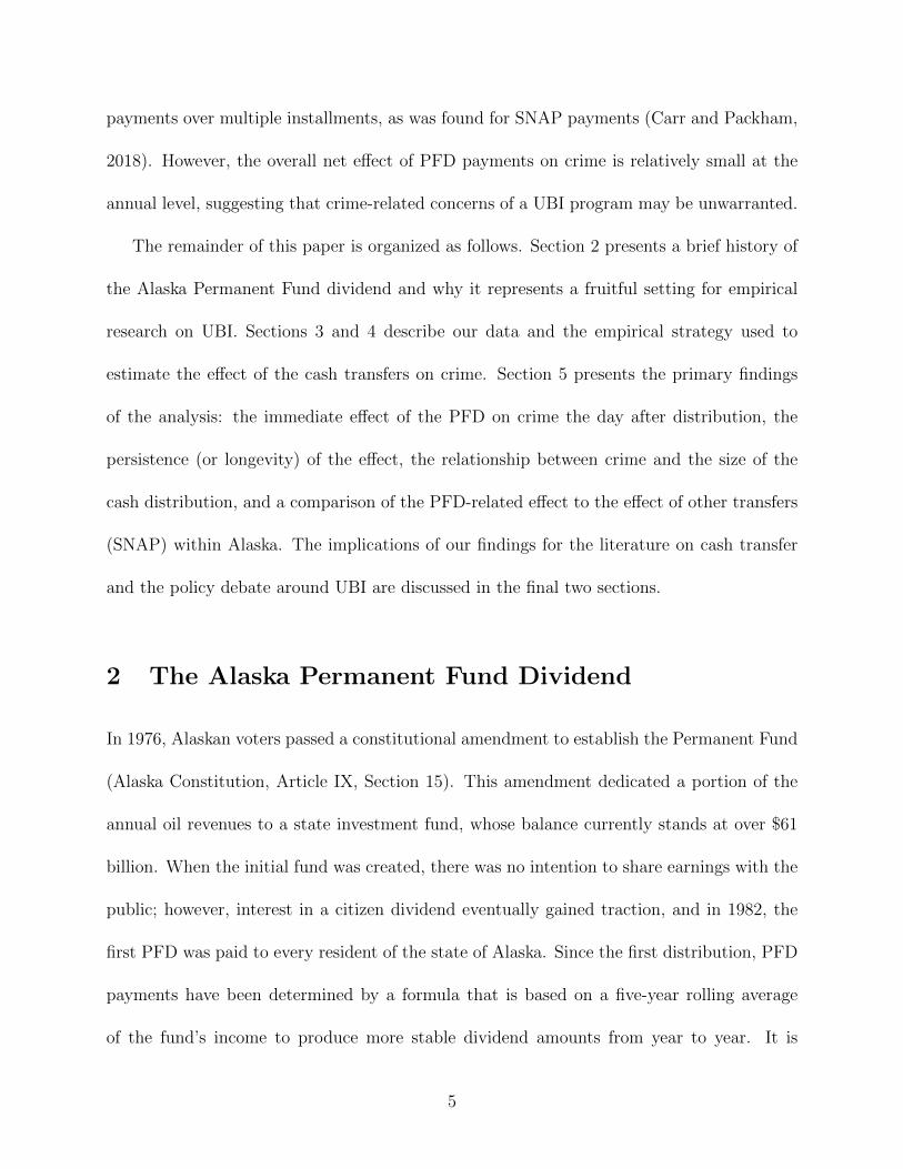
The remainder of this paper is organized as follows. Section 2 presents a brief history of

the Alaska Permanent Fund dividend and why it represents a fruitful setting for empirical

research on UBI. Sections 3 and 4 describe our data and the empirical strategy used to

estimate the effect of the cash transfers on crime. Section 5 presents the primary findings

of the analysis: the immediate effect of the PFD on crime the day after distribution, the

persistence (or longevity) of the effect, the relationship between crime and the size of the

cash distribution, and a comparison of the PFD-related effect to the effect of other transfers

(SNAP) within Alaska. The implications of our findings for the literature on cash transfer

and the policy debate around UBI are discussed in the final two sections.

2 The Alaska Permanent Fund Dividend

In 1976, Alaskan voters passed a constitutional amendment to establish the Permanent Fund

(Alaska Constitution, Article IX, Section 15). This amendment dedicated a portion of the

annual oil revenues to a state investment fund, whose balance currently stands at over $61

billion. When the initial fund was created, there was no intention to share earnings with the

public; however, interest in a citizen dividend eventually gained traction, and in 1982, the

first PFD was paid to every resident of the state of Alaska. Since the first distribution, PFD

payments have been determined by a formula that is based on a five-year rolling average

of the fund’s income to produce more stable dividend amounts from year to year. It is

5

important to note that the fund is well-diversified across different regions and asset classes;

thus, its returns are not necessarily reflective of Alaska’s economic conditions. State oil

revenue, which originally capitalized the fund, currently represent only 2-3% of annual fund

additions; since 1985 reinvestment of fund earnings is the primary way in which the fund

grows. The average annual aggregate distribution is large enough to be similar in size to

the Gross Domestic Product of many sectors in the Alaska economy. In 2015, for example,

the 976 million dollar distribution was about 42% of the construction sector’s GDP, or 76%

of the whole-trade sector’s. In addition to the sheer size, PFD payments are distributed to

everyone at the same time, which means it is the single largest infusion of money at a given

point in Alaska’s $50 billion economy.

As a case study in universal income, the dividend established an income floor below

which the cash income of residents cannot fall. This cash transfer is particular important in

rural areas where economies lack economic bases and are still a mixture of subsistence and

a small formal economy. Another key feature of the PFD is that amounts are not based on

a person’s income or wealth. Payments are uniformly distributed to all residents—adults

and children–of the state (including green-card holders and refugees) who were residents of

the state in the prior year. Over our study period (2000-2016), average household size was

2.83, average household income was $72,000, and average PFD size per-person was $1,600.

That means that the PFD represents, on average, 6.28% of overall household income. By

coincidence, this is almost exactly the share of earnings generated by the first PFD in 1982.

Since inception the program has become very popular and the public expects it to run in

perpetuity.

Each year the filing period runs from January 1st to March 31st. This leaves the Per-

6

manent Fund division about six months to process the applications, determine eligibility,

and handle garnishment requests. The payout month, therefore, is a result of administrative

processes, as opposed to any intentionality on the behalf of the founders of the dividend.

The vast of majority of Alaskans—82.72% as of 2014—receive their PFDs through direct

deposit in the first week of October, while the rest receive checks through the mail. Over

our study period (2000-2016), direct deposits have always been issued either before or on

the same day checks are mailed. More recently (since 2010), both direct deposits and checks

have been issued on the first Thursday of October. Because of the relatively small portion

of the population receiving mailed-checks, and because these checks are never issued before

direct deposits, our primary specifications focus on the first round of direct deposit issuance.

3 Data

We employ a database on reported policing incidents in Alaska’s largest city, the Municipality

of Anchorage. Limiting the study to Anchorage is not particularly narrow in scope, as the

city accounts for a large share (40%) of the state’s total population.1 The primary data for

the analysis are real-time incident reports for officers of the Anchorage Police Department

(APD). An incident report is generated each time an officer calls to report their location

and the nature of their current activity to dispatch. Such reports can be made, for example,

1In 2016, Anchorage’s population stood at just under 300,000, with another 150,000

in the larger metro area. Alaska as a whole recorded 750,000 residents in 2016.

Fairbanks, Alaska’s second largest city, has just 1/10 the population of Anchorage.

(www.census.gov/data/datasets/2016/demo/popest/total-cities-and-towns.html).

7

when an officer responds to a 911 call, initiates a traffic stop, services a warrant, or even

reports a meal break. Each time-stamped log entry is associated with a particular activity,

self-reported by the officer, and coded to one of 99 possible activities by the APD.

APD provided us with location de-identified incident reports for the years 2000-2016.

For our analysis, we aggregate these incident-report level data up to counts at the day level

for each activity code. Drawing from the categorization of the Federal Bureau of Investiga-

tion’s Uniform Crime Report (UCR) and with consultation from APD, we further categorize

and aggregate these specific codes to more general activity types corresponding to violence,

substance abuse, property crimes, noise violations and parties, and police department med-

ical assistance to other agencies. Our aggregation differs from UCR in three ways. First,

UCR reports robbery as a violent crime whereas we categorize it as a property crime (as

it is financially motivated). Second, UCR includes arson as a property crime, but because

it does not necessarily provide direct financial gain to the perpetrator, we omit it. Finally,

UCR does not track substance abuse incidents. Therefore, in consultation with APD, we

determined six incidents to be associated with substance abuse: hit-and-run events, liquor

law violations, problems with a drunk individual, police transportation of a drunk individual

(often for another city agency), drugs and forged prescriptions, and driving while intoxicated.

Hit-and-run violations have been shown to be associated with alcohol consumption (Solnick

and Hemenway, 1994). Liquor law violations tend to be associated with illegal possession

or sale of alcohol, rather than excessive consumption. For robustness, in Appendix tables,

we provide estimates for both an inclusive (Full) and restrictive (Part) categorization of

substance abuse incidents that differ by including hit-and-run and liquor law violations. As

these yield qualitatively similar results, the remainder of the paper only presents the results

8

for Substance (Full), which are inclusive of all incidents.

Appendix Table A.1 shows the average daily count of calls received over our sample period

for specific call codes and the more general categories to which they were assigned. Figure

A.1 shows these activities by day-of-week and month of year. Predictable weekday-weekend

and summer-winter patterns are visible in most of the series. For example, substance abuse

calls peak on the weekend, while property crime is low on the weekend as people are spending

time at home.

4 Empirical Strategy

Our empirical strategy exploits two sources of temporal variation to examine the PFD’s effect

on crime. First, we use the discrete intra-annual variation in the day the PFD is issued by

comparing daily behavioral outcomes from the days immediately following the PFD to similar

days of the year that do not experience cash transfers of any kind. Given that the time of

year in which the PFD is issued is determined only by administrative processes, the annual

timing of the PFD is exogenous;2 thus, similar days of the year that do not experience cash

transfers are plausible estimates of the counterfactual of what behavioral outcomes would

have been had the PFD not been issued. A useful feature of this source of variation is

that PFD payments have occurred on different days of the month and different days of the

week over the years in our sample. With variation in the day-of-the-month, the PFD can

be isolated from the effect of other income payments and transfers that occur on a regular

2This observation is based on personal communications with current and former govern-

ment officials involved in the creation of the PFD program.

9

schedule each and every month.3 With variation in the day-of-the-week, the PFD can be

separately identified from other regular weekly patterns, such as the effects of the weekend

versus the weekday. As a second source of variation, we use the inter-annual variation in the

size of the PFD payment to both provide additional identification and to explore whether

behavior is sensitive to the amount received. As previously discussed (Section 2), the size

of the PFD is determined based on the returns of a diversified portfolio rather than on

contemporaneous oil prices or specific factors related to the state economy. PFD payment

dates, number of recipients, and amounts are listed for each year in our study period in Table

1.

We estimate four different empirical model specifications to investigate different aspects

of the effect of the cash payment on daily criminal activity. First, we estimate an empirical

model that leverages the exogenous timing of the payment only:

yt = β0 + β1PFDt + γWt +Mt + τt + εt, (1)

3These transfers include food stamps and Temporary Assistance for Needy Families

(TANF), which are distributed on the first day of each month in Alaska; military pay-

checks, which are distributed on the 1st and 15th of each month (or the nearest busi-

ness day prior); and social security checks, which are distributed on the 2nd, 3rd, and

4th Wednesday of each month. Most salaries in the United States are paid weekly or

every other week (www.bls.gov/opub/btn/volume-3/how-frequently-do-private-businesses-

pay-workers.htm), creating day-of-the-week patterns in incomes, as opposed to day-of-the-

month-patterns.

10

where yt is the count of policing incidents on day t related to either violence, substance abuse,

property crime, noise/parties, or police medical assistance to other agencies (each estimated

separately); PFDt is a dummy variable taking a value of one if t equals the date of the

first PFD distribution and zero for all other days; and εt is the model error. The βi and γ

coefficients are parameters to be estimated. The coefficient of interest, β1, is the estimated

change in the number of incidents y on the first full day after PFD direct deposits are issued.4

We estimate Eq. 1 via OLS using heteroskedasticity- and autocorrelation-consistent Newey-

West estimates of the covariance matrix (Newey and West, 1987) to address any persistence

in the time series after accounting for month-by-year fixed effects.5

The specification in Eq. 1 includes a number of control variables and fixed effects.

Mt is a vector of month × year (month-by-year) fixed effects, which captures changes to

average incomes, unemployment, population, police department resources, and other similar

effects. Following the daily crime literature (e.g., Jacob and Lefgren, 2003; Foley, 2011), Wt

represents a vector of weather control variables (precipitation, maximum daily temperature,

and snow depth), which reduces observed variance and enables more precise estimates. Most

of the seasonal weather effects, however, are captured by the month-by-year fixed effects.

4For example, if the PFD is issued at sometime on Thursday, β1 will capture the effects

of PFDt from Friday at 12:00am to 11:59pm.5Poisson models were also fitted to address the count nature of the data, but yielded

similar results. These estimates are included in the Appendix Table A.4. We address test-

ing multiple hypotheses for our five outcome variables by using the Bonferroni correction

method. Less conservative corrections were also tested for our main results, but yielded

similar inference.

11

τt is a vector of special day, holiday, day-of-week, and day-of-month effects. Specifically,

τ includes day-of-week fixed effects (Monday, Tuesday, etc.), addressing weekend-versus-

weekday effects or intra-week cyclicality, and a 5th-order polynomial day-of-month trend

to account for events that occur on a regular monthly schedule, such as rental payments

and other income receipts (e.g. social security, food stamps, or other welfare receipt). τ also

includes a vector of special day dummy variables, including military pay days (to account for

the predictable pay of Anchorage’s large military population), New Year’s Eve/Day, Super

Bowl Sunday, the day of the Iditarod race start in Anchorage, St Patrick’s Day, Cinco de

Mayo, July 4th, Labor Day and Labor Day weekend, Columbus Day, Halloween/proceeding

weekend, Thanksgiving, Christmas Day, and federal holidays which are given to many public

employees if a major holiday falls on a weekend. Much like weather, including special date

indicator variables allows for more precise effect estimates by reducing the variance in the

counter-factual days.

In our second model specification, we investigate whether there is any persistence in the

PFD-effect beyond the first full day following the distribution by adopting an event-analysis

strategy similar to Evans and Moore (2011): we broaden the time window for the indicator

variable PFDt in Eq. 1 to one-week intervals, from four weeks before the PFD distribution

to four weeks after. Persistence of the PFD effect is estimated from Eq. 2,

yt = β0 +4∑

i=−4

βiPFDit + γWt + f(t) ∗ Y ear + τt + εt, (2)

where PFDit is a dummy variable taking a value of 1 if day t is in the ith week before/after

distribution and zero otherwise. We define weeks as the 7-day periods starting from the

12

day the PFD is distributed.6 Weather and holiday controls, W and τ , are defined as in

Eq. 1. The eight-week window around the PFD distribution date leaves relatively few

“untreated” October days to offer independent variation for estimating the monthly fixed

effect; instead, we use a 5th-order day-of-year polynomial trend, f(t), to capture seasonal

variation in the observed activity patterns through channels such as income, unemployment

and police department resources. We estimate such a trend for each year by interacting it

with a yearly fixed effect.

Assessing the persistence of the effect of the PFD on our outcomes allows us to determine

if the payment has a net cumulative impact or if the change in behavior immediately following

receipt merely represents an inter-temporal reallocation. In order to avoid conflating the

persistence of first-day recipients (who received PFD by direct deposit) with the effect of

new recipients who receive their PFDs later by check, we narrow our sample period for the

persistence estimates to the years 2010-2016, where direct deposits and checks were issued

to all recipients on the same day.7

An additional motivation for looking at an extended treatment period is that while the

first full day after the PFD distribution experiences particularly intense treatment, the one-

day treatment window may be too short to capture effects that are confined to particular

days of the week. For example, Mondays have the highest daily number of property crime

6In other words, the first week after distribution, i = 1, includes days 1-7 after distribu-

tion; days 8-14 correspond to week i = 2, and so on. The first seven days before the PFD

defines week i = −1; days 8-14 before the distribution defines week i = −2, and so on.7In most years in the 2000-2009 period, paper checks were mailed one week after direct

deposits were issued. For robustness, we also estimate Eq. 2 on the full sample (Table A.6).

13

calls, but no Monday falls the day after a PFD payment. This limits the potential impact

of the treatment effect to days that property crime might be otherwise depressed.

For our third empirical specification, we estimate the marginal response to the size of the

distribution, which additionally leverages the dollar amount paid as a source of identifica-

tion. As shown in Table 1, PFD amounts have varied considerably year-to-year, both in the

amount that each recipient is paid (between 918 and 3,644 2016 USD) and in the number

of individuals who receive their PFD as part of the first round of direct deposit payments.

Consequently, the total amount of cash hitting the street on the first day provides an oppor-

tunity to investigate how changes in the total size of the distribution relate to changes in our

estimated effects. These marginal effects are relevant for policy, as they potentially inform

potential gains from more evenly distributing payments over time (either across or among

individuals). To test for potential response to distribution size, we estimate the model in

Eq. 3,

yt = β0+β1weekPFDt +β2week

PFDt ×amountt+β3weekPFD

t ×amount2t +γWt+Mt+τt+εt, (3)

where weekPFDt is a dummy variable taking a value of one if t occurs during the week after

distribution and zero otherwise, and amountt is the total amount of cash dispersed on the

first day (PFD amount × number of first-day recipients) measured in 100 million 2016 USD

(Table 1). The other variables are defined as in Eq. 1. Main effects for amount are not

included because there is no intra-annual variation in the amount of the PFD payments or

first-day recipients; both will be perfectly correlated with month-by-year fixed effects.

Finally, to provide context for our PFD estimates, our fourth specification compares the

14

effect of the PFD to changes in police activity stemming from a transfer payment that has

been the focus in previous studies, food stamp (SNAP) payments. We single out the SNAP

program as it is an important social program which provides a predictable and steady stream

of benefits to income and asset-eligible households. SNAP has a large base of participation

and, unlike other programs like Temporary Assistance for Needy Families, payments do not

end after a given amount of time. Several previous studies have analyzed the short-run

effects of income or in-kind transfers using programs such as SNAP (e.g., Shapiro, 2005;

Cotti et al., 2016), or social security payments (e.g, Stephens, 2003; Mastrobuoni and Wein-

berg, 2009; Evans and Moore, 2011). Particularly relevant for our study, Foley (2011) and

Carr and Packham (2018) examine the relationship between crime and the timing of SNAP.

However, such transfer programs have important limitations when considering their implica-

tions for universal income. Social security payments are restricted to the elderly and SNAP

payments to those near or below the poverty level. Differing consumption patterns may be

expected from these sub-groups than for the population as a whole. Further, SNAP pro-

vides in-kind benefits which can only be spent on certain grocery items. Because universal

income is sometimes discussed as a substitute or complement for more traditional welfare

programs, comparing the behavioral responses of PFD receipt to those for such welfare pro-

grams provides insight into how these programs might differ. To our knowledge, no studies

to date have explored the differential effect of cash transfers on crime between universal and

non-universal transfer programs on a per-person basis.

For this comparison, we exploit both the discrete first-day-of-the-month timing for Alaskan

SNAP payments and the total size of these monthly distribution. The per-household SNAP

benefits in Alaska depend on the household size, income, and location (urban, rural, or

15

remote). Over our study period, statewide SNAP participation was approximately 65,000

individuals, or about 9.5% of the state’s population. On average, about $10 million is paid

in total benefits across the state each month, with an average per-person benefit of about

$150 per month. We compare SNAP to PFD through estimation of Eq. 4,

yt = β0+weekPFDt (β1+β2amount

PFDt )+weekSNAP

t (β3+β4amountSNAPt )+γWt+Mt+τt+εt

(4)

where weekPFDt is a dummy taking a value of 1 when day t falls in the week after PFD

distribution and zero otherwise, amountPFDt is the amount of PFD distributed as part of

the first direct deposit (in millions of 2016 USD) measured in deviations from the average

amount, weekSNAPt is a dummy taking a value of 1 when day t is in the week following

Alaskan SNAP distribution, and amountSNAPt are the SNAP payments made to Alaskans for

the month that t falls measured in deviations from their average.8 As before, W is a vector of

weather control variables, Mt is a vector of month-by-year effects, and τ is a vector of special

dates and day-of-week effects. For this specification, we drop the day-of-month polynomial

trend that captures intra-month cyclicality since we want to instead estimate this variation

as part of weekSNAP . The interactive effect of weekSNAPt × amountSNAP

t isolates the SNAP

payment from other first-of-the-month effects (e.g. other income receipt, rent payments, etc)

which would otherwise have the potential to confound identification. Further, an important

source of variation in amountSNAPt is driven by a temporary benefit increase enacted as part

of the American Recovery and Reinvestment Act of 2009 that was effective April 2009 to

8Data for the monthly SNAP distributions come from the the US Department of Agri-

culture’s State SNAP Tables.

16

November 2013 (Hastings and Shapiro, 2018). During this period, Alaska was only mildly

affected by the economic downturn facing the rest of the country as oil prices remained at

record highs. We estimate the marginal effect of th PFD for only the first week following

its distribution since payments to check recipients in 2000-2009 period conflate estimation

of persistence effect with the effect of new money being dispersed after the first week. The

week-long duration for estimating the SNAP effect is chosen based on a combination of the

existing literature (e.g., Cotti et al., 2016; Foley, 2011, which use relatively short durations

of ten days or less), empirical evidence from our data that suggests SNAP effects dissipate

after one week, simplicity, and symmetry to the PFD estimate.

5 Results

5.1 Day-After Effects of the PFD

The estimated results for Eq. 1 across the five incident-categories of interest are presented

in Table 2. The coefficient estimate for “First Full Day After PFD Deposit” represents

the change in the average number of daily incidents one day after the PFD distribution.

For reference, the daily mean and standard deviation for each outcome variable are also

presented in the table. For incidents related to substance abuse, there is an increase of

approximately six reported incidents after the first PFD direct deposit, an increase of 14.1%

over the daily sample average. This result is statistically significant even after correcting

for multiple hypotheses testing across our outcomes. We find no statistically significant

day-after effects in incidents of violence, property crime, or calls for medical assistance.

17

Incidents of loud parties and noise violations show about a 1-incident decrease. However, this

result is not robust to model specification or multiple hypothesis test corrections. Compared

to the holidays that we estimate as controls, the increase in same-day substance abuse

incidents from the PFD distribution is slightly larger than the increase on the 4th of July

and roughly half the increase on New Years Day/Eve, two holidays that are notorious for

excessive consumption of controlled substances.9

5.2 Persistence in the PFD Effect

Estimates of the PFD effect at each week interval, as well as their 95% confidence intervals,

using the 2010-2016 sample are presented in Figure 1.10 Daily substance-abuse incidents

9Table A.2 in the Appendix presents estimates of all holiday and other special days of

the year for reference. Appendix Table A.3 presents results with a more parsimonious set

of month-by-year and day-of-week controls (omitting the day-of-month polynomial, weather

controls, and special days); these results yield the same inferences with the exception of party

and noise noted above. Appendix Table A.7 presents results for two sub-sample periods,

2000-2009 and 2010-2016; the latter sub-sample is used in the persistence analysis. The

effect magnitudes across outcomes are roughly equivalent over these two periods.10Table A.6 presents the tabular results. Daily-level persistence estimates are presented

in Figure A.2. Table A.6 also presents results estimated on the full 2000-2016 sample period

as a check for sensitivity to the sample period. In the full sample, property crimes see

statistically significant reductions for four weeks after the first direct deposit. In contrast,

these reductions are statistically significant for only two weeks in the 2010-2016 sample. This

result is consistent with our reasoning for narrowing the sample: the longer-lived reductions

18

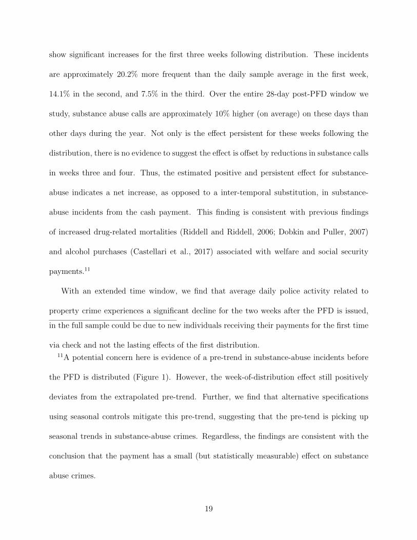
show significant increases for the first three weeks following distribution. These incidents

are approximately 20.2% more frequent than the daily sample average in the first week,

14.1% in the second, and 7.5% in the third. Over the entire 28-day post-PFD window we

study, substance abuse calls are approximately 10% higher (on average) on these days than

other days during the year. Not only is the effect persistent for these weeks following the

distribution, there is no evidence to suggest the effect is offset by reductions in substance calls

in weeks three and four. Thus, the estimated positive and persistent effect for substance-

abuse indicates a net increase, as opposed to a inter-temporal substitution, in substance-

abuse incidents from the cash payment. This finding is consistent with previous findings

of increased drug-related mortalities (Riddell and Riddell, 2006; Dobkin and Puller, 2007)

and alcohol purchases (Castellari et al., 2017) associated with welfare and social security

payments.11

With an extended time window, we find that average daily police activity related to

property crime experiences a significant decline for the two weeks after the PFD is issued,

in the full sample could be due to new individuals receiving their payments for the first time

via check and not the lasting effects of the first distribution.11A potential concern here is evidence of a pre-trend in substance-abuse incidents before

the PFD is distributed (Figure 1). However, the week-of-distribution effect still positively

deviates from the extrapolated pre-trend. Further, we find that alternative specifications

using seasonal controls mitigate this pre-trend, suggesting that the pre-tend is picking up

seasonal trends in substance-abuse crimes. Regardless, the findings are consistent with the

conclusion that the payment has a small (but statistically measurable) effect on substance

abuse crimes.

19

with an average daily decrease of 15.2% and 10.3% in the first and second week after payment,

respectively. The significant week-after effect is largely driven by decreased activities during

days that experience above-average property crimes (i.e., Monday to Wednesday). Like

incidents of substance-abuse, this effect is not offset in the later periods, indicating a net

decline in property crime, which is consistent with past findings of declines in property crime

associated with the timing of benefit payments (Carr and Packham, 2018; Foley, 2011) and

improvements in economic conditions more generally (Lin, 2008; Gould et al., 2002; Bignon

et al., 2017). Further, these reductions imply that the income effect dominates the potential

“loot” effect of a cash transfer, at least over the examined time horizon. Over the full 28-day

post-PFD window, the average daily reduction in property crime is 8%.

Like property crime, medical assistance from the Anchorage Police Department also shows

response in the extended time period not seen on the first full day after payment (Table 2).

Specifically, we observe a 9% increase in the 28-day post-PFD window. Note however that

these requests do not represent the universe of 911 calls regarding medical emergencies. They

only represent requests for medical assistance from police from other city agencies.

5.3 Variation in the Size of the PFD

From Eq. 3, the marginal effect of an additional $100 million in first-day cash from the

PFD is β2 + 2 × β3 ×Amount. We evaluate the marginal effect at the sample average PFD

dispersement, which is approximately $697 million in 2016 dollars (Table 3). For a $100

million dollar increase in the PFD (14% above the average distribution), the number of

calls requesting police to assist with medical issues increases by 0.35 calls per day (about

20

a 2% increase relative to the daily sample average). In addition, substance-abuse incidents

experience approximately a one incident-per-day increase, or a 2% increase over the daily

sample average, indicating an elasticity of 0.14, which is consistent with the finding that

alcohol is a normal good.12 While a variety of factors could explain the higher substance

abuse incidents with higher PFD payments, our findings are consistent with the finding that

cash aid creates “full wallets” that can exacerbate substance abuse problems (Dobkin and

Puller, 2007).

Despite the existence of a negative average effect on property crimes, the marginal ef-

fect of the size of the PFD is not statistically significant. A few different explanations are

possible for why higher distribution amounts do not result in further reductions in property

crime. First, based on the figures we cite in Table 1, it is possible that the annual fluc-

tuations in the PFD are not large enough to cause additional decreases in property crime

activity. Second, it’s possible that the PFD amounts observed in our sample identify a region

of the income/property-crime relationship where there are diminishing returns to income.

For instance, Loughran et al. (2013) find that the illegal wage rate among individuals who

engage in criminal activity is $929 per week, which is approximately equal to the lowest

12Although Evans and Popova (2017) present evidence from across the world that cash

transfers are not consistently used for alcohol or tobacco, evidence from the United States,

suggests that alcohol is a normal good Decker and Schwartz (2000). Dasso et al. (2014) also

refer to alcohol as a “temptation good”, a term used by Banerjee and Mullainathan (2010)

to refer to “goods that generate positive utility for the self that consumes them, but not for

any previous self that anticipates that they will be consumed in the future.”

21

per-person PFD received over the years in our sample (Table 1).13 Thus, fluctuations in the

amount distributed may not reduce the number of property crimes given that the smallest

PFD amount is almost as high as the earnings a skilled criminal can earn in a week. This

potential explanation is consistent with Mocan and Bali (2010), who evaluate the effect of

unemployment on crime and find that most of the impact of unemployment is observed in

pulling people into crime, rather than increasing the number of crimes of those who are

already committing crimes. Finally, it is possible that the loot effect at higher PFD amounts

offsets any additional income effect.

Altogether, the estimated marginal effects have two important implications. First, they

provide support for our earlier results as they use additional exogenous variation to further

isolate the PFD from any early-October effects. Second, since the socially undesirable out-

comes of substance abuse and medical-assist instances are increasing in distribution size, but

the socially desirable outcome of reduced property crime is not, there are implied gains from

spreading the payments over the year.

13Loughran et al. (2013) also note that there is considerable skew in the data (s.d. =

$1,491). A recent paper by Nguyen and Loughran (2017) reaches a similar conclusion that

the distributions of self-report criminal activity are asymmetric and right-skewed, with long

right tails. In one sample, they find average weekly criminal wage of $1,470 (median $669),

whereas in the other sample the reported average weekly criminal wage was $914 (median

$316).

22

5.4 Comparison to Non-universal/In-kind Payments

In this section, we compare our estimated effects to those for a particular non-universal,

in-kind transfer receipt, food stamps (SNAP). As previously discussed, SNAP and the PFD

differ in two important respects. First, the universal nature of the PFD makes the average

PFD recipient quite different than the average SNAP recipient. This is true with respect

to both income (by definition) and across other sociodemographic dimensions. While Grant

and Dawson (1996) provide evidence that the welfare receiving population does not system-

atically differ from non-receivers in their alcohol abuse, Pollack and Reuter (2006) find that

drug usage was higher among welfare-receiving individuals. Further, Hastings and Wash-

ington (2010) show that alcohol and tobacco purchases for SNAP recipients (relative to

non-recipients) are highest soon after SNAP receipt. For these reasons, we would expect

substance-abuse crimes to be more elastic with respect to SNAP payments than PFD pay-

ments. The second difference between SNAP and the PFD is the in-kind (or conditional)

nature of the SNAP payments. SNAP recipients may spend food stamps disproportionately

on eligible food items relative to other sources of income: thus, substance-abuse incidents

may be more elastic with respect to unrestricted payments like the PFD.14

Table 4 displays the estimated coefficients of interest from Eq. 4. The main effects

suggest that substance-abuse incidents are more frequent during the week in which SNAP

payments are distributed while property crime incidents are lower the week after the PFD

14Cuffey et al. (2016) in a survey/meta-analysis of fifty-nine papers and Hastings and

Shapiro (2018) both find notable gap between the marginal propensity to purchase eligible

food from food stamps than from other income.

23

is distributed. We note, however, that this only suggestive as the main effect estimates for

SNAP (SNAPWeek) are not separately identified from other first-of-the-month occurrences,

although our estimates for reductions in property crime is not dramatically different from

Foley (2011).15 Similarly, Dobkin and Puller (2007) find an increase in hospital admissions

related to drug abuse during the first few days of the month attributable to receipt of

supplemental security income programs (SSI). While their results are consistent with the

results we find for medical assistance and substance abuse incidents, we note that SSI is

issued as a cash transfer while SNAP benefits are in-kind benefits.

Turning to the marginal effect estimates, an increase of $1 million in the size of the

monthly SNAP distribution is associated with a statistically significant increase of 0.46 in

the average number of daily substance abuse incidents over the first week, compared to an

increase of only 0.002 daily substance abuse incidents in the first week from a $1 million

increase in the size of the PFD distribution. Medical assistance incidents are also responsive

to the distribution sizes of both payments, with an additional $1 million resulting in 0.001

and 0.064 increase in calls for the PFD and SNAP, respectively. Given the different scales of

the PFD and SNAP programs, the lower panel of Table 4 facilitates the comparison of these

two programs by presenting the marginal effects in elasticity terms and tests the hypothesis

that the difference in crime-payment elasticities for SNAP versus the PFD is statistically

different from zero. We find such a difference in response of substance abuse to payment

15Foley (2011) finds property crime to be 3.8% lower in the first 10 days after SNAP

distribution; we find a 2.5% decrease. While our results are somewhat smaller, this is intuitive

considering that Anchorage has a lower participation rate in SNAP that the average city in

Foley’s study (which were sampled based on high participation rates in the program).

24

receipt, but not for the other categories of activities.

The goal of comparing SNAP- to PFD-related effects is to highlight the differential effects

of universal cash payments relative to those previously studied for non-universal and in-kind

payments. The more responsive nature of substance-abuse crimes with respect to SNAP

payments suggests that the universal nature of the PFD more than offsets any relative

difference arising from the unconditional nature of the PFD, as per the discussion above.

However, we note that there are several other potential explanations for why substance-abuse

incidents are relatively more responsive to SNAP payments. PFD and SNAP payments are

quite different in size, and the effect that we are trying to estimate may be highly non-

linear—e.g., a $150 SNAP payment leads to increases in crime, while a $1,000 PFD payment

does not. In addition, the scale of the PFD program has the potential to induce general

equilibrium effects and create demand for labor (as found by Jones and Marinescu, 2018),

which could attenuate the crime response from the PFD payments.

5.5 Robustness of findings

To further scrutinize our findings, we test whether similarly sized effects for the PFD can be

found during other one-week periods of the year. For this test, we estimate Eq. 1 iteratively,

redefining treatment for a new week-of-year at each step. Placebo treatment weeks are

defined starting at the true treatment week and working outward within each year. Because

of this definition, the weeks at the beginning and end of each year will not necessarily contain

seven days. Also, as the number of weeks before and after the true dispersement week varies

from year to year, we will estimate more than 52 placebo effects. Figure 2 plots a histogram

25

of the magnitude of these placebo treatment effects for each outcome, along with the fraction

of observed effects that are greater in magnitude than the actual treatment. The results of

the placebo test are consistent with the those presented in the main results tables. Substance

abuse and property crime are both found to have true treatments in the 10th percentile of all

estimated effects. Placebo effects for these outcomes of similar or larger magnitude are also

easily explained by spillovers from holidays or log accounting issues from daylight savings

time.

A potential threat to identification is a change in the level of police enforcement activity

around the time of PFD distribution: if APD anticipates a swell in activity around the time

of the distribution, it may increase its presence and observe more crime taking place (whether

the actual underlying level changes or not). Our conversations with the APD suggest that

staffing effort does not change around the time of PFD distribution. Further, most of the

activities of interest in our analysis are so-called “calls for service”. Calls for service are

initiated by members of the community (e.g., calling 911, hailing officer in the field, or

request by other agency), in contrast to “self-initiated” activities which are more responsive

to changing enforcement. In Appendix C we find no evidence that the total number of

calls for service, self-initiated activities, or their their ratio change on PFD distribution day,

relative to other days. This is in contrast to periods and holidays with known enforcement

changes.

26

6 Discussion

Our analysis finds an increase in the number of substance-abuse incidents and a decrease in

the number of property crimes in the weeks immediately following the PFD distribution; a

remaining question is whether such changes can be considered as economically significant.

Estimates of the persistence of the PFD effect (Figure 1 and Table A.6) indicate that 126

more substance-abuse incidents and 77 fewer property crimes are realized over the four weeks

after the PFD is distributed, on average. On an annual basis, this constitutes only a 1.05%

increase and 0.61% decreases in substance-abuse incidents and property crimes, respectively

(Table 5). Further, many of the substance-abuse incidents that are attributable to the PFD

constitute crimes that may not be overly costly to society. For example, decomposing the

substance-abuse category into its individual components indicates that our substance-abuse

results are being driven by increases in crimes such as “drunk problem” and “drunk trans-

port” (See Appendix Table A.5). To understand the potential cost of such crimes, we com-

pute estimates of the costs associated with the increase in alcohol-related crimes and compare

them to the cost savings associated with the reduction in property crimes (see Appendix B

for more detail). We provide a low-cost case, which assumes the cost of crime includes only

tangible costs and a high-cost case, which assumes that the cost of crime includes tangible

and intangible costs.16 The high cost case also incorporates the probability that substance

16From McCollister et al. (2010), tangible costs include the victim’s economic loss (medical

costs, lost earnings, and property loss), criminal justice cost, and the opportunity cost for

the criminal from foregone legitimate pursuits. In contrast, intangible costs incorporate pain

and suffering.

27

consumption induces additional crime.17 Our back-of-the-envelope calculation suggests that

the cost of increased alcohol-related incidents ranges between $4.5 thousand and $3.9 million

over the four weeks after the distribution, depending on whether both direct and indirect

costs of alcohol-related crimes are included in the calculation and whether the costs include

intangibles. In contrast, we estimate the cost savings from the decrease in property crimes

to be between $333 thousand and $419 thousand. Together, these estimates suggest that the

net effect of crime attributable to the PDF lies between +$329 thousand and -$3.4 million

(Table 5). While the sign of the estimated net welfare effect depends on our assumptions

about which costs to include, we interpret the economic significance of the welfare effect

as unambiguously small. In comparison to the size of the total PFD payment received by

Anchorage residents, for instance, the welfare changes associated with crime range from a

0.17% savings to a 1.78% loss across the low and high cost cases. In per capita terms, these

changes are between a $1.54 per person savings to a $16.12 loss, relative to 2016 per-person

PFD amount of $1,022.

Despite the relatively small calculated welfare impact, there may be potential to reduce

the impact of PFD-related crime by restructuring the timing of the PFD. For instance, our

results suggest that substance-abuse incidents increase with the size of the PFD, but no

further reductions in property crimes occur. This implies that there may be benefits to

staggering the PFD payments over the year: smaller amounts may reduce the negative “full

17Alcohol-related crimes have direct costs (e.g., police resources to manage disorderly

individuals, as in Rajkumar and French, 1997), but also indirect costs via an increased

likelihood of committing other crimes while under-the-influence (e.g., the alcohol-violence

link shown by Lindo et al., 2018).

28

wallet” effect without increasing financially motivated crimes. However, as the size of our

results are small, any gains from reducing substance-abuse incidences should be weighted

against any administrative costs associated with issuing multiple payments a year. In ad-

dition, the relationship between payment size and property crimes is not well-identified for

smaller payments that lie outside of our observed sample of historical PFD payments; thus,

several small payments may not have the same effect on property crime as we estimate in

our analysis. Nevertheless, our findings are consistent with a number of recent papers on

conditional cash transfers showing gains from staggering payments (Dobkin and Puller, 2007;

Carr and Packham, 2018). The gains in our case, however, are smaller due to the universal

nature of the payment and the difference in the treated population. While the deviations

we find are small on an annualized basis, they do suggest that future implementations of

universal income should test alternative disbursement policies that maximize the reductions

of financially motivated crimes while reducing substance-abuse activity, which can result in

crime.

7 Conclusion

We present the first comprehensive analysis of the crime consequences of an unconditional

and universal transfer using the world’s only continuous universal income program, Alaska’s

Permanent Fund Dividend. Our findings provide several new insights for the impact of cash

transfers on the behavior of recipients. We show that the recipient population is responsive

to an unconditional and anticipated income receipt across several dimensions of interest.

Over the four week period after the PFD distribution, we find an average daily reduction in

29

property crime of 8%, an average daily increase in substance abuse crime of 10%, and an

average daily increase in medical assistance calls of 9%. Our substance abuse results confirm

the mechanisms underlying previous work that finds increases in substance-abuse-related

morbidity and mortality following cash transfers from SSI and welfare programs (Dobkin

and Puller, 2007; Riddell and Riddell, 2006). However, our results stand in contrast to other

work that finds more limited, or even negative, substance-abuse-related responses to cash

transfers (Cuffey et al., 2016). Additionally, we find substance abuse and medical calls for

assistance are responsive to the total size of the payment program (in terms of dollars) but

property crimes are not. Our property crime results, in general, support previous work that

finds a decrease in property crime following SNAP payments in twelve US cities (Foley,

2011). The observed changes we describe above are, however, modest as the increase in

substance-abuse crime is 1.05% of the annual level, while the declines in property crime are

-0.61%.

Our results also contribute a new dimension to the growing literature on universal basic

income. We show the potential for such programs to produce both positive and negative

social consequences. On the negative side, we show that unconditional cash transfers do

in fact increase recipient’s consumption of “temptation goods,” or controlled substances (as

measured by policing activities). On the positive side, we show that a universal cash trans-

fer also decreases property crime. These positive and negative effects are quite different in

magnitude (on a per dollar/per person basis) than the estimated effects of other transfers

which have been the subject of past work. In our analysis, when the PFD and food stamp

(SNAP) program are compared, we find that the SNAP-distribution elasticity of substance

abuse calls is over four times larger than that of the PFD. The results of this comparison

30

provide quantitative evidence regarding the fundamentally different nature of universal pay-

ments from payments such as food stamps or social security that have been the subject

of many past studies. As such, generalizing the findings of conditional, non-universal, and

in-kind transfer literature to more universal payments may be problematic due to the differ-

ences in the average recipient’s response. Indeed, the small estimated crime-related costs of

the PFD suggest that crime-related concerns of a universal cash transfer program may be

unwarranted.

Finally, we show that lessons from the PFD can potentially be very useful in understand-

ing the consequences associated with UBI implementations. Our focus in this paper has

been on a subset of behavioral responses (i.e., criminal activity) as measured by daily police

activity records. Clearly, the goals of UBI have far reaches and some are beyond the scope of

this paper. The length of time the PFD has been in existence provides a unique opportunity

for researchers to investigate, the health, education, labor, and other social effects on the

Alaska population.

31

References

Banerjee, A. and S. Mullainathan (2010, 5). The Shape of Temptation: Implications for the

Economic Lives of the Poor.

Becker, G. S. (1968, 3). Crime and Punishment: An Economic Approach. Journal of Political

Economy 76 (2), 169–217.

Bignon, V., E. Caroli, and R. Galbiati (2017). Stealing to Survive? Crime and Income

Shocks in Nineteenth Century France. Economic Journal .

Billings, S. B., D. J. Deming, and S. L. Ross (2016). Partners in Crime: Schools, Neighbor-

hoods and the Formation of Criminal Networks. NBER Working Paper Series 21962.

Blakeslee, D. S. and R. Fishman (2018, 7). Weather Shocks, Agriculture, and Crime. Journal

of Human Resources 53 (3), 750–782.

Borraz, F. and I. Munyo (2014). Conditional Cash Transfers and Crime: Higher Income but

also Better Loot.

Carr, J. B. and A. Packham (2018). SNAP Benefits and Crime: Evidence from Changing

Disbursement Schedules. Review of Economics and Statistics , Forthcoming.

Castellari, E., C. Cotti, J. Gordanier, and O. Ozturk (2017). Does the Timing of Food

Stamp Distribution Matter? A Panel-Data Analysis of Monthly Purchasing Patterns of

US Households. Health Economics 26, 1380–1393.

Chioda, L., J. M. P. De Mello, and R. R. Soares (2016). Spillovers from conditional cash

transfer programs: Bolsa Familia and crime in urban Brazil. Economics of Education

Review 54, 306–320.

Cotti, C., J. Gordanier, and O. Ozturk (2016, 11). Eat (and Drink) Better Tonight: Food

32

Stamp Benefit Timing and Drunk Driving Fatalities. American Journal of Health Eco-

nomics 2 (4), 511–534.

Cuffey, J., T. K. Beatty, and L. Harnack (2016, 12). The potential impact of Supplemental

Nutrition Assistance Program (SNAP) restrictions on expenditures: a systematic review.

Public Health Nutrition 19 (17), 3216–3231.

Damm, A. P. and C. Dustmann (2014, 6). Does Growing Up in a High Crime Neighborhood

Affect Youth Criminal Behavior? American Economic Review 104 (6), 1806–1832.

Dasso, R., F. Fernandez, J. Aguero, E. Conover, G. Fack, C. Lopez, A. Tarozzi, J. Valder-

rama, F. Barrera-Osorio, M. Barron, C. Calvo, M. Angel Carpio, C. Lehmann, E. Naka-

sone, A. Sanchez, and N. Schady and (2014). Temptation Goods and Conditional Cash

Transfers in Peru. Technical report.

Decker, S. L. and A. E. Schwartz (2000). Cigarettes and Alcohol: Substitutes or Comple-

ments?

Dobkin, C. and S. L. Puller (2007, 12). The effects of government transfers on monthly

cycles in drug abuse, hospitalization and mortality. Journal of Public Economics 91 (11-

12), 2137–2157.

Evans, D. K. and A. Popova (2014). Cash Transfers and Temptation Goods: a Review of

Global Evidence. The World Bank Policy Research Working Paper May(6886), 1–3.

Evans, D. K. and A. Popova (2017). Cash Transfers and Temptation Goods. Economic

Development and Cultural Change.

Evans, W. N. and T. J. Moore (2011, 12). The short-term mortality consequences of income

receipt. Journal of Public Economics 95 (11-12), 1410–1424.

Foley, C. F. (2011, 2). Welfare Payments and Crime. Review of Economics and Statis-

33

tics 93 (1), 97–112.

Gould, E. D., B. A. Weinberg, and D. B. Mustard (2002). Crime rates and local labor market

opportunities in the United States: 1979-1997.

Grant, B. F. and D. A. Dawson (1996, 10). Alcohol and drug use, abuse, and dependence

among welfare recipients. American Journal of Public Health 86 (10), 1450–4.

Hastings, J. and J. M. Shapiro (2018). How Are SNAP Benefits Spent? Evidence from a

Retail Panel . American Economic Review 108 (12), 3493–3540.

Hastings, J. and E. Washington (2010). The First of the Month Effect: Consumer Behavior

and Store Responses. American Economic Journal: Economic Policy 2, 142–162.

Jacob, B. A. and L. Lefgren (2003, 11). Are Idle Hands the Devils Workshop? Incapacitation,

Concentration, and Juvenile Crime. American Economic Review 93 (5), 1560–1577.

Jones, D. and I. E. Marinescu (2018, 2). The Labor Market Impacts of Universal and

Permanent Cash Transfers: Evidence from the Alaska Permanent Fund. Working Paper

24312. National Bureau of Economic Research.

Kueng, L. (2018, 11). Excess Sensitivity of High-Income Consumers. The Quarterly Journal

of Economics 133 (4), 1693–1751.

Lin, M.-J. (2008). Does Unemployment Increase Crime? Journal of Human Resources 43 (2),

413–436.

Lindo, J. M., P. Siminski, and I. D. Swensen (2018). College Party Culture and Sexual

Assault. American Economic Journal: Applied Economics 10 (1), 236–265.

Loughran, T. A., H. Nguyen, A. R. Piquero, and J. Fagan (2013). The Returns to Criminal

Capital. American Sociological Review .

Machin, S. and C. Meghir (2004, 10). Crime and Economic Incentives. Journal of Human

34

Resources XXXIX (4), 958–979.

Marinescu, I. (2017). No Strings Attached: The Behavioral Effects of U.S. Unconditional

Cash Transfer Programs. Technical report, Roosevelt Institute.

Mastrobuoni, G. and M. Weinberg (2009, 7). Heterogeneity in Intra-Monthly Consumption

Patterns, Self-Control, and Savings at Retirement. American Economic Journal: Eco-

nomic Policy 1 (2), 163–189.

McCollister, K. E., M. T. French, and H. Fang (2010). The cost of crime to society: New

crime-specific estimates for policy and program evaluation. Drug and Alcohol Dependence.

Mejia, D. and A. Camacho (2013). The externalities of conditional cash transfer programs

on crime: the case of Bogota’s familias en accion program. Lacea 2013 Annual Meeting .

Mocan, H. N. and T. G. Bali (2010). Asymmetric crime cycles. Review of Economics and

Statistics .

Newey, W. K. and K. D. West (1987, 5). A Simple, Positive Semi-Definite, Heteroskedasticity

and Autocorrelation Consistent Covariance Matrix. Econometrica 55 (3), 703.

Nguyen, H. and T. A. Loughran (2017). On the reliability and validity of self-reported illegal

earnings: implications for the study of criminal achievement. Criminology .

Pollack, H. A. and P. Reuter (2006, 11). Welfare receipt and substance-abuse treatment

among low-income mothers: the impact of welfare reform. American Journal of Public

Health 96 (11), 2024–31.

Rajkumar, A. S. and M. T. French (1997). Drug abuse, crime costs, and the economic

benefits of treatment. Journal of Quantitative Criminology .

Riddell, C. and R. Riddell (2006). Welfare Checks, Drug Consumption, and Health: Evidence

from Vancouver Injection Drug Users. The Journal of Human Resources 41 (1), 138–161.

35

Shapiro, J. M. (2005, 2). Is there a daily discount rate? Evidence from the food stamp

nutrition cycle. Journal of Public Economics 89 (2-3), 303–325.

Solnick, S. J. and D. Hemenway (1994, 11). Hit the bottle and run: the role of alcohol in

hit-and-run pedestrian fatalities. Journal of Studies on Alcohol 55 (6), 679–684.

Stephens, M. (2003). “3rd of tha Month”: Do Social Security Recipients Smooth Consump-

tion between Checks? The American Economic Review 93 (1), 406–422.

Stephens, M. and T. Unayama (2011). The Consumption Response to Seasonal Income:

Evidence from Japanese Public Pension Benefits. American Economic Journal: Applied

Economics 3, 86–118.

Thigpen, D. E. (2016). Universal Income: What Is It, and Is It Right for the U.S.? Technical

report, Roosevelt Institute.

White, J. S. and S. Basu (2016). Does the benefits schedule of cash assistance programs affect

the purchase of temptation goods? Evidence from Peru. Journal of Health Economics .

Wright, R., E. Tekin, V. Topalli, C. McClellan, T. Dickinson, and R. Rosenfeld (2017, 5).

Less Cash, Less Crime: Evidence from the Electronic Benefit Transfer Program. The

Journal of Law and Economics 60 (2), 361–383.

36

8 Tables and Figures

Table 1: PFD direct deposit dates, number of deposits, and amounts (2000-2016)

Year

Direct

Deposit

Date

Day

of

Week

Number

of Direct

Deposits

%

Fulla

PFD

Amount

per person

(’16 USD)

% Deposits

Received

First Day

Total cash

dispersed

first day

(million

’16 USD)

2000 4-Oct Wed 390,312 96% 2,737 100% 1,030

2001 10-Oct Wed 404,247 96% 2,508 100% 970

2002 9-Oct Wed 424,490 97% 2,056 100% 844

2003 8-Oct Wed 444,268 94% 1,445 100% 605

2004 12-Oct Tue 448,642 94% 1,169 100% 491

2005 12-Oct Wed 459,004 94% 1,039 100% 448

2006 4-Oct Wed 476,775 93% 1,318 39% 227

2007 3-Oct Wed 493,997 93% 1,915 45% 395

2008 12-Sep Fri 497,739 92% 3,644 100% 1,670

2009 8-Oct Thu 514,217 93% 1,460 100% 702

2010 7-Oct Thu 527,868 92% 1,410 100% 684

2011 6-Oct Thu 523,756 91% 1,253 100% 594

2012 4-Oct Thu 518,334 90% 918 100% 429

37

2013 3-Oct Thu 512,955 89% 927 100% 426

2014 2-Oct Thu 518,986 88% 1,910 100% 874

2015 1-Oct Thu 532,672 87% 2,098 100% 976

2016 6-Oct Thu 534,156 89% 1,022 100% 484

Mean 483,672 92% 1,966 93% 697

PFD dates, number of recipients, and amounts come from Alaska Department of

Revenue’s Permanent Fund Dividend Annual reports. Total dispersed on first day

(in 2016 USD) are author’s calculations based on fully untarnished payments made

to recipients on the first payout date.

aThe fraction of ungarnished payments issued. Garnishments may be involuntary

(e.g. child support or uncollected government fees) or voluntary (e.g. tax exempt

college savings or charitable contribution).

Table 2: Change in reported incidents, first day after PFD distribution, 2000-2016

Change in daily incident count by category:

Violence Substance Property Party Medical

Assist

(1) (2) (3) (4) (5)

First Full Day −0.087 6.163∗∗∗ −0.656 −1.022∗ 0.914

After PFD Deposit (0.948) (1.964) (1.504) (0.603) (0.885)

P-value [0.927] [0.002] [0.663] [0.090] [0.302]

38

Bonferroni P-val [1.0000] [0.0086] [1.0000] [0.4498] [1.0000]

Mean Daily Call Count 13.63 43.59 33.70 10.08 14.38

St. dev Call Count 4.46 13.45 9.46 6.68 5.70

Weather Yes Yes Yes Yes Yes

Holiday Effects Yes Yes Yes Yes Yes

Day of Week Fixed Effects Yes Yes Yes Yes Yes

Day-of-Month Poly. Trend Yes Yes Yes Yes Yes

Month x Year Effects Yes Yes Yes Yes Yes

Observations 6,193 6,193 6,193 6,193 6,193

Adjusted R2 0.092 0.602 0.482 0.693 0.516

Note: Newey-West Robust Errors in parentheses. Unadjusted p-values: ∗p<0.1;

∗∗p<0.05; ∗∗∗p<0.01

Violence includes: Homicide, assault, and sexual assault. Substance category includes:

incidents of driving while intoxicated, drunk and disorderly, drug possession, hit-and-

runs, and liquor law violations. Property crime includes burglary, robbery, theft, and

shoplifting. Party includes noise violation and loud/disruptive party calls. Medical

assistance calls only include police assistance of medical aid for another department.

Complete list of holidays accompanies discussion of Eq. 1. Weather includes third order

effects for temperature, precipitation, and snow depth. Bonferroni p-values correct for

multiple hypothesis testing.

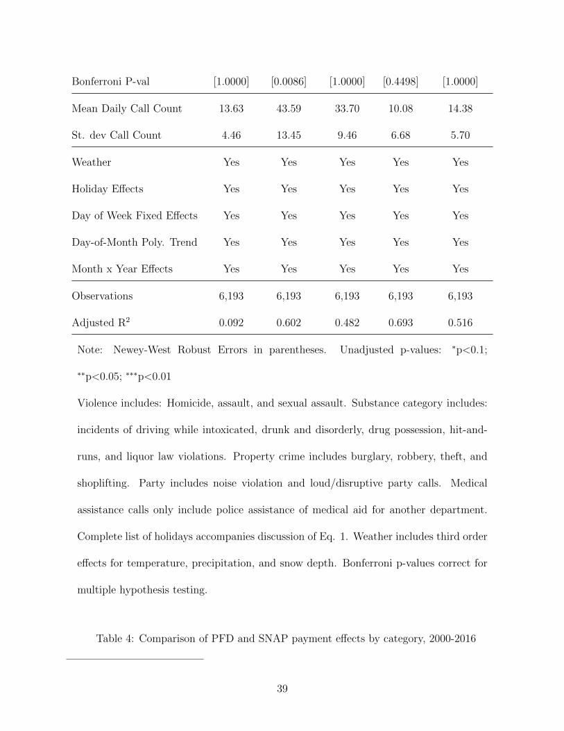
Table 4: Comparison of PFD and SNAP payment effects by category, 2000-2016

39

Dependent variable:

Violence Substance Property Party Medical

Assist

(1) (2) (3) (4) (5)

SNAP Week 0.121 5.298∗∗∗ −0.834∗∗∗ −0.132 0.702∗∗∗

(0.130) (0.376) (0.230) (0.118) (0.136)

PFD Week −0.283 3.133∗∗ −2.890∗∗∗ −0.150 0.660∗∗

(0.415) (1.243) (0.652) (0.299) (0.332)

SNAP Week x 0.033 0.462∗∗∗ −0.016 0.019 0.064∗∗

SNAP Amount (0.032) (0.099) (0.053) (0.027) (0.031)

PFD Week x 0.001 0.002∗ 0.001 −0.001∗∗ 0.001∗∗∗

PFD Amount (0.001) (0.001) (0.001) (0.0004) (0.0003)

SNAP Elasticity 0.026 0.117 -0.005 0.021 0.049

PFD Elasticity 0.027 0.038 0.012 -0.050 0.051

SNAP-PFD Elasticity -0.000 0.079 -0.017 0.071 -0.002

F-test P-value [0.990] [0.013] [0.440] [0.062] [0.942]

Bonferroni P-value [1.000] [0.066] [1.000] [0.249] [1.000]

Weather Yes Yes Yes Yes Yes

Holiday Yes Yes Yes Yes Yes

Day of Week Fixed Effects Yes Yes Yes Yes Yes

Day-of-Month Poly. Trend No No No No No

40

Month x Year Effects Yes Yes Yes Yes Yes

Observations 6,193 6,193 6,193 6,193 6,193

Adjusted R2 0.092 0.598 0.482 0.693 0.515

Note: Newey-West Robust Errors in parentheses. Unadjusted p-values: ∗p<0.1; ∗∗p<0.05;

∗∗∗p<0.01

Coefficients in upper panel estimated by Eq. 4. Lower panel presents calculated elasticity

values and hypothesis test that the difference between elasticities is zero. Bonferroni p-values

correct for multiple hypothesis testing. Violence includes: Homicide, assault, and sexual

assault. Substance category includes: incidents of driving while intoxicated, drunk and

disorderly, drug possession, hit-and-runs, and liquor law violations. Property crime includes

burglary, robbery, theft, and shoplifting. Party includes noise violation and loud/disruptive

party calls. Medical assistance calls only include police assistance of medical aid for another

department. Complete list of holidays accompanies discussion of Eq. 1. Weather includes

third order effects for temperature, precipitation, and snow depth.

41

Figure 1: Persistence of the PFD effect, by week

● ● ●●

●●

●●

● ● ● ●●

●● ●

●●

●●

●

●

●

●

● ●● ●

● ● ● ●

●

●

● ●

●

●

● ●

Party Medical Assist

Violence Substance Property

−4 −3 −2 −1 PFD 1 2 3 −4 −3 −2 −1 PFD 1 2 3

−4 −3 −2 −1 PFD 1 2 3

−5

0

5

10

15

−5

0

5

10

15

Cha

nge

in d

aily

inci

dent

s an

d 95

% C

onf.

Persistence effects estimated over the 2010-2016 sample by Eq. 2. Estimates show the daily

change in number calls of particular type averaged over a given week. “PFD” week

includes days 1-7 after the PFD direct deposit date; weeks -1 and 1 are the 1-7 days before

and the 8-14 days after, respectively. Violence includes: Homicide, assault, and sexual

assault. Substance category includes: incidents of driving while intoxicated, drunk and

disorderly, drug possession, hit-and-runs, and liquor law violations. Property crime

includes burglary, robbery, theft, and shoplifting. Party includes noise violation and

loud/disruptive party calls. Medical assistance calls only include police assistance of

medical aid for another department.

42

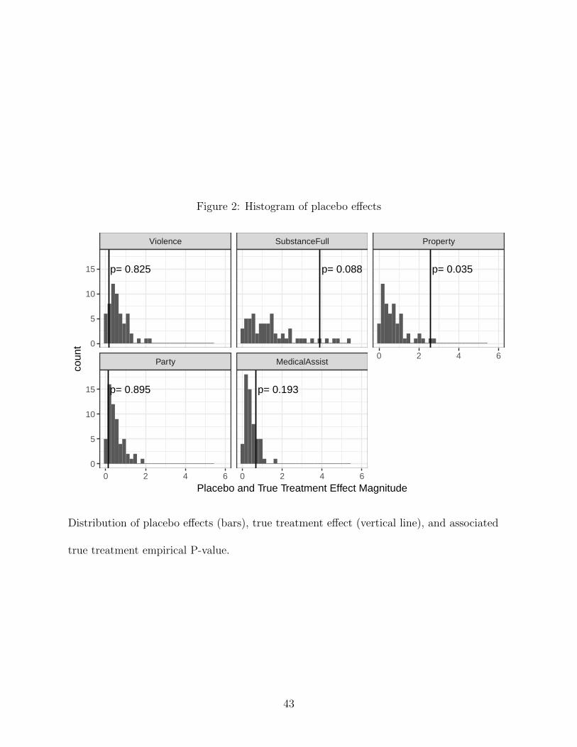
Figure 2: Histogram of placebo effects

p= 0.825

p= 0.895

p= 0.088

p= 0.193

p= 0.035

Party MedicalAssist

Violence SubstanceFull Property

0 2 4 6 0 2 4 6

0 2 4 60

5

10

15

0

5

10

15

Placebo and True Treatment Effect Magnitude

coun

t

Distribution of placebo effects (bars), true treatment effect (vertical line), and associated

true treatment empirical P-value.

43

Table 3: Marginal Effect of Additional $100 million PFD in First Week, 2000-2016

Violence Substance Property Party Medical

Assist

Marginal Effect -0.017 1.074** -0.347 -0.008 0.35***

(0.121) (0.422) (0.214) (0.103) (0.096)

P-value [0.888] [0.011] [0.104] [0.939] [0.000]

Bonferroni P-value [1.000] [0.044] [0.313] [1.000] [0.001]

Note: Newey-West Robust Errors in parentheses. Unadjusted p-values:

∗p<0.1; ∗∗p<0.05; ∗∗∗p<0.01

Deviation from average first week effect given a $100 million change in

distribution size. Estimated by Eq. 3. Violence includes: Homicide, as-

sault, and sexual assault. Substance category includes: incidents of driv-

ing while intoxicated, drunk and disorderly, drug possession, hit-and-runs,

and liquor law violations. Property crime includes burglary, robbery, theft,

and shoplifting. Party includes noise violation and loud/disruptive party

calls. Medical assistance calls only include police assistance of medical aid

for another department.

44

Table 5: Annualized & Monetized Changes from Cumulative 4-week Effect

Violence Substance Property Party Medical

Assist

Annual Incidents, 2016 5,128 11,971 12,744 2,741 7,962

4-weeks After PFD -16.31 125.6 -77.41 4.91 37.46

% Change After PFD -0.32% 1.05% -0.61% 0.18% 0.47%

95% Confidence [-0.83,0.20] [0.63,1.47] [-0.92,-0.29] [-0.52,0.88] [0.05,0.89]

Social Cost, $/Incident

Substance Property

Low Cost 35.92 4,305.06

High Cost 30,767.16 5,422.67

Total Social Cost, $1,000

Substance Property Net

Low Cost 4.51 -333.25 -328.74

High Cost 3,864.36 -419.77 3,444.59

Low social cost assumes the cost of crime comes only from its tangible components (i.e.

victim cost, criminal justice system costs, and crime career costs) and that alcohol abuse

does not induce any additional crime. High social cost assumes cost of crime is inclusive of

these factors, intangible cost (i.e. victim pain and suffering), and crime induced via alcohol

consumption. See Appendix B for details.

45