Embed Size (px)
Citation preview
Universal Banking, Asymmetric Information and the
Stock Market
Sanjay Banerji and Parantap Basu∗
February 2012, Preliminary, Comments welcome
ABSTRACT
The paper shows that attempts to sell stocks of borrowing firms by the universal banks
upon private information result in: (i) discounting of stock prices, (ii) a higher fraction of
ownership in the borrowing firm and a greater loan size, (iii) an increase in consumption
risk and precautionary savings of households. Hence, the size of the commercial banking
activity increases under asymmetric information at the expense of a higher consumption risk
borne by the households. The magnitude of the resulting risk premium is shown to be highly
sensitive to the probability of an aggregate negative shock perceived by the market.
∗Banerji: Finance Group, Nottingham University Business School, Nottingham University, Nottingham, NG81BB, [email protected]. Basu: Department of Economics and Finance, Durham Business School,Durham University, 23/26 Old Elvet, Durham DH1 3HY, UK (e-mail: [email protected]). Withoutimplicating, we acknowledge the constructive comments of an anonymous referee. The timely research assistanceof Congmin Peng, Zilong Wang, Sigit Wibowo and Shesadri Banerjee are gratefully acknowledged. The firstauthor gratefully acknowledges a seedcorn funding support from Durham Business School.
1

I. Introduction
A universal bank can sell insurance, hold equity in non financial firms and underwrite se-
curities in addition to its commercial banking activities. The hallmark of universal banking is
based on the premise that such a system could ensure household’s intertemporal consumption
smoothing when the bank undertakes depository acitivities while it could lead also to effi cient
risk sharing when it trades in securities. In recent times, such a financial institution has been
a subject of heated debate. Regulators in the UK and the USA are contemplating to curb
multifarious activities of these institutions, especially in areas where commercial banks enter
the business of underwriting equities.1 The current discussion partly mirrors the similar debate
that took place in mid 90’s prior to the repeal of Glass-Steagall Act.2
The aim of our paper is to demonstrate that the institution of universal banking works best in
the absence of any information friction. When the banker/underwriter holds private information
about the potential success or failure of the project in which the bank has an equity stake, it
gives rise to a typical lemon problem in the stock market because the rational financial market
already expects that banks could sell lemon securities in the wake of bad news. All stocks are
sold at a discount which means the emergence of a positive market premium whose magnitude
depends on the probability of a lemon. The macroeconomic effects of this information friction is
that consumption volatility increases. To mitigate this consumption risk, households undertakes
more saving. Banks make extra profit from selling lemon stocks which is channelled to greater
loan pushing. Thus commercial banking activity booms while aggregate investment and output
decline because of a higher risk adjusted market interest rate.
Our model provides a theoretical analysis of the effect of information asymmetry between
bankers/underwriters of stocks and shareholders on the aggregate stock market risk premium.
While there is an extensive literature that focuses on the quality of underwriting exclusively
related to investment banking side, hardly any effort is directed to analyze how such conflict of
1The Financial Times (11th April, 2011) wrote "Global banking regulation took a step towards convergenceafter the Independent Commission on Banking proposed measures that will bring the UK’s financial rules closerto the US. – The suggested changes are similar to regulations in the US, where banks are limited in the amountof deposits they can use for investment and commercial banking. The commission has recommended that largeuniversal banking groups in Britain, should ringfence their retail banking operations in the UK, safeguardingdepositors and essential payment services if other parts of the group run into trouble."
2See Benston (1990,1994), Barth et al. (2000), Krozner and Rajan (1994, 1997), Puri (1996), Gande et. al(1997) among many others who contributed to this lively debate.
2

interest impacts the aggregate stock market risk premium by altering the structure of financial
contracts.3Our results provide insights about the current debate on the financial crisis whether
the institution of universal banking in the USA via Gramm-Leach-Bliley Act of 1999 heightened
risk in the financial markets. In particular, questions arise whether some opportunistic banks
may dupe investors by selling "lemon securities" at an inflated price thus lowering the general
confidence.4
We analyze the effect of informational asymmetry on the stock market by introducing two
salient features in our simple two period model. First, we allow three kinds of shocks to hit
the economy: (i) an aggregate shock that motivates household’s precautionary savings decision,
(ii) an idiosyncratic project shocks that allows banks and household/borrower to effi ciently
share risks, (iii) a negative liquidity shock exclusively experienced by universal banks. Second
important feature of the model is a secondary stock market which opens before the resolution
of the idiosyncratic shock only when banks are subject to a liquidity shock. Once hit by such
a liquidity shock, banks may sell their claims to potential buyers in this secondary market.
The presence of a secondary share market combined with banks suffering liquidity shock paves
the way to accommodate conflict of interests between banks and share holders in the presence
information asymmetry. After receiving bad news about a project, a universal bank may sell
equities of the lemon borrowing firms to the uninformed household/shareholder with a pretense
that it has suffered a liquidity crunch. The demand for such speculative stock purchase comes
from the households who form an optimal portfolio of safe bank deposits and risky shares based
on risk-return trade-off.5
3We focus on traditional banks engaged in the process of transforming riskier loans to relatively safer deposits,which also hold equity in the borrowing firms as an outcome of optimal risk sharing mechanism. On the otherhand, the extant literature brings in either certification effects or economies of scope or transmission of informationto outsiders as the salient features of universal bankingFor example, see Kanatas and Qi (1998, 2003) for thetrade-off between economies of scope embedded within Universal banking versus deteriorations of quality ofprojects and innovations, Puri (1996, 1999) for the added role of certification of banks while underwriting debtsecurities versus conflicts of interests in equity holding, and Rajan (2002) for effi ciency of universal bankingrelated to competitiveness of the institutions. Our approach, on the other hand, is based on risk transformingrole of financial intermediation placed in the framework of optimal financial contracts where banks issue less riskydeposits to finance riskier loan by lending to large number of projects with uncorrelated risks. See, for example,Azariadis (1993, page 238-244), Bhattacharya and Thakor (1993) and Diamond (1984) and Gurley and Shaw(1960) for exposition of this view.
4The literature is divided about the effi cacy of universal banking system. See Benston (1994) for an excellentsurvey. Colvin (2007) analyzes two banking case studies for the Dutch system and alludes to the failure of theuniversal banking environment.
5Our paper is thus closer in spirit to the recent analysis of conflict of interest in other areas of financial servicesindustry rooted in the informational problems. See Mehran and Stultz (2007) (and other papers in the volume)for a comprehensive analysis of such conflicts pertinent to financial services industry originating from asymmetryof information.
3

Our simulation results show that in the presence of informational asymmetry, the stock
market premium is extremely sensitive to investor’s perception about the relative proportion of
lemons in the stock market. This anticipation is very much governed by the probability of a
negative aggregate shock to the economy. Even a minute increase in such a probability could
have a major effect on the stock market premium and the real interest rate. On the other hand,
changes in the probability of a liquidity crisis or project failure (which have idiosyncratic effects
on banks and individuals) have little effects on the stock market and the aggregate economy.
Although our paper shows the ineffi cient functioning of the financial markets under universal
banking in the presence of informational asymmetry, this does not necessarily imply that such
an arrangement should be replaced by non universal banking where banks are barred from
trading in securities. We show that non universal banking system fails to strike an effi cient
consumption risk sharing even under full information. The reason for this first order failure
of the non universal banking environment under full information is due to regulations which
prevent banks from sharing consumption risk by holding and trading securities in the wake of
a liquidity shock. The policy implication of our paper is that a universal banking could work
effi ciently if there is full disclosure of negative information and/or a tax on trading to discourage
sale of potential lemon sharesb y bank underwriters. This could lead to a near full risk sharing
in consumption except for cases of aggregate risk.
The paper is organized as follows. The following section lays out the model and the envi-
ronment. Section 3 solves a baseline model of universal banking with full information about
the states of nature. Section 4 introduces the asymmetric information about the states and the
consequent conflict of interest between banks and the stockholders. Section 5 reports the results
from a simulation experiment based on our model. Section 6 concludes.
II. The Model
A. Households
We consider a simple intertemporal general equilibrium model in which there is a continuum
of identical agents in the unit interval who live only for two periods. At t = 1, a stand-in
agent is endowed with y units of consumption goods, and she also owns a project requiring a
physical investment of k units of capital in the current period which produces a random cash
flow/output in the next period. The production of output is subject to two types of binary
4
shocks: (i) an aggregate shock, (ii) an idiosyncratic shock. The aggregate shock is transmitted
to intermediaries/agents via a probabilistic signal. A signal conveys news about the state which
could be high (h) and low (l) with probabilities σh and 1 − σh respectively. A low signal (a
recessionary state) triggers widespread liquidation of the current projects and the project is
liquidated at a near zero continuation value (m).6 If the signal is h, agents are still subject to
idiosyncratic shock which manifests in terms of a project success with probability p and failure
with probability 1− p.7
To sum up, the random output in next period has the following representation:
m with probability 1− σh
θgg(k) with probability σhp
θbg(k) with probability σh(1− p)
where θg > θb
B. Banks
Competitive universal banks offer a contract that stipulates (a) deposits (s) , (b) loans (f), and
(c) contingent payments (di, i = g, b). After writing such a contract and before the realization
of the random shock, banks may experience a liquidity shock (C) which necessitates banks to
sell their ownerships claims (θig(k)− di) to the public in a secondary market at a price q.8 Let
n be the number of such securities. Let x and nx denote the states of liquidity shock and no
such shock with probabilities γ and 1−γ.This interim period when the secondary market opens
6This assumption is made in order to preserve a simple structure for analysis. Instead of assuming a fixedsalvage value, we could have alternatively proceeded with a lower probability of success in individual projects inthe event of a low aggregative signal and this would not change our results.
7Since this type of risk is distributed independently across infinite number of projects, the law of large numberholds in an economy populated by continuum of agents so that p fraction of individuals is more successful thanthe rest. On the other hand, no such law holds for a low aggregate state.
8We only allow the banks to have a liquidity shock and exclude individuals to have similar problem because itmakes the exposition simpler and also owing to the fact that the primary purpose of the paper is to investigate theconsequence of banks’holding of tradable financial assets on the rest of the economy under both full informationand asymmetric information. In particular, we show later how the private information gathered by banks regardingthe aggregate state has both financial and real effects. In this scenario, allowing individuals to incur liquidityproblems will add further noise in the financial market and will actually strengthen our results.
5
is dated as 1.5.9
At this interim date 1.5, the bank may also acquire an early signal about the aggregate shock.
If the signal is high (h) with probability σh, the project’s value upon continuation is greater
than the same under liquidation. If the signal is low, it means that banks get early information
that most of the projects will turn out to be a lemon with negligible value (close to zero m).10
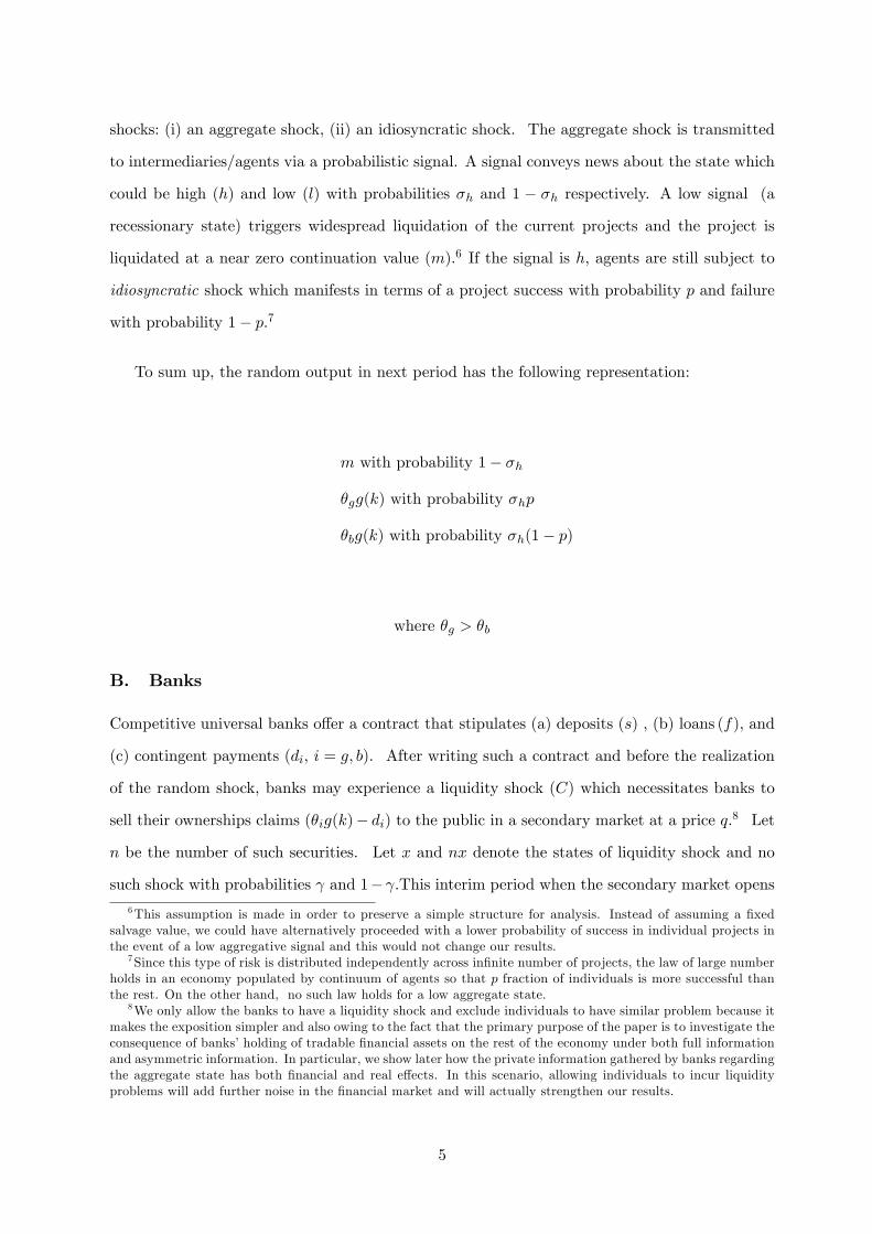
At t = 2, uncertainties get resolved and all agents receive pay-off according to the contracts
written at date t = 0, which, in turn, depends on (a) resolution of individual uncertainty and
(b) occurrences of liquidity shocks of banks . The Figure 1 summarizes the time-line in terms
of a flow chart.
Figure 1 : Timeline for Universal Banking
A few comments are in order to justify the existence of multiple shocks in the model. The
presence of idiosyncratic shocks to individual projects induce banks and individuals to allocate
risk optimally among themselves. Banks divide ownership claims in the borrowing firms between
themselves and the household/share holders which is a typical feature of universal banking. This
division of ownership serves as a mechanism for risk sharing with the households. Second, the
9Under universal banking, banks or intermediaries can hold securities which are otherwise unrestricted andtradable compared with the system where banks can only hold debt securities which cannot easily be traded inthe financial/debt market.10The rationale behind such assumption is that since banks lend and monitor a large number of projects across
the economy, they gather expertise to collect information relevant not only to a single project but can extractinformation about the overall economy better than the households. This is a standard function of banks whoare also known as ”informed lenders”(see Freixas and Rochet, 2008). However, the main difference between theuniversal and non universal banking is that the former can take its informational advantage by selling stocks toothers before the bad event realizes while the latter cannot do such things because they are not allowed to holdequity in the borrowing firms.
6
introduction of liquidity shock by banks directly provides rationale for banks selling stocks to
investors in the secondary market at date 1.5 when the bank could receive bad news about the
project and sell such lemon stocks with a pretense of a liquidity shock. Finally, the aggregate
shock also gives the rationale for households to hold claims in the form of bank deposits (i.e., its
demand for deposits in addition to holding financial claims via optimal contracts). Household’s
saving also provides liquidity to the stock market when it opens at the intermediate date 1.5.
Saving thus performs two roles: (i) consumption smoothing, (ii) liquidity for speculative purchase
of shares.
The expected profit of the bank is thus:
πbank = σhγ.[p{θgg(k)− dg}
+(1− p).{θbg(k)− db}] + σh(1− γ).(qn− C)
+(1− σh)m− f.(1 + rσh)
(1)
We just note that the loan servicing cost is rσh because banks do not pay any interest on
savings in a low signal state which occurs with probability 1 − σh. Hereafter, we assume that
banks issue just enough shares to cover the liquidity crunch which means n = C/q.
C. Preferences
The utility function of each household/ borrower/depositor is additively separable in consump-
tion at each date and is of the form:
U = u(c1) + v(c2) (2)
where c1= consumption in period i, i = 1, 2, u(·) and v(·) are: (a) three times continuously
differentiable, (b) concave, and (c) have a convex marginal utility function. Hence, agents are
risk-averse and in addition have a precautionary motive for savings.
Apart from the current period, in period 2 there are 5 possible states and the expected utility
7
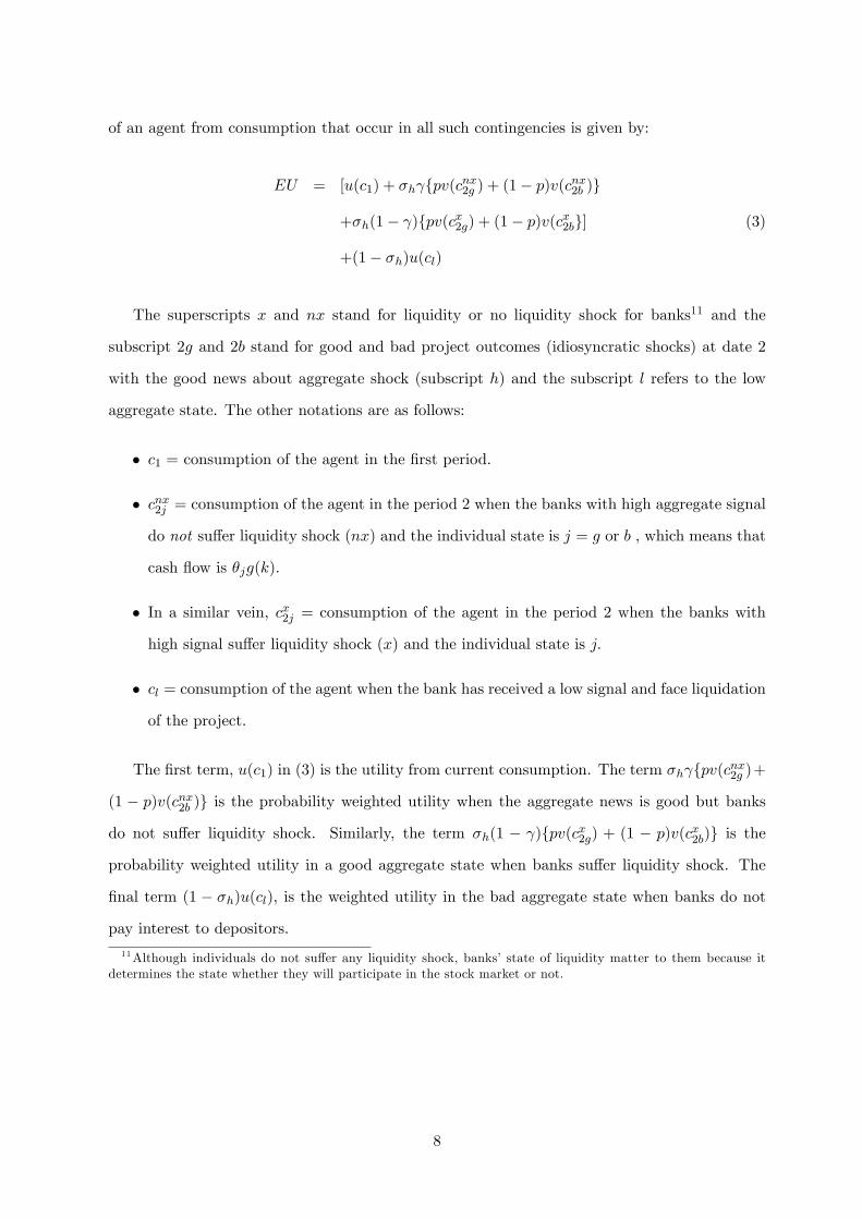
of an agent from consumption that occur in all such contingencies is given by:
EU = [u(c1) + σhγ{pv(cnx2g ) + (1− p)v(cnx2b )}
+σh(1− γ){pv(cx2g) + (1− p)v(cx2b}] (3)
+(1− σh)u(cl)
The superscripts x and nx stand for liquidity or no liquidity shock for banks11 and the
subscript 2g and 2b stand for good and bad project outcomes (idiosyncratic shocks) at date 2
with the good news about aggregate shock (subscript h) and the subscript l refers to the low
aggregate state. The other notations are as follows:
• c1 = consumption of the agent in the first period.
• cnx2j = consumption of the agent in the period 2 when the banks with high aggregate signal
do not suffer liquidity shock (nx) and the individual state is j = g or b , which means that
cash flow is θjg(k).
• In a similar vein, cx2j = consumption of the agent in the period 2 when the banks with
high signal suffer liquidity shock (x) and the individual state is j.
• cl = consumption of the agent when the bank has received a low signal and face liquidation
of the project.
The first term, u(c1) in (3) is the utility from current consumption. The term σhγ{pv(cnx2g )+
(1 − p)v(cnx2b )} is the probability weighted utility when the aggregate news is good but banks
do not suffer liquidity shock. Similarly, the term σh(1 − γ){pv(cx2g) + (1 − p)v(cx2b)} is the
probability weighted utility in a good aggregate state when banks suffer liquidity shock. The
final term (1 − σh)u(cl), is the weighted utility in the bad aggregate state when banks do not
pay interest to depositors.
11Although individuals do not suffer any liquidity shock, banks’ state of liquidity matter to them because itdetermines the state whether they will participate in the stock market or not.
8
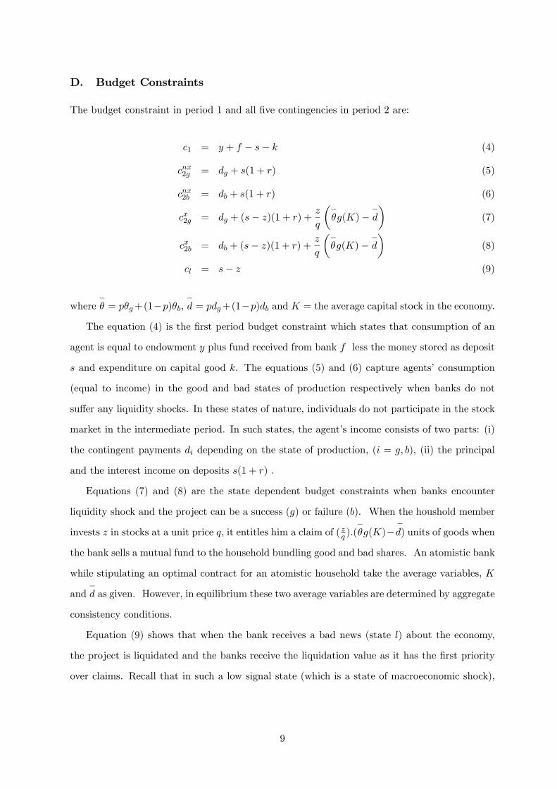
D. Budget Constraints
The budget constraint in period 1 and all five contingencies in period 2 are:
c1 = y + f − s− k (4)
cnx2g = dg + s(1 + r) (5)
cnx2b = db + s(1 + r) (6)
cx2g = dg + (s− z)(1 + r) +z
q
(−θg(K)−
−d
)(7)
cx2b = db + (s− z)(1 + r) +z
q
(−θg(K)−
−d
)(8)
cl = s− z (9)
where−θ = pθg+(1−p)θb,
−d = pdg+(1−p)db and K = the average capital stock in the economy.
The equation (4) is the first period budget constraint which states that consumption of an
agent is equal to endowment y plus fund received from bank f less the money stored as deposit
s and expenditure on capital good k. The equations (5) and (6) capture agents’consumption
(equal to income) in the good and bad states of production respectively when banks do not
suffer any liquidity shocks. In these states of nature, individuals do not participate in the stock
market in the intermediate period. In such states, the agent’s income consists of two parts: (i)
the contingent payments di depending on the state of production, (i = g, b), (ii) the principal
and the interest income on deposits s(1 + r) .
Equations (7) and (8) are the state dependent budget constraints when banks encounter
liquidity shock and the project can be a success (g) or failure (b). When the houshold member
invests z in stocks at a unit price q, it entitles him a claim of ( zq ).(−θg(K)−
−d) units of goods when
the bank sells a mutual fund to the household bundling good and bad shares. An atomistic bank
while stipulating an optimal contract for an atomistic household take the average variables, K
and−d as given. However, in equilibrium these two average variables are determined by aggregate
consistency conditions.
Equation (9) shows that when the bank receives a bad news (state l) about the economy,
the project is liquidated and the banks receive the liquidation value as it has the first priority
over claims. Recall that in such a low signal state (which is a state of macroeconomic shock),
9

banks are unable to make full payment and only return the deposits s to the households.12
III. Universal Banking under Full Information
As a baseline case, we first lay out the equilibrium contract in a full information scenario.
For a given interest rate r and stock price q, each bank offers a package to the household which
includes (i) the loan size f , (ii) payments to the same household di contingent on realizations
of idiosyncratic states. In return, the household must put in a deposit s at the same bank and
undertake a physical investment k in the project.13
Such a package is stipulated by the bank that solves the expected utility of the household
subject to the condition that these universal banks offering such competitive contracts satisfy
the participation constraint which means that they must break even.
Hence, the optimization problem is to maximize the expected utility (3) subject to the budget
constraints given by (4) through (9) and zero profit constraint of the intermediary, i.e.
πbank = σhγ [p{θgg(k)− dg}+ (1− p){θbg(k)− db}]+(1−σh)m+σh(1−γ)(qn−C)−f.(1+rσh) ≥ 0
Since there is full information, the agent exactly knows the node at which the bank operates.
Thus at a low signal state agents know that a stock market will not open at date 1.5. This
immediately means that z = 0 at this low signal state.
A. Interest rate
We assume here that the real interest rate, r is fixed by a policy rule. Any discrepancy between
borrowing f and lending s is financed by a net inflow of foreign funds (call it NFI) from
abroad at this targeted interest rate.14The appendix provides the details of the market clearing
conditions.
Proposition 1: The competitive equilibrium contract has the following properties:
(i) Contingent Payments: dg = db = d (say) such that γu′(c1)1+rσh
= v′(d+ s(1 + r))
12Nothing fundamentally changes in our model if we assume instead that banks return only a fraction of savingsin a low aggregate state.13The contingent claims di are not traded in a market. These are stipulated by optimal contracts and that is
why there is no price attached to each such contingent claim.14This is a simplifying assumption that rules out the second order effect of the financial operations of banks
and households on the real interest rate. This simplification is made to understand the behaviour of householdsaving and bank loans in the presence of information friction. In the next section where we undertake simulation,we allow the interest rate to vary to equilibrate the loan market.
10

(ii) Share Price: q = EX̃1+r where EX̃ =
−θg(K)−
−d.
(iii) Consumption: cnx2g = cnx2b = cx2g = cx2b = d+ s(1 + r) > cl = s
(iv) Saving: u′(c1) =[(1−σh)(1+rσh)1−γσh+rσh(1−γ)
]v′(s)
(v) Investment: γ−θ g′(k) = σ−1h + r where
−θ = pθg + (1− p)θb and
(vi) Loan: f = σhγ(−θg(k)−d)+(1−σh)m+σh(1−γ)(qn−C)
1+rσh
(vii) Consistency of Expectations: k = K
Proof : Appendix A.
Discussion: (i), (iv), (v) and (vi) together determine {d, s,K, f } and the equation (ii)
determines q, given an exogenous r. Stocks have fair market value as seen in (ii) and the
risk premium is thus zero. The risk neutral bank bears the whole idiosyncratic risks which
explains why the market risk premium is zero. (i) and (ii) together state that conditional on
the realization of high signal, an agent receives a constant sum d across all states of nature.
Although idiosyncratic risk is washed out in the high state h, in the low state individuals are
still exposed to negative aggregate shock which explains the last inequality of (iii). The holding
of deposit in the form of savings acts as an instrument to deal with this situation. If there is no
aggregate risk, σh = 1, optimal saving is zero as seen from (iv) which highlights the precautionary
motive for savings. (v) states that the expected marginal productivity of investment equals the
risk adjusted interest rate, σ−1h + r . The physical investment K is lower if the probability of
low aggregate state is higher (lower σh). (vi) states the equilibrium loan size obtained from
bank’s zero profit condition. Finally, (vii) states the aggregate consistency condition that sum
of all individual capital capital stocks equals the aggregate capital and over a unit interval.
The results in the proposition 1 serve to capture the basic functioning of the universal
banking in the simplest possible full information framework. The universal banks optimally
share project risks by offering a riskfree payment d and the residual θjg(k) − d is kept by the
bank.15 Without any conflicts of interest (asymmetric information), this is a Pareto optimal
contract. It eliminates idiosyncratic uncertainties in household consumption and makes stock
price trade at a fair market value.16
15This contract is equivalent to: (i) agents holding a preferred stock (or any other instrument that ensures aconstant sum in all contingencies within good aggregate state), and (ii) banks owning ordinary stocks and thusbear all the residual risks. Thus, banks holding of equity, a hallmark of universal banking, emerges as a mechanismof an optimum allocation of risk.16Although banks are holding the residual claim in each state but our conclusions are not sensitive to this
11

IV. Universal Banking under Asymmetric Information
Using the baseline model of full information described in the preceding section, we now turn
to the case of asymmetric information. The basic tenet of such informational asymmetry is that
banks hold private information about the realization of the aggregate business cycle as well the
liquidity shocks.17 In other words, banks observe true realizations of both liquidity shocks and
the realization of the signal regarding the macro business cycle state but agents know only the
distribution of liquidity shocks and the signals. Since interest payment on deposits take place at
t = 2 after the transaction in intermediate stock market, if the stock market opens at date 1.5,
agents cannot ascertain whether banks have received a low signal or simply suffered a liquidity
shock. This gives rise to a typical lemon problem because universal banks with a low realization
of the signal may sell off the equity held by them in the borrowing firm with a pretense of the
liquidity shock. This problem of selling lemon stocks can emerge only in the universal banking
system as opposed to the non universal system where banks are barred to hold equity in the
borrowing firms.
Think of the agent situated at the node t = 1.5. At this node, she only observes whether
the stock market has opened or not. If the stock market does not open then she knows for sure
(a) high signal has occurred and (b) no bank has suffered a liquidity shock. Of course, she could
still either succeed or fail. Given that (a) and (b) happen with probability σhγ, the expected
utility (up to this node) is:
σhγ[pv(dg + s(1 + r)) + (1− p)v(db + s(1 + r))].
Now if the equity market opens at the intermediate date 1.5 where a financial intermediary
sells stocks, an agent concludes that either the bank has received a low signal (with a probability
of 1−σh) ) or the bank has received good news about the aggregate shock but it is still selling the
stock because it has suffered a liquidity shock. The probability of the latter event is σh(1− γ).
result. In an earlier version of the paper, we had introduced borrowers’moral hazard which leads banks to holdcontingent claims that vary across good and bad states. We dropped the issue of borrowers’moral hazard in thisversion because it does not add new insights and our main results are also unchanged with this modification.17The banks can observe the aggregate shock at least in a partial manner because they lend it to agents
economy-wide and collect/collate information from each borrower. Hence, they tend to have economy-wideinformation while each agent is too small to acquire aggregate signal. However, bank’s signal about aggregateand idiosyncratic shocks need not be perfect and could be even noisy. For the sake of parsimony, simplicity, andwithout compromising our results below, we ignore the noisiness of bank’s signal about aggregate shock and theirprivate information about individual projects.
12

Hence, an individual at the node at date 1.5 when she is observing someone selling the stocks
will compute the probability(
σh(1−γ)σh(1−γ)+(1−σh) = σh(1−γ)
(1−γσh)
)that the stock is not a lemon.
The optimal contract problem can be thus written as:
max{dg ,db,s,z,l,k}
EU = [u(y + f − s− k)] + σhγ[pv(dg + s(1 + r)) + (1− p)v(db + s(1 + r))]
+(1− γσh) ·((σh(1−γ)(1−γσh)
))[pv(dg + (s− z)(1 + r) zqEX̃)
+(1− p)v(db + (s− z)(1 + r) + zqEX̃)]
+(1− γσh)((1−σh)(1−γσh)
)v(s− z)
subject to
πbank = σhγ [p{θgg(k)− dg}+ (1− p){θbg(k)− db}]+σh(1−γ)(qn−C)+(1−σh)(qn+m)−f(1+rσh) ≥ 0
(10)
There are two important features of this optimal contract problem which require clarification.
First, while writing a contract with the bank, household/shareholder takes into account that
banks can sell off stocks in the midway (at date 1.5) upon bad news and thus they may incur
capital losses. Second, the zero profit constraint (10) now contains an additional term (1−σh)qn
which is the extra expected income of the banks from selling securities upon bad news.
Proposition 2: The equilibrium contract under asymmetric information has the following
properties:
(ia) Contingent Payments: dga = dba = da (say) andγu′(c1)1+rσh
= γv′(cnx2a ) + (1− γ)v′(cx2a)
(iia) Share Price: EX̃aq − (1 + r) =
v′{(sa−z)}
v′{da+(sa−z)(1+r)+ z
qE˜X
} 1−σh
σh(1−γ) > 0 where EX̃a
=
(−θg(K)−
−da
n
)(iiia) Consumption: cx2g = cx2b ≡ cx2a = da+sa(1+r)+
{EX̃aq − (1 + r)
}·z > cnx2g = cnx2b = cnx2a
= da + sa(1 + r) > cla = sa − z
(iva) Saving: u′(c1a) =[(1−σh)(1+rσh)1−γσh+rσh(1−γ)
]v′(sa − z)
(va) Investment: γ−θg′(k) = σ−1h + r where
−θ = pθh + (1− p)θl and
(via) Loan: fa = σhγ(−θg(k)−
−da)+(1−σh)qn+σh(1−γ)(qn−C)
1+rσh
(viia) Consistency of Expectations: k = K
13
Proof : Appendix B.
Discussions: We denote the subscript a as the solution of the variables under asymmetric
information. (ia) shares the same feature as (i). Idiosyncratic risks are again borne by the risk
neutral bank and household receives a riskfree payment da for its ownership claim to the project.
The major difference from the baseline full information setting appears in (iia). Since banks
can potentially sell lemon securities in the midway at date 1.5, the optimal contract embeds
this possibility. (iia) shows that stocks sell at a discount in the sense that the price is less than
the discounted value of the cash flow. To put it alternatively, a positive market risk premium
emerges in equilibrium to reflect this lemon problem.
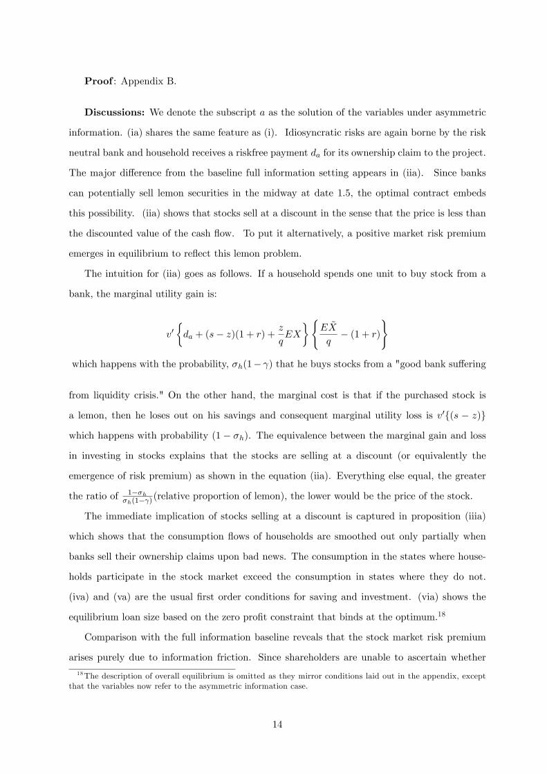
The intuition for (iia) goes as follows. If a household spends one unit to buy stock from a
bank, the marginal utility gain is:
v′{da + (s− z)(1 + r) +
z
qEX
}{EX̃
q− (1 + r)
}
which happens with the probability, σh(1− γ) that he buys stocks from a "good bank suffering
from liquidity crisis." On the other hand, the marginal cost is that if the purchased stock is
a lemon, then he loses out on his savings and consequent marginal utility loss is v′{(s − z)}
which happens with probability (1 − σh). The equivalence between the marginal gain and loss
in investing in stocks explains that the stocks are selling at a discount (or equivalently the
emergence of risk premium) as shown in the equation (iia). Everything else equal, the greater
the ratio of 1−σhσh(1−γ)(relative proportion of lemon), the lower would be the price of the stock.
The immediate implication of stocks selling at a discount is captured in proposition (iiia)
which shows that the consumption flows of households are smoothed out only partially when
banks sell their ownership claims upon bad news. The consumption in the states where house-
holds participate in the stock market exceed the consumption in states where they do not.
(iva) and (va) are the usual first order conditions for saving and investment. (via) shows the
equilibrium loan size based on the zero profit constraint that binds at the optimum.18
Comparison with the full information baseline reveals that the stock market risk premium
arises purely due to information friction. Since shareholders are unable to ascertain whether
18The description of overall equilibrium is omitted as they mirror conditions laid out in the appendix, exceptthat the variables now refer to the asymmetric information case.
14
banks sell off shares due to liquidity shock or arrival of bad news, additional premium is required
to lure households to buy shares. The emergence of a risk premium (or stocks selling at a
discount) prevents the agents from smoothing out consumption across nx and x states. In sharp
contrast, a full insurance across nx and x is possible under full information setting because
agents are perfectly informed about the nodes at which banks sell stocks.
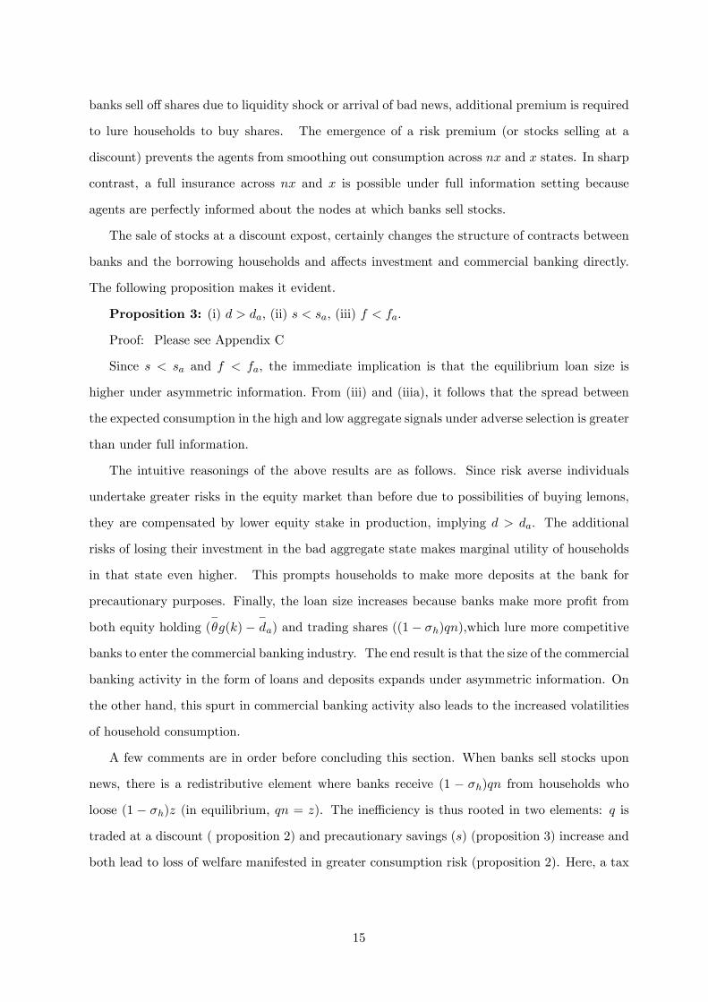
The sale of stocks at a discount expost, certainly changes the structure of contracts between
banks and the borrowing households and affects investment and commercial banking directly.
The following proposition makes it evident.
Proposition 3: (i) d > da, (ii) s < sa, (iii) f < fa.
Proof: Please see Appendix C
Since s < sa and f < fa, the immediate implication is that the equilibrium loan size is
higher under asymmetric information. From (iii) and (iiia), it follows that the spread between
the expected consumption in the high and low aggregate signals under adverse selection is greater
than under full information.
The intuitive reasonings of the above results are as follows. Since risk averse individuals
undertake greater risks in the equity market than before due to possibilities of buying lemons,
they are compensated by lower equity stake in production, implying d > da. The additional
risks of losing their investment in the bad aggregate state makes marginal utility of households
in that state even higher. This prompts households to make more deposits at the bank for
precautionary purposes. Finally, the loan size increases because banks make more profit from
both equity holding (−θg(k)−
−da) and trading shares ((1− σh)qn),which lure more competitive
banks to enter the commercial banking industry. The end result is that the size of the commercial
banking activity in the form of loans and deposits expands under asymmetric information. On
the other hand, this spurt in commercial banking activity also leads to the increased volatilities
of household consumption.
A few comments are in order before concluding this section. When banks sell stocks upon
news, there is a redistributive element where banks receive (1 − σh)qn from households who
loose (1 − σh)z (in equilibrium, qn = z). The ineffi ciency is thus rooted in two elements: q is
traded at a discount ( proposition 2) and precautionary savings (s) (proposition 3) increase and
both lead to loss of welfare manifested in greater consumption risk (proposition 2). Here, a tax
15

on trading can partially ameliorate this welfare loss.19
The results in proposition 3 are established in the neighbourhood of full information equi-
librium. In the next section, we perform a sensitivity analysis with the aid of a simulation
experiment to check the robustness of these results.
V. An Illustrative Simulation
There are three levels of risk in our model: (i) an aggregate business cycle risk (σh) facing
all agents, (ii) an aggregate liquidity risk γ facing all banks, and (iii) idiosyncratic project risk p
facing only the household entrepreneurs. The aim of this section is to ascertain the quantitative
effects of these three risks on the stock market and the economy based on our stylized model. We
assume logarithmic utility functions which mean u(c1) = ln c1 and v(c2) = ln c2. The production
function is assumed to be Cobb-Douglas, meaning g(k) = kα with 0 < α < 1.
There are nine parameters in this stylized model, namely y, σh, γ, p, α, θh, θl, C and m. The
first period output y is normalized at unity with a view to to express relevant macroeconomic
aggregates such as consumption c1, saving s, and other relevant macroeconomic variables as
a percent of the first period output (GDP). The average growth rate of the economy is then
σh−θkα + (1− σh)m, which can then be compared to the long run average growth rate of GDP.
After fixing the capital share parameter α at its conventional value 0.36 and normalizing the
low state total factor productivity (TFP) parameter, θl at unity, the high state TFP, θh is fixed
to target a 3.5% long run average annual growth rate of GDP in the US during the same sample
period 1960-2006.20
Among the three probability parameters, σh, γ, p , the probability of the high aggregate
shock, σh is critical in determining the stock market discount. To see this clearly, set σh
equal to unity which eliminates aggregate business cycle risk. It is straightforward to verify
from (iv) of proposition 1 that saving, s is zero because in a riskfree aggregate state there
is zero precautionary demand for saving. The stock market discount is also zero which can
be easily verified from (iia) in proposition 2 by plugging a logarithmic utility specification.
We fix σh to target a baseline 7% annual stock market discount based on the estimate of
19Though one has to note the deadweight losses due to taxes and the fact that it also penalizes the honestbanks who sell upon liquidity. But a small tax can be welfare improving.20 In the context of our two period steady state model, the ratio of the second period to first period outputs
approximates the long run average GDP growth rate.
16
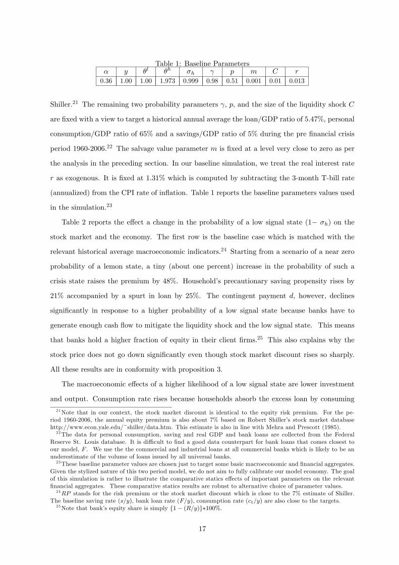
Table 1: Baseline Parametersα y θl θh σh γ p m C r
0.36 1.00 1.00 1.973 0.999 0.98 0.51 0.001 0.01 0.013
Shiller.21 The remaining two probability parameters γ, p, and the size of the liquidity shock C
are fixed with a view to target a historical annual average the loan/GDP ratio of 5.47%, personal
consumption/GDP ratio of 65% and a savings/GDP ratio of 5% during the pre financial crisis
period 1960-2006.22 The salvage value parameter m is fixed at a level very close to zero as per
the analysis in the preceding section. In our baseline simulation, we treat the real interest rate
r as exogenous. It is fixed at 1.31% which is computed by subtracting the 3-month T-bill rate
(annualized) from the CPI rate of inflation. Table 1 reports the baseline parameters values used
in the simulation.23
Table 2 reports the effect a change in the probability of a low signal state (1− σh) on the
stock market and the economy. The first row is the baseline case which is matched with the
relevant historical average macroeconomic indicators.24 Starting from a scenario of a near zero
probability of a lemon state, a tiny (about one percent) increase in the probability of such a
crisis state raises the premium by 48%. Household’s precautionary saving propensity rises by
21% accompanied by a spurt in loan by 25%. The contingent payment d, however, declines
significantly in response to a higher probability of a low signal state because banks have to
generate enough cash flow to mitigate the liquidity shock and the low signal state. This means
that banks hold a higher fraction of equity in their client firms.25 This also explains why the
stock price does not go down significantly even though stock market discount rises so sharply.
All these results are in conformity with proposition 3.
The macroeconomic effects of a higher likelihood of a low signal state are lower investment
and output. Consumption rate rises because households absorb the excess loan by consuming
21Note that in our context, the stock market discount is identical to the equity risk premium. For the pe-riod 1960-2006, the annual equity premium is also about 7% based on Robert Shiller’s stock market databasehttp://www.econ.yale.edu/~shiller/data.htm. This estimate is also in line with Mehra and Prescott (1985).22The data for personal consumption, saving and real GDP and bank loans are collected from the Federal
Reserve St. Louis database. It is diffi cult to find a good data counterpart for bank loans that comes closest toour model, F . We use the the commercial and industrial loans at all commercial banks which is likely to be anunderestimate of the volume of loans issued by all universal banks.23These baseline parameter values are chosen just to target some basic macroeconomic and financial aggregates.
Given the stylized nature of this two period model, we do not aim to fully calibrate our model economy. The goalof this simulation is rather to illustrate the comparative statics effects of important parameters on the relevantfinancial aggregates. These comparative statics results are robust to alternative choice of parameter values.24RP stands for the risk premium or the stock market discount which is close to the 7% estimate of Shiller.
The baseline saving rate (s/y), bank loan rate (F/y), consumption rate (c1/y) are also close to the targets.25Note that bank’s equity share is simply {1− (R/y)}∗100%.
17
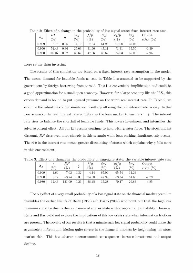
Table 2: Effect of a change in the probability of low signal state: fixed interest rate case
σhRP(%)
qs/y(%)
f/y(%)
d/y(%)
c1/y(%)
k/y(%)
Outputeffect (%)
0.999 6.76 0.36 4.19 7.34 64.28 67.08 36.05 -0.990 54.43 0.36 25.03 31.90 47.11 71.31 35.55 -1.390.980 109.07 0.32 38.62 47.66 35.62 74.03 35.00 -2.95
more rather than investing.
The results of this simulation are based on a fixed interest rate assumption in the model.
The excess demand for loanable funds as seen in Table 1 is assumed to be supported by the
government by foreign borrowing from abroad. This is a convenient simplification and could be
a good approximation for a small open economy. However, for a large economy like the U.S., this
excess demand is bound to put upward pressure on the world real interest rate. In Table 2, we
examine the robustness of our simulation results by allowing the real interest rate to vary. In this
new scenario, the real interest rate equilibrates the loan market to ensure s = f . The interest
rate rises to balance the shortfall of loanable funds. This lowers investment and intensifies the
adverse output effect. All our key results continue to hold with greater force. The stock market
discount, RP rises even more sharply in this scenario while loan pushing simultaneously occurs.
The rise in the interest rate means greater discounting of stocks which explains why q falls more
in this environment.
Table 3: Effect of a change in the probability of aggregate state: the variable interest rate case
σhr
(%)RP(%)
qf/y(%)
d/y(%)
c1/y(%)
k/y(%)
Outputeffect (%)
0.999 4.69 7.02 0.32 4.14 65.09 65.74 34.23 -0.990 9.12 58.74 0.30 24.58 47.99 68.34 31.66 -2.790.980 12.43 121.09 0.26 38.45 35.28 70.17 29.83 -4.85
The big effect of a very small probability of a low signal state on the financial market premium
resembles the earlier results of Reitz (1988) and Barro (2009) who point out that the high risk
premium could be due to the occurrence of a crisis state with a very small probability. However,
Reitz and Barro did not explore the implications of this low crisis state when information frictions
are present. The novelty of our results is that a minute such low signal probability could make the
asymmetric information friction quite severe in the financial markets by heightening the stock
market risk. This has adverse macroeconomic consequences because investment and output
decline.
18
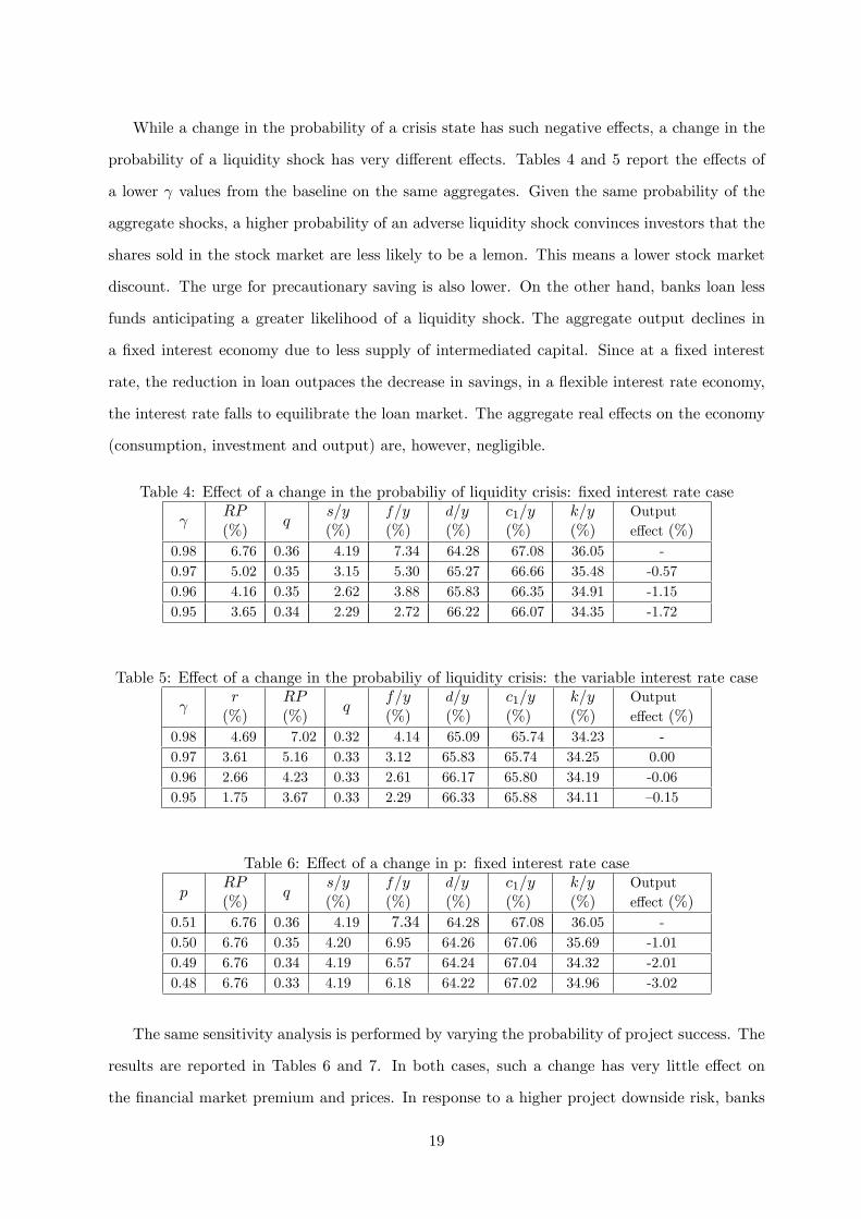
While a change in the probability of a crisis state has such negative effects, a change in the
probability of a liquidity shock has very different effects. Tables 4 and 5 report the effects of
a lower γ values from the baseline on the same aggregates. Given the same probability of the
aggregate shocks, a higher probability of an adverse liquidity shock convinces investors that the
shares sold in the stock market are less likely to be a lemon. This means a lower stock market
discount. The urge for precautionary saving is also lower. On the other hand, banks loan less
funds anticipating a greater likelihood of a liquidity shock. The aggregate output declines in
a fixed interest economy due to less supply of intermediated capital. Since at a fixed interest
rate, the reduction in loan outpaces the decrease in savings, in a flexible interest rate economy,
the interest rate falls to equilibrate the loan market. The aggregate real effects on the economy
(consumption, investment and output) are, however, negligible.
Table 4: Effect of a change in the probabiliy of liquidity crisis: fixed interest rate case
γRP(%)
qs/y(%)
f/y(%)
d/y(%)
c1/y(%)
k/y(%)
Outputeffect (%)
0.98 6.76 0.36 4.19 7.34 64.28 67.08 36.05 -0.97 5.02 0.35 3.15 5.30 65.27 66.66 35.48 -0.570.96 4.16 0.35 2.62 3.88 65.83 66.35 34.91 -1.150.95 3.65 0.34 2.29 2.72 66.22 66.07 34.35 -1.72
Table 5: Effect of a change in the probabiliy of liquidity crisis: the variable interest rate case
γr
(%)RP(%)
qf/y(%)
d/y(%)
c1/y(%)
k/y(%)
Outputeffect (%)
0.98 4.69 7.02 0.32 4.14 65.09 65.74 34.23 -0.97 3.61 5.16 0.33 3.12 65.83 65.74 34.25 0.000.96 2.66 4.23 0.33 2.61 66.17 65.80 34.19 -0.060.95 1.75 3.67 0.33 2.29 66.33 65.88 34.11 —0.15
Table 6: Effect of a change in p: fixed interest rate case
pRP(%)
qs/y(%)
f/y(%)
d/y(%)
c1/y(%)
k/y(%)
Outputeffect (%)
0.51 6.76 0.36 4.19 7.34 64.28 67.08 36.05 -0.50 6.76 0.35 4.20 6.95 64.26 67.06 35.69 -1.010.49 6.76 0.34 4.19 6.57 64.24 67.04 34.32 -2.010.48 6.76 0.33 4.19 6.18 64.22 67.02 34.96 -3.02
The same sensitivity analysis is performed by varying the probability of project success. The
results are reported in Tables 6 and 7. In both cases, such a change has very little effect on
the financial market premium and prices. In response to a higher project downside risk, banks
19
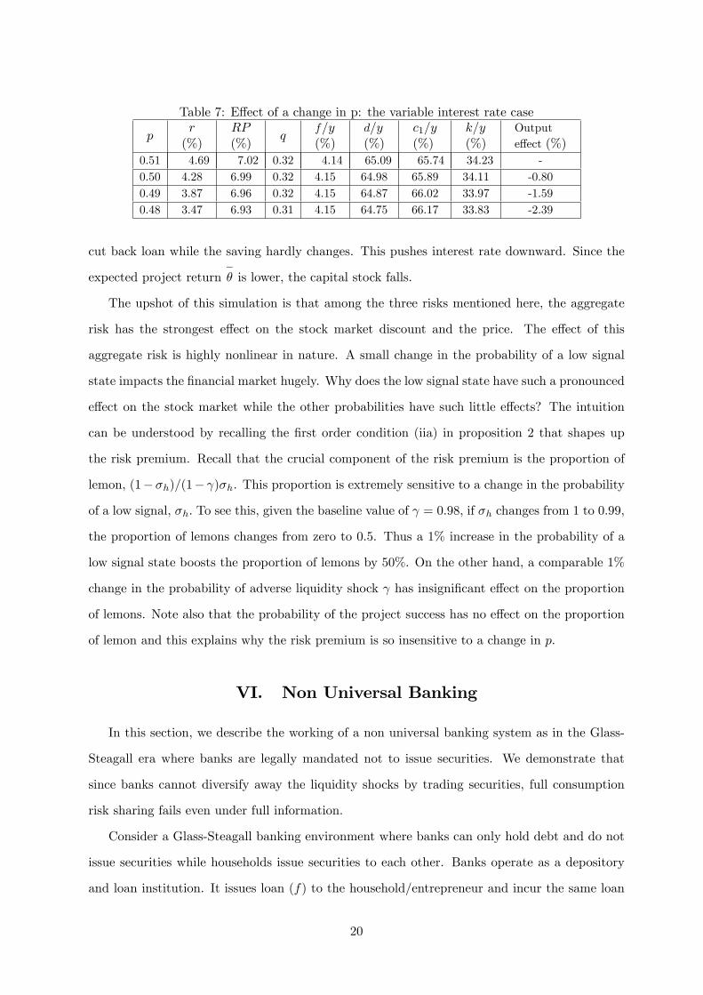
Table 7: Effect of a change in p: the variable interest rate case
pr
(%)RP(%)
qf/y(%)
d/y(%)
c1/y(%)
k/y(%)
Outputeffect (%)
0.51 4.69 7.02 0.32 4.14 65.09 65.74 34.23 -0.50 4.28 6.99 0.32 4.15 64.98 65.89 34.11 -0.800.49 3.87 6.96 0.32 4.15 64.87 66.02 33.97 -1.590.48 3.47 6.93 0.31 4.15 64.75 66.17 33.83 -2.39
cut back loan while the saving hardly changes. This pushes interest rate downward. Since the
expected project return−θ is lower, the capital stock falls.
The upshot of this simulation is that among the three risks mentioned here, the aggregate
risk has the strongest effect on the stock market discount and the price. The effect of this
aggregate risk is highly nonlinear in nature. A small change in the probability of a low signal
state impacts the financial market hugely. Why does the low signal state have such a pronounced
effect on the stock market while the other probabilities have such little effects? The intuition
can be understood by recalling the first order condition (iia) in proposition 2 that shapes up
the risk premium. Recall that the crucial component of the risk premium is the proportion of
lemon, (1−σh)/(1− γ)σh. This proportion is extremely sensitive to a change in the probability
of a low signal, σh. To see this, given the baseline value of γ = 0.98, if σh changes from 1 to 0.99,
the proportion of lemons changes from zero to 0.5. Thus a 1% increase in the probability of a
low signal state boosts the proportion of lemons by 50%. On the other hand, a comparable 1%
change in the probability of adverse liquidity shock γ has insignificant effect on the proportion
of lemons. Note also that the probability of the project success has no effect on the proportion
of lemon and this explains why the risk premium is so insensitive to a change in p.
VI. Non Universal Banking
In this section, we describe the working of a non universal banking system as in the Glass-
Steagall era where banks are legally mandated not to issue securities. We demonstrate that
since banks cannot diversify away the liquidity shocks by trading securities, full consumption
risk sharing fails even under full information.
Consider a Glass-Steagall banking environment where banks can only hold debt and do not
issue securities while households issue securities to each other. Banks operate as a depository
and loan institution. It issues loan (f) to the household/entrepreneur and incur the same loan
20
servicing cost as before. The environment is the same as in the universal banking scenario
except that banks cannot issue securities to mitigate the liquidity shock. As in the universal
banking scenario, there is a state of aggregate liquidity shock where all banks suffer a liquidity
shock C. However, unlike universal banking scenario, banks instead of issuing securities in a
secondary stock market, call off the loan and sell the capital at a salvage value m. Thus in this
environment, in two states the bank liquidates the project early, namely low aggregate state, l
and the liquidity shock state, s.
Bank’s zero expected profit condition is thus:
Eπ = γσh(pφg + (1− p)φb)− (1− σh + σh(1− γ))m− σh(1− γ)C − f.(1 + rσh) ≥ 0 (11)
The expected profit of the bank reflects the following facts. First, the bank receives pay-offs φg
and φb in good and bad projects only when the economy is in the high state with no liquidity
shock. This explains the first term. Second, banks sell off the capital and do not pay interest in
states l and s, which explains the second term. Third, the liquidity shock C hits the bank with
the probability σh(1− γ) which explains the third term. Finally, the last term captures the fact
that banks pay interest with probability σh.
For the household, we assume that a stand-in household holds a fractional claim ξ to the
value of the stock q at date 1 and issues out (1 − ξ)q to others. In equilibrium only a single
stock is traded (which means x = 1). The rest of the institutional arrangement is the same as
in the universal banking scenario.
Household’s flow budget constraints are, therefore:
c1 + s+ k + ξq = y + q + f (12)
cnx2g = s(1 + r) + ξθgg(k)− φg (13)
cnx2b = s(1 + r) + ξθbg(k)− φb (14)
cs2 = cl = s (15)
The optimal control problem is:
Max u(c1) + σhγ[pv(cnx2g ) + (1− p)v(cnx2b ) + σh(1− γ)v(cs2) + (1− σh)v(cl) (16)
21
subject to (12) through (15) and (11).
It is straightforward to check now that derivative of the maximand (16) with respect to the
debt instruments φg and φb yields the following first order conditions:
u′(c1)
1 + rσh= v′(cns2g ) = v(cns2b )
which means that cnx2g = cnx2b . Thus debt instruments can eliminate the idiosyncratic risks in a
state of no liquidity shock. However, full consumption insurance is not possible because cns2g = cns2b
6= s = cs2 = cl.
The failure of full consumption under full information stands in sharp contrast with universal
banking. In case of universal banking, the presence a secondary stock market mimics a complete
market scenario and enables the household to strike consumption insurance through the effi cient
operation of the stock market. On the other hand, in a non universal banking, the financial
markets are fundamentally incomplete due to insuffi cient number of financial instruments. This
makes full consumption insurance impossible.26
VII. Conclusion
The univeersal banking system has been subject to controversy, especially in the wake of
current financial crisis. The critics argue that such a system could inflict excessive risks on the
financial system. In this paper, we attempt to evaluate the nature of such risks and the conse-
quent impact on overall banking activities. While we find that discounting of stocks, volatilities
in consumption and pushing of loans and excessive savings could emerge if hidden information
is pervasive and the probability of bad aggregate shock is high, a non integrated system is nev-
ertheless ineffi cient provider of allocation of idiosyncratic risks. The policy implication is that
a stricter disclosure of regimes together with small taxes on trading of stocks can reduce the
adverse impact of the universal banking and can improve the effi ciency of the entire banking
sector.26 In a companion paper with borrower’s moral hazard (Banerji and Basu, 2010), we arrive at similar conclusion.
22

Appendix
A. Equilibrium Conditions
In equilibrium, three conditions hold:
1. Each bank stipulates an optimal contract laid out in proposition 1 with each household
taking the average capital stock, K and average contingent payments−d as given.
2. Expectations are consistent which means k = K .
3. All markets clear which means:
• In the contingent claims market at date 1, each bank’s state contingent shares are given
by θgg(k)−dgθgg(k)
and θbg(k)−dbθbg(k)
. while household’s shares are given by dgθgg(k)
and dbθbg(k)
• In the secondary share market at date 1.5, the demand for shares equals the supply which
means z = C.
• Goods markets clear at each date which mean
—At date 1, c1 + k = y +NFI
—At date 2,
σh(pθg + (1− p)θb]g(k) + (1− σh)m− σh(1− γ)C(1 + r)−NFI(1 + rσh) = Ec2 ≡
σhγ[pcnx2g + (1− p)cnx2b ] + σh(1− γ)[pcx2g + (1− p)cx2b] + (1− σh)cl (17)
The following remarks about market clearing conditions are in order: First the contingent
claims di are not traded in a market. These are stipulated by optimal contracts and that is
why there is no price attached to each such contingent claim. Second, the secondary shares
are traded in a market that opens at date 1.5. The demand for such shares is z which is the
amount a household agent apportions from her savings. The supply is the amount that banks
issue consequent on a liquidity shock. We assume that given q, banks issue shares exactly worth
the amount of the exogenous liquidity crunch C. This means that qn = z = C
23

Third, about the date 1 goods market clearing conditions, one needs to note that since
interest rate is exogenous, the imbalance between saving (s) and loan (f) has to be financed by
net foreign investment (NFI ≡ f−s) which explains the presence of the term NFI on the right
hand side. Finally, the date 2 goods market clearing condition basically means that the right
hand side term which is the consumption plus the foreign debt retirement aggregated across all
individuals must balance the corresponding left hand side term which is the aggregate output
net of the liquidity shock including the interest payment on it. Since this shock is exogenous, it
appears like a tax on date 2 output. This explains the presence of the term σh(1− γ)C(1 + r)
on the left hand side of (17).27
B. Proof of Proposition 1
Plugging consumption of individual agents in each contingency outlined above in the expected
utility function, we get:
Max EU = [u(y + f − s− k)] + σhγ[pv{dg + s(1 + r)}+ (1− p)v{db + s(1 + r)}]
+σh(1− γ)[pv{dg + (s− z)(1 + r) +z
qE˜X}+ (1− p)v{db + (s− z)(1 + r) +
z
qE˜X}]
+(1− σh)v(s)
subject to:
πb = σhγ[p{θgg(k)− dg}+ (1− p){θbg(k)− db}] + (1− σh)m− f.(1 + rσh) = 0
First order conditions with respect to dg,db,s,f ,k and z respectively are :
dg :γu′(c1)
1 + rσh= γv
′(cnx2g ) + (1− γ)v
′(cx2g) (A1)
db :γu′(c1)
1 + rσh= γv
′(cnx2b ) + (1− γ)v
′(cx2b) (A2)
27 It is easy to verify that the Walras law holds here so that if all but one market clears, then adding all thebudget constraints would ensure that the remainder market must clear as well. To see this, one can plug thebudget constraints (4) through (9) and the zero profit condition ((vi) in Proposition 1 into the date 2 aggregatedemand for good (Ec2)and by using the secondary market equilibrium condition (qsn = C = Z) in the resultingexpression will verify that the market for goods at date 2 automatically clears.
24

s :u′(c1)
1 + rσh= γσh[pv
′(cnx2g ) + (1− p)v′(cnx2b )] (A3)
+(1− γ)σh[pv′(cx2g) + (1− p)v′(cx2b)](1 + r) + (1− σh)v
′(cl)
k : u′(c1)[σhγθf′(k)− (1 + r)] = 0 (A4)
z : [pv′(cx2g) + (1− p)v′(cx2b)](
E˜X
q− (1 + r)) ≥ 0 (A5)
(i) We will show now that dh = dl = d.
Let us suppose that dh > dl. Let us make the adjustment such that dh is reduced and dl is
increased so as to reduce the gap in such a way that the zero profit constraint is not affected,
i.e. [pdh + (1 − p)dl] is constant. Hence, [p(dg −∆1) + (1 − p)(db + ∆2)] is a constant so that
(1− p)∆2 = p∆1.
Now, evaluate the expected utility with small increments that satisfy the above equality.
∆EU = σh[γ{−pv′(cnx2g )∆1 + (1− p)v′(cnx2b )∆2}+ (1− γ){−pv′(cx2g)∆1 + (1− p)v′(cx2b)∆2}]
⇒
∆EU = σh[γ{v′(cnx2b )− v′(cnx2g )}+ (1− γ){v′(cx2b)− v′(cx2g)}](1− p)∆2 > 0 (A6)
Since, cns2l < cns2h it implies that v′(cnx2b ) − v′(cnx2g ) > 0 (due to concave utility function) and
since cx2b < cx2g, v′(cx2b)− v
′(cx2g) > 0 and ∆2 > 0 because db was increased.
Hence, adjustment can be made until v′(cnx2b )− v′(cnx2g ) = 0 and v
′(cx2b)− v
′(cx2g) = 0. Hence,
cnx2b = cnx2g and cx2b = cx2g which implies dg = db.
One can start with the reverse inequality dg < db and make the opposite adjustments to
reach this equality.
Proof of (ii) and (iii): From (A5), it follows that (EX̃q − (1 + r)) = 0 and plugging the
result in cx2g = dg + (s − z)(1 + r) + zqEX̃ and cx2b = db + (s − z)(1 + r) + z
qEX̃ and using the
result from (i) that dg = db = d yields cnx2g = cnx2b = cx2g = cx2b = c2(say).
(iv): The equation (A3) can be written as
u′(c1)
1 + rσh= σh[p{γv′(cnx2g )+(1−γ)v
′(cnx2g )}+(1−p){γv′(cnx2b )+(1−γ)v
′(cx2b)}](1+r)+(1−σh)v
′(cl)
Plugging (A1) and (A2), u′(c1)
1+rσh= σh
u′(c1)(1+r)1+rσh
+ (1 − σh)v′(cl) and by rearrangement, we
25

get:
u′(c1) = [
(1− σh)(1 + rσh)
1− γσh + γσh(1− γ)]v′(s)
The proposition (v) follows from the straightforward differentiation with respect to k and the
binding zero profit constraint of the intermediary together with (i) yields the last proposition.
C. Proof of Proposition 2
From (A6) in equation (3), it still follows that under optimality, the following conditions hold:
∆EU = σh[γ{v′(cnx2b )− v′(cnx2g )}+ (1− γ){v′(cx2b)− v′(cx2g)}] = 0, which of course, satisfies
v′(cnx2b )− v′(cnx2g ) = 0
and
v′(cx2b)− v
′(cx2g) = 0 (B1)
On the other hand, the first order condition for z is:
v′{da + (sa − z)(1 + r) +
z
qaE˜Xa}{
EX̃
qa− (1 + r)}{σh(1− r)} = v
′{(sa − z)}(1− σh)
Since v′(cl) > 0⇒ EX̃aqa− (1 + r) > 0⇒ cx2g > cnx2b . Hence, (B1) can hold if
cx2g = cx2b > cnx2g = cnx2b (B2)
The proposition (ia) follows from the above result and the two first order conditions with
respect to {dg, db}
dg : γu′(c1)
1+γσh= γv′(cnx2g ) + (1− γ)v′(cx2g)
db : γu′(c1)
1+γσh= γv′(cnx2b ) + (1− γ)v′(cx2b)
The proposition (iia) follows directly from the first order with respect for z, which is,
v′{da + (sa − z)(1 + r) +z
qaE˜Xa}{
EX̃a
qa− (1 + r)}{σh(1− γ)} = v′{(sa − z)}(1− σh)
The proposition (iiia) follows from (B2) and (ia).
The rest of the propositions can be shown exactly in the similar way as in the earlier section.
26
D. Proof of Proposition 3
All variables are evaluated at their full information values obtained in the proposition 1. This
means that we start from a full information equilibrium with zero information friction. Thus at
date 1, in the absence of information friction, c1 = c1a. Given the same r, it means that k = ka.
From the date 1 resource constraint (4), it follows that f − s = fa −sa. .
Starting from this scenario of no information friction, with the onset of information friction,
z and the risk premium terms turn positive from 0. Given c1 = c1a, from proposition 1(iv) and
proposition 2(iva) it follows that v′(s) = v′(sa − z) which means that s < sa.
Next use the fact that cx2a > cnx2a from proposition 2(iiia) together with the strict concavity
of the utility function to observe that
v′(cnx2a ) > γv
′(cnx2a ) + (1− γ)v′(cx2a)
Since our starting point is full information equilibrium, based on proposition1(i) the left
hand side of the above inequality is γu′(c1)1+rσh
. Since s < sa, to preserve the equality in the risk
sharing condition proposition 2(ia), d > da.
Finally given the same k, and the fact that d > da , it follows from proposition 1(vi) and
proposition 2(via) that f < fa. //
References
[1] Azariadis, C. (1993). Intertemporal Macroeconomics. Oxford: Blackwell Publishers.
[2] Banerji, S. and P. Basu (2010). Universal banking and the equity risk premium. Discussion
Paper (http://www.dur.ac.uk/parantap.basu/sanjay.pdf).
[3] Barro, R (2009), "Rare Disasters, Asset Prices and Welfare Costs," American Economic
Review, 99(2), 243-264.
[4] Barth, J. R., R.D. Brumbaugh, and J.A. Wilcox (2000). The repeal of Glass-Steagall and
the advent of broad banking. Journal of Economic Perspectives 14 (2), 191—204.
[5] Benston, G.J. (1990). The Separation of Commercial and Investment Banking: The Glass-
Steagall Act Reconsidered. New York: Oxford University Press.
27
[6] Benston, G.J. (1994). Universal banking. Journal of Economic Perspectives 8 (3), 121-143.
[7] Benzoni, L. and C. Schenone (2010). Conflict of interest and certification in the U.S. IPO
market. Journal of Financial Intermediation 19 (2), 235-254.
[8] Ber, H., Y. Yafeha, and O. Yosha (2001). Conflict of interest in universal banking: Bank
lending, stock underwriting, and fund management. Journal of Monetary Economics 47 (1),
189-218.
[9] Bhattacharya, S., and A. V. Thakor (1993). Contemporary banking theory. Journal of
Financial Intermediation 3 (1), 2—50.
[10] Colvin, C.L. (2007). Universal banking failure? An analysis of the contrasting responses of
the Amsterdamsche Bank and the Rotterdamsche Bankvereeniging to the Dutch financial
crisis of the 1920s. LSE Economic History Working Paper Series, No. 98/07.
[11] Diamond, D. W. and Dybvig, P. H. (1983). Bank runs, deposit insurance and liquidity.
Journal of Political Economy 91 (3), 401-419.
[12] Diamond, D.W. (1984). Financial intermediation and delegated monitoring. Review of Eco-
nomic Studies 51 (3), 393—414.
[13] Duarte-Silva, T. (2010). The market for certification by external parties: Evidence from
underwriting and banking relationships. Journal of Financial Economics 98 (3), 568-582.
[14] The Financial Times (11th April, 2011). Proposals bring UK industry closer to US rules.
Retrieved from http://www.ft.com/cms/s/0/fe2134a4-6484-11e0-a69a-00144feab49a.html.
[15] Freixas, Xavier and J.C. Rochet (2008). Microeconomics of Banking, 2nd edition. Massa-
chusetts: MIT Press.
[16] Gande, A., M. Puri, A. Saunders, and I. Walter (1997). Bank underwriting of debt securities:
Modern evidence. Review of Financial Studies 10 (4), 1175-1202.
[17] Gurley and Shaw (1960). Money in a Theory of Finance. Washington: Brookings.
[18] Kanatas, G. and J. Qi (1998). Underwriting by commercial banks: Incentive conflicts, scope
economies, and project quality. Journal of Money, Credit, and Banking 30 (1), 119-133.
28
[19] Kanatas, G. and J. Qi (2003). Integration of lending and underwriting: Implications of
scope economies. Journal of Finance 58 (3), 1167-1191.
[20] Kang. J-K. and W-L. Liu (2007). Is universal banking justified? Evidence from bank
underwriting of corporate bonds in Japan. Journal of Financial Economics 84 (1), 142-186.
[21] Kroszner, R.S. and R.G. Rajan (1994). Is the Glass Steagall Act justified? A study of
the U.S. experience with universal banking before 1933. American Economic Review 84 (4),
810-832.
[22] Kroszner, R.S. and R.G. Rajan (1997). Organization structure and credibility: Evidence
from commercial bank securities activities before the Glass-Steagall Act. Journal of Mon-
etary Economics 39 (4), 475-516.
[23] Mehra, R., and E.C. Prescott (1985). The equity premium: A puzzle. Journal of Monetary
Economics 15 (2), 145—161.
[24] Mehran, H. and R. Stulz (2007). The economics of conflicts of interest in financial institu-
tions. Journal of Financial Economics 85 (2), 267-296.
[25] Puri, M. (1996). Universal banks in investment banking: Conflict of interest or certification
role?. Journal of Financial Economics 40 (3), 373-401.
[26] Puri, M. (1999), Universal banks as underwriters: Implications for the going public process.
Journal of Financial Economics 54 (2), 133-163.
[27] Rajan, Raghuram ( 2002). An investigation into extending bank powers. Journal of Emerg-
ing Market Finance 1 (2), 125-156.
[28] Reitz, T.R (1988), "The Equity Risk Premium: A Solution," Journal of Monetary Eco-
nomics, XXII, pp. 117-131.
29