Unit x: Day x: Title · Web viewEnter the variable name: Click on the word and type the word “hand_length” instead. Repeat this in the next cell to replace

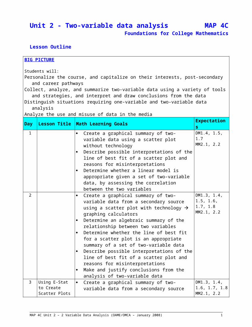
Unit 2 - Two-variable data analysis MAP 4CFoundations for College Mathematics

Lesson Outline

BIG PICTURE

Students will:Personalize the course, and capitalize on their interests, post-secondary and career pathwaysCollect, analyze, and summarize two-variable data using a variety of tools and strategies, and interpret and

draw conclusions from the dataDistinguish situations requiring one-variable and two-variable data analysisAnalyze the use and misuse of data in the mediaDay Lesson Title Math Learning Goals Expectations

1 Create a graphical summary of two-variable data using a scatter plot without technology

Describe possible interpretations of the line of best fit of a scatter plot and reasons for misinterpretations

Determine whether a linear model is appropriate given a set of two-variable data, by assessing the correlation between the two variables

DM1.4, 1.5, 1.7MM2.1, 2.2

2 Create a graphical summary of two-variable data from a secondary source using a scatter plot with technology graphing calculators

Determine an algebraic summary of the relationship between two variables

Determine whether the line of best fit for a scatter plot is an appropriate summary of a set of two-variable data


Make and justify conclusions from the analysis of two-variable data

DM1.3, 1.4, 1.5, 1.6, 1.7, 1.8MM2.1, 2.2

3 Using E-Stat to Create Scatter Plots and Lines of Best Fit

Lesson Included *New Jan/08*

Create a graphical summary of two-variable data from a secondary source using a scatter plot with technology Statistics Canada’s E-STAT

Determine whether the line of best fit for a scatter plot is an appropriate summary of a set of two-variable data



DM1.3, 1.4, 1.6, 1.7, 1.8MM2.1, 2.2

4 Jazz Day5 Determine an algebraic summary of the relationship

between two variables that appear to be linearly related and solve related problems (interpolate/extrapolate)

DM1.5

6 Indices


Describe examples of indices used by the media and solve problems by interpreting and using indices

DM2.2MM2.1, 2.2

7-8 Using Fathom to create scatter plots

Use data available from Census at School (secondary source) and technology (Fathom) in order to summarize

DM1.3, 1.4, 1.5, 1.6, 1.7, 1.8

MAP 4C Unit 2 – 2 Variable Data Analysis (OAME/OMCA – January 2008) 1

and Lines of Best Fit


properties (e.g. dependent and independent variables, line of best fit, correlation, etc.)

Determine an algebraic summary of the relationship between two variables and solve related problems


MM2.1, 2.2

9 Jazz Day10 Analysing Two-

Variable Data

Lesson Included *New Jan/08**M.O.

Summative Activity


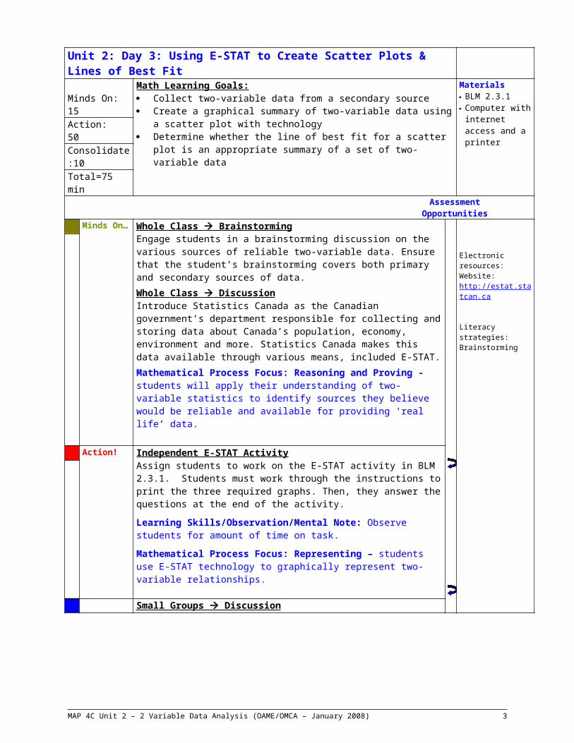
Unit 2: Day 3: Using E-STAT to Create Scatter Plots & Lines of Best Fit

Minds On: 15Math Learning Goals: Collect two-variable data from a secondary source Create a graphical summary of two-variable data using a scatter plot with

technology Determine whether the line of best fit for a scatter plot is an appropriate

summary of a set of two-variable data

Materials BLM 2.3.1 Computer with

internet access and a printerAction: 50

Consolidate:10

Total=75 minAssessment

OpportunitiesMinds On… Whole Class Brainstorming

Engage students in a brainstorming discussion on the various sources of reliable two-variable data. Ensure that the student’s brainstorming covers both primary and secondary sources of data.Whole Class Discussion Introduce Statistics Canada as the Canadian government’s department responsible for collecting and storing data about Canada’s population, economy, environment and more. Statistics Canada makes this data available through various means, included E-STAT.Mathematical Process Focus: Reasoning and Proving - students will apply their understanding of two-variable statistics to identify sources they believe would be reliable and available for providing ‘real life’ data.

Electronic resources: Website: http://estat.statcan.ca

Literacy strategies:Brainstorming

Action! Independent E-STAT ActivityAssign students to work on the E-STAT activity in BLM 2.3.1. Students must work through the instructions to print the three required graphs. Then, they answer the questions at the end of the activity.

Learning Skills/Observation/Mental Note: Observe students for amount of time on task.

Mathematical Process Focus: Representing – students use E-STAT technology to graphically represent two-variable relationships.

Consolidate Debrief

Small Groups Discussion Draw the attention of students to the three questions at the end of the activity. Divide students into small groups and have them discuss possible answers to the questions.

Expectations/Observation/Verbal Feedback: Circulate to all groups to assess their learning. Do students understand? Clarify misunderstandings with the whole class as needed.

ExplorationApplicationReflection

Home Activity or Further Classroom ConsolidationComplete the three required graphs at home if they are not yet complete. Complete the three questions at the end of the activity.

Students need an E-STAT ID and password to access from home. School boards usually have one ID and password that is used by all students.


http://estat.statcan.ca/

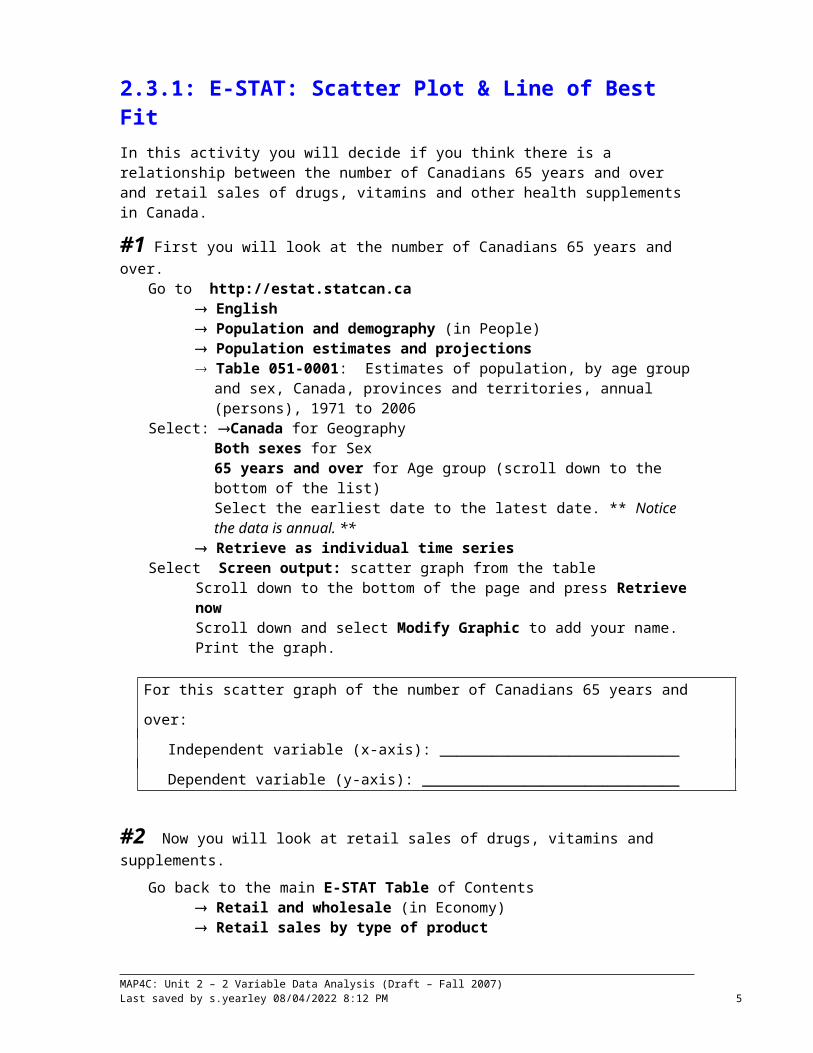
2.3.1: E-STAT: Scatter Plot & Line of Best FitIn this activity you will decide if you think there is a relationship between the number of Canadians 65 years and over and retail sales of drugs, vitamins and other health supplements in Canada.

#1 First you will look at the number of Canadians 65 years and over.Go to http://estat.statcan.ca

English Population and demography (in People) Population estimates and projections Table 051-0001: Estimates of population, by age group and sex, Canada,

provinces and territories, annual (persons), 1971 to 2006Select: Canada for Geography

Both sexes for Sex65 years and over for Age group (scroll down to the bottom of the list)Select the earliest date to the latest date. ** Notice the data is annual. **

Retrieve as individual time seriesSelect Screen output: scatter graph from the table

Scroll down to the bottom of the page and press Retrieve nowScroll down and select Modify Graphic to add your name. Print the graph.

For this scatter graph of the number of Canadians 65 years and over:

Independent variable (x-axis): _______________________________________

Dependent variable (y-axis): _________________________________________

#2 Now you will look at retail sales of drugs, vitamins and supplements.

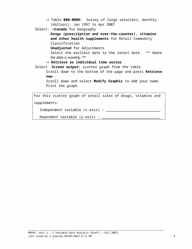
Go back to the main E-STAT Table of Contents Retail and wholesale (in Economy) Retail sales by type of product Table 080-0009: Survey of large retailers, monthly (dollars), Jan 1997 to

Apr 2007Select: Canada for Geography

Drugs (prescription and over-the-counter), vitamins and other health supplements for Retail Commodity ClassificationUnadjusted for AdjustmentsSelect the earliest date to the latest date. ** Notice the data is monthly. **

Retrieve as individual time seriesSelect Screen output: scatter graph from the table

Scroll down to the bottom of the page and press Retrieve nowScroll down and select Modify Graphic to add your name. Print the graph.

For this scatter graph of retail sales of drugs, vitamins and supplements:

Independent variable (x-axis) : _______________________________________

Dependent variable (y-axis) : ________________________________________

MAP4C: Unit 2 – 2 Variable Data Analysis (Draft – Fall 2007)Last saved by C Chilvers 19/05/2023 11:08 AM 4

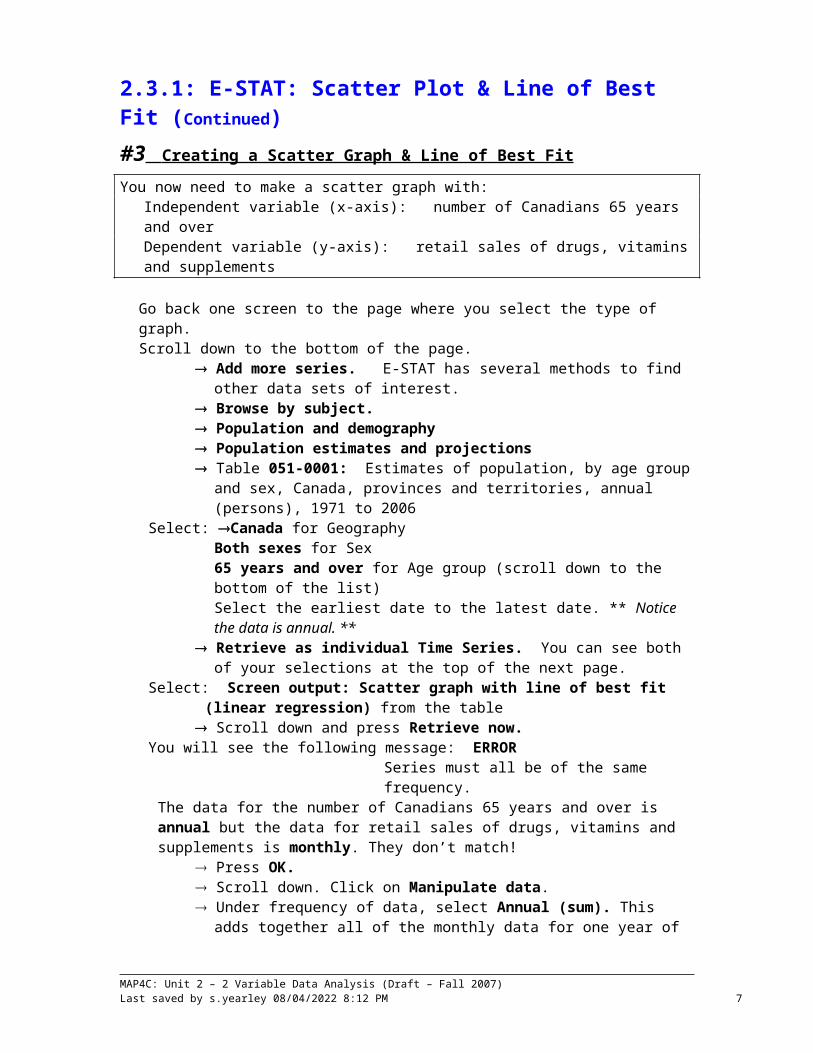
2.3.1: E-STAT: Scatter Plot & Line of Best Fit (Continued)#3 Creating a Scatter Graph & Line of Best Fit You now need to make a scatter graph with:

Independent variable (x-axis): number of Canadians 65 years and overDependent variable (y-axis): retail sales of drugs, vitamins and supplements

Go back one screen to the page where you select the type of graph.Scroll down to the bottom of the page.

Add more series. E-STAT has several methods to find other data sets of interest.

Browse by subject. Population and demography Population estimates and projections Table 051-0001: Estimates of population, by age group and sex, Canada,

provinces and territories, annual (persons), 1971 to 2006Select: Canada for Geography

Both sexes for Sex65 years and over for Age group (scroll down to the bottom of the list)Select the earliest date to the latest date. ** Notice the data is annual. **

Retrieve as individual Time Series. You can see both of your selections at the top of the next page.

Select: Screen output: Scatter graph with line of best fit (linear regression) from the table

Scroll down and press Retrieve now.You will see the following message: ERROR

Series must all be of the same frequency.The data for the number of Canadians 65 years and over is annual but the data for retail sales of drugs, vitamins and supplements is monthly. They don’t match!

Press OK. Scroll down. Click on Manipulate data. Under frequency of data, select Annual (sum). This adds together all of

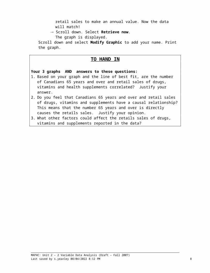
the monthly data for one year of retail sales to make an annual value. Now the data will match!

Scroll down. Select Retrieve now.The graph is displayed.

Scroll down and select Modify Graphic to add your name. Print the graph.

TO HAND IN

Your 3 graphs AND answers to these questions:1. Based on your graph and the line of best fit, are the number of Canadians 65 years

and over and retail sales of drugs, vitamins and health supplements correlated? Justify your answer.

2. Do you feel that Canadians 65 years and over and retail sales of drugs, vitamins and supplements have a causal relationship? This means that the number 65 years and over is directly causes the retails sales. Justify your opinion.

3. What other factors could affect the retails sales of drugs, vitamins and supplements reported in the data?


Unit 2: Day 6: Indices

Minds On: 15Math Learning Goals: Analyze graphs representing indices and use them to make predictions Determine how indices relate to everyday life

Materials BLM 2..6.1-2.6.5

Action: 55Consolidate: 5Total=75 min

AssessmentOpportunities

Minds On… Whole Class Discussion Lead students in a discussion about the concept of inflation. Introduce the Consumer Price Index as a measure of inflation and indices in general. Pair/Share Brainstorming Hand out the article from BLM 2.6.1 and ask students to read. Students should list the different consumer products from the article that are measured by the CPI. Then ask the students list and to reflect on the following:

the way in which inflation reflects their lives or their families’ lives the way that inflation will influence their future decisions why the CPI may not reflect their personal consumer experiences

Expectations/Observation/Anecdotal comments: Circulate while students discuss Inflation and the CPI and give them feedback and encouragement. Also monitor whether or not further class discussion is needed.

Your Guide to the Consumer Price Index can be found at http://www.statcan.ca/english/freepub/62-557-XIB/62-557-XIB1996001.pdf

Point out that the CPI is a measures the inflation across Canada.

Action! Whole Class Discussion Show the historical graph of the CPI from BLM 2.6.2 and discuss the important dates listed below the graph, as well as what factors affect the CPI. Point out that it is impossible to summarize the information on the graph over such a long period of time. Whole Class Teacher Directed Lesson Distribute and work through BLM 2.6.3 with the students on an overhead. Individual Activity Handout BLM 2.6.4 and introduce the New Housing Price Index as one component of the CPI. Ask students to reflect on how the New Housing Price Index may affect their lives in the future. Have students complete BLM 2.6.4 using BLM 2.6.3 as reference.Mathematical Process Focus: Reflecting– students will reflect on how the CPI and the New Housing Price Index will affect their lives.

Consolidate Debrief

Whole Class Teacher Directed Take up BLM 2.6.4 and ask the students to consider how the New Housing Price Index will affect their lives in the future.

ExplorationReflection

Home Activity or Further Classroom ConsolidationLists way in which you can prepare for the increase in housing prices and why a house may be a good investment or a bad investment. Complete BLM 2.6.5 for homework.


http://www.statcan.ca/english/freepub/62-557-XIB/62-557-XIB1996001.pdf



2.6.1 Inflation Article

Inflation eases to 2.2% but core inflation jumps to 4-year highLast Updated: Thursday, May 17, 2007 | 11:45 AM ET

http://www.cbc.ca/money/story/2007/05/17/inflation-april.html

CBC News

Canada's annual inflation rate edged down to 2.2 percent in April from 2.3 percent the month before, Statistics Canada reported Thursday. Analysts had expected inflation to come in a touch lower at 2.1 percent. But the core inflation rate — which excludes volatile items in the consumer price index — rose to 2.5 percent from 2.3 percent in March. That's its highest level in more than four years. Analysts noted that the upward pressure on core inflation was broadly based, suggesting that interest rate hikes may come later this year.

"The Bank of Canada … will probably be forced to acknowledge the growing upside risk to inflation with an eye to possible rate hikes in the future," said TD economist David Tulk. The Canadian dollar jumped almost half a cent to 91.05 cents US in late morning trading.

The year-over-year rise in the cost of living was driven by increases in housing costs, as prices for new homes rose and consumers paid more in mortgage interest. Gasoline, for once, wasn't a major culprit in the annual inflation rate, as prices at the pump were actually lower in April than they were a year earlier. Natural gas was also cheaper year-over-year, as were computers and video equipment. Food, however, costs more. Consumers paid 3.8 percent more for food than they did in April 2006. Fresh vegetables were 12.9 percent more expensive.

Alberta's housing boom once again gave it the dubious honour of having the highest inflation rate in the country — 5.5 percent. Homeowners' replacement costs in that province have shot up by more than 29 percent in the past year.

On a month-over-month basis, prices rose 0.4 percent from March to April — a marked slowdown from the 0.8 percent rise seen in the previous month. Prices for gasoline and natural gas rose in April; prices for non-alcoholic beverages and women's clothing fell.


http://www.cbc.ca/news/credit.html

2.6.1 Inflation Article (Teacher Notes)

Consumer Price Index Definition

The CPI is defined as an indicator of the changes in consumer prices experienced by Canadians. It is obtained by comparing, through time, the cost of a fixed basket of commodities purchased by Canadian consumers in a particular year. Since the basket contains commodities of unchanging or equivalent quantity and quality, the index reflects only pure price movements.

The CPI is one of many price change measures available to the public. It reflects the experience of Canadian consumers buying consumer goods and services.

It is important, however, to understand that the CPI measures the average change in retail prices encountered by all consumers in Canada.

Over 600 items representative of typical Canadian purchases are included in the CPI’s basket of goods and services. Major groupings include: 1. Food2. Shelter3. Household operations and furnishings4. Clothing and footwear5. Transportation6. Health and personal care7. Recreation, education and reading8. Alcoholic beverages and tobacco products


2.6.2 Historical Graph of CPI in Canada

1------------World War I2------------Recession3------------Great Depression4------------Recession in the U.S.A5------------World War II6------------Price Controls7------------Explosion of Pent-up Demand8------------Korean War9------------Credit Controls

10------------Period of Sustained Growth11------------First Oil Crisis12------------Anti-inflation Board13------------Second Oil Crisis14------------Wage Controls and Recession15------------Goods and Services Tax (GST)16------------Cigarette Tax Reduction

Obtained from: Your Guide to the Consumer Price Index (http://www.statcan.ca/english/freepub/62-557-XIB/62-557-XIB1996001.pdf)


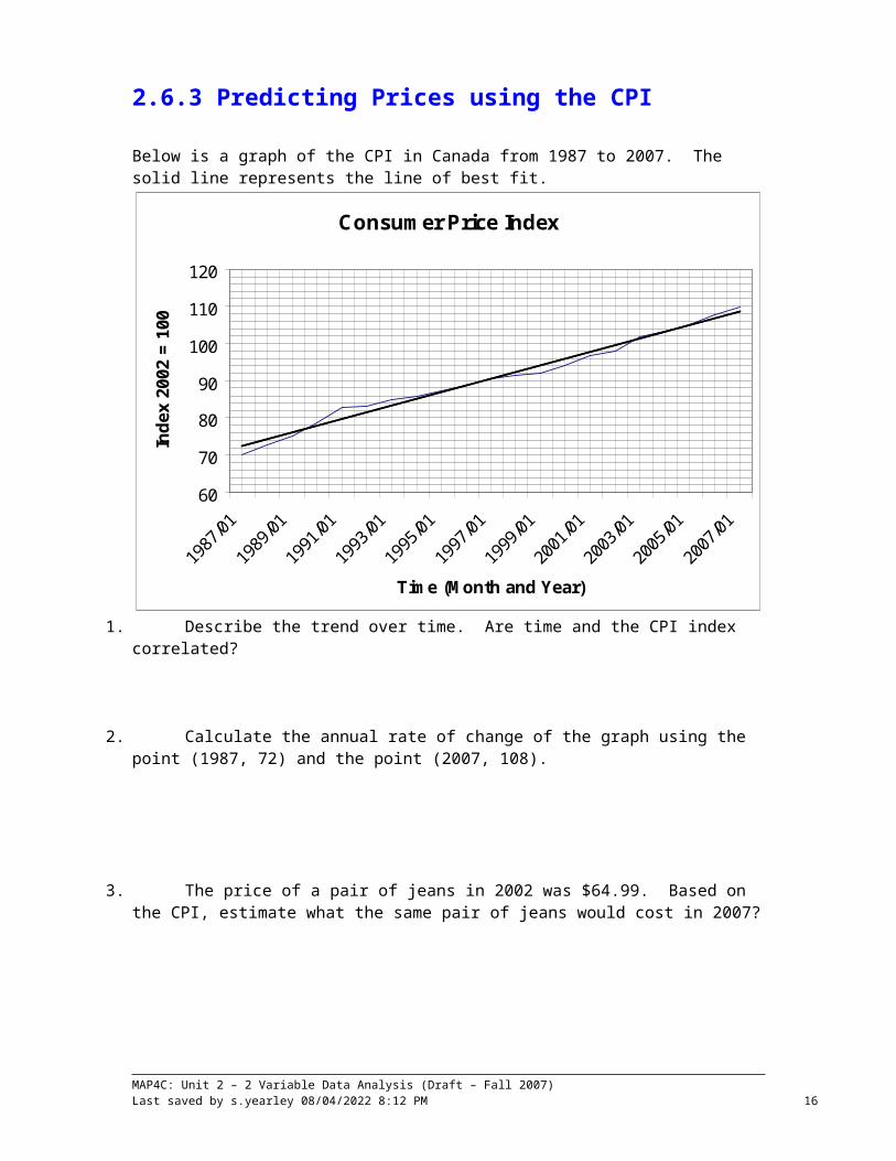
2.6.3 Predicting Prices using the CPI

Below is a graph of the CPI in Canada from 1987 to 2007. The solid line represents the line of best fit.

Consumer Price Index

60

70

80

90

100

110

120

1987

/01

1989

/01

1991

/01

1993

/01

1995

/01

1997

/01

1999

/01

2001

/01

2003

/01

2005

/01

2007

/01

Time (Month and Year)

Inde

x 20

02 =

100

1. Describe the trend over time. Are time and the CPI index correlated?

2. Calculate the annual rate of change of the graph using the point (1987, 72) and the point (2007, 108).

3. The price of a pair of jeans in 2002 was $64.99. Based on the CPI, estimate what the same pair of jeans would cost in 2007?

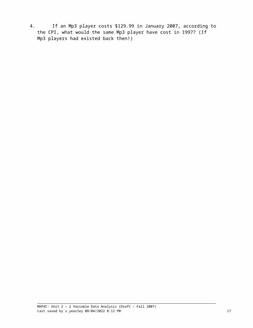
4. If an Mp3 player costs $129.99 in January 2007, according to the CPI, what would the same Mp3 player have cost in 1997? (If Mp3 players had existed back then!)


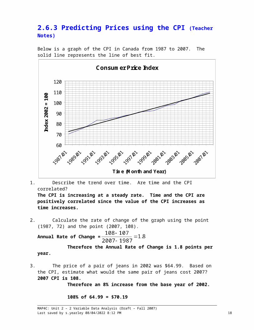
2.6.3 Predicting Prices using the CPI (Teacher Notes)

Below is a graph of the CPI in Canada from 1987 to 2007. The solid line represents the line of best fit.

Consumer Price Index

60

70

80

90

100

110

120

1987

/01

1989

/01

1991

/01

1993

/01

1995

/01

1997

/01

1999

/01

2001

/01

2003

/01

2005

/01

2007

/01

Time (Month and Year)

Inde

x 20

02 =

100

1. Describe the trend over time. Are time and the CPI correlated?The CPI is increasing at a steady rate. Time and the CPI are positively correlated since the value of the CPI increases as time increases.

2. Calculate the rate of change of the graph using the point (1987, 72) and the point (2007, 108).

Annual Rate of Change =

Therefore the Annual Rate of Change is 1.8 points per year.

3. The price of a pair of jeans in 2002 was $64.99. Based on the CPI, estimate what would the same pair of jeans cost 2007? 2007 CPI is 108.

Therefore an 8% increase from the base year of 2002.

108% of 64.99 = $70.19

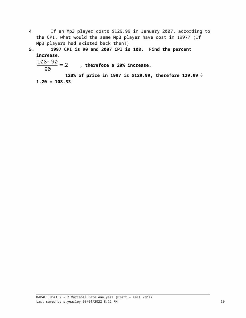
4. If an Mp3 player costs $129.99 in January 2007, according to the CPI, what would the same Mp3 player have cost in 1997? (If Mp3 players had existed back then!)

5. 1997 CPI is 90 and 2007 CPI is 108. Find the percent increase.

, therefore a 20% increase.

120% of price in 1997 is $129.99, therefore 129.99 1.20 = 108.33


2.6.4 The New Housing Price Index

Below is a graph and the data for the New Housing Price Index for Canada from January 1996 to January 2007.

New Housing Price Index

85

95

105

115

125

135

145

155

165

1996 1997 1998 1999 2000 2001 2002 2003 2004 2005 2006 2007

Year

Inde

x 19

97 =

100

Year Index 1996 981997 98.11998 102.41999 104.82000 108.22001 113.52002 117.62003 125.32004 133.92005 142.42006 148.32007 153.5

1. Find the mean of each variable and plot the point on the graph.

2. Draw a line of best fit on the graph above. Remember that the line must pass through the mean point .

3. Choose two points on the line of best fit and use them to determine the rate of change of the New Housing Price Index.


2.6.4 The New Housing (continued)

4. How does the annual rate of change in the New Housing Price Index compare to the annual rate of change for the CPI?

5. If I bought my house in 2004 for $140 000, based on the New Housing Price index, what would this house sell for if I sold it three years later in 2007?

6. If I bought my house in 1996 for $125 500, based on the New Housing Price Index, what would this house sell for if I sold it in 2003? In 2007?

7. If a house costs $250 000 in 2007, based on the New Housing Price Index, what would this house have sold for in 2000?

2.6.4 The New Housing Price Index (Teacher Notes)

Below is a graph and the data for the New Housing Price Index for Canada from January 1996 to January 2007.

New Housing Price Index

85

95

105

115

125

135

145

155

165

1996 1997 1998 1999 2000 2001 2002 2003 2004 2005 2006 2007

Year

Inde

x 19

97 =

100

Year Index 1996 981997 98.11998 102.41999 104.82000 108.22001 113.52002 117.62003 125.32004 133.92005 142.42006 148.32007 153.5

1. Find the mean of each variable and plot it on the graph .

2. Draw a line of best fit on the graph above. Remember that the line must pass through the mean point .

3. Choose two points on your line of best fit. Estimate the coordinates of these points and use them to determine the annual rate of change of the New Housing Price Index.

(2007,145) and (1998.5,105)

Annual Rate of Change Therefore the Annual Rate of Change is approx. 4.71 points per year.

2.6.4 The New Housing Price Index (Teacher Notes)

4. How does the annual rate of change for the New Housing Price Index compare to the annual rate of change for the CPI?

Based on the rate calculated in 3, the annual rate of change is much greater for the New Housing Price Index

5. If I bought my house in 2004 for $140 000, based on the New Housing Price Index, what would this house sell for if I sold it three years later in 2007?

2004 Index is 133.9 and 2007 Index is 153.5. Find the percent increase.

, therefore a 14.64% increase.

114.64% of price in 2004 is $140 000 x 1.1464 = 160 960

6. If I bought my house in 1996 for $125 500, based on the New Housing Price Index, what would this house sell for if I sold it in 2003? In 2007?

1996 Index is 98 and 2003 Index is 125.3. Find the percent increase.


127.86% of price in 1996 is $125 500 x 1.2786 = $160 464.30

1996 Index is 98 and 2007 Index is 153.5. Find the percent increase.


156.63% of price in 1996 is $125 500 x 1.5663 = $196 570.65

7. If a house costs $250 000 in 2007, based on the New Housing Price index, what would this house have sold for in 2000?

2000 Index is 108.2 and 2007 CPI is 153.5. Fnd the percent increase.


141.87% of price in 2000 is $250 000,therefore 250 000 141.87 = $176 217.66

2.6.5 How Much Can You Expect to PayBelow is the average New House Price for various cities in Canada.

Standard Two StoreyMarket Q1 2007 AverageHalifax 200,000

Charlottetown 175,000Moncton 132,000

Fredericton 187,000Saint John 210,400St. John's 200,000Atlantic 176,750

Montreal 338,857Ottawa 294,667Toronto 489,889

Winnipeg 220,714Regina 159,500

Saskatoon 257,500Calgary 411,456

Edmonton 384,750Vancouver 837,500

Victoria 418,000National 378,148

1. The New Housing Price Index in 2007 is 153.5. Use the rate of change from BLM 2.6.4 to predict what the New Housing Price Index will be in;

a. 5 years b. 10 years

2. Using the values calculated in question 1, calculate each percent increase from 2007;


3. From the list above, choose a city where you can see yourself living in 5 or 10 years. Use the average price for your city in 2007 and the information from questions 2 and 3 to calculate what you can expect to pay for a new house in;

a. 5years b. 10 years

4. How much will you need to save if you are going to make a 10% down payment?a. In 5 years b. In 10 years

Note: Average house prices are based on an average of all sub-markets examined in the area, except for the smaller markets of Charlottetown, Moncton, Fredericton, Saint John and Victoria.

FROM: http://www.royallepage.ca/CMSTemplates/AboutUs/Company/CompanyTemplate.aspx?id=1506

2.6.5 How Much Can You Expect to Pay (Teacher Notes)Below is the average New House Price for various cities in Canada.

Standard Two StoreyMarket Q1 2007 AverageHalifax 200,000

Charlottetown 175,000Moncton 132,000

Fredericton 187,000Saint John 210,400St. John's 200,000Atlantic 176,750

Montreal 338,857Ottawa 294,667Toronto 489,889

Winnipeg 220,714Regina 159,500

Saskatoon 257,500Calgary 411,456

Edmonton 384,750Vancouver 837,500

Victoria 418,000National 378,148

1. The New Housing Price Index in 2007 is 153.5. Use the rate of change from BLM 2.6.4 to predict what the New Housing Price Index will be in;

a. 5 years b. 10 years4.71 points per year 4.71 points per yearTherefore 5 x 4.71 =23.55 Therefore 10 x 4.71 =47.10153.5 + 23.55 = 177.05 153.5 + 47.10 = 200.6

2. Using the values calculated in question 1, calculate each percent increase from 2007;


15.34% 30.68%

3. From the list above, choose a city where you can see yourself living in 5 or 10 years. Use the average price for your city in 2007 and the information from questions 2 and 3 to calculate what you can expect to pay for a new house in;

a. 5years b. 10 years

Toronto $489,889 Therefore $489 889 x 1.3068 Therefore $489 889 x 1.1539 =$565 282.92 =$640 186.95

4. How much will you need to save if you are going to make a 10% down payment?a. 5 years b. 10 years

10% of $565 282.92 is $569 528.29 10% of $640 186.95 is $64 018.70

Note: Average house prices are based on an average of all sub-markets examined in the area, except for the smaller markets of Charlottetown, Moncton, Fredericton, Saint John and Victoria.

FROM: http://www.royallepage.ca/CMSTemplates/AboutUs/Company/CompanyTemplate.aspx?id=1506

Unit 2: Days 7 & 8:Using Fathom to Create Scatter Plots & Lines of Best Fit

Minds On: 15Math Learning Goals: Use data available from Census at School (secondary source) and technology

(Fathom) in order to summarize properties (e.g. dependent and independent variables, line of best fit, correlation, etc.)

Determine an algebraic summary of the relationship between two variables and solve related problems


Materials BLM 2.7.1 Computer with

Fathom and a printer

Copies of current data printed from http://www19.statcan.ca/r000_e.htm

Action: 105

Consolidate:30

Total=150 minAssessment

OpportunitiesMinds On… Whole Class Discussion

Introduce the use of Census at School as a secondary source of data. Census at School data is gathered from students in participating classes across Canada and internationally. This activity uses data about Canadian boys.Ask the class to consider if the data gathered by the Census at School project can be used to interpolate/extrapolate values about all Canadian boys. Create a list of variables they predict can be calculated reliably using the Census at School data.Mathematical Process Focus: Reasoning and Proving – students will apply their understanding of two-variable statistics to make conjectures about the usefulness and reliability of the Census at School data.

You will need to copy a current set of the Census at School data from http://www19.statcan.ca/r000_e.htm for each student. When at the Census at School site, look for Canadian results – Canadian summary tables. Print Average height by age, Average length of forearm by age, Average length of hand by age, Average length of foot by age.

Assessment ‘as’ learning strategy:Self evaluation of solutions

Students who complete their work early can be encouraged to choose 2 pieces of data from the census at school site that they think are related, download the data and test their hypothesis.

Action! Independent Fathom Activity Assign students to work on the Fathom activity in BLM 2.7.1. On Day 7, instruct students to follow the Part 1 instructions to create the required graph and then answer the questions that follow. On Day 8, students should complete Part 2 and Part 3.Learning Skills/Observation/Mental Note: Observe students for amount of time on task.

Mathematical Process Focus: Representing – Students use Fathom technology to graphically represent two-variable relationships.

Consolidate Debrief

Small Groups Discussion At the end of each day, divide students into small groups and have them compare answers to the questions. Student should identify differing answers and verify their solutions by checking their data and their calculations. They should make corrections as needed.

Expectations/Presentation/Verbal Feedback: Circulate to all groups to assess their learning. Do students understand? Clarify misunderstandings and “problem” questions with the whole class as needed.

Application

Differentiated

Home Activity or Further Classroom ConsolidationComplete the interpolation and extrapolation calculations at home, if you have not completed them yet.

If you have completed today’s activity: Create 5 new questions that require interpolation/extrapolation. Exchange your questions with another student. Then, trade solutions and correct the answers.

http://www19.statcan.ca/r000_e.htm




2.7.1: Fathom & Line of Best FitThis activity introduces you to a software package called Fathom. You will use Fathom and some data from Census at School to determine the equation of a line of best fit and then use it to interpolate and extrapolate measurements for boys.

PART 1: Hand Length vs. Height1. Launch Fathom.2. Create a case table: Data is stored in a case table. Move your cursor over the table icon on

the main toolbar. Click on the table and drag it onto the main document.3. Enter the variable name: Click on the word <new> and type the word “hand_length”

instead. Repeat this in the next cell to replace <new> with “height”.4. Enter the data: In the “hand_length” column, enter the data in order from youngest to oldest

for the hand length of the boys. In the “height” column, enter the data in order from youngest to oldest for the height of the boys. The hand length and height of each age should be side-by-side in the table.

5. Drag a graph on the document: Move your cursor over the graph icon on the main toolbar. Click on the graph and drag it onto a blank space in the main document.

6. Graph the data: To create a scatter plot with hand length as the independent variable and height as the dependent variable, first click on “hand_length” in the case table and drag it onto the graph’s x-axis. Then, click on “height” in the case table and drag it onto the graph’s y-axis. Fathom will automatically create the scatter plot.

7. Create the least-squares line (line of best fit): Right-mouse-click in the graph to open a drop-down menu. Select “least-squares line” from the menu. Fathom will create the line of best fit on the graph, and display the equation of the line below the graph.

8. Arrange the data and graph on the page so it will print properly on a single sheet of paper. Leave space at the bottom of the page to answer the questions below.

9. Add your name in a text box.10. Print.

Now use the equation of the line of best fit to answer these questions. You must show your work! You may answer the questions neatly on the page you just printed.

a. Describe the correlation of the hand length and height of boys.b. Is the line of best fit a good fit for the data? Justify your answer.c. Interpolate the height of a boy with a hand length of 15.0 cm.d. Interpolate the hand length of a boy who is 162 cm tall.e. Extrapolate the height of a boy with a hand length of 6cm. Does this seem realistic?f. Extrapolate the height of a boy with a hand length of 20 cm. Does this seem realistic?g. Find Michael Jordan’s height in centimetres by searching on-line. Use this height to

extrapolate his hand length. Does this seem realistic?h. Is this line of best fit reliable for predicting hand lengths and heights of boys? Are

there any restrictions for using it?i. Why it is important to use only one gender (in this case, boys) when creating and

analyzing this scatter plot?

2.7.1: Fathom & Line of Best Fit (Continued)PART 2: Forearm Length vs. Foot Length 1. Open a new Fathom page.2. Repeat the steps in Part 1 to create a scatter plot with forearm length as the independent

variable and foot length as the dependent variable.3. Create the least-squares line (line of best fit).4. Arrange the data and graph on the page; add your name in a text box, and print.


a. Describe the correlation of the forearm length and foot length of boys.b. Is the line of best fit a good fit for the data? Justify your answer.c. Interpolate the foot length of a boy with a forearm length of 24.25 cm.d. Interpolate the forearm length of a boy with a foot length of 25 cm.e. Extrapolate the foot length of a boy with a forearm length of 30 cm. Does this seem

realistic?f. Extrapolate the forearm length of a boy with a foot length of 18 cm. Does this seem

realistic?g. Is this line of best fit reliable for predicting forearm lengths and foot lengths of boys?

Are there any restrictions for using it?

PART 3: Age vs. Height1. Open a new Fathom page.2. Create a scatter plot with age as the independent variable and height as the dependent

variable.3. Create the least-squares line (line of best fit).4. Arrange the data and graph on the page; add your name in a text box, and print.


a. Describe the correlation of the age and height of boys.b. Is the line of best fit a good fit for the data? Justify your answer.c. Interpolate the height of a boy who is 11½ years old.d. Interpolate the age of a boy with a height of 171 cm.e. Extrapolate the height of a boy who is 6 years old. Does this seem realistic? Why or

why not?f. Extrapolate the height of a boy who is 30 years old. Does this seem realistic? Why or

why not? g. Is this line of best fit reliable for predicting ages and heights of boys? Are there any

restrictions for using it?

2.7.2: Fathom & Line of Best Fit – Teacher Notes

Following is the data used for the 2007-2008 school year. It is the Canadian Census at School results for 2006-2007. The equation of each line of best fit as well as the interpolation and extrapolation answers are also provided for the 2006-2007 data.

***You will need to copy a current set of the Census at School data from http://www19.statcan.ca/r000_e.htm for each student. When at the Census at School site, look for Canadian results – Canadian summary tables. Print Average height by age, Average length

of forearm by age, Average length of hand by age, Average length of foot by age.***

PART 1: Hand Length vs. Height

Equation: height = 8.10 hand_length + 17.6Answers: c) 139.1 cm d) 17.8 cm e) 66.2 cm f) 179.6 cm

g) Using 198 cm gives 22.3 cm

**Note: 1. For Part “g) Find Michael Jordan’s height in centimetres by ...” You may wish to change Michael Jordan to another tall athlete that your class knows well.

2. For the other 2 parts, you may wish to have half of the class look at boys data and the other half look at girls data and have them compare the results. This may also help them answer i from Part 1


2.7.2: Fathom & Line of Best Fit – Teacher Notes (Continued)

PART 2: Forearm Length vs. Foot Length

Equation: foot length = 0.80 forearm + 4.1Answers: c) 23.5 cm d) 26.1 cm e) 28.1 cm f) 17.4 cm

PART 3: Age vs. Height

Equation: height = 4.40 age + 101.8Answers: c) 152.4 cm d) 15.7 cm e) 128.2 cm f) 233.8 cm

Documents

Unit x: Day x: Title · Web viewEnter the variable name: Click on the word and type the word “hand_length” instead. Repeat this in the next cell to replace