Embed Size (px)
Citation preview
Unit Two
Descriptive Biostatistics
Dr. Hamza Aduraidi
Biostatistics
What is the biostatistics? A branch of applied math. that deals with collecting, organizing and interpreting data using well-defined procedures.
Types of Biostatistics: Descriptive Statistics. It involves organizing,
summarizing & displaying data to make them more understandable.
Inferential Statistics. It reports the degree of confidence of the sample statistic that predicts the value of the population parameter.
Descriptive Biostatistics
The best way to work with data is to summarize and organize them.
Numbers that have not been summarized and organized are called raw data.
3
8 February 2019 4
Definition
Data is any type of information
Raw data is a data collected as they receive.
Organize data is data organized either in ascending, descending or in a grouped data.
Descriptive Measures
A descriptive measure is a single number that is used to describe a set of data.
Descriptive measures include measures of central tendencyand measures of dispersion.
5
Descriptive Measures Measures of Location
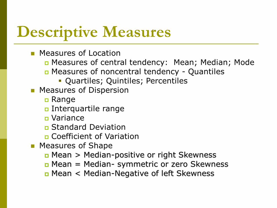
Measures of central tendency: Mean; Median; Mode Measures of noncentral tendency - Quantiles
Quartiles; Quintiles; Percentiles Measures of Dispersion
Range Interquartile range Variance Standard Deviation Coefficient of Variation
Measures of Shape Mean > Median-positive or right Skewness Mean = Median- symmetric or zero Skewness Mean < Median-Negative of left Skewness
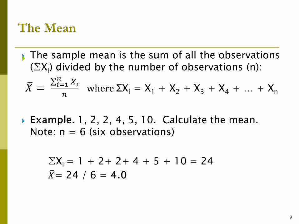
Measures of Location
It is a property of the data that they tend to be clustered about a center point.
Measures of central tendency (i.e., central location) help find the approximate center of the dataset.
Researchers usually do not use the term average, because there are three alternative types of average.
These include the mean, the median, and the mode. In a perfect world, the mean, median & mode would be the same.
mean (generally not part of the data set)
median (may be part of the data set)
mode (always part of the data set)
8
9
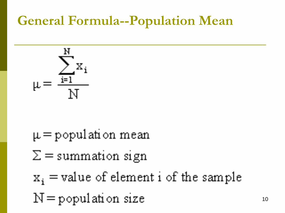
General Formula--Population Mean
10
8 February 2019 11
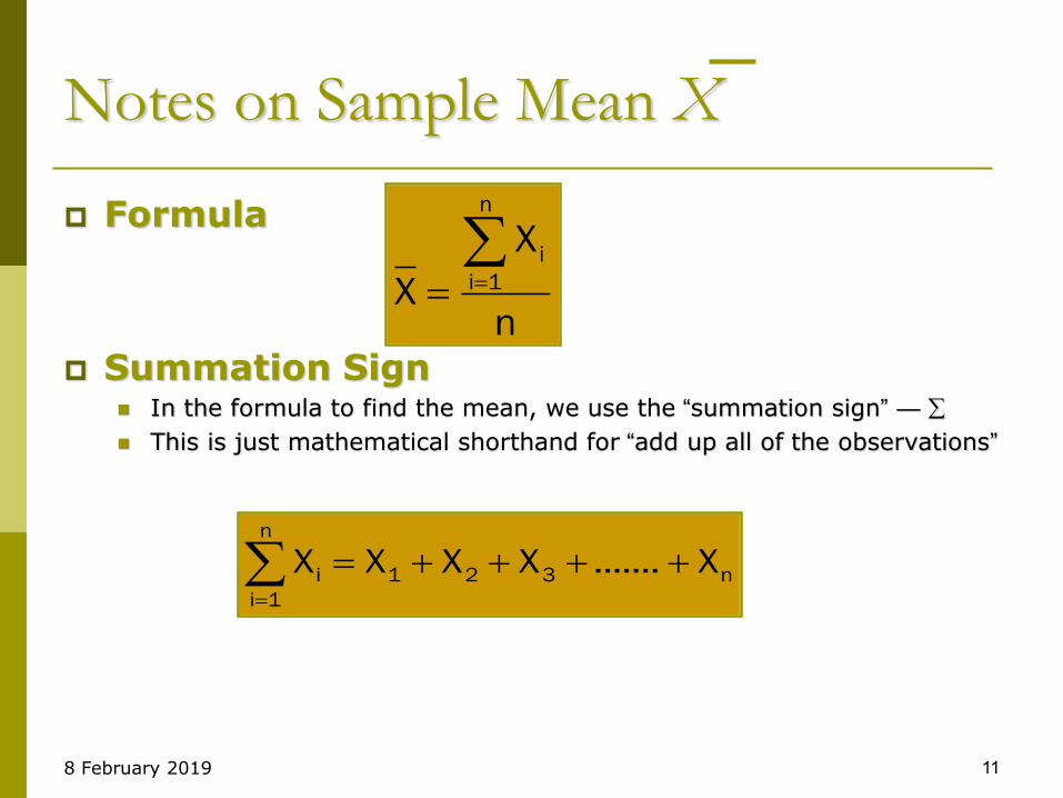
Notes on Sample Mean X
Formula
Summation Sign In the formula to find the mean, we use the “summation sign” —
This is just mathematical shorthand for “add up all of the observations”
n
X
X
n
1i
i
n321
n
1i
i X.......XXXX
8 February 2019 12
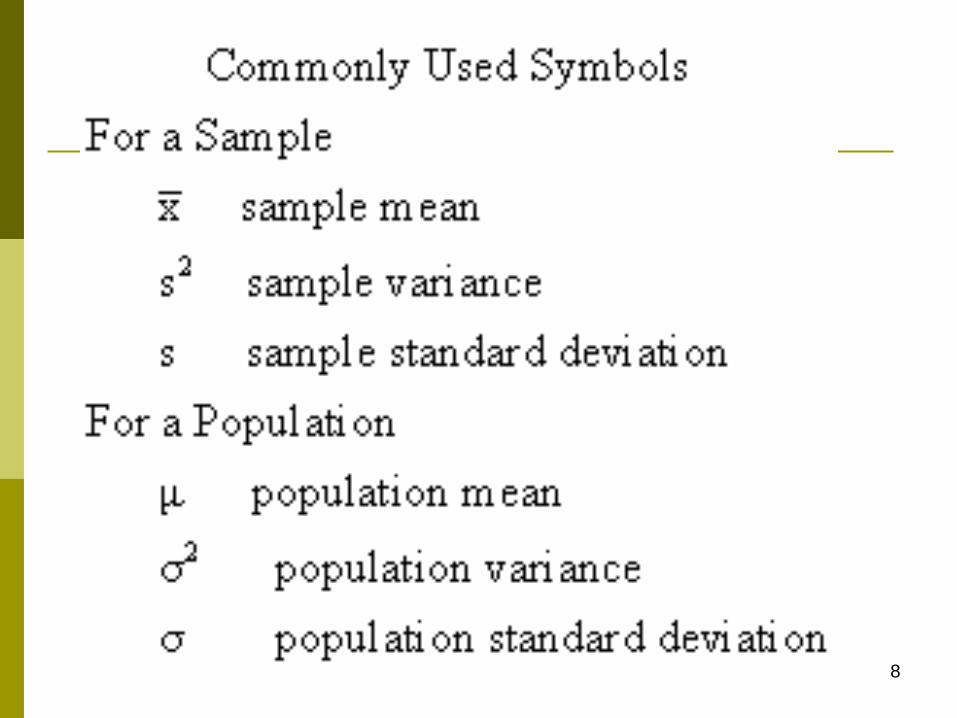
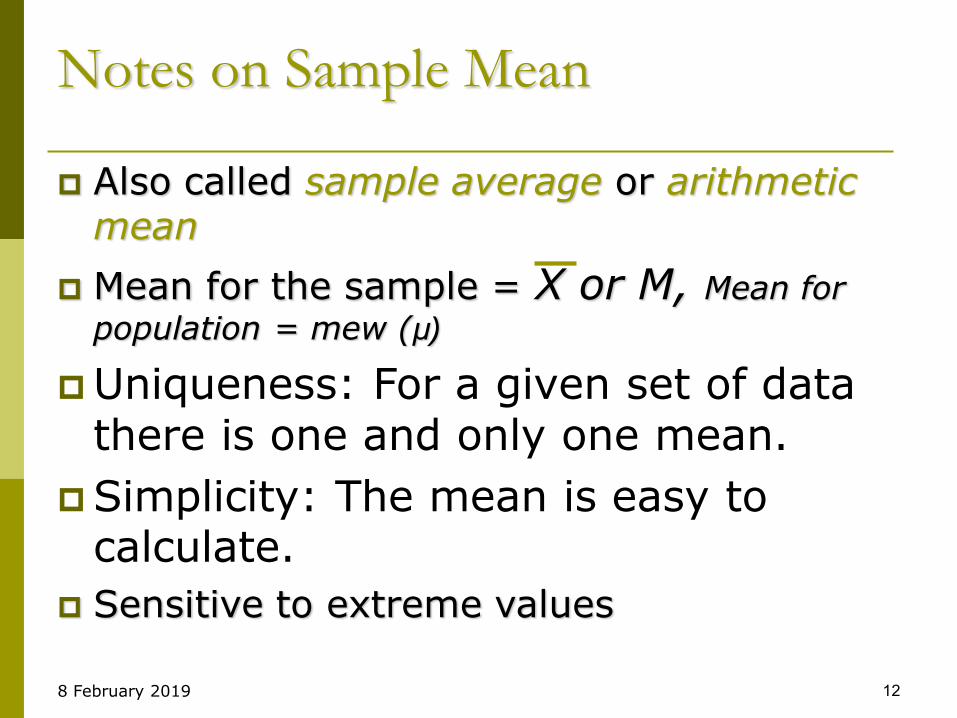
Notes on Sample Mean
Also called sample average or arithmetic mean
Mean for the sample = X or M, Mean for
population = mew (μ)
Uniqueness: For a given set of data there is one and only one mean.
Simplicity: The mean is easy to calculate.
Sensitive to extreme values
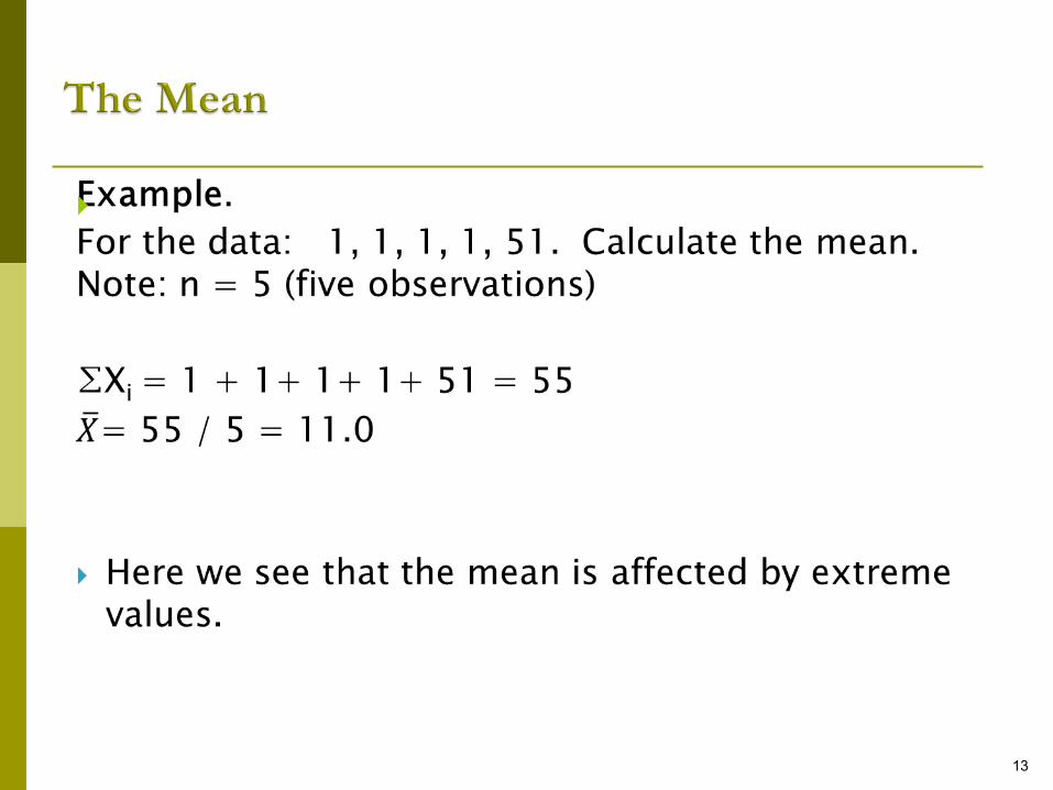
13
The median is the middle value of the ordered data
To get the median, we must first rearrange the data into an ordered array (in ascending or descending order). Generally, we order the data from the lowest value to the highest value.
Therefore, the median is the data value such that half of the observations are larger and half are smaller. It is also the 50th percentile.
If n is odd, the median is the middle observation of the ordered array. If n is even, it is midway between the two central observations.
14
Example:
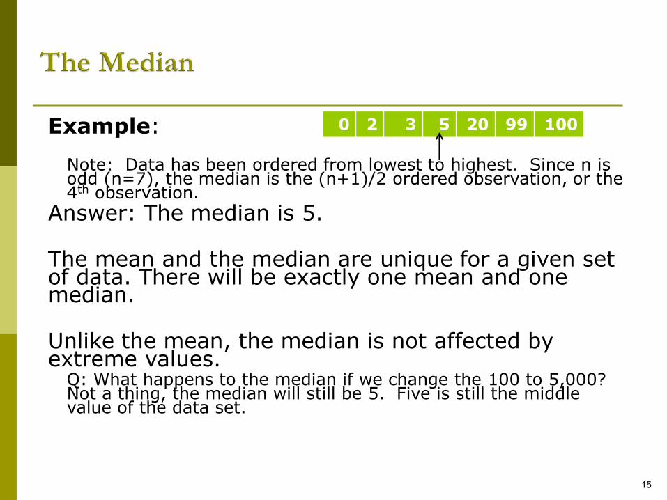
Note: Data has been ordered from lowest to highest. Since n is odd (n=7), the median is the (n+1)/2 ordered observation, or the 4th observation.
Answer: The median is 5.
The mean and the median are unique for a given set of data. There will be exactly one mean and one median.
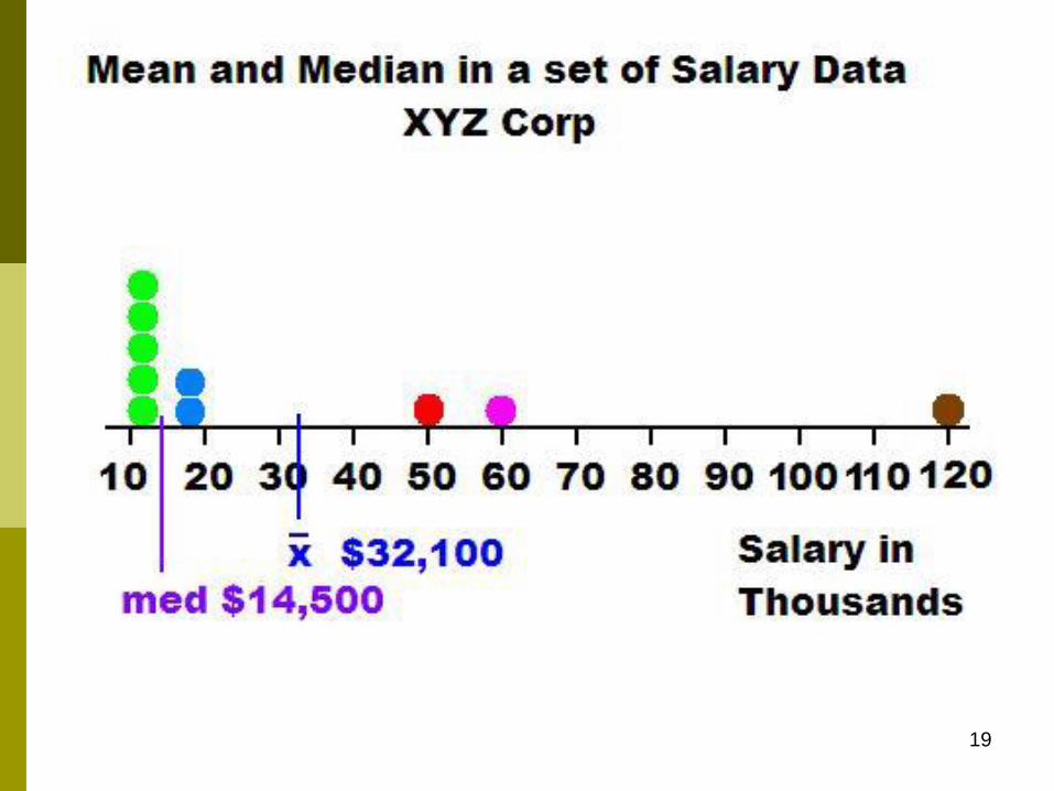
Unlike the mean, the median is not affected by extreme values.
Q: What happens to the median if we change the 100 to 5,000? Not a thing, the median will still be 5. Five is still the middle value of the data set.
15
0 2 3 5 20 99 100
Example:
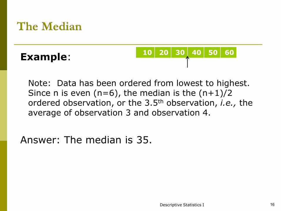
Note: Data has been ordered from lowest to highest. Since n is even (n=6), the median is the (n+1)/2 ordered observation, or the 3.5th observation, i.e., the average of observation 3 and observation 4.
Answer: The median is 35.
Descriptive Statistics I 16
10 20 30 40 50 60
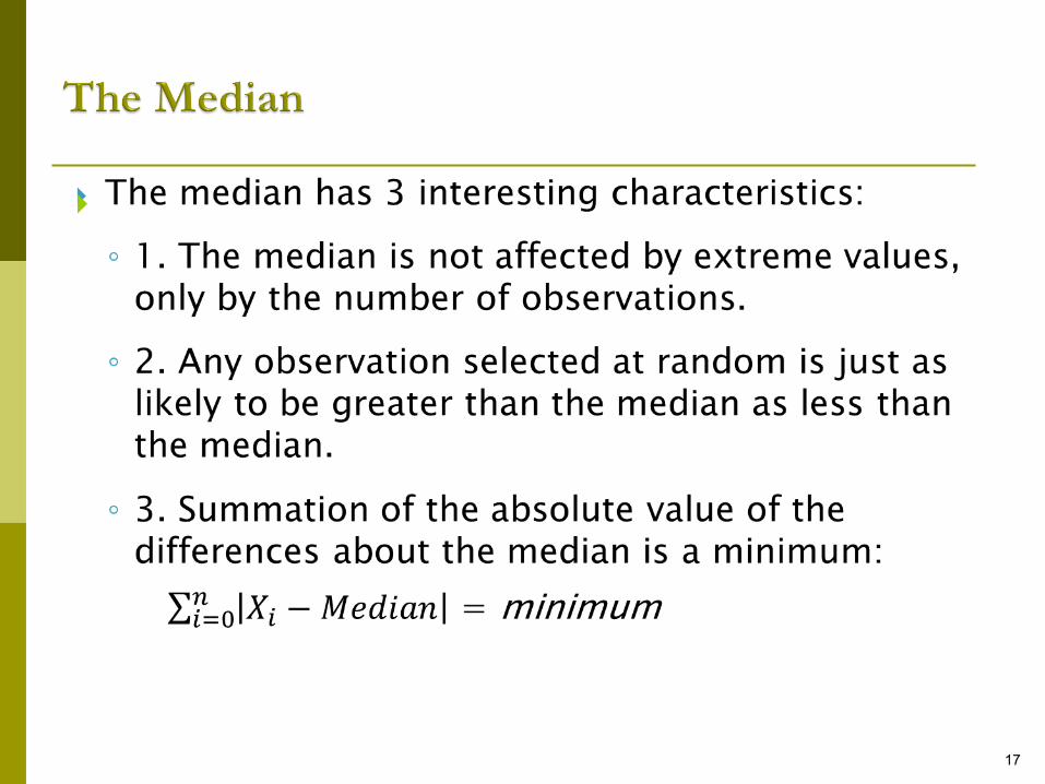
17
8 February 2019 18
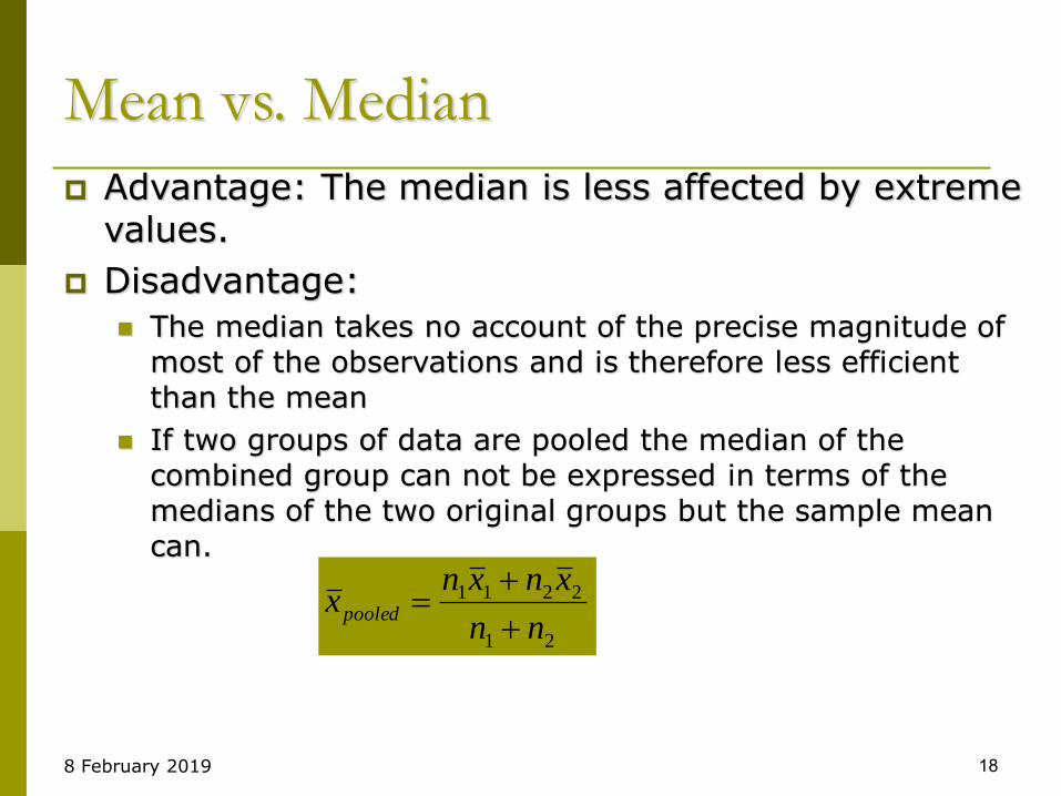
Mean vs. Median
Advantage: The median is less affected by extreme values.
Disadvantage:
The median takes no account of the precise magnitude of most of the observations and is therefore less efficient than the mean
If two groups of data are pooled the median of the combined group can not be expressed in terms of the medians of the two original groups but the sample mean can.
21
2211
nn
xnxnxpooled
19
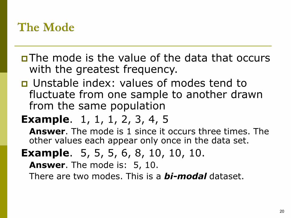
The mode is the value of the data that occurs with the greatest frequency.
Unstable index: values of modes tend to fluctuate from one sample to another drawn from the same population
Example. 1, 1, 1, 2, 3, 4, 5Answer. The mode is 1 since it occurs three times. The other values each appear only once in the data set.
Example. 5, 5, 5, 6, 8, 10, 10, 10.Answer. The mode is: 5, 10.
There are two modes. This is a bi-modal dataset.
20
The mode is different from the mean and the median in that those measures always exist and are always unique. For any numeric data set there will be one mean and one median.
The mode may not exist.
Data: 1, 2, 3, 4, 5, 6, 7, 8, 9, 0
Here you have 10 observations and they are all different.
The mode may not be unique.
Data: 0, 1, 1, 2, 2, 3, 3, 4, 4, 5, 5, 6, 6, 7
Mode = 1, 2, 3, 4, 5, and 6. There are sixmodes.
21
Comparison of the Mode, the Median,
and the Mean
In a normal distribution, the mode , the median, and the mean have the same value.
The mean is the widely reported index of central tendency for variables measured on an interval and ratio scale.
The mean takes each and every score into account.
It also the most stable index of central tendency and thus yields the most reliable estimate of the central tendency of the population.
Comparison of the Mode, the Median,
and the Mean
The mean is always pulled in the direction of the long tail, that is, in the direction of the extreme scores.
For the variables that positively skewed (like income), the mean is higher than the mode or the median. For negatively skewed variables (like age at death) the mean is lower.
When there are extreme values in the distribution (even if it is approximately normal), researchers sometimes report means that have been adjusted for outliers.
To adjust means one must discard a fixed percentage (5%) of the extreme values from either end of the distribution.
8 February 2019 24
Distribution Characteristics
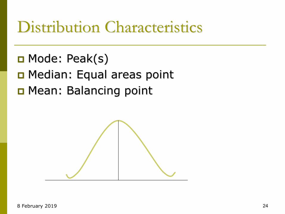
Mode: Peak(s)
Median: Equal areas point
Mean: Balancing point
8 February 2019 25
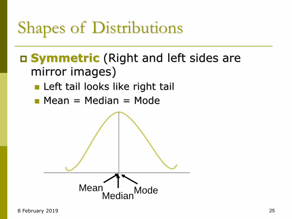
Shapes of Distributions
Symmetric (Right and left sides are mirror images)
Left tail looks like right tail
Mean = Median = Mode
MeanMedian
Mode
8 February 2019 26
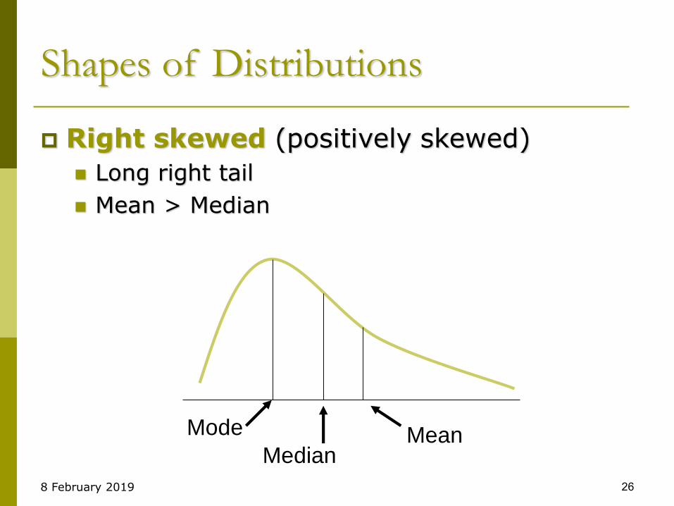
Shapes of Distributions
Right skewed (positively skewed)
Long right tail
Mean > Median
MeanMode
Median
8 February 2019 27
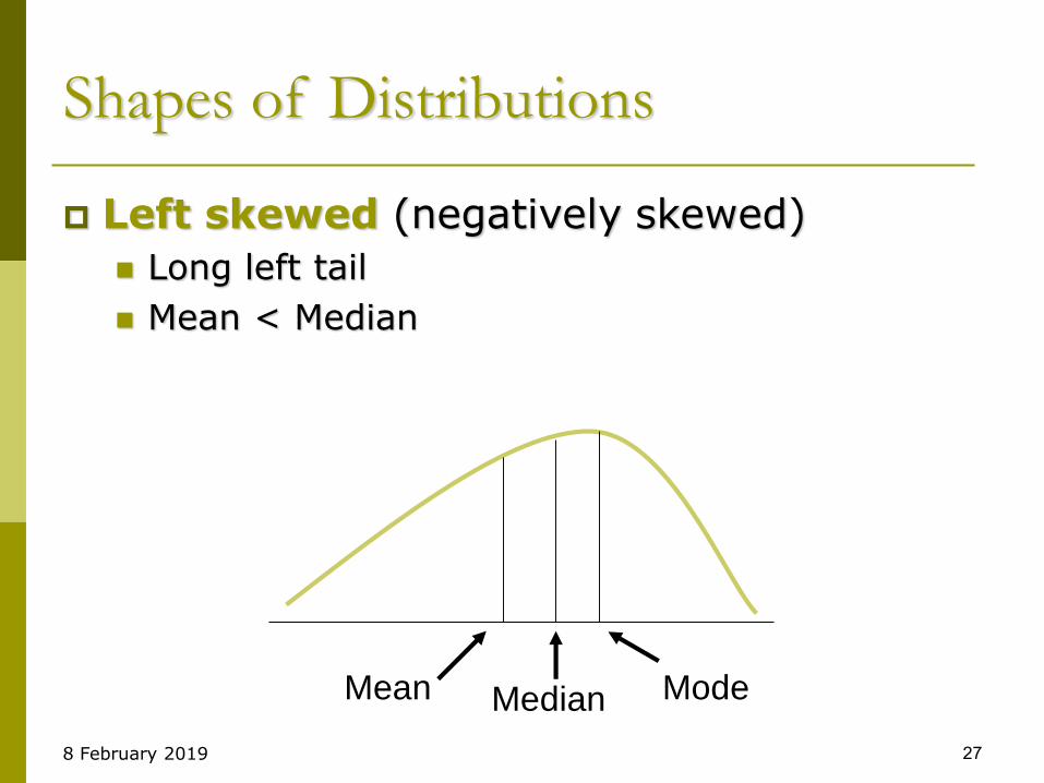
Shapes of Distributions
Left skewed (negatively skewed)
Long left tail
Mean < Median
ModeMedianMean
Measures of non-central location used to summarize a set of data
Examples of commonly used quantiles:
Quartiles
Quintiles
Deciles
Percentiles
Descriptive Statistics I 28
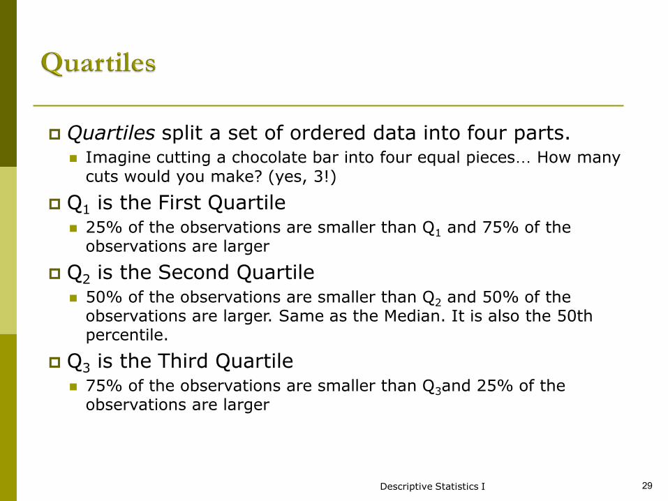
Quartiles split a set of ordered data into four parts. Imagine cutting a chocolate bar into four equal pieces… How many
cuts would you make? (yes, 3!)
Q1 is the First Quartile 25% of the observations are smaller than Q1 and 75% of the
observations are larger
Q2 is the Second Quartile 50% of the observations are smaller than Q2 and 50% of the
observations are larger. Same as the Median. It is also the 50th percentile.
Q3 is the Third Quartile 75% of the observations are smaller than Q3and 25% of the
observations are larger
Descriptive Statistics I 29
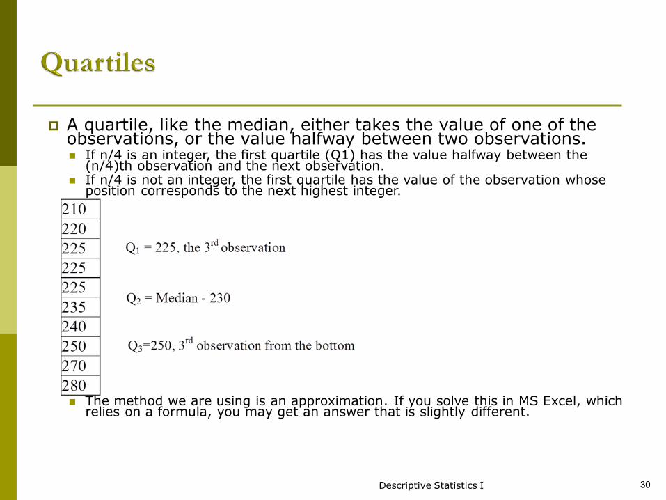
A quartile, like the median, either takes the value of one of the observations, or the value halfway between two observations. If n/4 is an integer, the first quartile (Q1) has the value halfway between the
(n/4)th observation and the next observation. If n/4 is not an integer, the first quartile has the value of the observation whose
position corresponds to the next highest integer.
The method we are using is an approximation. If you solve this in MS Excel, which relies on a formula, you may get an answer that is slightly different.
Descriptive Statistics I 30
31
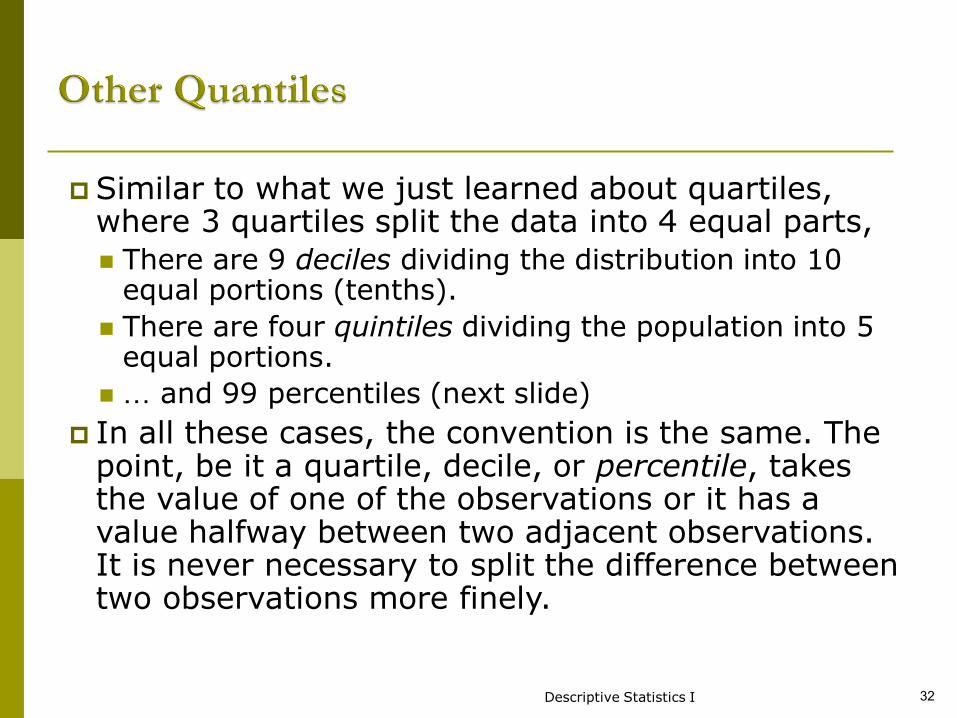
Similar to what we just learned about quartiles, where 3 quartiles split the data into 4 equal parts,
There are 9 deciles dividing the distribution into 10 equal portions (tenths).
There are four quintiles dividing the population into 5 equal portions.
… and 99 percentiles (next slide)
In all these cases, the convention is the same. The point, be it a quartile, decile, or percentile, takes the value of one of the observations or it has a value halfway between two adjacent observations. It is never necessary to split the difference between two observations more finely.
Descriptive Statistics I 32
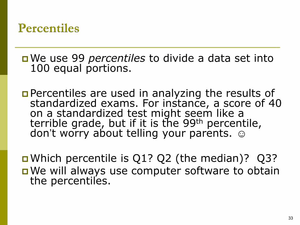
We use 99 percentiles to divide a data set into 100 equal portions.
Percentiles are used in analyzing the results of standardized exams. For instance, a score of 40 on a standardized test might seem like a terrible grade, but if it is the 99th percentile, don’t worry about telling your parents. ☺
Which percentile is Q1? Q2 (the median)? Q3?We will always use computer software to obtain
the percentiles.
33
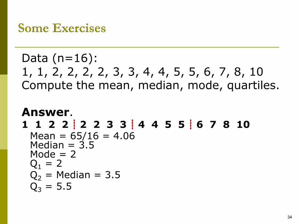
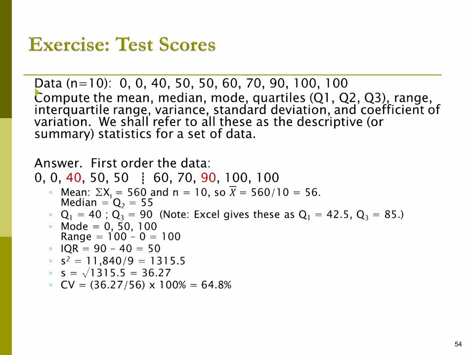
Data (n=16):1, 1, 2, 2, 2, 2, 3, 3, 4, 4, 5, 5, 6, 7, 8, 10Compute the mean, median, mode, quartiles.
Answer.1 1 2 2 ┋ 2 2 3 3 ┋ 4 4 5 5 ┋ 6 7 8 10
Mean = 65/16 = 4.06Median = 3.5Mode = 2Q1 = 2Q2 = Median = 3.5Q3 = 5.5
34
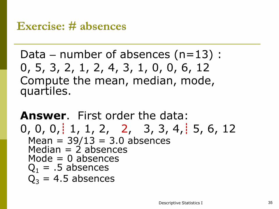
Data – number of absences (n=13) :0, 5, 3, 2, 1, 2, 4, 3, 1, 0, 0, 6, 12 Compute the mean, median, mode, quartiles.
Answer. First order the data:0, 0, 0,┋ 1, 1, 2, 2, 3, 3, 4,┋ 5, 6, 12
Mean = 39/13 = 3.0 absencesMedian = 2 absencesMode = 0 absencesQ1 = .5 absencesQ3 = 4.5 absences
Descriptive Statistics I 35
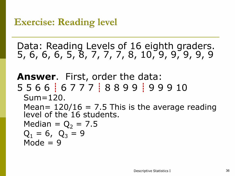
Data: Reading Levels of 16 eighth graders.5, 6, 6, 6, 5, 8, 7, 7, 7, 8, 10, 9, 9, 9, 9, 9
Answer. First, order the data:5 5 6 6 ┋ 6 7 7 7 ┋ 8 8 9 9 ┋ 9 9 9 10
Sum=120. Mean= 120/16 = 7.5 This is the average reading level of the 16 students.Median = Q2 = 7.5Q1 = 6, Q3 = 9Mode = 9
Descriptive Statistics I 36
It refers to how spread out the scores are.In other words, how similar or different
participants are from one another on the variable. It is either homogeneous or heterogeneous sample.
Why do we need to look at measures of dispersion?
Consider this example:A company is about to buy computer chips that must have an average life of 10 years. The company has a choice of two suppliers. Whose chips should they buy? They take a sample of 10 chips from each of the suppliers and test them. See the data on the next slide.
37
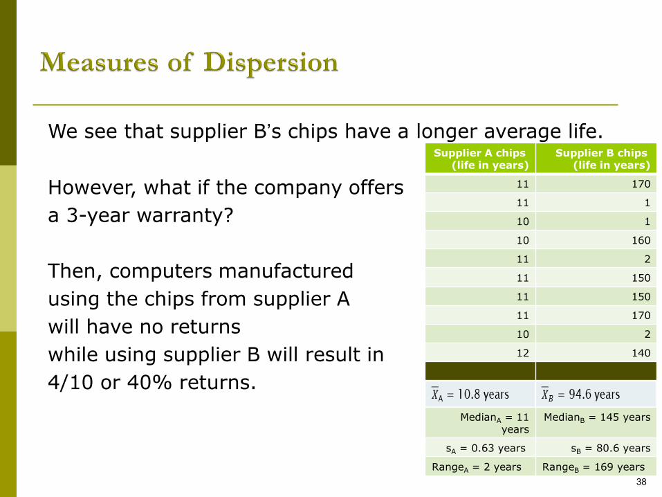
We see that supplier B’s chips have a longer average life.
However, what if the company offers
a 3-year warranty?
Then, computers manufactured
using the chips from supplier A
will have no returns
while using supplier B will result in
4/10 or 40% returns.
38
Supplier A chips (life in years)
Supplier B chips (life in years)
11 170
11 1
10 1
10 160
11 2
11 150
11 150
11 170
10 2
12 140
MedianA = 11 years
MedianB = 145 years
sA = 0.63 years sB = 80.6 years
RangeA = 2 years RangeB = 169 years
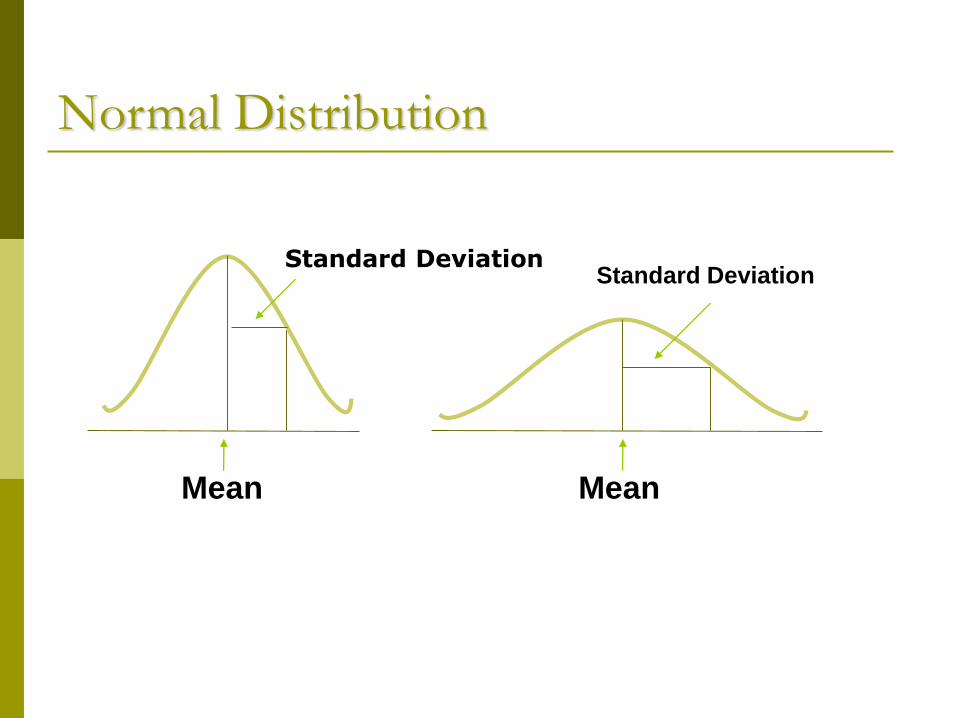
Normal Distribution
Mean
Standard DeviationStandard Deviation
Mean
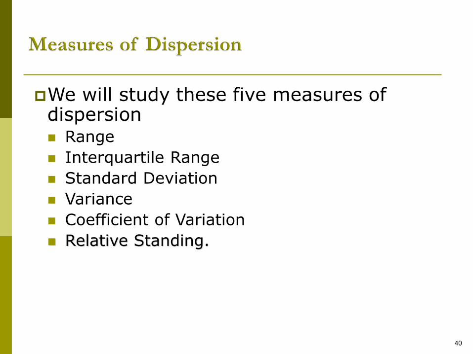
We will study these five measures of dispersion Range
Interquartile Range
Standard Deviation
Variance
Coefficient of Variation
Relative Standing.
40
The Range
Is the simplest measure of variability, is the difference between the highest score and the lowest score in the distribution.
In research, the range is often shown as the minimum and maximum value, without the abstracted difference score.
It provides a quick summary of a distribution’s variability.
It also provides useful information about a distribution when there are extreme values.
The range has two values, it is highly unstable.
Range = Largest Value – Smallest ValueExample: 1, 2, 3, 4, 5, 8, 9, 21, 25, 30
Answer: Range = 30 – 1 = 29.
Pros: Easy to calculate
Cons: Value of range is only determined by two
values
The interpretation of the range is difficult.
One problem with the range is that it is influenced by extreme values at either end.
42
43
Descriptive Statistics I 44
Standard Deviation
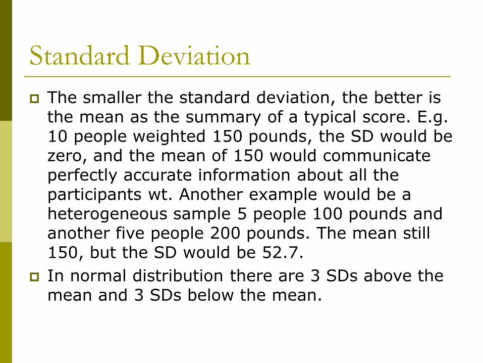
The smaller the standard deviation, the better is the mean as the summary of a typical score. E.g. 10 people weighted 150 pounds, the SD would be zero, and the mean of 150 would communicate perfectly accurate information about all the participants wt. Another example would be a heterogeneous sample 5 people 100 pounds and another five people 200 pounds. The mean still 150, but the SD would be 52.7.
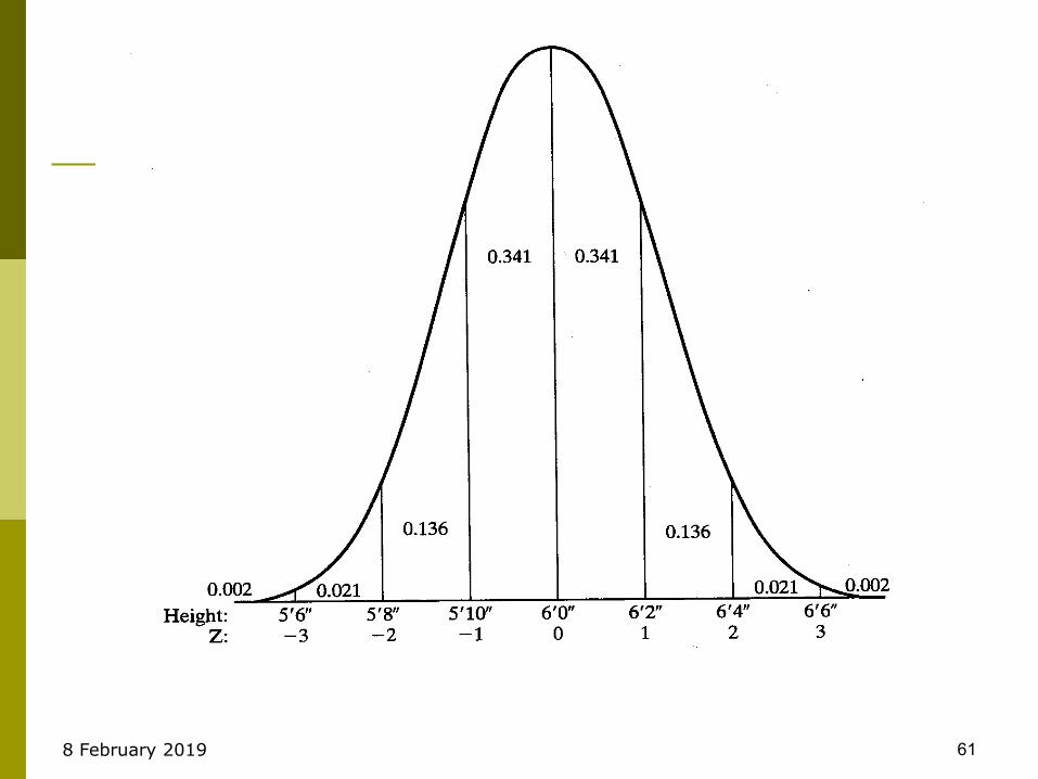
In normal distribution there are 3 SDs above the mean and 3 SDs below the mean.
46
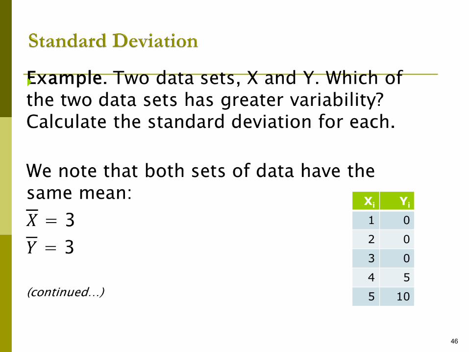
Xi Yi
1 0
2 0
3 0
4 5
5 10
47
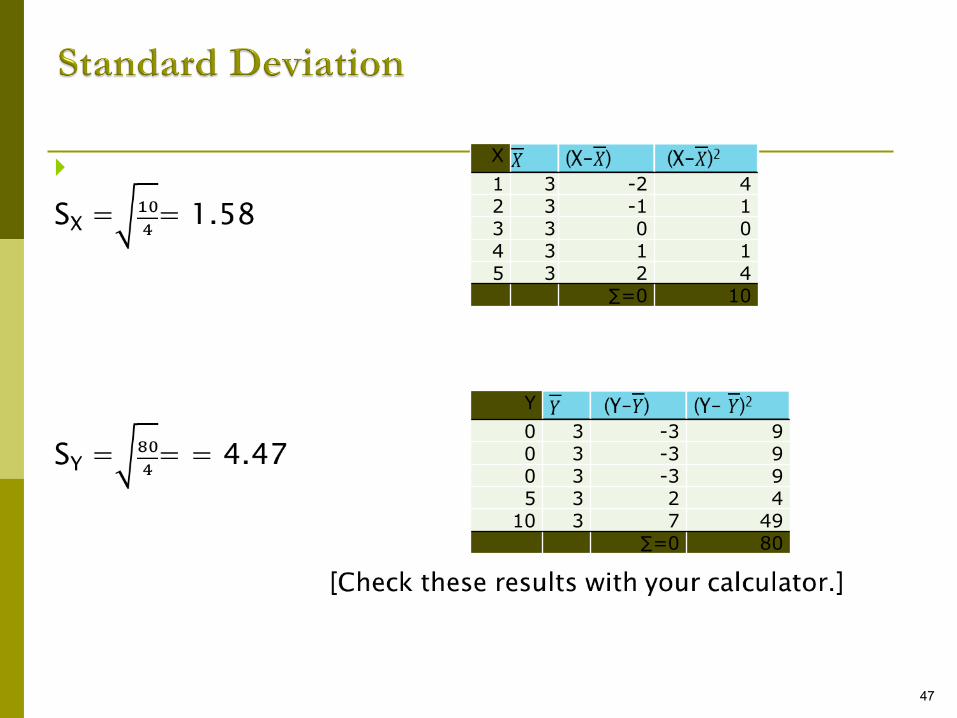
X
1 3 -2 42 3 -1 13 3 0 04 3 1 15 3 2 4
∑=0 10
Y
0 3 -3 90 3 -3 90 3 -3 95 3 2 4
10 3 7 49∑=0 80
48
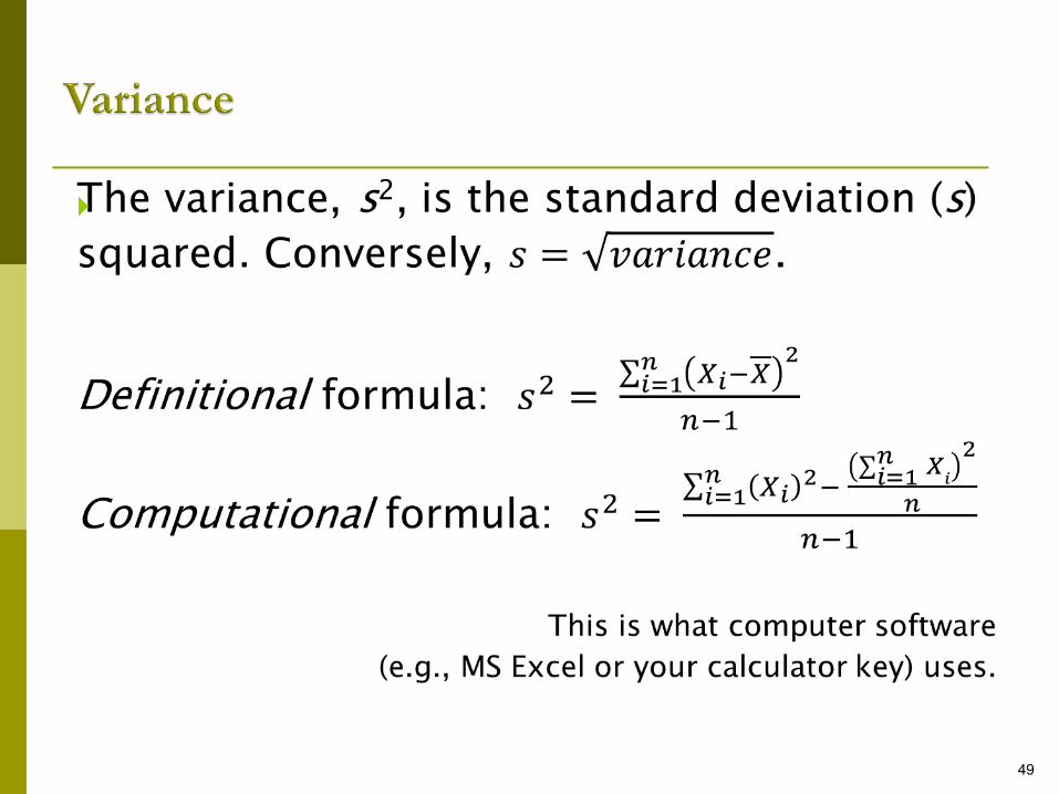
49
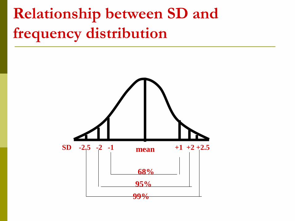
Relationship between SD and
frequency distribution
SD -2.5 -2 -1 +1 +2 +2.5mean
68%
95%
99%
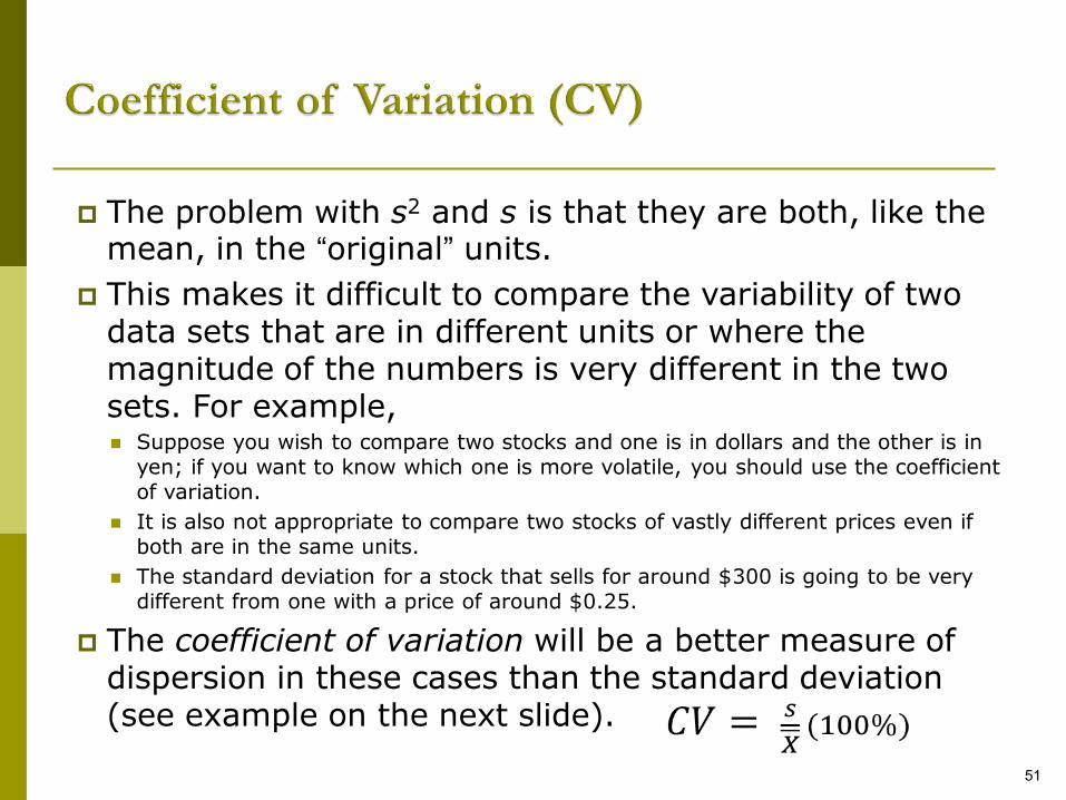
The problem with s2 and s is that they are both, like the mean, in the “original” units.
This makes it difficult to compare the variability of two data sets that are in different units or where the magnitude of the numbers is very different in the two sets. For example, Suppose you wish to compare two stocks and one is in dollars and the other is in
yen; if you want to know which one is more volatile, you should use the coefficient of variation.
It is also not appropriate to compare two stocks of vastly different prices even if both are in the same units.
The standard deviation for a stock that sells for around $300 is going to be very different from one with a price of around $0.25.
The coefficient of variation will be a better measure of dispersion in these cases than the standard deviation (see example on the next slide).
51
Descriptive Statistics I 52
Descriptive Statistics I 53
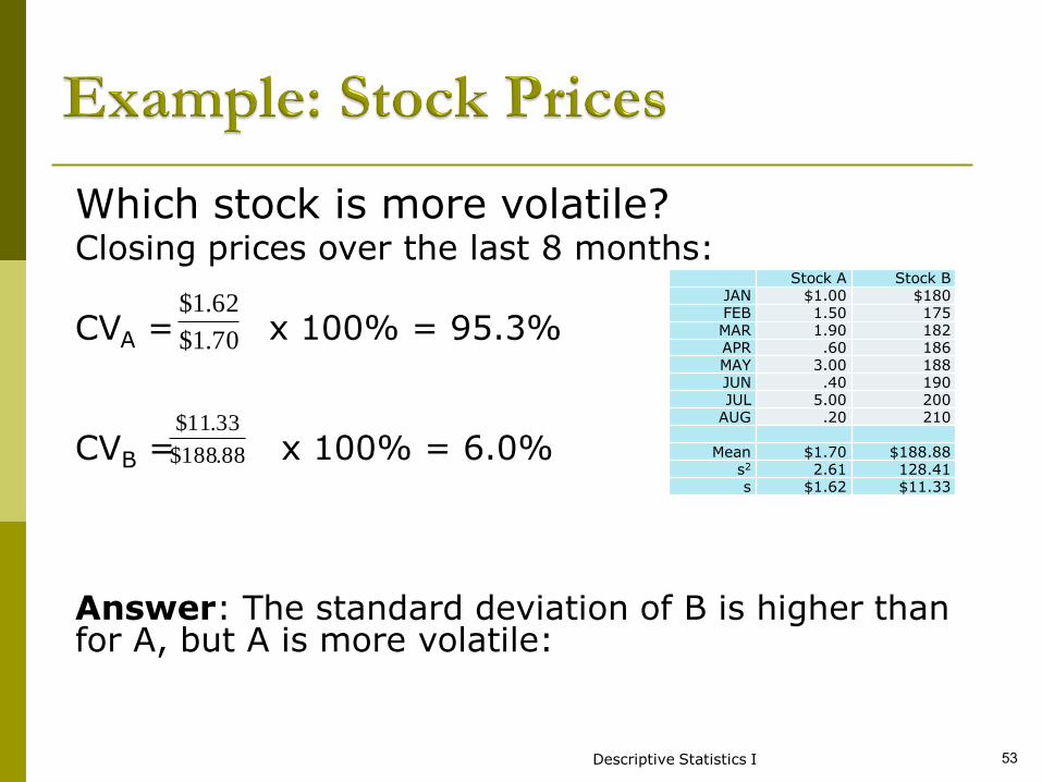
Which stock is more volatile?Closing prices over the last 8 months:
CVA = x 100% = 95.3%
CVB = x 100% = 6.0%
Answer: The standard deviation of B is higher than for A, but A is more volatile:
Stock A Stock BJAN $1.00 $180FEB 1.50 175MAR 1.90 182APR .60 186MAY 3.00 188JUN .40 190JUL 5.00 200
AUG .20 210
Mean $1.70 $188.88s2 2.61 128.41s $1.62 $11.33
70.1$
62.1$
88.188$
33.11$
54
IQR
The Interquartile range (IQR) is the score at the 75th percentile or 3rd quartile (Q3) minus the score at the 25th percentile or first quartile (Q1). Are the most used to define outliers.
It is not sensitive to extreme values.
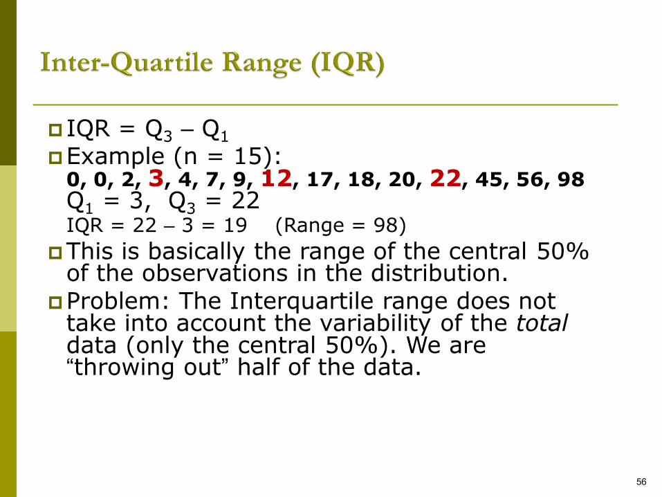
IQR = Q3 – Q1
Example (n = 15):0, 0, 2, 3, 4, 7, 9, 12, 17, 18, 20, 22, 45, 56, 98Q1 = 3, Q3 = 22IQR = 22 – 3 = 19 (Range = 98)
This is basically the range of the central 50% of the observations in the distribution.
Problem: The Interquartile range does not take into account the variability of the total data (only the central 50%). We are “throwing out” half of the data.
56
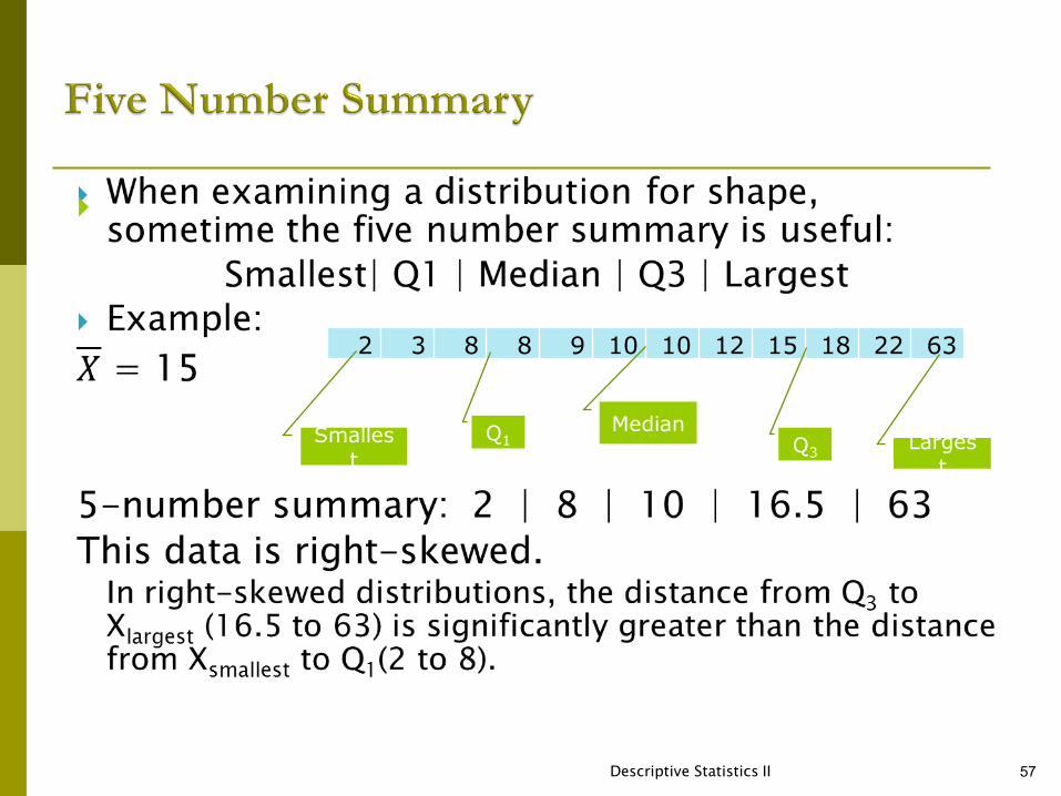
Descriptive Statistics II 57
2 3 8 8 9 10 10 12 15 18 22 63
Smallest
Largest
MedianQ1 Q3
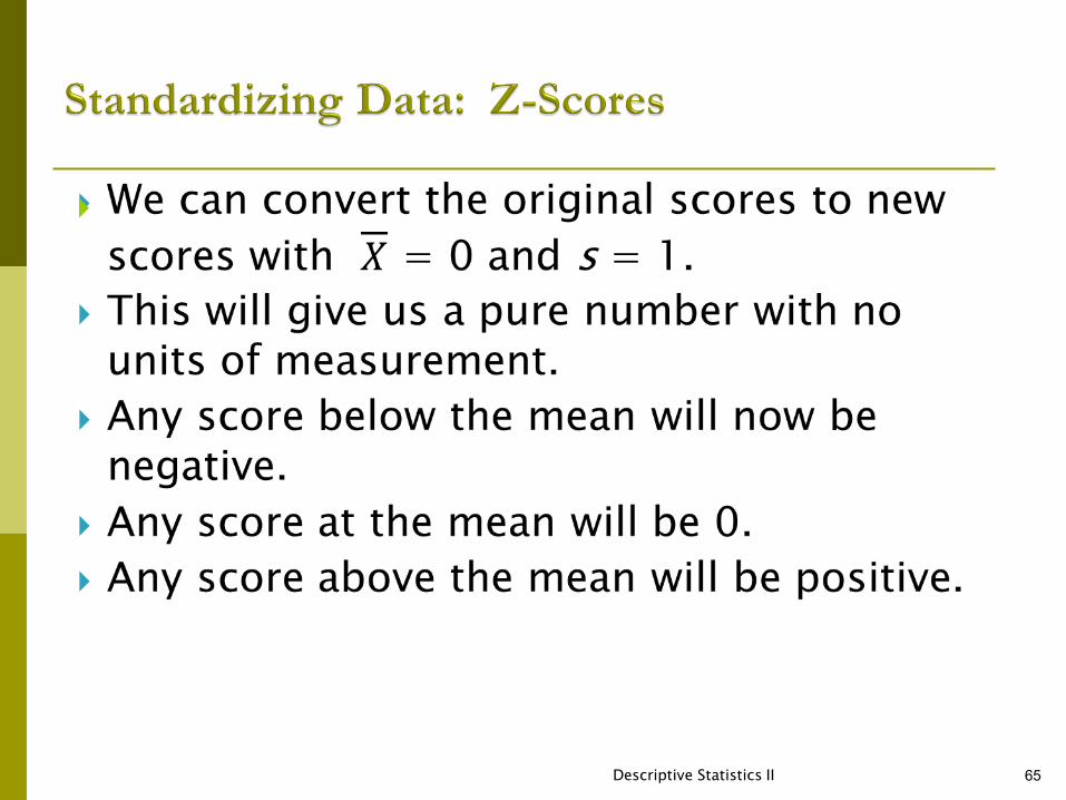
Standard Scores
There are scores that are expressed in terms of their relative distance from the mean. It provides information not only about rank but also distance between scores.
It often called Z-score.
Z Score
Is a standard score that indicates how many SDs from the mean a particular values lies.
Z = Score of value – mean of scores divided by standard deviation.
8 February 2019 60
Standard Normal Scores
How many standard deviations away from the mean are you?
Standard Score (Z) =
“Z” is normal with mean 0 and standard deviation of 1.
Observation – mean
Standard deviation
8 February 2019 61

8 February 2019 62
Standard Normal Scores
A standard score of:
Z = 1: The observation lies one SD above the mean
Z = 2: The observation is two SD above the mean
Z = -1: The observation lies 1 SD below the mean
Z = -2: The observation lies 2 SD below the mean
8 February 2019 63
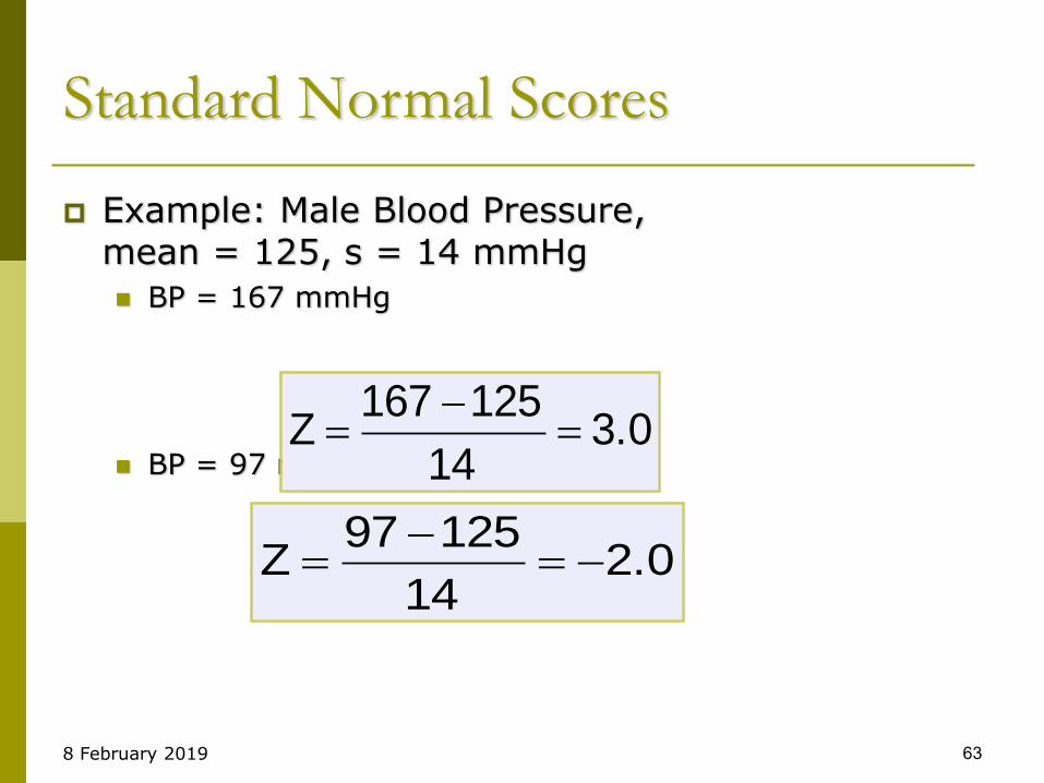
Standard Normal Scores
Example: Male Blood Pressure,mean = 125, s = 14 mmHg
BP = 167 mmHg
BP = 97 mmHg3.0
14
125167Z
2.014
12597Z
8 February 2019 64
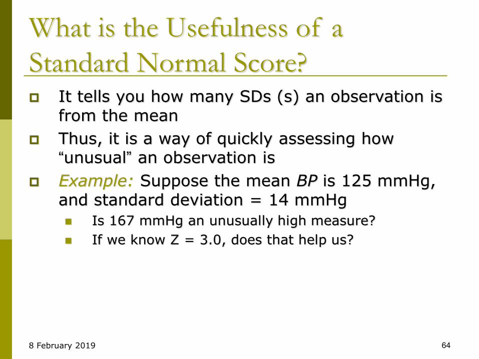
What is the Usefulness of a
Standard Normal Score? It tells you how many SDs (s) an observation is
from the mean
Thus, it is a way of quickly assessing how “unusual” an observation is
Example: Suppose the mean BP is 125 mmHg, and standard deviation = 14 mmHg
Is 167 mmHg an unusually high measure?
If we know Z = 3.0, does that help us?
Descriptive Statistics II 65
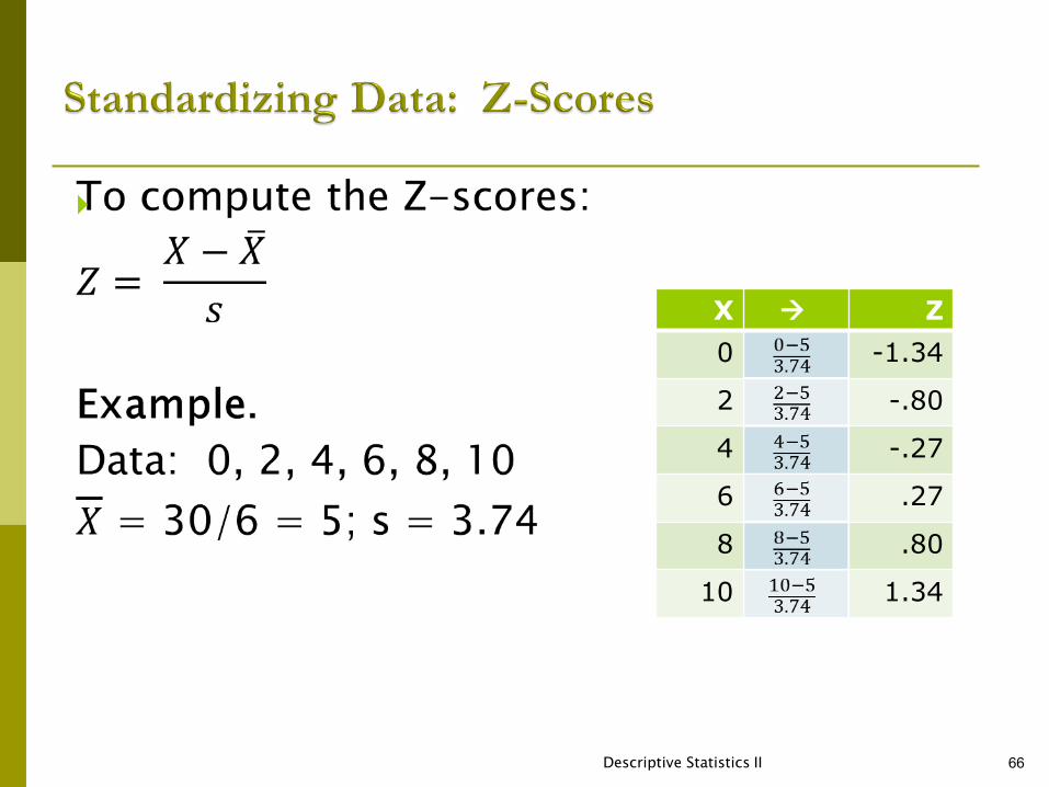
Descriptive Statistics II 66
X Z
0 -1.34
2 -.80
4 -.27
6 .27
8 .80
10 1.34
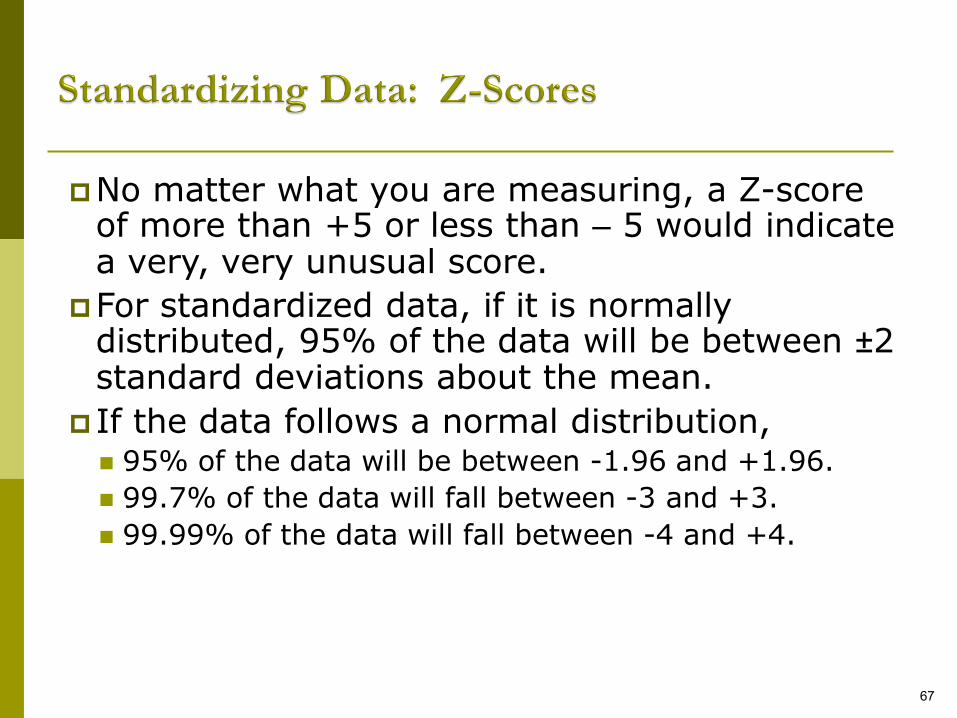
No matter what you are measuring, a Z-score of more than +5 or less than – 5 would indicate a very, very unusual score.
For standardized data, if it is normally distributed, 95% of the data will be between ±2 standard deviations about the mean.
If the data follows a normal distribution, 95% of the data will be between -1.96 and +1.96.
99.7% of the data will fall between -3 and +3.
99.99% of the data will fall between -4 and +4.
67
Major reasons for using Index
(descriptive statistics)
Understanding the data.
Evaluating outliers. Outliers are often identified in relation to the value of a distribution’s IQR. A mild outlier is a data value that lies between 1.5 and 3 times the IQR below Q1 or above Q3. Extreme outlier is a data value that is more that three times the IQR below Q1 or above Q3.
Describe the research sample.
Answering research questions.