Unit Test Generation usingMachine Learning

Laurence Saesl.saes@live.nl

August 23, 2018, 57 pages

Academic supervisor: dr. Ana OprescuHost organization: Info Support B.V. www.infosupport.comHost supervisor: Joop Snijder

Universiteit van AmsterdamFaculteit der Natuurwetenschappen, Wiskunde en InformaticaMaster Software Engineeringhttp://www.software-engineering-amsterdam.nl

Abstract

Test suite generators could help software engineers to ensure software quality by detecting softwarefaults. These generators can be applied to software projects that do not have an initial test suite, atest suite can be generated which is maintained and optimized by the developers. Testing helps tocheck if a program works and, also if it continues to work after changes. This helps to prevent softwarefrom failing and aids developers in applying changes and minimizing the possibility to introduce errorsin other (critical) parts of the software.

State-of-the-art test generators are still only able to capture a small portion of potential softwarefaults. The Search-Based Software Testing 2017 workshop compared four unit test generation tools.These generators were only capable of achieving an average mutation coverage below 51%, which islower than the score of the initial unit test suite written by software engineers.

We propose a test suite generator driven by neural networks, which has the potential to detectmutants that could only be detected by manually written unit tests. In this research, multiplenetworks, trained on open-source projects, are evaluated on their ability to generate test suites.The dataset contains the unit tests and the code it tests. The unit test method names are used tolink unit tests to methods under test.

With our linking mechanism, we were able to link 27.41% (36,301 out of 132,449) tests. Ourmachine learning model could generate parsable code in 86.69% (241/278) of the time. This highnumber of parsable code indicates that the neural network learned patterns between code and tests,which indicates that neural networks are applicable for test generation.

ACKNOWLEDGMENTS

This thesis is written for my software engineering master project at the University of Amsterdam.The research was conducted at Info Support B.V. in The Netherlands for the Business Unit Finance.

First, I would like to thank my supervisors Ana Oprescu of the University of Amsterdam and JoopSnijder of Info Support. Ana Oprescu was always available to give me feedback, guidance, and helpedme a lot with finding optimal solutions to resolve encountered problems. Joop Snijder gave me a lotof advice and background in machine learning. He helped me to understand how machine learningcould be applied in the project and what methods have great potential.

I would also like to thank Terry van Walen and Clemens Grelck for their help and support duringthis project. The brainstorm sessions with Terry were very helpful and gave a lot of new insights insolutions to the encountered problem. I am grateful for Clemens help too in order to prepare me forthe conferences. My presentation skills have improved a lot and I really enjoyed the opportunity

Finally, I would like the thank the University of Amsterdam and Info Support B.V. for all theirhelp and funding so that I could present at CompSys 2018 in Leusen, Netherlands, and Sattose 2018in Athens, Greece. This was a great learning experience, and I am very grateful to have had theseopportunities.

i

Contents

Abstract

ACKNOWLEDGMENTS i

1 Introduction 11.1 Types of testing . . . . . . . . . . . . . . . . . . . . . . . . . . . . . . . . . . . . . . . . 11.2 Neural networks . . . . . . . . . . . . . . . . . . . . . . . . . . . . . . . . . . . . . . . 21.3 Research questions . . . . . . . . . . . . . . . . . . . . . . . . . . . . . . . . . . . . . . 31.4 Contribution . . . . . . . . . . . . . . . . . . . . . . . . . . . . . . . . . . . . . . . . . 31.5 Outline . . . . . . . . . . . . . . . . . . . . . . . . . . . . . . . . . . . . . . . . . . . . 3

2 Background 42.1 Test generation . . . . . . . . . . . . . . . . . . . . . . . . . . . . . . . . . . . . . . . . 4

2.1.1 Test oracles . . . . . . . . . . . . . . . . . . . . . . . . . . . . . . . . . . . . . . 42.2 Code analysis . . . . . . . . . . . . . . . . . . . . . . . . . . . . . . . . . . . . . . . . . 42.3 Machine learning techniques . . . . . . . . . . . . . . . . . . . . . . . . . . . . . . . . . 5

3 A Machine Learning-based Test Suite Generator 63.1 Data collection . . . . . . . . . . . . . . . . . . . . . . . . . . . . . . . . . . . . . . . . 6

3.1.1 Selecting a test framework . . . . . . . . . . . . . . . . . . . . . . . . . . . . . . 63.1.2 Testable projects . . . . . . . . . . . . . . . . . . . . . . . . . . . . . . . . . . . 63.1.3 Number of training examples . . . . . . . . . . . . . . . . . . . . . . . . . . . . 7

3.2 Linking code to test . . . . . . . . . . . . . . . . . . . . . . . . . . . . . . . . . . . . . 73.2.1 Linking algorithm . . . . . . . . . . . . . . . . . . . . . . . . . . . . . . . . . . 73.2.2 Linking methods . . . . . . . . . . . . . . . . . . . . . . . . . . . . . . . . . . . 8

3.3 Machine learning datasets . . . . . . . . . . . . . . . . . . . . . . . . . . . . . . . . . . 93.3.1 Training set . . . . . . . . . . . . . . . . . . . . . . . . . . . . . . . . . . . . . . 93.3.2 Validation set . . . . . . . . . . . . . . . . . . . . . . . . . . . . . . . . . . . . . 93.3.3 Test set . . . . . . . . . . . . . . . . . . . . . . . . . . . . . . . . . . . . . . . . 9

4 Evaluation Setup 104.1 Evaluation . . . . . . . . . . . . . . . . . . . . . . . . . . . . . . . . . . . . . . . . . . . 10

4.1.1 Metrics . . . . . . . . . . . . . . . . . . . . . . . . . . . . . . . . . . . . . . . . 104.1.2 Measurement . . . . . . . . . . . . . . . . . . . . . . . . . . . . . . . . . . . . . 114.1.3 Comparing machine learning models . . . . . . . . . . . . . . . . . . . . . . . . 11

4.2 Baseline . . . . . . . . . . . . . . . . . . . . . . . . . . . . . . . . . . . . . . . . . . . . 11

5 Experimental Setup 125.1 Data collection . . . . . . . . . . . . . . . . . . . . . . . . . . . . . . . . . . . . . . . . 12

5.1.1 Additional project criteria . . . . . . . . . . . . . . . . . . . . . . . . . . . . . . 125.1.2 Collecting projects . . . . . . . . . . . . . . . . . . . . . . . . . . . . . . . . . . 125.1.3 Training data . . . . . . . . . . . . . . . . . . . . . . . . . . . . . . . . . . . . . 13

5.2 Extraction training examples . . . . . . . . . . . . . . . . . . . . . . . . . . . . . . . . 135.2.1 Building the queue . . . . . . . . . . . . . . . . . . . . . . . . . . . . . . . . . . 13

5.3 Training machine learning models . . . . . . . . . . . . . . . . . . . . . . . . . . . . . . 14

ii

5.3.1 Tokenized view . . . . . . . . . . . . . . . . . . . . . . . . . . . . . . . . . . . . 145.3.2 Compression . . . . . . . . . . . . . . . . . . . . . . . . . . . . . . . . . . . . . 145.3.3 BPE . . . . . . . . . . . . . . . . . . . . . . . . . . . . . . . . . . . . . . . . . . 155.3.4 Abstract syntax tree . . . . . . . . . . . . . . . . . . . . . . . . . . . . . . . . . 15

5.4 Experiments . . . . . . . . . . . . . . . . . . . . . . . . . . . . . . . . . . . . . . . . . . 165.4.1 The ideal subset of training examples and basic network configuration . . . . . 165.4.2 SBT data representation . . . . . . . . . . . . . . . . . . . . . . . . . . . . . . . 175.4.3 BPE data representation . . . . . . . . . . . . . . . . . . . . . . . . . . . . . . . 175.4.4 Compression (with various levels) data representation . . . . . . . . . . . . . . 175.4.5 Different network configurations . . . . . . . . . . . . . . . . . . . . . . . . . . 175.4.6 Compression timing . . . . . . . . . . . . . . . . . . . . . . . . . . . . . . . . . 175.4.7 Compression accuracy . . . . . . . . . . . . . . . . . . . . . . . . . . . . . . . . 185.4.8 Finding differences between experiments . . . . . . . . . . . . . . . . . . . . . . 18

6 Results 206.1 Linking experiments . . . . . . . . . . . . . . . . . . . . . . . . . . . . . . . . . . . . . 20

6.1.1 Removing redundant tests . . . . . . . . . . . . . . . . . . . . . . . . . . . . . . 206.1.2 Unit test support . . . . . . . . . . . . . . . . . . . . . . . . . . . . . . . . . . . 206.1.3 Linking capability . . . . . . . . . . . . . . . . . . . . . . . . . . . . . . . . . . 216.1.4 Total links . . . . . . . . . . . . . . . . . . . . . . . . . . . . . . . . . . . . . . 226.1.5 Linking difference . . . . . . . . . . . . . . . . . . . . . . . . . . . . . . . . . . 22

6.2 Experiments for RQ1 . . . . . . . . . . . . . . . . . . . . . . . . . . . . . . . . . . . . 236.2.1 Naive approach . . . . . . . . . . . . . . . . . . . . . . . . . . . . . . . . . . . . 246.2.2 Training data simplification . . . . . . . . . . . . . . . . . . . . . . . . . . . . . 266.2.3 Training data simplification follow-up . . . . . . . . . . . . . . . . . . . . . . . 286.2.4 Combination of simplifications . . . . . . . . . . . . . . . . . . . . . . . . . . . 306.2.5 Different data representations . . . . . . . . . . . . . . . . . . . . . . . . . . . . 316.2.6 Different network configurations . . . . . . . . . . . . . . . . . . . . . . . . . . 336.2.7 Generated predictions . . . . . . . . . . . . . . . . . . . . . . . . . . . . . . . . 356.2.8 Experiment analysis . . . . . . . . . . . . . . . . . . . . . . . . . . . . . . . . . 36

6.3 Experiments for RQ2 . . . . . . . . . . . . . . . . . . . . . . . . . . . . . . . . . . . . 396.3.1 Compression timing . . . . . . . . . . . . . . . . . . . . . . . . . . . . . . . . . 396.3.2 Compression accuracy . . . . . . . . . . . . . . . . . . . . . . . . . . . . . . . . 40

6.4 Applying SBT in the experiments . . . . . . . . . . . . . . . . . . . . . . . . . . . . . . 426.4.1 Output length . . . . . . . . . . . . . . . . . . . . . . . . . . . . . . . . . . . . 426.4.2 Training . . . . . . . . . . . . . . . . . . . . . . . . . . . . . . . . . . . . . . . . 436.4.3 First steps to a solution . . . . . . . . . . . . . . . . . . . . . . . . . . . . . . . 43

7 Discussion 447.1 Summary of the results . . . . . . . . . . . . . . . . . . . . . . . . . . . . . . . . . . . 447.2 RQ1: What neural network solutions can be applied to generate test suites in order to

achieve a higher test suite effectiveness for software projects? . . . . . . . . . . . . . . 447.2.1 The parsable code metric . . . . . . . . . . . . . . . . . . . . . . . . . . . . . . 447.2.2 Training on a limited sequence size . . . . . . . . . . . . . . . . . . . . . . . . . 457.2.3 Using training examples with common subsequences . . . . . . . . . . . . . . . 457.2.4 BPE . . . . . . . . . . . . . . . . . . . . . . . . . . . . . . . . . . . . . . . . . . 457.2.5 Network configuration of related research . . . . . . . . . . . . . . . . . . . . . 457.2.6 SBT . . . . . . . . . . . . . . . . . . . . . . . . . . . . . . . . . . . . . . . . . . 457.2.7 Comparing our models . . . . . . . . . . . . . . . . . . . . . . . . . . . . . . . . 46

7.3 RQ2: What is the impact of input and output sequence compression on the trainingtime and accuracy? . . . . . . . . . . . . . . . . . . . . . . . . . . . . . . . . . . . . . . 467.3.1 Training time reduction . . . . . . . . . . . . . . . . . . . . . . . . . . . . . . . 467.3.2 Increasing loss . . . . . . . . . . . . . . . . . . . . . . . . . . . . . . . . . . . . 46

7.4 Limitations . . . . . . . . . . . . . . . . . . . . . . . . . . . . . . . . . . . . . . . . . . 467.4.1 The used mutation testing tool . . . . . . . . . . . . . . . . . . . . . . . . . . . 47

iii

7.4.2 JUnit version . . . . . . . . . . . . . . . . . . . . . . . . . . . . . . . . . . . . . 477.4.3 More links for AST analysis depends on data . . . . . . . . . . . . . . . . . . . 477.4.4 False positive links . . . . . . . . . . . . . . . . . . . . . . . . . . . . . . . . . . 47

7.5 The dataset has an impact on the test generators quality . . . . . . . . . . . . . . . . 477.5.1 Generation calls to non-existing methods . . . . . . . . . . . . . . . . . . . . . 477.5.2 Testing a complete method . . . . . . . . . . . . . . . . . . . . . . . . . . . . . 477.5.3 The machine learning model is unaware of implementations . . . . . . . . . . . 487.5.4 Too less data for statistical proving our models . . . . . . . . . . . . . . . . . . 487.5.5 Replacing manual testing . . . . . . . . . . . . . . . . . . . . . . . . . . . . . . 48

8 Related work 49

9 Conclusion 50

10 Future work 5110.1 SBT and BPE . . . . . . . . . . . . . . . . . . . . . . . . . . . . . . . . . . . . . . . . 5110.2 Common subsequences . . . . . . . . . . . . . . . . . . . . . . . . . . . . . . . . . . . . 51

10.2.1 Filtering code complexity with other algorithms . . . . . . . . . . . . . . . . . 5110.3 Promising areas . . . . . . . . . . . . . . . . . . . . . . . . . . . . . . . . . . . . . . . . 51

10.3.1 Reducing the time required to train models . . . . . . . . . . . . . . . . . . . . 5110.3.2 Optimized machine learning algorithm . . . . . . . . . . . . . . . . . . . . . . . 52

Bibliography 53

A Data and developed software 56

iv

List of Figures

1.1 Visualization of a neural network . . . . . . . . . . . . . . . . . . . . . . . . . . . . . . . . 2

3.1 Possible development flow for the test suite generator . . . . . . . . . . . . . . . . . . . . 6

5.1 Example of tokenized view . . . . . . . . . . . . . . . . . . . . . . . . . . . . . . . . . . . 145.2 Example of compression view . . . . . . . . . . . . . . . . . . . . . . . . . . . . . . . . . . 155.3 Example of BPE view . . . . . . . . . . . . . . . . . . . . . . . . . . . . . . . . . . . . . . 155.4 Example of AST view . . . . . . . . . . . . . . . . . . . . . . . . . . . . . . . . . . . . . . 16

6.1 Supported unit test by bytecode analysis and AST analysis . . . . . . . . . . . . . . . . . 216.2 Unit test links made on tests supported by bytecode analysis and AST analysis . . . . . . 216.3 Total link with AST analysis and bytecode analysis . . . . . . . . . . . . . . . . . . . . . 226.4 Roadmap of all experiments . . . . . . . . . . . . . . . . . . . . . . . . . . . . . . . . . . 246.5 Experiments within the native approach group . . . . . . . . . . . . . . . . . . . . . . . . 266.6 Experiments within the training data simplification group . . . . . . . . . . . . . . . . . . 286.7 Experiments in optimizing sequence length . . . . . . . . . . . . . . . . . . . . . . . . . . 306.8 Experiments in combination of optimizations . . . . . . . . . . . . . . . . . . . . . . . . . 316.9 Maximum sequence length differences with various levels of compression . . . . . . . . . . 326.10 Experiments with different data representations . . . . . . . . . . . . . . . . . . . . . . . 336.11 Experiments in different network configurations . . . . . . . . . . . . . . . . . . . . . . . 356.12 All experiment results . . . . . . . . . . . . . . . . . . . . . . . . . . . . . . . . . . . . . . 376.13 Compression timing scatter plot . . . . . . . . . . . . . . . . . . . . . . . . . . . . . . . . 396.14 Loss for every 100th epoch . . . . . . . . . . . . . . . . . . . . . . . . . . . . . . . . . . . 41

v

List of Tables

4.1 Mutation coverage by project . . . . . . . . . . . . . . . . . . . . . . . . . . . . . . . . . . 11

6.1 Details on naive approach experiment . . . . . . . . . . . . . . . . . . . . . . . . . . . . . 256.2 Details on experiment with less complex training data . . . . . . . . . . . . . . . . . . . . 266.3 Details on experiment with common subsequences . . . . . . . . . . . . . . . . . . . . . . 276.4 Details on experiment with maximum sequence size 100 . . . . . . . . . . . . . . . . . . . 276.5 Details on experiment with maximum sequence size 200 and limited number of training

examples . . . . . . . . . . . . . . . . . . . . . . . . . . . . . . . . . . . . . . . . . . . . . 286.6 Details on experiment with maximum sequence size 200 and more training examples . . . 296.7 Details on experiment with maximum sequence size 300 and limited number of training

examples . . . . . . . . . . . . . . . . . . . . . . . . . . . . . . . . . . . . . . . . . . . . . 296.8 Details on experiment with maximum sequence size 100 and common subsequences . . . 306.9 Details on experiment with maximum sequence size 100 and no concrete classes and no

default methods . . . . . . . . . . . . . . . . . . . . . . . . . . . . . . . . . . . . . . . . . 316.10 Details on experiment with maximum sequence size 100, common subsequences, and com-

pression . . . . . . . . . . . . . . . . . . . . . . . . . . . . . . . . . . . . . . . . . . . . . . 326.11 Details on experiment with maximum sequence size 100, common subsequences, and BPE 336.12 Overview of all network experiments . . . . . . . . . . . . . . . . . . . . . . . . . . . . . . 346.13 Details on experiment with maximum sequence size 100, common subsequences, and dif-

ferent network configurations . . . . . . . . . . . . . . . . . . . . . . . . . . . . . . . . . . 346.14 Parsable code score for the most important experiments with different seeds . . . . . . . 376.15 ANOVA experiment results . . . . . . . . . . . . . . . . . . . . . . . . . . . . . . . . . . . 386.16 Difference between experiments . . . . . . . . . . . . . . . . . . . . . . . . . . . . . . . . . 386.17 Directional t-test of significantly different experiments . . . . . . . . . . . . . . . . . . . . 396.18 ANOVA on compression timing . . . . . . . . . . . . . . . . . . . . . . . . . . . . . . . . . 406.19 Difference in compression timing . . . . . . . . . . . . . . . . . . . . . . . . . . . . . . . . 406.20 Directional t-test on compression timing . . . . . . . . . . . . . . . . . . . . . . . . . . . . 406.21 ANOVA experiment for compression loss . . . . . . . . . . . . . . . . . . . . . . . . . . . 416.22 Difference in loss groups . . . . . . . . . . . . . . . . . . . . . . . . . . . . . . . . . . . . . 426.23 Directional t-test on compression loss . . . . . . . . . . . . . . . . . . . . . . . . . . . . . 426.24 SBT compression effect . . . . . . . . . . . . . . . . . . . . . . . . . . . . . . . . . . . . . 43

8.1 Machine learning projects that translate to or from code . . . . . . . . . . . . . . . . . . 49

A.1 Overview of the GitHub repository . . . . . . . . . . . . . . . . . . . . . . . . . . . . . . . 56A.2 Overview of the Stack directory . . . . . . . . . . . . . . . . . . . . . . . . . . . . . . . . 57

vi

Chapter 1

Introduction

Test suites are used to ensure software quality when a program’s code base evolves. The capabilityof producing the desired effect (effectiveness) of a test suite is often measured as the ability to un-cover faults in a program [ZM15]. Although intensively researched [AHF+17, KC17, CDE+08, FZ12,REP+11], state-of-the-art test suite generators lack test coverage that could be achieved with manualtesting. Almasi et al. [AHF+17] explained a category of faults that are not detectable by these testsuite generators. These faults are usually surrounded by complex conditions and statements for whichcomplex objects have to be constructed and populated with specific values.

The Search-Based Software Testing (SBST) Workshop of 2017 had a competition of Java unit testgenerators. In the competition, test suite effectiveness of test suite generators and manually writtentest suites were evaluated. The effectiveness of the test suites are measured by their ability to findfaults and is measured with the mutation score metric. The ability to find faults can be measured withmutation score because mutations are a valid substitute for software faults [JJI+14]. The mutationscore of a test suite represents the test suite’s ability to detect syntactic variations of the source code(mutants), and is computed using a mutation testing framework. In the workshop, manually writtentest suites score on average 53.8% mutation coverage, while the highest score obtained by a generatedtest suite is 50.8% [FRCA17].

However, it is impossible to conclude that all possible mutants are detected even when all generatedmutants are covered since the list of possible mutations is infinite. It is infinite because some methodscan have an infinite amount of output values, and mutants can be introduced that only change oneof these output values.

We need to leverage the ability to automatically test many different execution paths and the capa-bility to learn how to test complex situations of generated and manually written test suites. Therefore,we propose a test suite generator that uses machine learning techniques.

A neural network is a machine learning algorithm, that can learn complex tasks without beingprogrammed with rules. The network learns from examples and captures the logic that is inside.Thus, new rules can be taught to the neural network by just showing examples of how the translationis done.

Our solution uses neural networks and combines manual and automated test suites by learningpatterns between tests and code to generate test suites with higher effectiveness.

1.1 Types of testing

There are two software testing methods, i) black box testing [Ost02a] and ii) white box testing[Ost02b]. With black box testing, the project’s source code is not used to create tests. Only thespecification of the software is used [LKT09]. White box testing is a method that uses the sourcecode to create tests. The source code is evaluated, and its behavior is captured [LKT09]. White boxtesting focuses more on the inner working of the software, while black box testing focuses more onspecifications [ND12]. Black box testing is more efficient with testing of large code blocks as only thespecification has to be evaluated, while white box testing is more efficient in testing hidden logic.

1

Our unit test generator can be categorized as white box testing since we use the source code togenerate tests.

1.2 Neural networks

Neural networks are inspired by how our brains work [Maa97]. Our brain uses an interconnectednetwork of neurons to process everything that we observe. A neuron is a cell that receives inputfrom other neurons. An observation is sent to the network as the input signal. Each neuron in thenetwork sends a signal to the next cells in the network based on the signals that it received. With thisapproach, the input translates to particular values at the output of the network. Humans performactions based on this output. This mechanism is similar to the concept of how a neural networkworks.

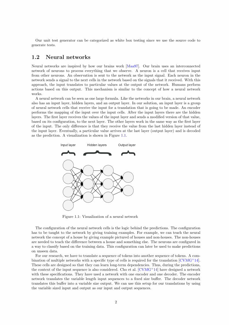
A neural network can be seen as one large formula. Like the networks in our brain, a neural networkalso has an input layer, hidden layers, and an output layer. In our solution, an input layer is a groupof neural network cells that receive the input for a translation that is going to be made. An encoderperforms the mapping of the input over the input cells. After the input layers there are the hiddenlayers. The first layer receives the values of the input layer and sends a modified version of that value,based on its configuration, to the next layer. The other layers work in the same way as the first layerof the input. The only difference is that they receive the value from the last hidden layer instead ofthe input layer. Eventually, a particular value arrives at the last layer (output layer) and is decodedas the prediction. A visualization is shown in Figure 1.1.

Figure 1.1: Visualization of a neural network

The configuration of the neural network cells is the logic behind the predictions. The configurationhas to be taught to the network by giving training examples. For example, we can teach the neuralnetwork the concept of a house by giving example pictured of houses and non-houses. The non-housesare needed to teach the difference between a house and something else. The neurons are configured ina way to classify based on the training data. This configuration can later be used to make predictionson unseen data.

For our research, we have to translate a sequence of tokens into another sequence of tokens. A com-bination of multiple networks with a specific type of cells is required for the translation [CVMG+14].These cells are designed so that they can learn long-term dependencies. Thus, during the predictions,the context of the input sequence is also considered. Cho et al. [CVMG+14] have designed a networkwith these specifications. They have used a network with one encoder and one decoder. The encodernetwork translates the variable length input sequences to a fixed size buffer. The decoder networktranslates this buffer into a variable size output. We can use this setup for our translations by usingthe variable sized input and output as our input and output sequences.

2

1.3 Research questions

Our research goal is to study machine learning approaches to generate test suites with high ef-fectiveness: learn how code and tests are linked and apply this logic on the project’s code base.Although neural networks are widely used for translation problems [SVL14], training them is oftentime-consuming. Therefore, we also research heuristics to alleviate this issue. This is translated intothe following research questions:

RQ1 What neural network solutions can be applied to generate test suites in order to achieve a highertest suite effectiveness for software projects?

RQ2 What is the impact of input and output sequence compression on the training time and accuracy?

1.4 Contribution

In this work, we contribute an algorithm to link unit tests to the method under test, a training setfor translating code to tests with more than 52,000 training examples, software to convert code todifferent representations and also support the translation back, and a neural network configurationwith the ability to learn patterns between code and tests. Finally, we also contribute a pipeline thattakes as input GitHub repositories and has as output a machine learning model that can be used topredict tests. As far as we know, we are the first to perform experiments in this area. Therefore, thelinking algorithm and the neural network configuration can be used as a baseline for future research.The dataset can also be used on varies other types of machine learning algorithms for the developmentof a test generator.

1.5 Outline

We address the background of test generation, code analysis and machine learning in Chapter 2. InChapter 3, we discuss how a test generator could be designed in general that uses machine learning.In Chapter 4, we list projects that can be used for evaluation baseline, and we introduce metrics tomeasure the progress of developing the test suite generator and how well it performed compared toother generators on a baseline. How we develop our test generator can be found in Chapter 5. Ourresults are presented in Chapter 6 and discussed in Chapter 7. Related work is listed in Chapter 8.We conclude our work in Chapter 9. Finally, an overview of related work to this thesis can found inChapter 10.

3

Chapter 2

Background

Multiple approaches address the challenge of achieving a high test suite effectiveness. Tests could begenerated based on the project’s source code by analyzing all possible execution paths. An alternativeis using test oracles, which can be trained to distinguish between correct and incorrect method output.Additionally, many code analysis techniques can be used to gather training examples and manymachine learning algorithms can be used to translate from and/or to code.

2.1 Test generation

Common methods for code-based test generation are random testing [AHF+17], search-based test-ing [FRCA17, AHF+17], and symbolic testing [CDE+08]. Almasi et al. benchmarked random testingand search-based testing on the closed source project LifeCalc [AHF+17] and found that search-basedtesting had at most 56.40% effectiveness, while random testing achieved at most 38%. They didnot analyze symbolic testing because there was no symbolic testing tool available that supported theanalyzed project’s language. Cadar et al. [CDE+08] applied symbolic testing on the HiStar kernelachieving 76.4% test suite effectiveness compared to 48.0% with random testing.

2.1.1 Test oracles

A test oracle is a mechanism that can be used to determine whether a method output is correct orincorrect. Testing is performed by executing the method under test with random data and evaluatingthe output with the test oracle.

Fraser et al. [FZ12] analyzed an oracle generator that generated assertions based upon mutationscore. For Joda-time, the oracle generator covered 82.95% of the mutants compared to 74.26% for themanual test suite. For Commons-Math, the oracle generator covered 58.61% of the mutants comparedto 41.25% for the manual test suite. Their test oracle generator employs machine learning to create thetest oracles. Each test oracle captures method behavior for a single method in the software programby training on the method with random input. Contrary to this approach, our proposed methodgenerates code while this method predicts the output of methods.

2.2 Code analysis

Multiple methods can be used to analyze code. Two possibilities are the analysis of i) bytecode or ii)the program’s source code. The biggest difference between bytecode analysis and source code analysisis that bytecode is closer to the instructions that form the real program and has the advantage ofmore available concrete type information. For this language, it is easier to construct a call graph,which can be used to determine the concrete class of certain method calls.

With the analysis of bytecode, the output of the Java compiler is analyzed and could be performedby using libraries. For instance, the T.J. Watson Libraries for Analysis (WALA) 1. The library will

1http://wala.sourceforge.net

4

generate the call graph and provides functionality that can be applied on the graph. With the analysisof source code, the source code in the representation of an abstract syntax tree (AST) is analyzed. ForAST analysis, JavaParser 2 can be used to construct an AST, and the library provides functionalityto perform operations on the tree.

2.3 Machine learning techniques

Multiple neural network solutions could translate sequences (translating an input sequence to atranslated sequence). For our research, we expect that sequence-to-sequence (seq2seq) neural net-works based on recurrent neural networks (RNNs) or convolutional neural networks (CNNs) are mostpromising. The version that uses RNNs can be configured to contain long short-term memory (LSTM)nodes [SVL14, SSN12] or gated recurrent unit (GRU) nodes [YKYS17a] and can be configured withan attention mechanism so it can make predictions on long sequences [BCB14]. Bahdanau [BCB14]evaluated the attention mechanism. They tested sequence length until a length of 60 tokens and usedbilingual evaluation understudy (BLEU) score as metric. The BLEU score is used to calculate thequality of translations. The higher the score, the better. The quality of the predictions was the samefor using both attention or no attention mechanism until a length of 20 tokens. The quality droppedfrom approximately 27 BLEU to approximately 8 BLEU when using no attention mechanism, anddropped from approximately 27 BLEU to approximately 26 BLEU when using an attention mecha-nism. Chung et al. [CGCB14] made a comparison between LSTM nodes and GRU nodes to predictthe next time step in songs. They found that the quality of prediction of both LSTM and GRU arecomparable. GRU outperforms except on one dataset by Ubisoft. However, they stated that theprediction quality of both could not be clearly distinguished. These networks could perform well totranslate code to unit tests because they can make predictions on long sequences.

An alternative to RNNs, are CNNs. Recent research shows that CNNs can also be applied tomake predictions based on source code [APS16]. In addition, Gehring et al. [GAG+17] were able totrain CNN models up to 21.3 times faster compared to RNN models. However, in other research,GRU outperforms CNN with handling long sequences correctly [YKYS17b]. We also look into CNNsbecause in our case it could make better predictions, especially because they are faster to train whatenables us to use larger networks.

There are also techniques in research that could be used to prepare the training data in order tooptimize the training process. Hu et al. [HWLJ18] used a structure-based traversal (SBT) in order tocapture code structure in a textual representation, Ling et al. [LGH+16] used compression to reducesequence lengths, and Sennrich et al. used byte pair encoding (BPE) [SHB15] to support betterpredictions on words that are written differently but have the same meaning.

In conclusion, to answer RQ1, we evaluate both CNNs and RNNs, as both tools look promising.We apply SBT, code compression, and BPE to find out if these techniques improve the results whentranslating methods into unit tests.

2https://javaparser.org/

5

Chapter 3

A Machine Learning-based TestSuite Generator

Our solution focuses on generating test suites for Java projects that have no test suite at all. Thesolution requires the project’s method bodies and the name of the classes to which they belong. Thetest generator sends the method bodies in a textual representation to the neural network to transformthem into test method bodies. The test generator places these generated methods in test classes.The collection of all the new test classes is the new test suite. This test suite can be used to test theproject’s source code on faults.

In an ideal situation, a model is already trained. When this is not the case, then additional actionsare required. Training projects are selected to train the network to generate usable tests. For instance,all training projects should use the same unit test framework. A unit test linking algorithm is usedto extract training examples from these projects. The found methods and the unit test method aregiven as training examples to the neural network. The model can then be created by training a neuralnetwork on these training examples. A detailed example of a possible flow can be found in Figure 3.1.

Figure 3.1: Possible development flow for the test suite generator

3.1 Data collection

We set some criteria to ensure that we have useful training examples. In addition, we need a thresholdon the number of training examples that should be gathered, because a large amount might not benecessary and is more time-consuming, while too few will affect the accuracy of the model.

3.1.1 Selecting a test framework

The test generator should not generate tests that use different frameworks since each framework worksdifferently. Therefore, it is important to select projects using only one testing framework. In 2018,Oracle reviewed what Java frameworks are the most popular [Poi]. They concluded that the unit testframework Junit is the most used. We selected Junit as test framework based on its popularity. Weexpect that we require a large amount of test data to train the neural network model.

3.1.2 Testable projects

Unit tests that fail are unusable for our research. Our test generator should generate unit teststhat test a piece of code. When a test fails, it fails due to an issue. It is not sure if the issue is amismatch between the method’s behavior and the behavior captured in the test. These tests should

6

not be included because a mismatch in behavior could teach the neural network patterns that preventtesting correctly. So, the tests have to be analyzed in order to filter out tests that fail. For thefiltering, we execute the unit test from the projects, analyze the reports, and extract all the tests thatsucceed.

3.1.3 Number of training examples

For our experiment, a training set size in the order of thousands should be more likely than a trainingset size in the order of millions. These numbers are based on findings of comparable research, meaningstudies that do not involve translation to or from a natural language. Ling et al. [LGH+16] used 16,000annotations for training, 1,000 for development, and 1,805 for testing to translate game cards intosource code. Beltramelli et al. [Bel17] also used only 1,500 web page screenshots to translate mock-ups to HTML. A larger number of training examples are used in research that translated either to orfrom a natural language. Zheng et al. [ZZLW17] used 879,994 training examples to translate sourcecode to comments, and Hu et al. [HWLJ18] used 588,108 training examples to summarize code intoa natural language. The reason why we need less data could be because a natural language is morecomplicated compared to a programming language. In a natural language, a word can have differentmeanings depending on its context, and the meaning of a word also depends on the position within asentence. For example, a fish is a limbless cold-blooded vertebrate animal. Fish fish is the activity ofcatching a fish. Fish fish fish means that fish are performing the activity of catching other fish. Thisexample shows that the location and context of a word have a big impact on its meaning. Anotherexample is that a mouse could be a computer device in one context, but it could also be an animalin another context. A neural network that translates either to or from a natural language has to beable to distinguish the semantics of the language. This is not necessary for the analyzed programminglanguage in our research. Here, differences between types of statements, as well as differences betweentypes of expressions, are clear. Ambiguity, like in the example ”fish fish fish”, does not represent achallenge in our research. Therefore, it does not need to be contained in the training data, and therelationship does not need to be included in the neural network model.

3.2 Linking code to test

To train our machine learning algorithm, we require training examples. The algorithm will learnpatterns based on these examples. To construct the training examples, we need a dataset with pairsof source codes of methods and unit tests. However, there is no direct link between a test and the codethat it tests. Thus, in order to create the pairs, we need a linking algorithm that can pair methodsand unit tests.

3.2.1 Linking algorithm

To our knowledge, an algorithm that can link unit tests to methods does not exist yet. In general,every test class is developed to test a single class. In this work, we propose a linking algorithm thatuses the interface of the unit test class to determine what class and methods are under test.

We consider that all classes used during execution of a unit test could be the class under test. Forevery class, we determine what methods, based on their name, match the best with the interface ofthe unit test class. The class with the most matches is assumed to be the class under test. Themethods are linked with the unit test methods that have the best match. This also means that a unittest method cannot be linked when it does not have a match with the class under test.

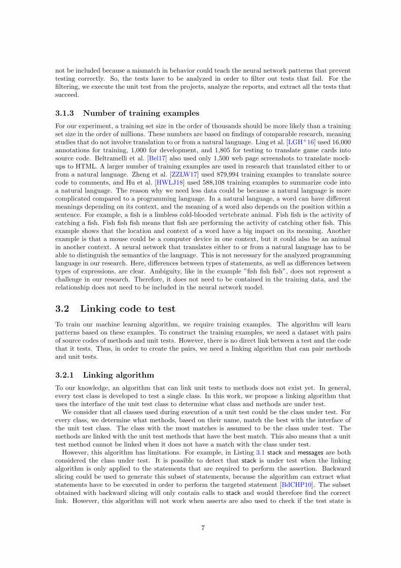
However, this algorithm has limitations. For example, in Listing 3.1 stack and messages are bothconsidered the class under test. It is possible to detect that stack is under test when the linkingalgorithm is only applied to the statements that are required to perform the assertion. Backwardslicing could be used to generate this subset of statements, because the algorithm can extract whatstatements have to be executed in order to perform the targeted statement [BdCHP10]. The subsetobtained with backward slicing will only contain calls to stack and would therefore find the correctlink. However, this algorithm will not work when asserts are also used to check if the test state is

7

valid to perform the operation that is tested, as now additional statements are included that havenothing to do with the method under test.

1 public void push() {2 ...3 stack = stack.push(133);4 messages.push(”Asserting”);5 assertEquals(133, stack.top());6 }

Listing 3.1: Unit tests that will be incorrectly linked without statement elimination

3.2.2 Linking methods

The linking algorithm of Section 3.2.1 could be used to construct the links. However, the algorithmrequires information about the source code as input. As described in Section 2.2, this could be doneby analyzing the AST or bytecode.

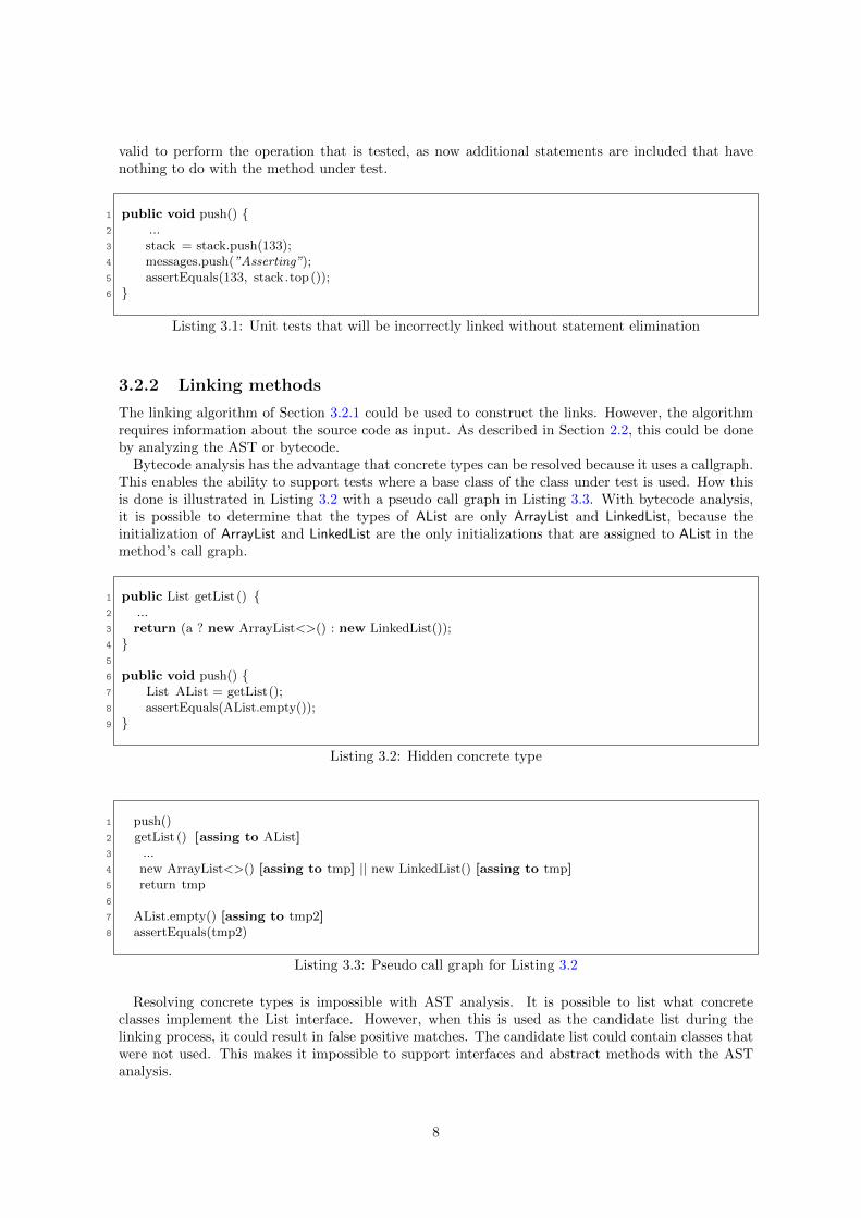
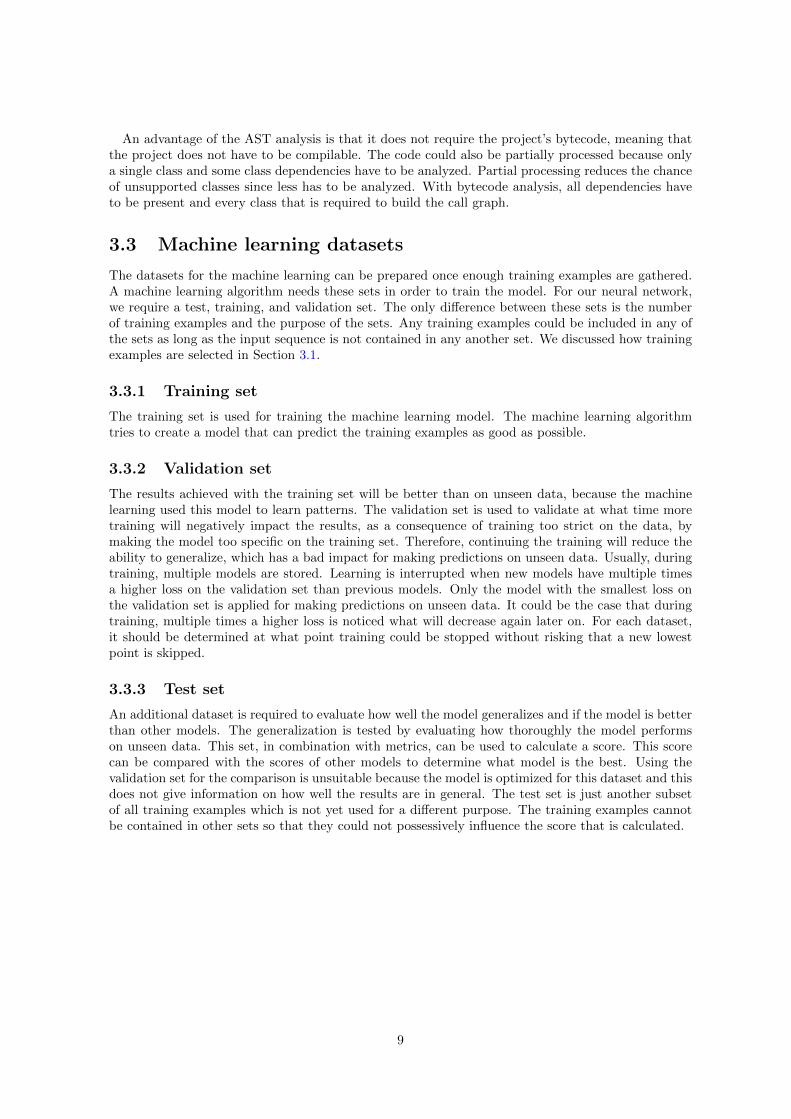
Bytecode analysis has the advantage that concrete types can be resolved because it uses a callgraph.This enables the ability to support tests where a base class of the class under test is used. How thisis done is illustrated in Listing 3.2 with a pseudo call graph in Listing 3.3. With bytecode analysis,it is possible to determine that the types of AList are only ArrayList and LinkedList, because theinitialization of ArrayList and LinkedList are the only initializations that are assigned to AList in themethod’s call graph.

1 public List getList() {2 ...3 return (a ? new ArrayList<>() : new LinkedList());4 }5

6 public void push() {7 List AList = getList();8 assertEquals(AList.empty());9 }

Listing 3.2: Hidden concrete type

1 push()2 getList () [assing to AList]3 ...4 new ArrayList<>() [assing to tmp] || new LinkedList() [assing to tmp]5 return tmp6

7 AList.empty() [assing to tmp2]8 assertEquals(tmp2)

Listing 3.3: Pseudo call graph for Listing 3.2

Resolving concrete types is impossible with AST analysis. It is possible to list what concreteclasses implement the List interface. However, when this is used as the candidate list during thelinking process, it could result in false positive matches. The candidate list could contain classes thatwere not used. This makes it impossible to support interfaces and abstract methods with the ASTanalysis.

8

An advantage of the AST analysis is that it does not require the project’s bytecode, meaning thatthe project does not have to be compilable. The code could also be partially processed because onlya single class and some class dependencies have to be analyzed. Partial processing reduces the chanceof unsupported classes since less has to be analyzed. With bytecode analysis, all dependencies haveto be present and every class that is required to build the call graph.

3.3 Machine learning datasets

The datasets for the machine learning can be prepared once enough training examples are gathered.A machine learning algorithm needs these sets in order to train the model. For our neural network,we require a test, training, and validation set. The only difference between these sets is the numberof training examples and the purpose of the sets. Any training examples could be included in any ofthe sets as long as the input sequence is not contained in any another set. We discussed how trainingexamples are selected in Section 3.1.

3.3.1 Training set

The training set is used for training the machine learning model. The machine learning algorithmtries to create a model that can predict the training examples as good as possible.

3.3.2 Validation set

The results achieved with the training set will be better than on unseen data, because the machinelearning used this model to learn patterns. The validation set is used to validate at what time moretraining will negatively impact the results, as a consequence of training too strict on the data, bymaking the model too specific on the training set. Therefore, continuing the training will reduce theability to generalize, which has a bad impact for making predictions on unseen data. Usually, duringtraining, multiple models are stored. Learning is interrupted when new models have multiple timesa higher loss on the validation set than previous models. Only the model with the smallest loss onthe validation set is applied for making predictions on unseen data. It could be the case that duringtraining, multiple times a higher loss is noticed what will decrease again later on. For each dataset,it should be determined at what point training could be stopped without risking that a new lowestpoint is skipped.

3.3.3 Test set

An additional dataset is required to evaluate how well the model generalizes and if the model is betterthan other models. The generalization is tested by evaluating how thoroughly the model performson unseen data. This set, in combination with metrics, can be used to calculate a score. This scorecan be compared with the scores of other models to determine what model is the best. Using thevalidation set for the comparison is unsuitable because the model is optimized for this dataset and thisdoes not give information on how well the results are in general. The test set is just another subsetof all training examples which is not yet used for a different purpose. The training examples cannotbe contained in other sets so that they could not possessively influence the score that is calculated.

9

Chapter 4

Evaluation Setup

For the evaluation of our approach, we introduce in total three goal metrics that indicate how far weare from generating working code to the ability to find bugs. However, the results of the metrics couldbe biased because we are using machine learning. The nodes of a neural network are initialized withrandom values before training starts. From this point, the network is optimized so that it can predictthe training set as good as possible. Different initial values will result in different clusters within theneural network, what impacts the prediction capabilities. This means that metric scores could be dueto chance. In this chapter, we will address this issue.

We created a baseline with selected test projects to enable comparisons of our results with thegenerated test suite of alternative test generators and manually written test suites. This baseline canbe used when unit tests can be generated. Otherwise, we do not have to use these projects. Theevaluation of any method is fine because we do not have to be able to calculate the effectiveness ofthe tests. In our research, for RQ1 we perform multiple experiments with different configurations(different datasets and different network configurations). We have to prove that a change in theconfiguration will result in a higher metric score. For RQ2 we prove that with compression theaccuracy will increase, and the required time will decrease.

4.1 Evaluation

The test suite capability should be evaluated if the generator can generate test code. Nevertheless,when the test generator is in a phase where it is unable to produce valid tests, a simple metric shouldbe applied which does not test the testing capability. However, it would qualify how far we are fromgenerating executable code because code that is not executable is unable to test something. Thisset of metrics enables us to make comparisons over the whole phase of the development of the testgenerator.

4.1.1 Metrics

The machine learning models can be compared to its ability to generate parsable code (parsable rate),compilable code (compilable rate), and code that can detect faults (mutation score). The parsablerate and compilable rate measure the test generator’s ability to write code. The difference betweenthese two is that compilable code is executable, while this is not necessarily true for parsable code.The mutation score measures the test generator’s test quality.

These metrics should be used in different phases. The mutation score should be used when themodel can generate working unit tests to measure the test suite effectiveness. The compilable codemetric should be used when the machine learning model is aware of the language’s grammar to measurethe ability of writing working code. If the mutation score and compilable code metric cannot be used,the parsable code metric should be applied. This measures how well the model knows the grammarof the programming language.

10

4.1.2 Measurement

The parsable rate can be measured by calculating the percentage of the code that can be parsedwith the grammar of the programming language. The parsable rate can be calculated by dividingthe amount of code that parses with the total amount of analyzed code. The same calculation as forparsable rate can be applied for the compilable rate. However, instead of parsing the code with thegrammar, the code should be compiled with a compiler.

The mutation score is measured by a fork of the PIT Mutation Testing1. This fork is used because itis combining multiple mutation generations, which leads to a more realistic mutation score [PMm17].

4.1.3 Comparing machine learning models

A machine learning model depends on random values. When we calculate metrics for a generated testsuite, the results will be different when we use another seed for the random number generator.

When we want to compare results with the metrics from Section 4.1, we have to cancel out theeffect of the random numbers. We do this by performing multiple experiments instead of runningsingle experiments. Then, we use statistics to test for significant differences between the two groupsof experiments. If there is a significant difference, we use statistics to prove that one group of resultsis significantly better than the other group of results.

4.2 Baseline

The effectiveness of a project’s manually written test suite and of automatically generated test suitesare used as the baseline. Only test suit generators that implement search-based testing and randomtesting are considered, because many open-source tools are available for these methods and they areoften used in related work. We use Evosuite2 for search-based testing and Randoop3 for randomtesting, as these are the highest scoring open-source test suite generators in the 2017 SBST Java UnitTesting Tool Competition in their respective categories [PM17].

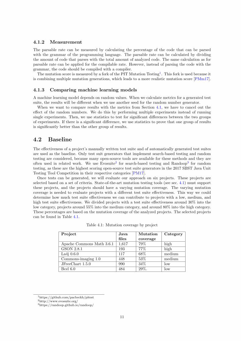
Once tests can be generated, we will evaluate our approach on six projects. These projects areselected based on a set of criteria. State-of-the-art mutation testing tools (see sec. 4.1) must supportthese projects, and the projects should have a varying mutation coverage. The varying mutationcoverage is needed to evaluate projects with a different test suite effectiveness. This way we coulddetermine how much test suite effectiveness we can contribute to projects with a low, medium, andhigh test suite effectiveness. We divided projects with a test suite effectiveness around 30% into thelow category, projects around 55% into the medium category, and around 80% into the high category.These percentages are based on the mutation coverage of the analyzed projects. The selected projectscan be found in Table 4.1.

Table 4.1: Mutation coverage by project

Project Javafiles

Mutationcoverage

Category

Apache Commons Math 3.6.1 1,617 79% highGSON 2.8.1 193 77% highLa4j 0.6.0 117 68% mediumCommons-imaging 1.0 448 53% mediumJFreeChart 1.5.0 990 34% lowBcel 6.0 484 29%. low

1https://github.com/pacbeckh/pitest2http://www.evosuite.org/3https://randoop.github.io/randoop/

11

Chapter 5

Experimental Setup

How a test suite generator can be developed in general was discussed in Chapter 3. The chaptercontains details on how training examples can be collected and explains how these examples can beused in machine learning models. How the test generator can be evaluated is discussed in Chapter 4.Several metrics are included, and a baseline is given. This chapter gives insight on how the test suitegenerator is developed for this research. We included additional criteria to simplify the development ofthe test generator. For instance, we only extract training examples from projects with a dependencymanager to relieve ourselves of manually building projects.

5.1 Data collection

Besides the criteria mentioned in Section 3.1, we added additional requirements to the projects wegathered to make the extraction of training data less time-consuming. We also used a project hostingwebsite to make the process of filtering and obtaining the projects less time-consuming.

5.1.1 Additional project criteria

It is time-consuming to execute the unit test suits for all projects manually. A dependency managercould be used to automate this for these projects. Projects that use a dependency manager use aconfiguration file that defines the requirements on how to build, and most of the time also on how toexecute the project’s unit tests. Therefore, we expect that only using projects that have a dependencymanager will make this task less time-consuming. We only consider Maven1 and Gradle2 because theseare the only dependency managers that are officially supported by JUnit [Juna].

5.1.2 Collecting projects

We use the GitHub3 platform to filter and obtain projects. GitHub has an API that can be usedto obtain a list of projects that meet specific requirements. However, the API has some limitations.Multiple requests have to be done to perform complex queries. Each query can show a maximumof 1,000 results which have to be retrieved in batches of maximum 100 results, and the number ofqueries is limited to 30 per minute [Git]. To cope with the limit of 1,000 results per query, we usedthe project size criteria to partition the projects into batches with a maximum of 1,000 projects perbatch. For our research, we need to make the following requests:

• As mentioned, we have to partition the projects to cope with the limitation of maximum 1,000results per query. The partitioning is performed by obtaining the Java projects starting from acertain project size and are obtained by performing 10 requests to get the results in batches of100. This step is repeated with an updated start size until all projects are obtained.

1https://maven.apache.org/2https://gradle.org/3https://github.com/

12

• For each project, a call has to be made to determine if the project uses JUnit in at least oneof their unit tests. This can be done by searching for test files that use JUnit. The project isexcluded when it does not meet this criterion.

• Additional calls have to be made to determine if the project has a build.gradle (for Gradleprojects) with the JUnit4 dependency or a pom.xml (for Maven projects) with the JUnit 4 de-pendency. An extra call is required for Maven projects to check if it has the JUnit 4 dependency.The dependency name ends either with junit4, or is called JUnit and has version 4.* inside theversion tag.

The number of requests needed for each operation could be used to limit the total number ofrequests required. This can improve the total time required for this process. In our case, we expectthat it is best to check first if a project is a Gradle project before checking if it is a Maven project,because more requests are required for Maven projects.

In conclusion, to list the available projects, one request has to be made for every 100 projects. Eachproject requires additional requests: one request to check if a project has tests, one additional requestfor projects that use Gradle, and at most two extra requests for projects that use Maven.

So, to analyze n projects, at minimum n ∗ ((1/100) + 1)/30 and at maximum n ∗ ((1/100) + 4)/30minutes are required.

5.1.3 Training data

With the GitHub API mentioned in Section 5.1.2, we analyzed 1,196,899 open-source projects. Fromthese projects, 3,385 complied with our criteria. We ended up with 1,106 projects after eliminating allprojects that could not be built or tested. These projects have in total 560,413 unit tests. These unittests could be used to create training examples. However, the total amount of training data could beless than the number of unit tests, because the linking algorithm might be unable to link every unittest (as described in Section 3.2.1).

5.2 Extraction training examples

The training example extraction can be performed with the linking algorithm described in Section3.2.1 by using the analysis techniques described in Section 3.2.2. For the extraction, we use thetraining projects mentioned in Section 5.1.1.

As mentioned in Section 5.1.3, we have to analyze a large number of training projects. For ourresearch, we lack the infrastructure to process all projects within a reasonable time. To make it possibleto process everything in phases, we introduced a queue. This enables us to interrupt processing atany time and continue it later without skipping any project. As mentioned in Section 3.1, we shouldonly include unit tests that succeeded. Thus, we fill the queue based on test reports. When all testreports are contained, we start linking small groups of tests until everything is processed.

5.2.1 Building the queue

The queue is used by both bytecode analysis and AST analysis. All the unit tests of each trainingproject are contained in the queue. We structured the queue in a manner so it contains all theinformation required for these tools. For instance, we have to store the classpath to perform bytecodeanalysis, the source location to perform AST analysis, and we have to store the unit test class nameand unit test method name for both bytecode and AST analysis.

The source location and classpath can be extracted based upon the name of the test class. Foreach test class, there exists a ”.class” and ”.java” file. The ”.class” file is inside the classpath, and the”.java” file is inside the source path. The root of these paths can be found based on the namespaceof the test class. Often, one level up from the classpath, there is a folder with other classpaths. Ifthis is the case, then usually there is a folder for the generated classes, test-classes, and the regularclasses. The classes used in the unit test could be in any of these folders. Therefore, all these pathshave to be included to perform a complete analysis.

13

The test class and test methods can be extracted based on the test report of each project. The testreport consists of test classes with the number of unit tests that succeeded and how many failed ordid not run for any other reason. From the report we cannot differentiate between test methods thatsucceeded or failed. So, we only consider test classes for which all test methods succeeded. The testmethods from the test class can be extracted by listing all methods with a @Test annotation insidethe test class.

5.3 Training machine learning models

The last step is to train the machine learning models. In order to train the machine learning model,we need to obtain a training and validation set. To evaluate how well the model performs, we use atest set. We divided the gathered training examples into these three sets. We use 80% of the data forthe training, 10% for the validation, and 10% for the test set.

However, the quality of a machine learning model does not only depend on the used training data. Italso depends on the data representation. In this section, we introduced four views, namely tokenizedview, compression, BPE [SHB15], and AST. From these views, the tokenized view resembles thetextual form of the data the most. The other views modify the presented information.

5.3.1 Tokenized view

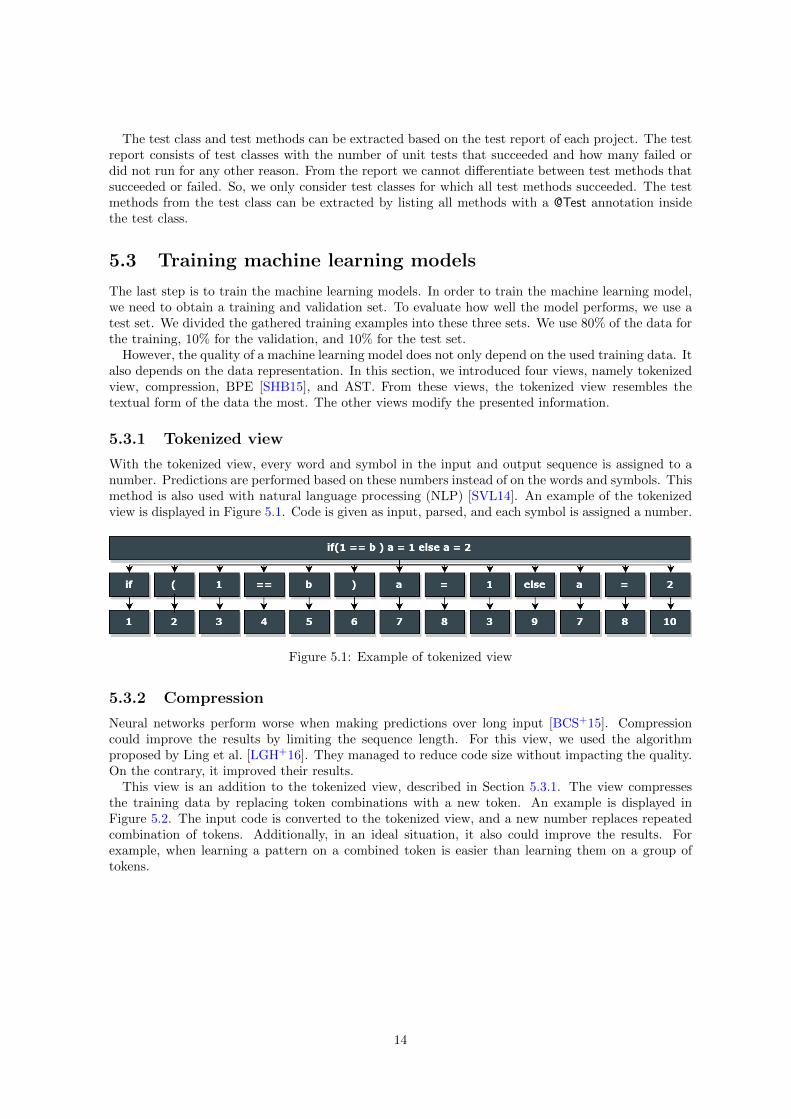
With the tokenized view, every word and symbol in the input and output sequence is assigned to anumber. Predictions are performed based on these numbers instead of on the words and symbols. Thismethod is also used with natural language processing (NLP) [SVL14]. An example of the tokenizedview is displayed in Figure 5.1. Code is given as input, parsed, and each symbol is assigned a number.

Figure 5.1: Example of tokenized view

5.3.2 Compression

Neural networks perform worse when making predictions over long input [BCS+15]. Compressioncould improve the results by limiting the sequence length. For this view, we used the algorithmproposed by Ling et al. [LGH+16]. They managed to reduce code size without impacting the quality.On the contrary, it improved their results.

This view is an addition to the tokenized view, described in Section 5.3.1. The view compressesthe training data by replacing token combinations with a new token. An example is displayed inFigure 5.2. The input code is converted to the tokenized view, and a new number replaces repeatedcombination of tokens. Additionally, in an ideal situation, it also could improve the results. Forexample, when learning a pattern on a combined token is easier than learning them on a group oftokens.

14

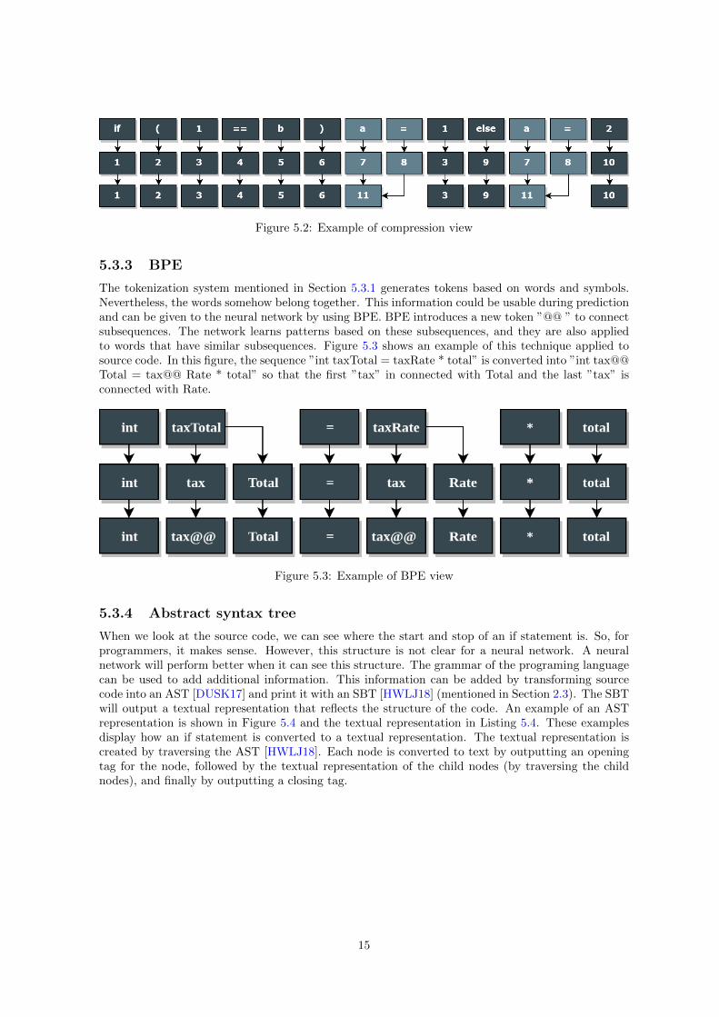
Figure 5.2: Example of compression view

5.3.3 BPE

The tokenization system mentioned in Section 5.3.1 generates tokens based on words and symbols.Nevertheless, the words somehow belong together. This information could be usable during predictionand can be given to the neural network by using BPE. BPE introduces a new token ”@@ ” to connectsubsequences. The network learns patterns based on these subsequences, and they are also appliedto words that have similar subsequences. Figure 5.3 shows an example of this technique applied tosource code. In this figure, the sequence ”int taxTotal = taxRate * total” is converted into ”int tax@@Total = tax@@ Rate * total” so that the first ”tax” in connected with Total and the last ”tax” isconnected with Rate.

Figure 5.3: Example of BPE view

5.3.4 Abstract syntax tree

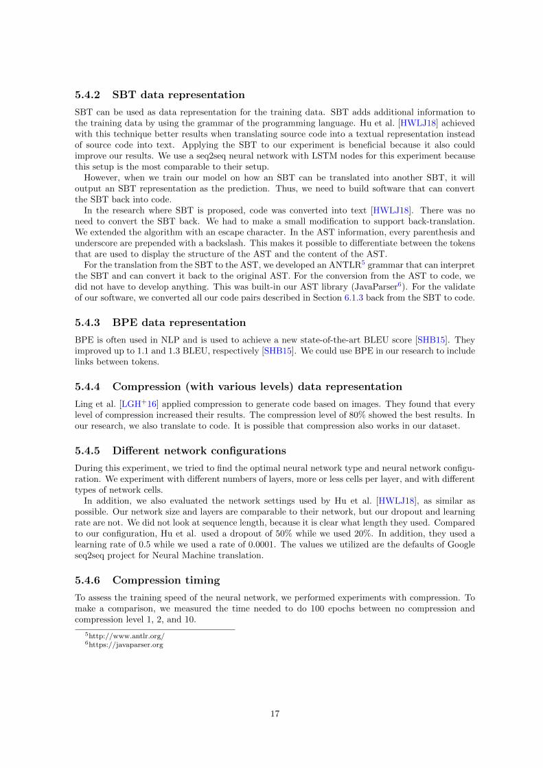
When we look at the source code, we can see where the start and stop of an if statement is. So, forprogrammers, it makes sense. However, this structure is not clear for a neural network. A neuralnetwork will perform better when it can see this structure. The grammar of the programing languagecan be used to add additional information. This information can be added by transforming sourcecode into an AST [DUSK17] and print it with an SBT [HWLJ18] (mentioned in Section 2.3). The SBTwill output a textual representation that reflects the structure of the code. An example of an ASTrepresentation is shown in Figure 5.4 and the textual representation in Listing 5.4. These examplesdisplay how an if statement is converted to a textual representation. The textual representation iscreated by traversing the AST [HWLJ18]. Each node is converted to text by outputting an openingtag for the node, followed by the textual representation of the child nodes (by traversing the childnodes), and finally by outputting a closing tag.

15

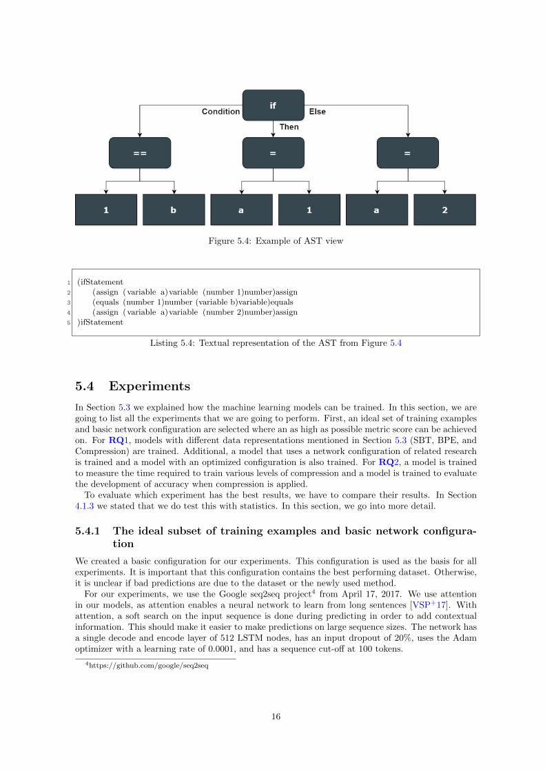
Figure 5.4: Example of AST view

1 (ifStatement2 (assign (variable a)variable (number 1)number)assign3 (equals (number 1)number (variable b)variable)equals4 (assign (variable a)variable (number 2)number)assign5 )ifStatement

Listing 5.4: Textual representation of the AST from Figure 5.4

5.4 Experiments

In Section 5.3 we explained how the machine learning models can be trained. In this section, we aregoing to list all the experiments that we are going to perform. First, an ideal set of training examplesand basic network configuration are selected where an as high as possible metric score can be achievedon. For RQ1, models with different data representations mentioned in Section 5.3 (SBT, BPE, andCompression) are trained. Additional, a model that uses a network configuration of related researchis trained and a model with an optimized configuration is also trained. For RQ2, a model is trainedto measure the time required to train various levels of compression and a model is trained to evaluatethe development of accuracy when compression is applied.

To evaluate which experiment has the best results, we have to compare their results. In Section4.1.3 we stated that we do test this with statistics. In this section, we go into more detail.

5.4.1 The ideal subset of training examples and basic network configura-tion

We created a basic configuration for our experiments. This configuration is used as the basis for allexperiments. It is important that this configuration contains the best performing dataset. Otherwise,it is unclear if bad predictions are due to the dataset or the newly used method.

For our experiments, we use the Google seq2seq project4 from April 17, 2017. We use attentionin our models, as attention enables a neural network to learn from long sentences [VSP+17]. Withattention, a soft search on the input sequence is done during predicting in order to add contextualinformation. This should make it easier to make predictions on large sequence sizes. The network hasa single decode and encode layer of 512 LSTM nodes, has an input dropout of 20%, uses the Adamoptimizer with a learning rate of 0.0001, and has a sequence cut-off at 100 tokens.

4https://github.com/google/seq2seq

16

5.4.2 SBT data representation

SBT can be used as data representation for the training data. SBT adds additional information tothe training data by using the grammar of the programming language. Hu et al. [HWLJ18] achievedwith this technique better results when translating source code into a textual representation insteadof source code into text. Applying the SBT to our experiment is beneficial because it also couldimprove our results. We use a seq2seq neural network with LSTM nodes for this experiment becausethis setup is the most comparable to their setup.

However, when we train our model on how an SBT can be translated into another SBT, it willoutput an SBT representation as the prediction. Thus, we need to build software that can convertthe SBT back into code.

In the research where SBT is proposed, code was converted into text [HWLJ18]. There was noneed to convert the SBT back. We had to make a small modification to support back-translation.We extended the algorithm with an escape character. In the AST information, every parenthesis andunderscore are prepended with a backslash. This makes it possible to differentiate between the tokensthat are used to display the structure of the AST and the content of the AST.

For the translation from the SBT to the AST, we developed an ANTLR5 grammar that can interpretthe SBT and can convert it back to the original AST. For the conversion from the AST to code, wedid not have to develop anything. This was built-in our AST library (JavaParser6). For the validateof our software, we converted all our code pairs described in Section 6.1.3 back from the SBT to code.

5.4.3 BPE data representation

BPE is often used in NLP and is used to achieve a new state-of-the-art BLEU score [SHB15]. Theyimproved up to 1.1 and 1.3 BLEU, respectively [SHB15]. We could use BPE in our research to includelinks between tokens.

5.4.4 Compression (with various levels) data representation

Ling et al. [LGH+16] applied compression to generate code based on images. They found that everylevel of compression increased their results. The compression level of 80% showed the best results. Inour research, we also translate to code. It is possible that compression also works in our dataset.

5.4.5 Different network configurations

During this experiment, we tried to find the optimal neural network type and neural network configu-ration. We experiment with different numbers of layers, more or less cells per layer, and with differenttypes of network cells.

In addition, we also evaluated the network settings used by Hu et al. [HWLJ18], as similar aspossible. Our network size and layers are comparable to their network, but our dropout and learningrate are not. We did not look at sequence length, because it is clear what length they used. Comparedto our configuration, Hu et al. used a dropout of 50% while we used 20%. In addition, they used alearning rate of 0.5 while we used a rate of 0.0001. The values we utilized are the defaults of Googleseq2seq project for Neural Machine translation.

5.4.6 Compression timing

To assess the training speed of the neural network, we performed experiments with compression. Tomake a comparison, we measured the time needed to do 100 epochs between no compression andcompression level 1, 2, and 10.

5http://www.antlr.org/6https://javaparser.org

17

5.4.7 Compression accuracy

We evaluated a compression level that is close to the original textual form to test the impact onaccuracy when using compression. When compression caused the model to not generate parsablecode, we looked at the development of loss over time. The loss represents how far the validation setis from predicting the truth. We can conclude that the model is not learning when the loss increasesfrom the start of the experiment. This would mean that compression does not work on our dataset.We have only used the compression level 1 dataset for this experiment.

5.4.8 Finding differences between experiments

For RQ1, we first perform all experiments to create an overview of the results. Then, we selectthe experiments which we want to test whether there is a significant different result. We only dothis for experiments that improved our previous scores. As already mentioned in Section 4.1.3, weperform the same experiments multiple times to enable statistical analysis on those groups of results.For RQ2, we evaluate the effect of accuracy and speed during compression. For the evaluation ofspeed, we measured 30 times the time that was needed to perform 100 epochs when applying nocompression and compression level 1, 2, and 10. The evaluation of the accuracy is performed with themetrics discussed in Section 4.1. For this experiment, we ran five tests with a baseline without anycompression, and with various levels of compression. However, when compression prevents the modelfrom learning, we analyze the evolution of the loss on the validation set (which is used to determinewhen training the model further should be stopped) as mentioned in Section 5.4.7. The experimentwas repeated five times.

The first step in comparing experiments is to prove that there is a significant difference between theresults of the experiments. If there is a difference, we use statistics to evaluate what groups introducedthe difference and what relation these differences have.

For evaluating this difference, we use hypothesis testing with analysis of variance (ANOVA), withh0: there is no significant difference between the experiments; h1: there is a significant difference.We use an alpha-value of 0.05 to give a direction to the most promising setup for our research. Asthere is only one variable in the data, we use the one-way version of ANOVA. For RQ1, the variableis the dataset, and for RQ2, the variable is either the level of compression when testing speed, thedataset when testing the accuracy, or, when accuracy cannot be measured, the epoch is the variablewhen evaluating the loss.

The experiment is repeated for five times at least. So, our experiments are groups of results.However, each run in an experiment depends on a variable. This is the epoch number for the speedmeasurement of RQ2. For all other experiments, this is a random value. We need ANOVA forrepeated-measures to analyze these independent groups.

Nevertheless, when applying ANOVA for repeated-measures, there is the assumption that the vari-ances between all groups have to be equal (sphericity) [MB89]. We violate this in our experiments.For instance, when we use a different random value, there is a different spread in outcomes becauseit depends on another variable. When this violation is made, this has to be corrected. We use theGreenhouse-Geisser correction [Abd10] to do this. The correction is done by adjusting the degrees offreedom in the ANOVA test to increase the accuracy of the p-value.

When we apply ANOVA with the correction, we can evaluate if we can reject the h0 hypothesis (nodifference between the groups). When we can reject it, then it tells us there is a difference betweenthe groups, without knowing where. To know what caused the difference, we need to do an additionaltest. This additional test is performed with the Tukey’s multiple comparison test. This test is usedto compare the differences between the means of each group. For this test, a correction is applied tocancel out the effect of multiple testing. The correction is needed because when more conclusions aremade, the more likely an error occurs. For example, when performing five experiments with an errorrate of X%, there is a change of 5X% that an error is made within the whole test.

When we know what group is different, we still have to find out which group of results is better.So, we want to prove that the mean of one group is greater than the means of another group. Totest this, we perform a one-tail t-test on each individual group. We adjust the alpha according tohow many tests we perform on the same dataset to cancel out the effect of repeated measures. When

18

performing X tests, we divide the alpha by X to keep the total maximum error rate at 5%.

19

Chapter 6

Results

In Chapter 3 and Chapter 5, it is discussed how our experiments are performed in order to answerRQ1 and RQ2. In this chapter, we report on the obtained results. In Addition, we also report ontechniques used to generate training sets. This does not directly answer a research question. However,the training examples are both used to train models for both RQ1 and RQ2.

6.1 Linking experiments

In this section, we report on the linking algorithm described in Section 3.2.1. We mentioned in 3.2.2that both bytecode analysis and AST analysis use different principles, that might have a positiveimpact on their linking capabilities. We run both bytecode analysis and AST analysis on the queuementioned in Section 5.2. We assessed how many unit tests are supported by both techniques, howmany links both techniques can make on the same dataset, how many links both techniques can makein total, and what contradictory links were made between both techniques.

6.1.1 Removing redundant tests

The projects in our dataset, described in Section 5.1.3, contains 560,413 unit tests in total. However,there are duplicate projects in this dataset. To perform a reliable analysis, we have to remove duplicateunit tests. Otherwise, when a technique supports an additional link, it could be counted as more thanone extra link. The duplicates are removed based on their package name, class name, and test name.There remain 175,943 unit tests after removing the duplicates.

Unfortunately, this method will not eliminate duplicates when the name of the unit test, class, orpackage is changed, but it will remove duplicate tests when they have the same package, class andmethod name by coincidence. Thus, the algorithm removes methods with the same naming even whenthe implementation is different.

6.1.2 Unit test support

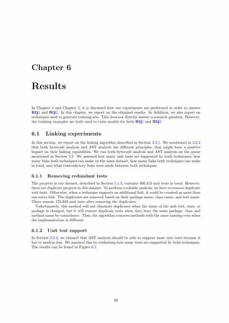
In Section 3.2.2, we claimed that AST analysis should be able to support more unit tests because ithas to analyze less. We assessed this by evaluating how many tests are supported by both techniques.The results can be found in Figure 6.1.

20

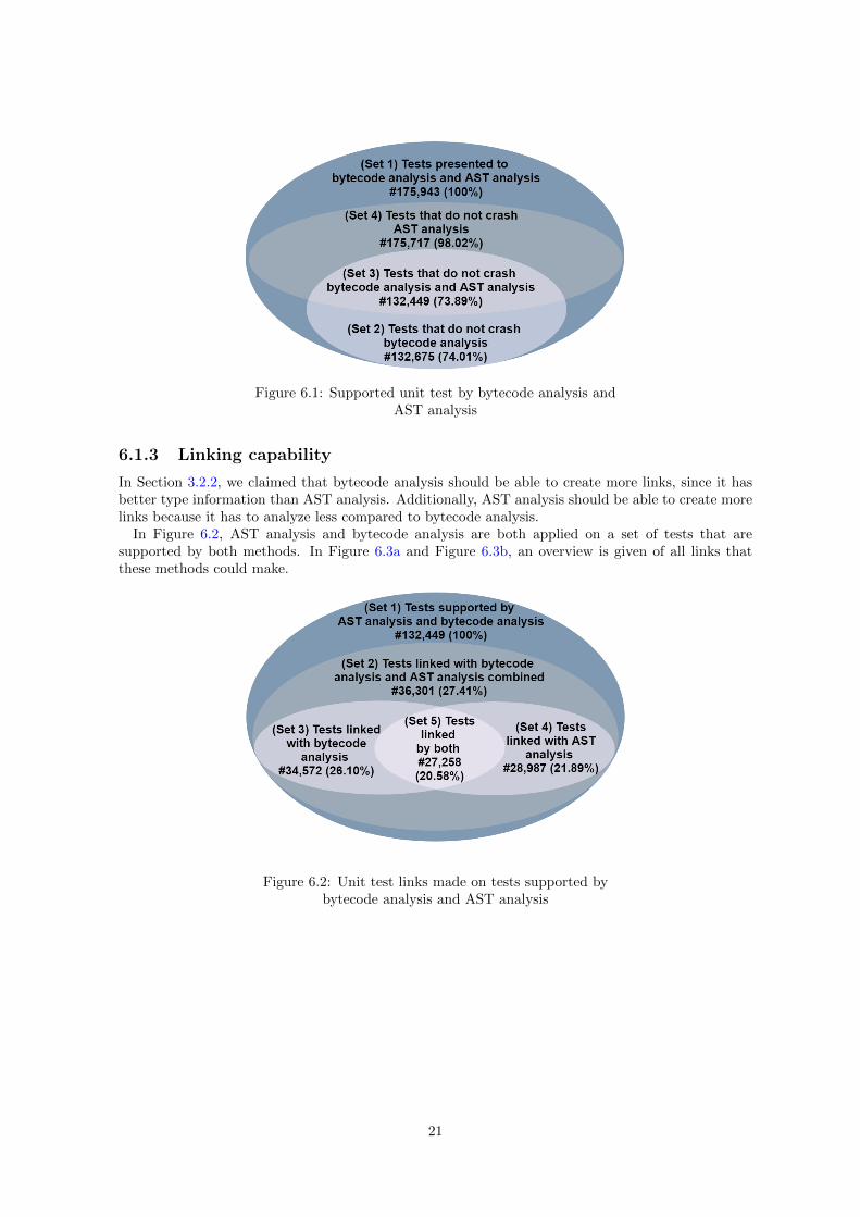
Figure 6.1: Supported unit test by bytecode analysis andAST analysis

6.1.3 Linking capability

In Section 3.2.2, we claimed that bytecode analysis should be able to create more links, since it hasbetter type information than AST analysis. Additionally, AST analysis should be able to create morelinks because it has to analyze less compared to bytecode analysis.

In Figure 6.2, AST analysis and bytecode analysis are both applied on a set of tests that aresupported by both methods. In Figure 6.3a and Figure 6.3b, an overview is given of all links thatthese methods could make.

Figure 6.2: Unit test links made on tests supported bybytecode analysis and AST analysis

21

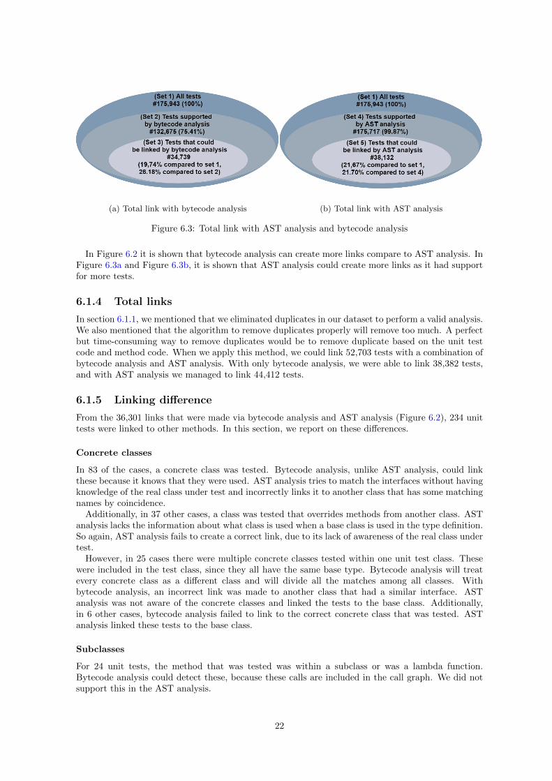
(a) Total link with bytecode analysis (b) Total link with AST analysis

Figure 6.3: Total link with AST analysis and bytecode analysis

In Figure 6.2 it is shown that bytecode analysis can create more links compare to AST analysis. InFigure 6.3a and Figure 6.3b, it is shown that AST analysis could create more links as it had supportfor more tests.

6.1.4 Total links

In section 6.1.1, we mentioned that we eliminated duplicates in our dataset to perform a valid analysis.We also mentioned that the algorithm to remove duplicates properly will remove too much. A perfectbut time-consuming way to remove duplicates would be to remove duplicate based on the unit testcode and method code. When we apply this method, we could link 52,703 tests with a combination ofbytecode analysis and AST analysis. With only bytecode analysis, we were able to link 38,382 tests,and with AST analysis we managed to link 44,412 tests.

6.1.5 Linking difference

From the 36,301 links that were made via bytecode analysis and AST analysis (Figure 6.2), 234 unittests were linked to other methods. In this section, we report on these differences.

Concrete classes

In 83 of the cases, a concrete class was tested. Bytecode analysis, unlike AST analysis, could linkthese because it knows that they were used. AST analysis tries to match the interfaces without havingknowledge of the real class under test and incorrectly links it to another class that has some matchingnames by coincidence.

Additionally, in 37 other cases, a class was tested that overrides methods from another class. ASTanalysis lacks the information about what class is used when a base class is used in the type definition.So again, AST analysis fails to create a correct link, due to its lack of awareness of the real class undertest.

However, in 25 cases there were multiple concrete classes tested within one unit test class. Thesewere included in the test class, since they all have the same base type. Bytecode analysis will treatevery concrete class as a different class and will divide all the matches among all classes. Withbytecode analysis, an incorrect link was made to another class that had a similar interface. ASTanalysis was not aware of the concrete classes and linked the tests to the base class. Additionally,in 6 other cases, bytecode analysis failed to link to the correct concrete class that was tested. ASTanalysis linked these tests to the base class.

Subclasses

For 24 unit tests, the method that was tested was within a subclass or was a lambda function.Bytecode analysis could detect these, because these calls are included in the call graph. We did notsupport this in the AST analysis.

22

Unfortunately, this also has disadvantages. In 14 other cases mocking was used. Bytecode analysisknew that a mock object was used and linked some tests to the mock object. However, the mockobject is not tested. The unit tests validated, for example, that a specific method was called duringthe unit test. Bytecode analysis incorrectly linked the test with the method that should be called andnot the method that made the call. AST analysis did not recognize the mock objects, and thereforeit could link the test to the method that was under test.

Unclear naming

The naming of a unit test does not always match the intent of the unit test. In 13 cases, multiplemethods were tested in the unit test. We only allowed our analysis tools to link to one method. BothAST analysis and bytecode analysis were correct, but they selected a different method. In 19 casesfor AST analysis and 3 cases for bytecode analysis, an incorrect method was linked because of unclearnaming. In 8 cases, it was not clear what method performed the operation that was tested. Multiplemethods could do the operation. In 2 cases, it was not clear what was tested.

6.2 Experiments for RQ1

All executed experiments are combined into the roadmap shown in Figure 6.4. Experiments are builton-top of the configuration of a previous category when it improves the latest results. We start witha training a model on all training examples, followed by the experiments discussed in Section 5.4.8.These experiments can be categorized into simplifications, combination of simplifications, differentdata representations, and different network configurations.

23

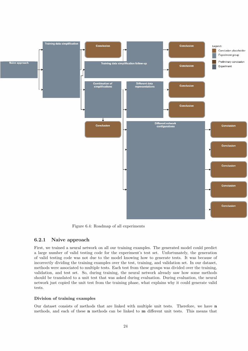
Figure 6.4: Roadmap of all experiments

6.2.1 Naive approach

First, we trained a neural network on all our training examples. The generated model could predicta large number of valid testing code for the experiment’s test set. Unfortunately, the generationof valid testing code was not due to the model knowing how to generate tests. It was because ofincorrectly dividing the training examples over the test, training, and validation set. In our dataset,methods were associated to multiple tests. Each test from these groups was divided over the training,validation, and test set. So, during training, the neural network already saw how some methodsshould be translated to a unit test that was asked during evaluation. During evaluation, the neuralnetwork just copied the unit test from the training phase, what explains why it could generate validtests.

Division of training examples

Our dataset consists of methods that are linked with multiple unit tests. Therefore, we have nmethods, and each of these n methods can be linked to m different unit tests. This means that

24

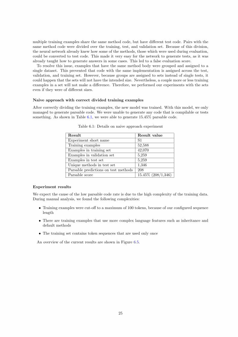
multiple training examples share the same method code, but have different test code. Pairs with thesame method code were divided over the training, test, and validation set. Because of this division,the neural network already knew how some of the methods, those which were used during evaluation,could be converted to test code. This made it very easy for the network to generate tests, as it wasalready taught how to generate answers in some cases. This led to a false evaluation score.

To resolve this issue, examples that have the same method body were grouped and assigned to asingle dataset. This prevented that code with the same implementation is assigned across the test,validation, and training set. However, because groups are assigned to sets instead of single tests, itcould happen that the sets will not have the intended size. Nevertheless, a couple more or less trainingexamples in a set will not make a difference. Therefore, we performed our experiments with the setseven if they were of different sizes.

Naive approach with correct divided training examples

After correctly dividing the training examples, the new model was trained. With this model, we onlymanaged to generate parsable code. We were unable to generate any code that is compilable or testssomething. As shown in Table 6.1, we were able to generate 15.45% parsable code.

Table 6.1: Details on naive approach experiment

Result Result valueExperiment short name S1Training examples 52,588Examples in training set 42,070Examples in validation set 5,259Examples in test set 5,259Unique methods in test set 1,346Parsable predictions on test methods 208Parsable score 15.45% (208/1,346)

Experiment results

We expect the cause of the low parsable code rate is due to the high complexity of the training data.During manual analysis, we found the following complexities:

• Training examples were cut-off to a maximum of 100 tokens, because of our configured sequencelength

• There are training examples that use more complex language features such as inheritance anddefault methods

• The training set contains token sequences that are used only once

An overview of the current results are shown in Figure 6.5.

25

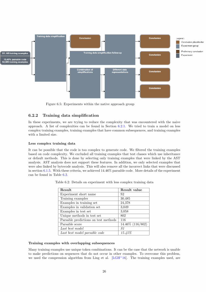
Figure 6.5: Experiments within the native approach group

6.2.2 Training data simplification

In these experiments, we are trying to reduce the complexity that was encountered with the naiveapproach. A list of complexities can be found in Section 6.2.1. We tried to train a model on lesscomplex training examples, training examples that have common subsequences, and training exampleswith a limited size.

Less complex training data

It can be possible that the code is too complex to generate code. We filtered the training examplesbased on code complexity. We excluded all training examples that test classes which use inheritanceor default methods. This is done by selecting only training examples that were linked by the ASTanalysis. AST analysis does not support these features. In addition, we only selected examples thatwere also linked by bytecode analysis. This will also remove all the incorrect links that were discussedin section 6.1.5. With these criteria, we achieved 14.46% parsable code. More details of the experimentcan be found in Table 6.2.

Table 6.2: Details on experiment with less complex training data

Result Result valueExperiment short name S2Training examples 30,485Examples in training set 24,378Examples in validation set 3,049Examples in test set 3,058Unique methods in test set 802Parsable predictions on test methods 116Parsable score 14.46% (116/802)Last best model S1Last best model parsable code 15.45%

Training examples with overlapping subsequences

Many training examples use unique token combinations. It can be the case that the network is unableto make predictions on sequences that do not occur in other examples. To overcome this problem,we used the compression algorithm from Ling et al. [LGH+16]. The training examples used, are

26

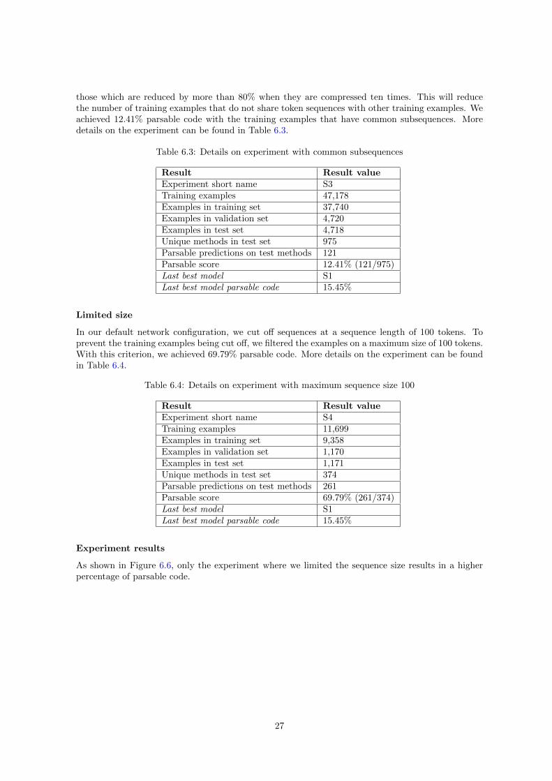
those which are reduced by more than 80% when they are compressed ten times. This will reducethe number of training examples that do not share token sequences with other training examples. Weachieved 12.41% parsable code with the training examples that have common subsequences. Moredetails on the experiment can be found in Table 6.3.

Table 6.3: Details on experiment with common subsequences

Result Result valueExperiment short name S3Training examples 47,178Examples in training set 37,740Examples in validation set 4,720Examples in test set 4,718Unique methods in test set 975Parsable predictions on test methods 121Parsable score 12.41% (121/975)Last best model S1Last best model parsable code 15.45%

Limited size

In our default network configuration, we cut off sequences at a sequence length of 100 tokens. Toprevent the training examples being cut off, we filtered the examples on a maximum size of 100 tokens.With this criterion, we achieved 69.79% parsable code. More details on the experiment can be foundin Table 6.4.

Table 6.4: Details on experiment with maximum sequence size 100

Result Result valueExperiment short name S4Training examples 11,699Examples in training set 9,358Examples in validation set 1,170Examples in test set 1,171Unique methods in test set 374Parsable predictions on test methods 261Parsable score 69.79% (261/374)Last best model S1Last best model parsable code 15.45%

Experiment results

As shown in Figure 6.6, only the experiment where we limited the sequence size results in a higherpercentage of parsable code.

27

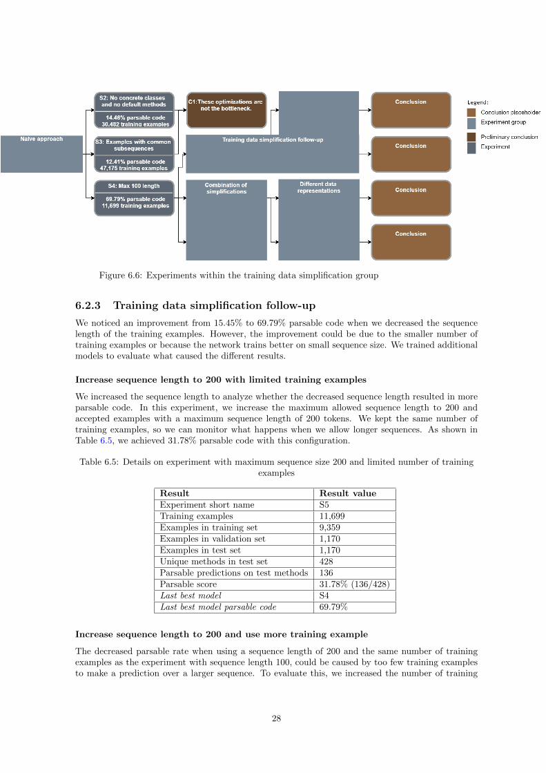
Figure 6.6: Experiments within the training data simplification group

6.2.3 Training data simplification follow-up

We noticed an improvement from 15.45% to 69.79% parsable code when we decreased the sequencelength of the training examples. However, the improvement could be due to the smaller number oftraining examples or because the network trains better on small sequence size. We trained additionalmodels to evaluate what caused the different results.

Increase sequence length to 200 with limited training examples

We increased the sequence length to analyze whether the decreased sequence length resulted in moreparsable code. In this experiment, we increase the maximum allowed sequence length to 200 andaccepted examples with a maximum sequence length of 200 tokens. We kept the same number oftraining examples, so we can monitor what happens when we allow longer sequences. As shown inTable 6.5, we achieved 31.78% parsable code with this configuration.

Table 6.5: Details on experiment with maximum sequence size 200 and limited number of trainingexamples

Result Result valueExperiment short name S5Training examples 11,699Examples in training set 9,359Examples in validation set 1,170Examples in test set 1,170Unique methods in test set 428Parsable predictions on test methods 136Parsable score 31.78% (136/428)Last best model S4Last best model parsable code 69.79%

Increase sequence length to 200 and use more training example

The decreased parsable rate when using a sequence length of 200 and the same number of trainingexamples as the experiment with sequence length 100, could be caused by too few training examplesto make a prediction over a larger sequence. To evaluate this, we increased the number of training

28

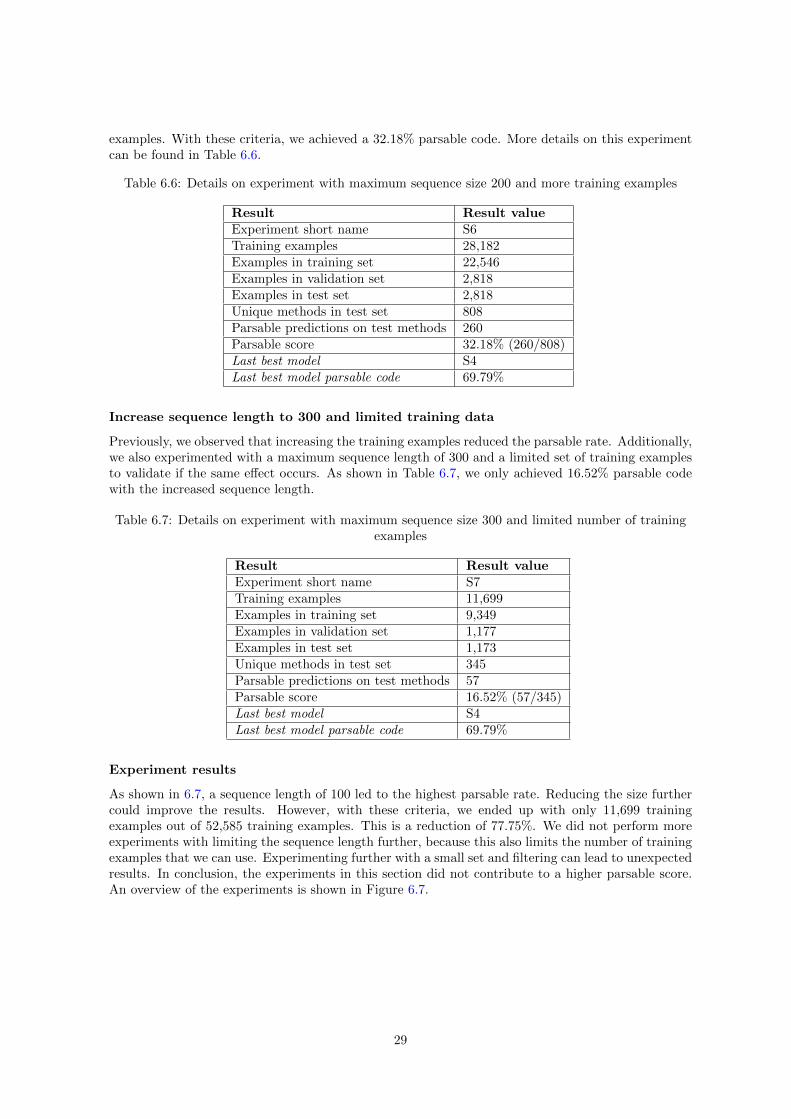
examples. With these criteria, we achieved a 32.18% parsable code. More details on this experimentcan be found in Table 6.6.

Table 6.6: Details on experiment with maximum sequence size 200 and more training examples

Result Result valueExperiment short name S6Training examples 28,182Examples in training set 22,546Examples in validation set 2,818Examples in test set 2,818Unique methods in test set 808Parsable predictions on test methods 260Parsable score 32.18% (260/808)Last best model S4Last best model parsable code 69.79%

Increase sequence length to 300 and limited training data

Previously, we observed that increasing the training examples reduced the parsable rate. Additionally,we also experimented with a maximum sequence length of 300 and a limited set of training examplesto validate if the same effect occurs. As shown in Table 6.7, we only achieved 16.52% parsable codewith the increased sequence length.

Table 6.7: Details on experiment with maximum sequence size 300 and limited number of trainingexamples

Result Result valueExperiment short name S7Training examples 11,699Examples in training set 9,349Examples in validation set 1,177Examples in test set 1,173Unique methods in test set 345Parsable predictions on test methods 57Parsable score 16.52% (57/345)Last best model S4Last best model parsable code 69.79%

Experiment results

As shown in 6.7, a sequence length of 100 led to the highest parsable rate. Reducing the size furthercould improve the results. However, with these criteria, we ended up with only 11,699 trainingexamples out of 52,585 training examples. This is a reduction of 77.75%. We did not perform moreexperiments with limiting the sequence length further, because this also limits the number of trainingexamples that we can use. Experimenting further with a small set and filtering can lead to unexpectedresults. In conclusion, the experiments in this section did not contribute to a higher parsable score.An overview of the experiments is shown in Figure 6.7.

29

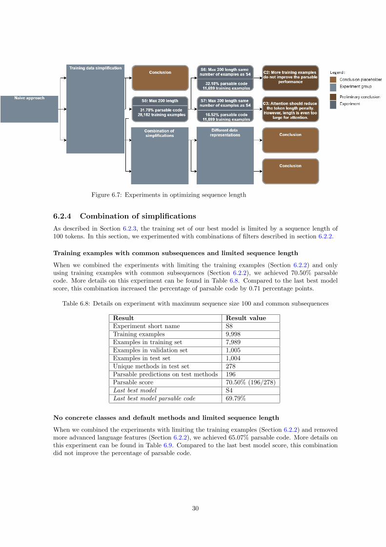
Figure 6.7: Experiments in optimizing sequence length

6.2.4 Combination of simplifications

As described in Section 6.2.3, the training set of our best model is limited by a sequence length of100 tokens. In this section, we experimented with combinations of filters described in section 6.2.2.

Training examples with common subsequences and limited sequence length

When we combined the experiments with limiting the training examples (Section 6.2.2) and onlyusing training examples with common subsequences (Section 6.2.2), we achieved 70.50% parsablecode. More details on this experiment can be found in Table 6.8. Compared to the last best modelscore, this combination increased the percentage of parsable code by 0.71 percentage points.

Table 6.8: Details on experiment with maximum sequence size 100 and common subsequences

Result Result valueExperiment short name S8Training examples 9,998Examples in training set 7,989Examples in validation set 1,005Examples in test set 1,004Unique methods in test set 278Parsable predictions on test methods 196Parsable score 70.50% (196/278)Last best model S4Last best model parsable code 69.79%

No concrete classes and default methods and limited sequence length

When we combined the experiments with limiting the training examples (Section 6.2.2) and removedmore advanced language features (Section 6.2.2), we achieved 65.07% parsable code. More details onthis experiment can be found in Table 6.9. Compared to the last best model score, this combinationdid not improve the percentage of parsable code.

30

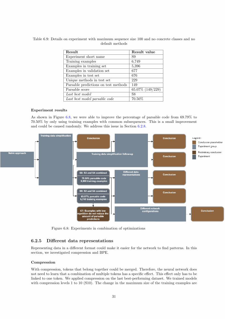
Table 6.9: Details on experiment with maximum sequence size 100 and no concrete classes and nodefault methods

Result Result valueExperiment short name S9Training examples 6,749Examples in training set 5,396Examples in validation set 677Examples in test set 676Unique methods in test set 229Parsable predictions on test methods 149Parsable score 65.07% (149/229)Last best model S8Last best model parsable code 70.50%

Experiment results

As shown in Figure 6.8, we were able to improve the percentage of parsable code from 69.79% to70.50% by only using training examples with common subsequences. This is a small improvementand could be caused randomly. We address this issue in Section 6.2.8.

Figure 6.8: Experiments in combination of optimizations

6.2.5 Different data representations

Representing data in a different format could make it easier for the network to find patterns. In thissection, we investigated compression and BPE.

Compression

With compression, tokens that belong together could be merged. Therefore, the neural network doesnot need to learn that a combination of multiple tokens has a specific effect. This effect only has to belinked to one token. We applied compression on the last best-performing dataset. We trained modelswith compression levels 1 to 10 (S10). The change in the maximum size of the training examples are

31

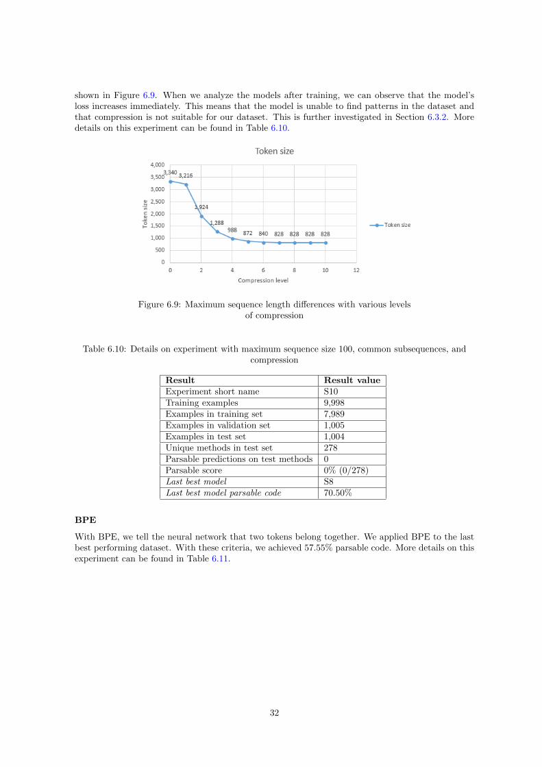
shown in Figure 6.9. When we analyze the models after training, we can observe that the model’sloss increases immediately. This means that the model is unable to find patterns in the dataset andthat compression is not suitable for our dataset. This is further investigated in Section 6.3.2. Moredetails on this experiment can be found in Table 6.10.

Figure 6.9: Maximum sequence length differences with various levelsof compression

Table 6.10: Details on experiment with maximum sequence size 100, common subsequences, andcompression

Result Result valueExperiment short name S10Training examples 9,998Examples in training set 7,989Examples in validation set 1,005Examples in test set 1,004Unique methods in test set 278Parsable predictions on test methods 0Parsable score 0% (0/278)Last best model S8Last best model parsable code 70.50%

BPE

With BPE, we tell the neural network that two tokens belong together. We applied BPE to the lastbest performing dataset. With these criteria, we achieved 57.55% parsable code. More details on thisexperiment can be found in Table 6.11.

32

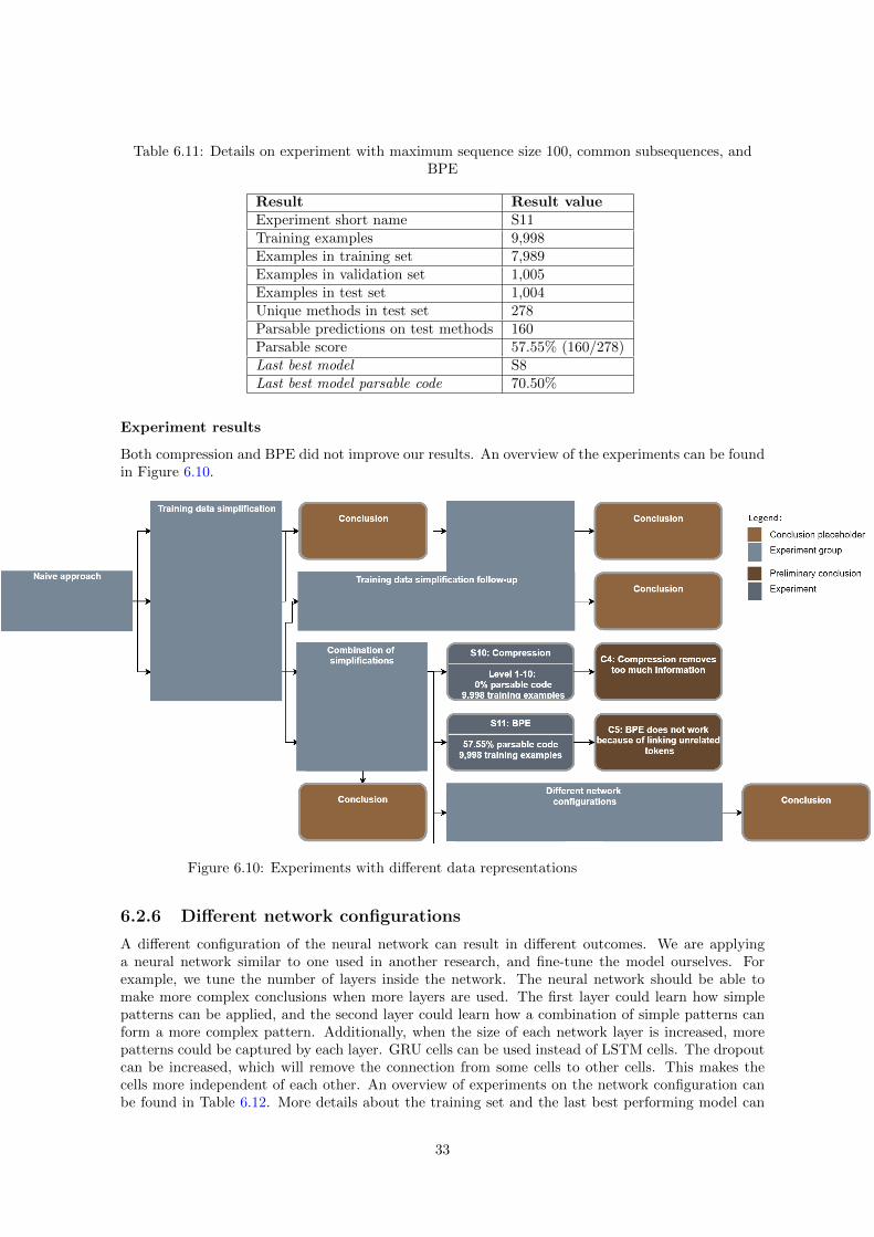
Table 6.11: Details on experiment with maximum sequence size 100, common subsequences, andBPE

Result Result valueExperiment short name S11Training examples 9,998Examples in training set 7,989Examples in validation set 1,005Examples in test set 1,004Unique methods in test set 278Parsable predictions on test methods 160Parsable score 57.55% (160/278)Last best model S8Last best model parsable code 70.50%

Experiment results

Both compression and BPE did not improve our results. An overview of the experiments can be foundin Figure 6.10.

Figure 6.10: Experiments with different data representations

6.2.6 Different network configurations

A different configuration of the neural network can result in different outcomes. We are applyinga neural network similar to one used in another research, and fine-tune the model ourselves. Forexample, we tune the number of layers inside the network. The neural network should be able tomake more complex conclusions when more layers are used. The first layer could learn how simplepatterns can be applied, and the second layer could learn how a combination of simple patterns canform a more complex pattern. Additionally, when the size of each network layer is increased, morepatterns could be captured by each layer. GRU cells can be used instead of LSTM cells. The dropoutcan be increased, which will remove the connection from some cells to other cells. This makes thecells more independent of each other. An overview of experiments on the network configuration canbe found in Table 6.12. More details about the training set and the last best performing model can

33

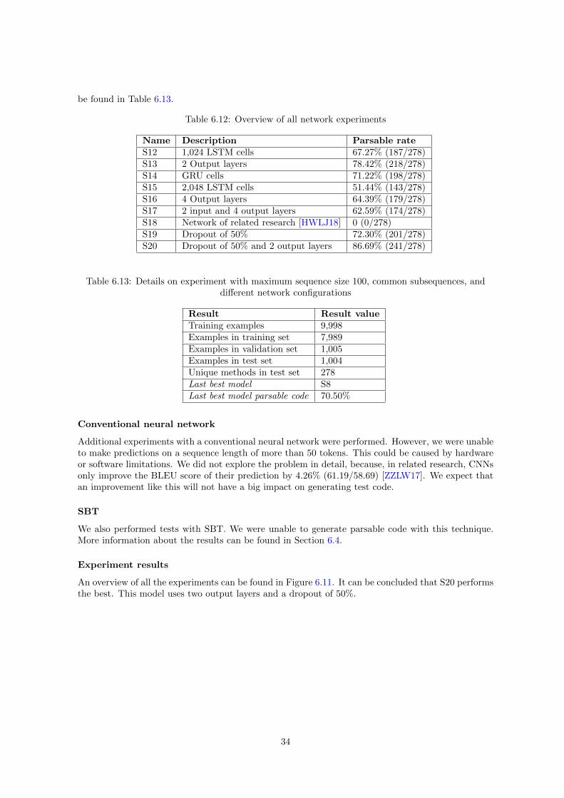
be found in Table 6.13.

Table 6.12: Overview of all network experiments

Name Description Parsable rateS12 1,024 LSTM cells 67.27% (187/278)S13 2 Output layers 78.42% (218/278)S14 GRU cells 71.22% (198/278)S15 2,048 LSTM cells 51.44% (143/278)S16 4 Output layers 64.39% (179/278)S17 2 input and 4 output layers 62.59% (174/278)S18 Network of related research [HWLJ18] 0 (0/278)S19 Dropout of 50% 72.30% (201/278)S20 Dropout of 50% and 2 output layers 86.69% (241/278)

Table 6.13: Details on experiment with maximum sequence size 100, common subsequences, anddifferent network configurations

Result Result valueTraining examples 9,998Examples in training set 7,989Examples in validation set 1,005Examples in test set 1,004Unique methods in test set 278Last best model S8Last best model parsable code 70.50%

Conventional neural network

Additional experiments with a conventional neural network were performed. However, we were unableto make predictions on a sequence length of more than 50 tokens. This could be caused by hardwareor software limitations. We did not explore the problem in detail, because, in related research, CNNsonly improve the BLEU score of their prediction by 4.26% (61.19/58.69) [ZZLW17]. We expect thatan improvement like this will not have a big impact on generating test code.

SBT

We also performed tests with SBT. We were unable to generate parsable code with this technique.More information about the results can be found in Section 6.4.

Experiment results

An overview of all the experiments can be found in Figure 6.11. It can be concluded that S20 performsthe best. This model uses two output layers and a dropout of 50%.

34

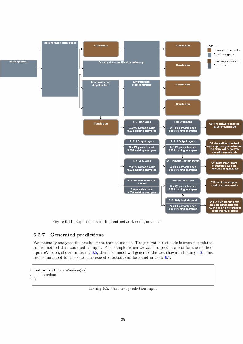
Figure 6.11: Experiments in different network configurations

6.2.7 Generated predictions

We manually analyzed the results of the trained models. The generated test code is often not relatedto the method that was used as input. For example, when we want to predict a test for the methodupdateVersion, shown in Listing 6.5, then the model will generate the test shown in Listing 6.6. Thistest is unrelated to the code. The expected output can be found in Code 6.7.

1 public void updateVersion() {2 ++version;3 }

Listing 6.5: Unit test prediction input

35

1 @Test public void testGetSequence() {2 assertEquals(1, m SIZE.getBytes());3 }

Listing 6.6: The generated unit test

1 @Test public void testUpdateVersion() {2 target .updateVersion();3 String result = target.getVersion();4 assertThat(result , is (”1”));5 }

Listing 6.7: Expected unit test

6.2.8 Experiment analysis

An overview of all experiments is shown in Figure 6.12.

36

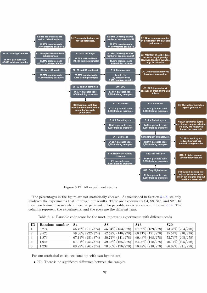
Figure 6.12: All experiment results

The percentages in the figure are not statistically checked. As mentioned in Section 5.4.8, we onlyanalyzed the experiments that improved our results. These are experiments S4, S8, S13, and S20. Intotal, we trained five models for each experiment. The parsable scores are shown in Table: 6.14. Thecolumns represent the experiments, and the rows are the different runs.

Table 6.14: Parsable code score for the most important experiments with different seeds

ID Random number S4 S8 S13 S201 5,274 56.42% (211/374) 55.04% (153/278) 67.99% (189/278) 73.38% (204/278)2 8,526 59.36% (222/374) 52.52% (146/278) 68.71% (191/278) 75.54% (210/278)3 1,873 67.11% (251/374) 50.72% (141/278) 60.43% (168/278) 73.74% (205/278)4 1,944 67.91% (254/374) 59.35% (165/278) 64.03% (178/278) 70.14% (195/278)5 1,234 69.79% (261/374) 70.50% (196/278) 78.42% (218/278) 86.69% (241/278)

For our statistical check, we came up with two hypotheses:

• H0: There is no significant difference between the samples

37

• H1: There is a significant difference between the samples

We apply the algorithms discussed in Section 5.4.8 to evaluate if H0 can be rejected. The resultsof the experiments can be found in Table: 6.15. We have a p-value lower than 0.05, so we can rejectH0. This means that there is a difference between the groups.

Table 6.15: ANOVA experiment results

Source of variation Sum of squares Degrees offreedom

Mean square F-value p-value

Between groups 873.6 3 291.2 15.9 0.0030Within groups 509.8 4 127.4 7.0 0.0039Residual 219.7 12 18.3Total 1.6 19

We apply the algorithms discussed in Section 5.4.8 to evaluate what the differences in results are.The results of the experiments can be found in Table: 6.16. We can reject H0 for the experimentsthat have a p-value lower than 0.05. That means that there is a statistically significant differencebetween S8 and S13, S8 and S20, and S13 and S20.

In Section 6.2.4, we discussed that common subsequences with a maximum sequence length of 100(S8) improved the parsable score of a maximum sequence length of 100 (S4) by 0.71 percentage points.When we calculate the averages of the follow-up experiments in Table 6.14, then S4 has an averageof 57.63%, while S8 has an average of 64.12%. We did not find a significant difference between theseexperiments. Therefore, we cannot conclude what filter on the dataset is better.

Table 6.16: Difference between experiments

Experiment Mean Difference 95% confidenceinterval ofdifference

Adjusted p-value

S4 vs. S8 6.492 -5.739 to 18.72 0.2757S4 vs. S13 −3.796 -19.12 to 11.53 0.7544S4 vs. S20 −11.78 -24.34 to 0.774 0.0612S8 vs. S13 −10.29 -18.40 to -2.180 0.0225S8 vs. S20 −18.27 -27.62 to -8.927 0.0047S13 vs. S20 −7.986 -13.74 to -2.232 0.0164

As shown in Table 6.16, S20 should have better results than S8 and S13, and S13 should have betterresults than S8. We came up with the following hypothesis for the directional t-test:

• H0: There is no significant difference between the results of Sx and Sy

• H1: The results of Sx are significantly higher than the results of Sy

We apply the directional t-test discussed in Section 5.4.8 to evaluate the hypothesis. The resultsare displayed in Table 6.17. For these experiments, we corrected the alpha to 0.05/3 to keep the samechance on an error. In these tables, it is shown that the p-value is lower than 0.02 (0.05/3). Thismeans that H0 can be rejected in all cases.

38

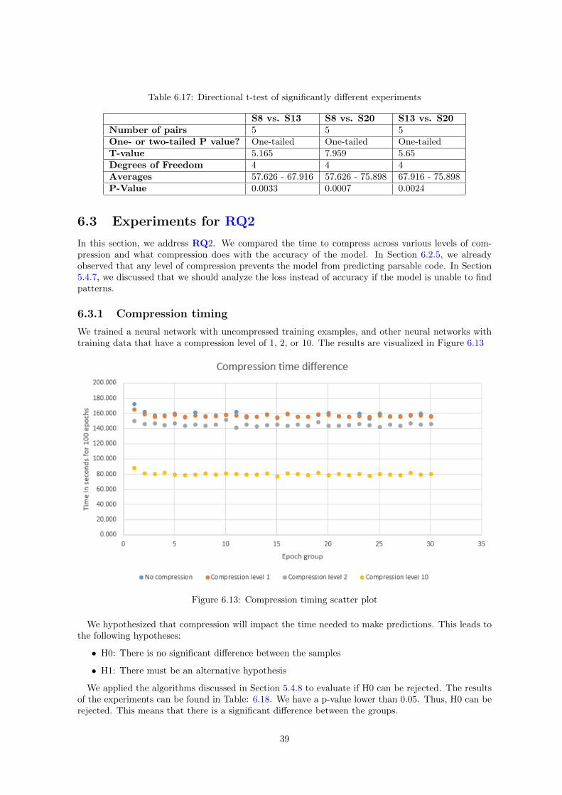
Table 6.17: Directional t-test of significantly different experiments

S8 vs. S13 S8 vs. S20 S13 vs. S20Number of pairs 5 5 5One- or two-tailed P value? One-tailed One-tailed One-tailedT-value 5.165 7.959 5.65Degrees of Freedom 4 4 4Averages 57.626 - 67.916 57.626 - 75.898 67.916 - 75.898P-Value 0.0033 0.0007 0.0024

6.3 Experiments for RQ2

In this section, we address RQ2. We compared the time to compress across various levels of com-pression and what compression does with the accuracy of the model. In Section 6.2.5, we alreadyobserved that any level of compression prevents the model from predicting parsable code. In Section5.4.7, we discussed that we should analyze the loss instead of accuracy if the model is unable to findpatterns.

6.3.1 Compression timing

We trained a neural network with uncompressed training examples, and other neural networks withtraining data that have a compression level of 1, 2, or 10. The results are visualized in Figure 6.13

Figure 6.13: Compression timing scatter plot

We hypothesized that compression will impact the time needed to make predictions. This leads tothe following hypotheses:

• H0: There is no significant difference between the samples

• H1: There must be an alternative hypothesis

We applied the algorithms discussed in Section 5.4.8 to evaluate if H0 can be rejected. The resultsof the experiments can be found in Table: 6.18. We have a p-value lower than 0.05. Thus, H0 can berejected. This means that there is a significant difference between the groups.

39

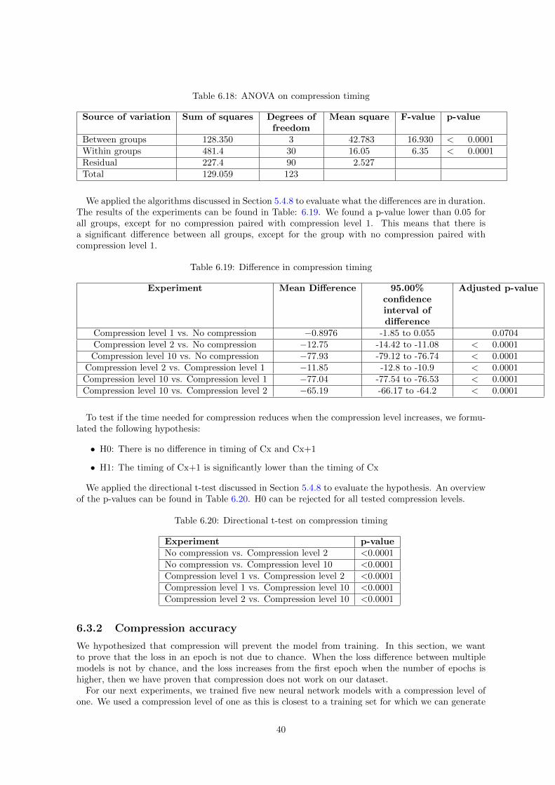
Table 6.18: ANOVA on compression timing

Source of variation Sum of squares Degrees offreedom

Mean square F-value p-value

Between groups 128.350 3 42.783 16.930 < 0.0001Within groups 481.4 30 16.05 6.35 < 0.0001Residual 227.4 90 2.527Total 129.059 123

We applied the algorithms discussed in Section 5.4.8 to evaluate what the differences are in duration.The results of the experiments can be found in Table: 6.19. We found a p-value lower than 0.05 forall groups, except for no compression paired with compression level 1. This means that there isa significant difference between all groups, except for the group with no compression paired withcompression level 1.

Table 6.19: Difference in compression timing

Experiment Mean Difference 95.00%confidenceinterval ofdifference

Adjusted p-value

Compression level 1 vs. No compression −0.8976 -1.85 to 0.055 0.0704Compression level 2 vs. No compression −12.75 -14.42 to -11.08 < 0.0001Compression level 10 vs. No compression −77.93 -79.12 to -76.74 < 0.0001

Compression level 2 vs. Compression level 1 −11.85 -12.8 to -10.9 < 0.0001Compression level 10 vs. Compression level 1 −77.04 -77.54 to -76.53 < 0.0001Compression level 10 vs. Compression level 2 −65.19 -66.17 to -64.2 < 0.0001

To test if the time needed for compression reduces when the compression level increases, we formu-lated the following hypothesis:

• H0: There is no difference in timing of Cx and Cx+1

• H1: The timing of Cx+1 is significantly lower than the timing of Cx

We applied the directional t-test discussed in Section 5.4.8 to evaluate the hypothesis. An overviewof the p-values can be found in Table 6.20. H0 can be rejected for all tested compression levels.

Table 6.20: Directional t-test on compression timing

Experiment p-valueNo compression vs. Compression level 2 <0.0001No compression vs. Compression level 10 <0.0001Compression level 1 vs. Compression level 2 <0.0001Compression level 1 vs. Compression level 10 <0.0001Compression level 2 vs. Compression level 10 <0.0001

6.3.2 Compression accuracy

We hypothesized that compression will prevent the model from training. In this section, we wantto prove that the loss in an epoch is not due to chance. When the loss difference between multiplemodels is not by chance, and the loss increases from the first epoch when the number of epochs ishigher, then we have proven that compression does not work on our dataset.

For our next experiments, we trained five new neural network models with a compression level ofone. We used a compression level of one as this is closest to a training set for which we can generate

40

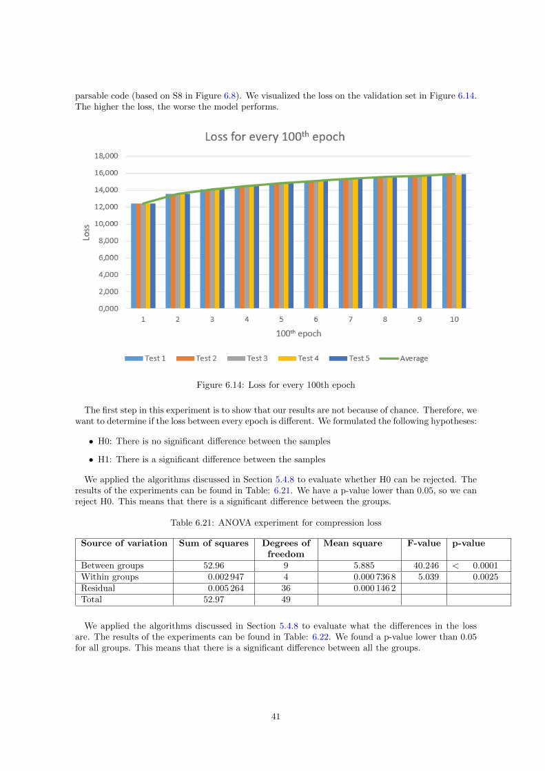
parsable code (based on S8 in Figure 6.8). We visualized the loss on the validation set in Figure 6.14.The higher the loss, the worse the model performs.

Figure 6.14: Loss for every 100th epoch

The first step in this experiment is to show that our results are not because of chance. Therefore, wewant to determine if the loss between every epoch is different. We formulated the following hypotheses:

• H0: There is no significant difference between the samples

• H1: There is a significant difference between the samples

We applied the algorithms discussed in Section 5.4.8 to evaluate whether H0 can be rejected. Theresults of the experiments can be found in Table: 6.21. We have a p-value lower than 0.05, so we canreject H0. This means that there is a significant difference between the groups.

Table 6.21: ANOVA experiment for compression loss

Source of variation Sum of squares Degrees offreedom

Mean square F-value p-value

Between groups 52.96 9 5.885 40.246 < 0.0001Within groups 0.002 947 4 0.000 736 8 5.039 0.0025Residual 0.005 264 36 0.000 146 2Total 52.97 49

We applied the algorithms discussed in Section 5.4.8 to evaluate what the differences in the lossare. The results of the experiments can be found in Table: 6.22. We found a p-value lower than 0.05for all groups. This means that there is a significant difference between all the groups.

41

Table 6.22: Difference in loss groups

Experiment Mean Difference 95.00%confidenceinterval ofdifference

Adjusted p-value

Epoch 200 vs. Epoch 100 1.166 1,132 to 1,201 < 0.0001Epoch 300 vs. Epoch 200 0.5446 0,5224 to 0,5668 < 0.0001Epoch 400 vs. Epoch 300 0.396 0,3729 to 0,4192 < 0.0001Epoch 500 vs. Epoch 400 0.3231 0,3063 to 0,3398 < 0.0001Epoch 600 vs. Epoch 500 0.2656 0,2211 to 0,3101 < 0.0001Epoch 700 vs. Epoch 600 0.2346 0,1818 to 0,2873 0.0002Epoch 800 vs. Epoch 700 0.1964 0,1602 to 0,2325 0.0001Epoch 900 vs. Epoch 800 0.1888 0,1589 to 0,2188 < 0.0001Epoch 1000 vs. Epoch 900 0.1464 0,1017 to 0,191 0.0005

To test if the loss increases, we formulated the following hypothesis:

• H0: There is no significant difference between the loss of Ex and Ex+1

• H1: The loss of Ex+1 is significantly higher than the loss of Ex

We applied the directional t-test discussed in Section 5.4.8 to evaluate the hypothesis. An overviewof the p-values can be found in Table 6.23. We can reject H0 for all compression levels, meaning thatthe loss increases after every epoch.

Table 6.23: Directional t-test on compression loss

Experiment p-valueEpoch 200 vs. Epoch 100 <0.0001Epoch 300 vs. Epoch 200 <0.0001Epoch 400 vs. Epoch 300 <0.0001Epoch 500 vs. Epoch 400 <0.0001Epoch 600 vs. Epoch 500 <0.0001Epoch 700 vs. Epoch 600 <0.0001Epoch 800 vs. Epoch 700 <0.0001Epoch 900 vs. Epoch 800 <0.0001Epoch 1,000 vs. Epoch 900 <0.0001

6.4 Applying SBT in the experiments

In Section 6.2 and 6.3, we trained our models based on a textual representation. However, in thisform, the structure of the grammar is invisible. With SBT, this information can be captured in atextual form so that the neural network can learn the code structure. This could make it easierfor the machine learning algorithm to capture the structure of the code and improve its predictioncapabilities [HWLJ18]. In Section 6.2.6 we mentioned that we applied SBT to our experiments, butthat we could not get any parsable code. This chapter addresses the problems that we encountered.

6.4.1 Output length

Our goal is to translate source code into tests. However, the SBT representations are very long. Whenwe select the 10,000 smallest training examples, we have a maximum token length of 714 comparedto 91 tokens maximum for method code. The problem of a larger sequences is that it increases thememory usage on the GPU. In this case, SBT has 7.85 (714/91) times the size of normal code. Thiscan cause issues during training.

42

Limiting the training examples is not an option. The number of training examples is already lowwhen we compared it to the number of training used in related research mentioned in Section 3.1.3.

6.4.2 Training

To support the sequence length of 714, we could only use a neural network with LSTM nodes of size64 instead of 512. Using LSTM nodes of size 512 was impossible because of memory limitations. Weselected the smallest 9,998 training examples for method code and 9,995 training examples for SBT.We trained a model for both sets with this network setup. We could not generate valid SBT trees. Wewere able to generate parsable method code. However, the generated code did not make any sense.It consists of method bodies that asserted two empty string. The results are inconclusive, because itwas impossible to use a reasonable neural network in combination with SBT.

6.4.3 First steps to a solution

We tried to reduce the AST structure as much as possible by removing redundant layers. For example,in the AST, a NameExpr only has a SimpleName as a child which only has a string as a child. Thismakes the SimpleName in between redundant, so we removed it. With this type of compression, wewere able to reduce the maximum token size of the first 10,000 training example by 20.17% (714 to570). However, this reduction is too small to enable the use of a reasonable size neural network. Itshould at least be possible to use a network of 512 LSTM nodes in the encoder and decoder.

We also tried to use the compression algorithm of Ling et al. [LGH+16]. However, the algorithmwill increase the vocabulary size because there are more repeated token combinations. An overview ofthe compression levels can be found in Table 6.24. This greater vocabulary size increased the memoryneeded to train the model, which made training the model impossible.

Table 6.24: SBT compression effect

Level of compression Vocabulary size Max sequence sizeNone 9,123 570Level 2 176,546 220Level 3 227,575 168Level 4 237,795 144Level 5 222,916 136

43

Chapter 7

Discussion

In this chapter, we discuss our experiment results on i) what neural network solution performs best togenerate unit tests, and ii) how compression affects accuracy and performance. First, we start with asummary of our most important results.

7.1 Summary of the results

We noticed that we could extract more training examples by using an AST analysis instead of abytecode analysis. However, bytecode analysis has still advantages over AST analysis. Only bytecodeanalysis can extract training examples when in the example the base type of the class under test isused. This means even if AST analysis can extract more training examples, bytecode analysis is stillneeded in order to get a dataset that includes examples that use basic object-oriented code.

When we train a neural network, then we see an improvement in the amount of parsable code gener-ated when we only including examples with a sequence length of maximal 100 tokens. Increasing thesequence length more reduces this. There is no improvement noticed when different or a combinationof other optimizations are evaluated. Besides, there was also no improvement when different dataviews are applied. One of the data views was the compressed view. For this view, we saw a reductionof time needed to train models. However, with this view, we were unable to produce parsable code.When we applied SBT, we also could not generate working models. This was since SBT had a largenegative impact on sequence length. This made it impossible for our neural network to train on thisdata. Tuning the neural network configuration improved how much parsable code could be generated.There was an improvement when the number of output layers is set to two instead of one, and whena 50% dropout is configured. We are unable to generate test code, but the increase in the amount ofparsable code could indicate that the neural network is starting to learn how code is written. Writingcode itself is complicated. When we can improve our test generator further, then we could start tosee patterns in the predictions on how code can be tested.

7.2 RQ1: What neural network solutions can be applied togenerate test suites in order to achieve a higher test suiteeffectiveness for software projects?

For this research question, we first addressed the parsable code metrics that we used to measureperformance. This metric is critical in this research, and is used to guide the research towards morepromising solutions. With this metric, we analyzed the results of various models.

7.2.1 The parsable code metric

The application of machine learning to test suite generators is very new. For this research, onlythe generation of parsable code was achieved. Unfortunately, this does not give any insights into

44

how well the code tests. It will give an idea if the machine learning model starts to understand theprogramming language. This is a first step towards generating test code. However, more research onother metrics could give a better insight into the progress towards a unit test generator using machinelearning.

7.2.2 Training on a limited sequence size

A big part of generating more parsable code was filtering training examples. A great improvementwas made when we limited training examples to a sequence length of 100 tokens. The effect of betterpredictions with smaller sequences was also noticed in other research by Bahdanau et al. [BCS+15].We confirm this finding.

7.2.3 Using training examples with common subsequences

During our experiments, we got better results when we only used training examples with commonsubsequences and a sequence length of 100 tokens. Later, it turned out that it did not improve ourresults. The reason why this should have worked is that the neural network can learn context. This isrelated to research into BPE. With BPE, translation scores were improved by linking words that arewritten differently (loving - love) but have (almost) the same meaning [SHB15]. So, including trainingexamples that are related to other training examples should give the neural network the ability tolearn more complex transformations. However, when we only include training examples with a lot ofcontext, we make it harder for the model to make predictions. In addition, the test set also consists oftraining examples with a lot of context. Therefore, a lower score in parsable rate does not necessarilymean that it is worse in predicting test code. Future research could give more insight when a metriccan be applied that is more accurate in the development phase of the test generator.

We performed many experiments on top of this. When this set indeed reduces the ability to writetest code, then this only means that we could have achieved a higher parsable rate. This will notinvalidate any results.

7.2.4 BPE

Applying BPE on our datasets reduced the amount of parsable code that could be generated. Weused BPE to include relations between words and symbols instead of word part. Other research foundthat in NLP the addition of the relation between word part improves results [SHB15]. A reason whythis does not work on words in code could be because there are too many relations that make nosense. For example, because of BPE, the word stop in both stopSign and stopWalking share some levelof meaning. These two identifiers do not have much in common when translating to code. This couldbe the reason why we observed a drop in the percentage of generated parsable code. However, we didnot perform a statistical check to validate these results.

7.2.5 Network configuration of related research

During the experiments, we have tried various network configurations. One configuration we triedwas similar to the network used by Hu et al. [HWLJ18], which they used to summarize code. Thisconfiguration did not work with our experiments, because they used a too high learning rate for ourdata. With a higher learning rate, less time is needed to create the model, since great steps are takenduring the learning process. A high learning rate could mean that it never reaches the ideal model.However, our model did not learn anything. We expect that our data is harder to generalize, soadjusting each training step too much will cause the modifications to be too specific.

7.2.6 SBT

We were unable to use SBT to generate code, since it outputs sequences which are too long. We wereunable to reduce the sequences to a level where we can train a sufficient neural network. Also, wecould not compress the sequences too much, because the whole point is to add additional information.

45

When we compress it too much, we lose this information. In future research, other machine learningsolutions could be applied which are capable of handling this kind of data. For instance, instead oftranslating based on words, translations could be done based on sections [HWZD17].

7.2.7 Comparing our models

In Section 6.2, we observed big differences between experiments. In Section 6.2.8, we did not find astatistical correlation between all these experiments. There still could be a correlation, but it wasnot noticeable. This could be caused by a too small sample size. An overview of all experimentscan be found in Figure 6.12. Table 6.17 shows that the result of S20 is better than S8 and S13, andthe result of S13 is better than S8. From these relations, we can conclude that on our dataset S8we have better results when we use one input layer and two output layers instead of one input layerand one output layer. In addition, by adding a dropout of 50% to this configuration will improve theresults further. The reason for the improved results is that, when adding another output layer and50% dropout, the network now can make more advanced conclusions and the network can make moreindependent decisions. The first layer can capture the general conclusion and the second layer canmake more advance conclusions based on the previous conclusions.

7.3 RQ2: What is the impact of input and output sequencecompression on the training time and accuracy?

Compression can make the application of the used machine learning technique easier, because one ofthe weak points of our technique is long sequence lengths. Compression could improve the resultsby solving this problem and reduces the time needed to train models. For compression, we used thealgorithm proposed by Ling et al. [LGH+16].

7.3.1 Training time reduction

We noticed an improvement when applying the compression to the input and output sequences.Unfortunately, Ling et al. [LGH+16] did not report on the time reduction of the training time of theirmodels. However, we found a significant time reduction on our dataset.

7.3.2 Increasing loss

In the experiments for RQ1, we observed that we were unable to generate parsable code with com-pression. We expected that, with compression, too much information is captured in a single token.This could make predicting code harder, as every token has too much meaning. We also noticed thatduring training the loss increases on the validation set. This increase means that the neural networkfailed to learn patterns. These issues contradict the research done by Ling et al. [LGH+16]. However,we were unable to generate test code without compression. Ling et al. [LGH+16] managed to gener-ate working code without applying compression. Therefore, it could be that compression only workswhen the neural network can capture the problem. The problem why we cannot generate workingcode could be caused by our dataset, because the dataset may exist out of barely related trainingexamples. Compression could make them even more unrelated, what could have a negative impact.When the training set would have contained training examples that are very related, then reducingthis could give only a small penalty. The positive impact of compression (reducing sequence length)could be greater than the penalty of making the training examples more unrelated.

7.4 Limitations

The scope of this project is to find out if neural networks can be used for unit test generation. Westill left many questions and problems unanswered, of which some are listed in this chapter.

46

7.4.1 The used mutation testing tool

To calculate the mutation score of our baseline, we used an alternative version of PIT MutationTesting to calculate the mutation testing score. During our study, this tool achieved the most reliableresult to measure test suite effectiveness. However, new versions of the original tool were released andcould outperform this version. The mutation generation ability of the original tool should be checkedin future research and used when it performs better. Our research is not invalid when the originaltool performs better, because we did not perform comparisons on the baseline yet. Even if we did, itwould not have made a difference. The result should only be more accurate when comparing to realfaults.

7.4.2 JUnit version

During the start of the project, Junit 4 was the latest version of this test framework. However, duringthe project Junit 5 was released [Junc]. We did not restart our gathering process, because a recentlyreleased version will be used by fewer projects than a version which has been around for 12 years[Junb].

7.4.3 More links for AST analysis depends on data

We noticed that for our research AST analysis could create more links than bytecode analysis, becauseit supports more projects. We did not perform a statistical check to validate this, because it was notof importance whether one method was better compared to another. More in-depth research shouldbe performed when these techniques are compared in future research.

7.4.4 False positive links

In section 6.1.3, we mentioned the number of links we could create on a set of projects. However, itis possible that for some tests an incorrect class under test is used. This could have resulted in falsepositive matches. Many of them could be eliminated with backward slicing, as described in section3.2.1. We expect that most false positives are eliminated when we link based on the statementsreturned by this method.

7.5 The dataset has an impact on the test generators quality

In our research, we only considered a selection of open-source projects. The result could be differentwhen other open or closed-source projects were used.

7.5.1 Generation calls to non-existing methods

The unit tests in our training examples use helper functions developed for the tests, while we donot include these in the training data. Thus, our generated tests will contain calls to non-existingmethods. We limited our research by not looking into this problem. Support for these cases has tobe addressed in further research.

7.5.2 Testing a complete method

In an average software project, multiple unit tests exist for a single method. Every unit test is writtenfor a small part of the method code. We did not embed this relation in our dataset. Therefore,our machine learning model has to learn this relation on its own. It has to learn from the trainingdata that some parts of the method translate to a single unit test. In future research, a more directtranslation should be performed because it makes learning easier. It will be easier since this will limitthe sequence length and will relieve the machine learning algorithm from unnecessary complexity.

47

7.5.3 The machine learning model is unaware of implementations

During training, the machine learning model learns the usage of many methods. When the modelis applied for making predictions on unseen data, it will see new method calls which it has notencountered before. The model could know what the call does based on its naming and context.However, it would be easier for the machine learning algorithm to have more detailed informationsuch as the implementation of the method. Thus, the information in our training examples is limited.Adding more detail could make predictions easier.

7.5.4 Too less data for statistical proving our models

In most of our statistical analysis, we used five samples per group. In future research, the sample sizeshould be increased to validate our findings.

7.5.5 Replacing manual testing

A potential risk is introduced when our method is replacing humans for writing tests. Our generatorcould be unable to cover all mutants that would have been captured by a human. This will result inless test suites effectiveness.

48

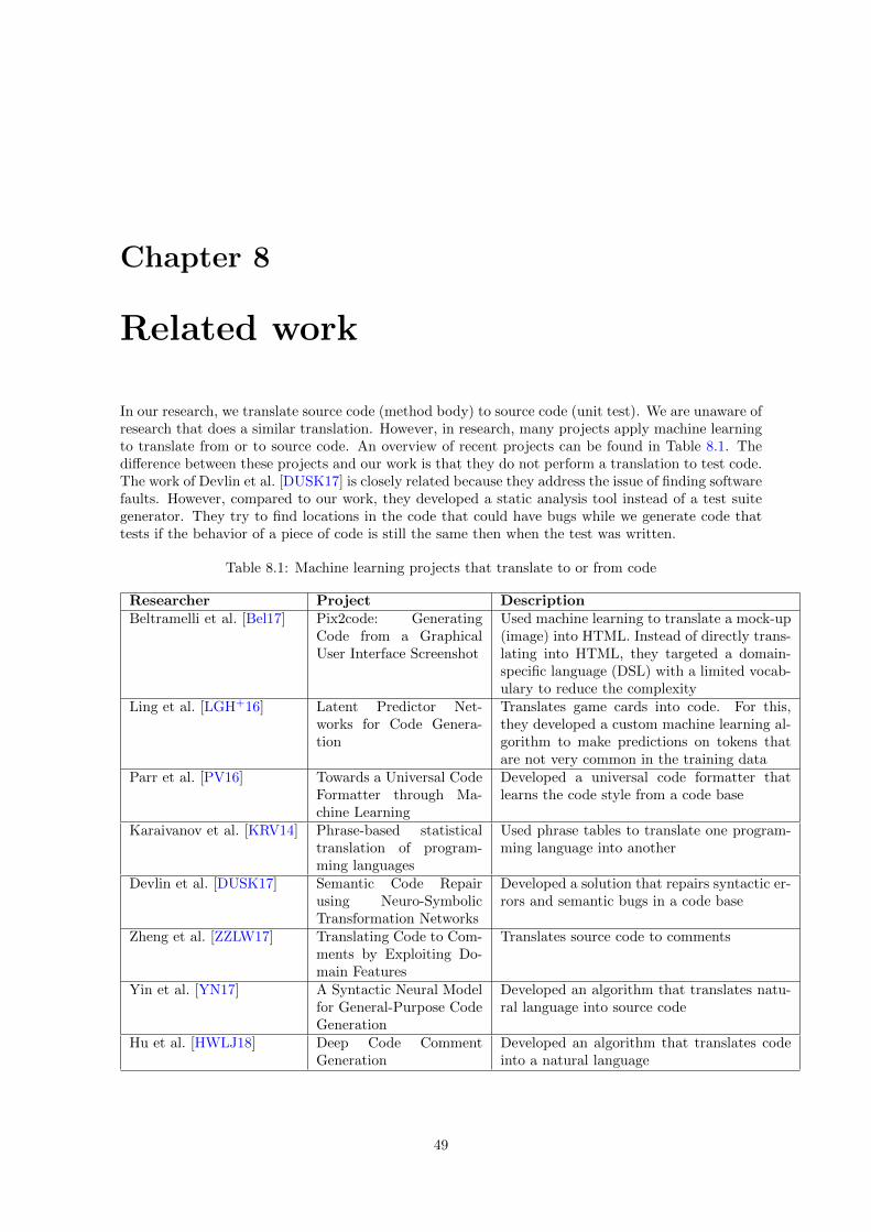
Chapter 8

Related work

In our research, we translate source code (method body) to source code (unit test). We are unaware ofresearch that does a similar translation. However, in research, many projects apply machine learningto translate from or to source code. An overview of recent projects can be found in Table 8.1. Thedifference between these projects and our work is that they do not perform a translation to test code.The work of Devlin et al. [DUSK17] is closely related because they address the issue of finding softwarefaults. However, compared to our work, they developed a static analysis tool instead of a test suitegenerator. They try to find locations in the code that could have bugs while we generate code thattests if the behavior of a piece of code is still the same then when the test was written.

Table 8.1: Machine learning projects that translate to or from code

Researcher Project DescriptionBeltramelli et al. [Bel17] Pix2code: Generating

Code from a GraphicalUser Interface Screenshot

Used machine learning to translate a mock-up(image) into HTML. Instead of directly trans-lating into HTML, they targeted a domain-specific language (DSL) with a limited vocab-ulary to reduce the complexity

Ling et al. [LGH+16] Latent Predictor Net-works for Code Genera-tion

Translates game cards into code. For this,they developed a custom machine learning al-gorithm to make predictions on tokens thatare not very common in the training data

Parr et al. [PV16] Towards a Universal CodeFormatter through Ma-chine Learning

Developed a universal code formatter thatlearns the code style from a code base

Karaivanov et al. [KRV14] Phrase-based statisticaltranslation of program-ming languages

Used phrase tables to translate one program-ming language into another

Devlin et al. [DUSK17] Semantic Code Repairusing Neuro-SymbolicTransformation Networks

Developed a solution that repairs syntactic er-rors and semantic bugs in a code base

Zheng et al. [ZZLW17] Translating Code to Com-ments by Exploiting Do-main Features

Translates source code to comments

Yin et al. [YN17] A Syntactic Neural Modelfor General-Purpose CodeGeneration

Developed an algorithm that translates natu-ral language into source code

Hu et al. [HWLJ18] Deep Code CommentGeneration

Developed an algorithm that translates codeinto a natural language

49

Chapter 9

Conclusion

Incorporating machine learning in a test generator could lead to better test generation. A generatorlike this cannot only be used to generate a complete test suite; it can also be used to aid softwareengineers in writing tests. Nevertheless, more work has to be done to get to this point.

To our knowledge, this research is the first study towards test generation with the application ofmachine learning. We were able to create a training set for this problem, and managed to trainneural networks with this dataset. We extracted more than 52,000 training examples from 1,106software projects. When training machine learning models, we noticed that the quality of our modelsimproved when configurations are tweaked and when the training data was filtered. Our first resultsare promising, and we see many opportunities to continue the development of the test generator. Webelieve that our results could be further improved when a machine learning algorithm specific for codetranslation is used, if the neural network is trained on how small parts of the code are tested insteadof whole methods, and when the neural network has more detailed implementation information. Ourresults can be used as a baseline for future research.

We also experimented with machine learning approaches that improved the results of other studies.We applied compression, SBT, and BPE on our training set. A correlation was found that indicatesthat the time needed to train a model is reduced when compression is applied. An improved com-pression algorithm or a dataset optimized for the compression technique could be used to create amodel that can make good predictions in less time, what will make research in this field more efficient.We also improved the application of SBT in translations to code. We developed an algorithm thatcan translate an SBT representation back to code (Appendix A). This tool could already be used forexperiments when the output length is limited. BPE was also applied, to let our model use additionalinformation on how parts of the training data are connected. In our experiment, it did not have apositive effect. However, optimizing the number of connections could work for our datasets when onlyconnections that add relevant information are included.

All steps from finding suitable GitHub projects until the calculation of the parsable score areautomated in scripts. A copy can be found in Appendix A. With these scripts, all results of ourexperiments can be reproduced. The first part of the scripts can be executed to retrieve trainingexamples or the provided backups with the used training examples can be restored. When it ispreferred to download all projects, then the overview of all used repositories should be used. Weincluded the used commits in the GitHub links. The second part is to configure the dataset generatoraccording to the parameters in our experiments. From this point, the rest of the scripts can be usedto execute the rest of the pipeline in order to calculate the parsable score.

To summarize, with this research we contribute an algorithm that can be used to generate trainingexamples (for method to test translations), the training sets used in our experiments, SBT to codeimplementation, and a neural network configuration that can learn basic patterns between methodsand test code. Finally, we also contribute software that takes GitHub repositories as input and amodel that can be used to predict tests with machine learning as output.

50

Chapter 10

Future work

There are still some additional experiments which could add value to the presented work. We did notmanage to do experiments with SBT, and we did not investigate further if the percentage of commonsubsequences has an impact on the results of the neural network. Additionally, we found some areasthat are promising for a machine learning based test generator that we did not address.

10.1 SBT and BPE

Both BPE and SBT did not positively affect our results. We could not generate valid trees withSBT because of hardware/software limitations. The concept of SBT is very promising and should beaddressed in future research. BPE was also applied on our training data. In future research, it shouldbe tested if optimizing the number of connections improves results by only introducing a connectionthat adds relevant information.

10.2 Common subsequences

We performed experiments where we filtered training examples based on the level of common subse-quences. We only kept training examples where more than 80% of the training example are commonunder other training examples. An optimized percentage could result in better predictions. In futureresearch, the rate of common subsequences could be tuned to find out what the effect of varying thepercentage is.

10.2.1 Filtering code complexity with other algorithms

During our research, we filtered complex training examples (Section 6.2.2). We only checked if concreteclasses and default methods were used. However, more criteria could be tested. For instance, trainingexamples that have a too high cyclomatic complexity could be excluded.

10.3 Promising areas

Apart from future work, there are many areas that we did not address in our research while theyhave the potential to improve our results. The time needed to train models could be reduced toallow future research to train more models in the same amount of time and have a shorter feedbackloop. Additionally, an optimized machine learning algorithm could be developed for code-to-codeconversion.

10.3.1 Reducing the time required to train models

To find out if a change in the machine learning configuration had a positive or negative impact on ourresults, we had to wait for 12-24 hours. This time could be reduced when a mechanism is incorporated

51

that can eliminate predictions when they are only partially processed. Predictions could be eliminatedwhen they are not compliant with the language’s grammar. This could have a positive impact sincemodels are applied to the validation set during training.

10.3.2 Optimized machine learning algorithm

To our knowledge, there are no machine learning algorithms that target code-to-code translations. Analgorithm could be developed that is specialized in these code-to-code problems. This algorithm couldbe used by the unit test generator, while it could also be used for other general translation problems.The algorithm target the challenges that we encountered during our research. For example, thedifficulty to make predictions over a long sequence length, and the difficulty to learn code structure.

52

Bibliography

[Abd10] Herve Abdi. The greenhouse-geisser correction. Encyclopedia of research design, 1:544–548, 2010.

[AHF+17] M Moein Almasi, Hadi Hemmati, Gordon Fraser, Andrea Arcuri, and Janis Benefelds.An industrial evaluation of unit test generation: Finding real faults in a financial ap-plication. In Proceedings of the 39th International Conference on Software Engineering:Software Engineering in Practice Track, 2017.

[APS16] Miltiadis Allamanis, Hao Peng, and Charles Sutton. A convolutional attention networkfor extreme summarization of source code. In International Conference on MachineLearning, 2016.

[BCB14] Dzmitry Bahdanau, Kyunghyun Cho, and Yoshua Bengio. Neural machine translationby jointly learning to align and translate. CoRR, abs/1409.0473, 2014. URL: http://arxiv.org/abs/1409.0473, arXiv:1409.0473.

[BCS+15] Dzmitry Bahdanau, Jan Chorowski, Dmitriy Serdyuk, Philemon Brakel, and YoshuaBengio. End-to-end attention-based large vocabulary speech recognition. CoRR,abs/1508.04395, 2015. URL: http://arxiv.org/abs/1508.04395, arXiv:1508.04395.

[BdCHP10] Jose Bernardo Barros, Daniela da Cruz, Pedro Rangel Henriques, and Jorge SousaPinto. Assertion-based slicing and slice graphs. In Proceedings of the 2010 8thIEEE International Conference on Software Engineering and Formal Methods, SEFM’10, pages 93–102, Washington, DC, USA, 2010. IEEE Computer Society. URL:http://dx.doi.org/10.1109/SEFM.2010.18, doi:10.1109/SEFM.2010.18.

[Bel17] Tony Beltramelli. pix2code: Generating code from a graphical user interface screen-shot. CoRR, abs/1705.07962, 2017. URL: http://arxiv.org/abs/1705.07962, arXiv:1705.07962.

[CDE+08] Cristian Cadar, Daniel Dunbar, Dawson R Engler, et al. Klee: Unassisted and automaticgeneration of high-coverage tests for complex systems programs. In OSDI, volume 8,pages 209–224, 2008.

[CGCB14] Junyoung Chung, Caglar Gulcehre, KyungHyun Cho, and Yoshua Bengio. Empir-ical evaluation of gated recurrent neural networks on sequence modeling. CoRR,abs/1412.3555, 2014. URL: http://arxiv.org/abs/1412.3555, arXiv:1412.3555.

[CVMG+14] Kyunghyun Cho, Bart Van Merrienboer, Caglar Gulcehre, Dzmitry Bahdanau, FethiBougares, Holger Schwenk, and Yoshua Bengio. Learning phrase representations usingrnn encoder-decoder for statistical machine translation. arXiv preprint arXiv:1406.1078,2014.

[DUSK17] Jacob Devlin, Jonathan Uesato, Rishabh Singh, and Pushmeet Kohli. Semantic coderepair using neuro-symbolic transformation networks. CoRR, abs/1710.11054, 2017.arXiv:1710.11054.

53

[FRCA17] Gordon Fraser, Jose Miguel Rojas, Jose Campos, and Andrea Arcuri. Evosuite atthe sbst 2017 tool competition. In Proceedings of the 10th International Workshop onSearch-Based Software Testing, 2017.

[FZ12] Gordon Fraser and Andreas Zeller. Mutation-driven generation of unit tests and oracles.IEEE Transactions on Software Engineering, 38(2), 2012.

[GAG+17] Jonas Gehring, Michael Auli, David Grangier, Denis Yarats, and Yann N. Dauphin.Convolutional sequence to sequence learning. CoRR, abs/1705.03122, 2017. URL: http://arxiv.org/abs/1705.03122, arXiv:1705.03122.

[Git] Github. Rest api v3 search. https://developer.github.com/v3/search/. Accessed:2018-06-04.

[HWLJ18] Xing Hu, Yuhan Wei, Ge Li, and Zhi Jin. Deep code comment generation. ICPC 2018,2018.

[HWZD17] Po-Sen Huang, Chong Wang, Dengyong Zhou, and Li Deng. Neural phrase-based ma-chine translation. CoRR, abs/1706.05565, 2017. URL: http://arxiv.org/abs/1706.05565, arXiv:1706.05565.

[JJI+14] Rene Just, Darioush Jalali, Laura Inozemtseva, Michael D Ernst, Reid Holmes, andGordon Fraser. Are mutants a valid substitute for real faults in software testing? InProceedings of the 22nd ACM SIGSOFT International Symposium on Foundations ofSoftware Engineering, 2014.

[Juna] Junit. Junit 4 download and install. https://github.com/junit-team/junit4/wiki/Download-and-Install. Accessed: 2018-06-04.

[Junb] Junit. Junit 4 release notes. https://sourceforge.net/projects/junit/files/

junit/4.0/. Accessed: 2018-06-04.

[Junc] Junit. Junit 5 release notes. https://junit.org/junit5/docs/snapshot/

release-notes/. Accessed: 2018-06-04.

[KC17] Timotej Kapus and Cristian Cadar. Automatic testing of symbolic execution enginesvia program generation and differential testing. In Proceedings of the 32nd IEEE/ACMInternational Conference on Automated Software Engineering, 2017.

[KRV14] Svetoslav Karaivanov, Veselin Raychev, and Martin Vechev. Phrase-based statisticaltranslation of programming languages. In Proceedings of the 2014 ACM InternationalSymposium on New Ideas, New Paradigms, and Reflections on Programming & Software,2014.

[LGH+16] Wang Ling, Edward Grefenstette, Karl Moritz Hermann, Tomas Kocisky, AndrewSenior, Fumin Wang, and Phil Blunsom. Latent predictor networks for code gen-eration. CoRR, abs/1603.06744, 2016. URL: http://arxiv.org/abs/1603.06744,arXiv:1603.06744.

[LKT09] Hui Liu and Hee Beng Kuan Tan. Covering code behavior on input validation in func-tional testing. Inf. Softw. Technol., 51(2):546–553, February 2009. URL: http://dx.doi.org/10.1016/j.infsof.2008.07.001, doi:10.1016/j.infsof.2008.07.001.

[Maa97] Wolfgang Maass. Networks of spiking neurons: the third generation of neural networkmodels. Neural networks, 10(9):1659–1671, 1997.

[MB89] Keith E Muller and Curtis N Barton. Approximate power for repeated-measures anovalacking sphericity. Journal of the American Statistical Association, 84(406):549–555,1989.

54

[ND12] Srinivas Nidhra and Jagruthi Dondeti. Black box and white box testing techniques-aliterature review. International Journal of Embedded Systems and Applications (IJESA),2(2):29–50, 2012.

[Ost02a] Thomas Ostrand. Black-box testing. Encyclopedia of Software Engineering, 2002.

[Ost02b] Thomas Ostrand. White-box testing. Encyclopedia of Software Engineering, 2002.

[PM17] Annibale Panichella and Urko Rueda Molina. Java unit testing tool competition-fifthround. In IEEE/ACM 10th International Workshop on Search-Based Software Testing(SBST), 2017.

[PMm17] Van Beckhoven P, Oprescu A M, and Bruntink m. Assessing test suite effectiveness usingstatic metrics. 10th Seminar on Advanced Techniques and Tools for Software Evolution,2017.

[Poi] Yolande Poirier. What are the most popular libraries java developersuse? based on github’s top projects. https://blogs.oracle.com/java/

top-java-libraries-on-github. Accessed: 2018-06-04.

[PV16] Terence Parr and Jurgen J. Vinju. Technical report: Towards a universal code formatterthrough machine learning. CoRR, abs/1606.08866, 2016. arXiv:1606.08866.

[REP+11] Brian Robinson, Michael D Ernst, Jeff H Perkins, Vinay Augustine, and Nuo Li. Scalingup automated test generation: Automatically generating maintainable regression unittests for programs. In Proceedings of the 26th IEEE/ACM International Conference onAutomated Software Engineering, 2011.

[SHB15] Rico Sennrich, Barry Haddow, and Alexandra Birch. Neural machine translation of rarewords with subword units. CoRR, abs/1508.07909, 2015. URL: http://arxiv.org/abs/1508.07909, arXiv:1508.07909.

[SSN12] Martin Sundermeyer, Ralf Schluter, and Hermann Ney. Lstm neural networks for lan-guage modeling. In Thirteenth Annual Conference of the International Speech Commu-nication Association, 2012.

[SVL14] Ilya Sutskever, Oriol Vinyals, and Quoc V Le. Sequence to sequence learning with neuralnetworks. In Advances in neural information processing systems, 2014.

[VSP+17] Ashish Vaswani, Noam Shazeer, Niki Parmar, Jakob Uszkoreit, Llion Jones, Aidan NGomez, Lukasz Kaiser, and Illia Polosukhin. Attention is all you need. In Advances inNeural Information Processing Systems, pages 6000–6010, 2017.

[YKYS17a] Wenpeng Yin, Katharina Kann, Mo Yu, and Hinrich Schutze. Comparative study ofcnn and rnn for natural language processing. arXiv preprint arXiv:1702.01923, 2017.

[YKYS17b] Wenpeng Yin, Katharina Kann, Mo Yu, and Hinrich Schutze. Comparative study ofCNN and RNN for natural language processing. CoRR, abs/1702.01923, 2017. URL:http://arxiv.org/abs/1702.01923, arXiv:1702.01923.

[YN17] Pengcheng Yin and Graham Neubig. A syntactic neural model for general-purpose codegeneration. CoRR, abs/1704.01696, 2017. URL: http://arxiv.org/abs/1704.01696,arXiv:1704.01696.

[ZM15] Yucheng Zhang and Ali Mesbah. Assertions are strongly correlated with test suiteeffectiveness. In Proceedings of the 10th Joint Meeting on Foundations of SoftwareEngineering, 2015.

[ZZLW17] Wenhao Zheng, Hong-Yu Zhou, Ming Li, and Jianxin Wu. Code attention: Translatingcode to comments by exploiting domain features. CoRR, abs/1709.07642, 2017. arXiv:1709.07642.

55

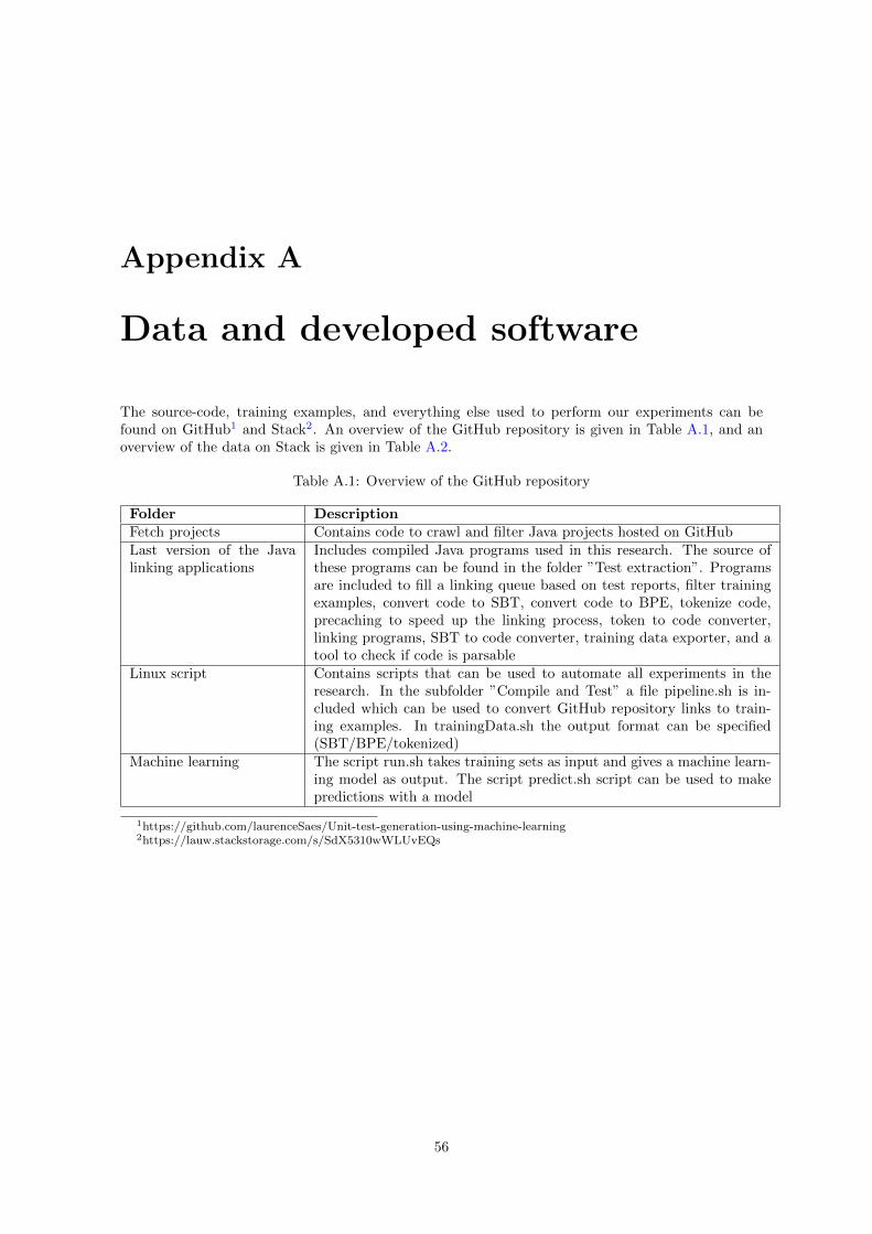
Appendix A

Data and developed software

The source-code, training examples, and everything else used to perform our experiments can befound on GitHub1 and Stack2. An overview of the GitHub repository is given in Table A.1, and anoverview of the data on Stack is given in Table A.2.

Table A.1: Overview of the GitHub repository

Folder DescriptionFetch projects Contains code to crawl and filter Java projects hosted on GitHubLast version of the Javalinking applications

Includes compiled Java programs used in this research. The source ofthese programs can be found in the folder ”Test extraction”. Programsare included to fill a linking queue based on test reports, filter trainingexamples, convert code to SBT, convert code to BPE, tokenize code,precaching to speed up the linking process, token to code converter,linking programs, SBT to code converter, training data exporter, and atool to check if code is parsable

Linux script Contains scripts that can be used to automate all experiments in theresearch. In the subfolder ”Compile and Test” a file pipeline.sh is in-cluded which can be used to convert GitHub repository links to train-ing examples. In trainingData.sh the output format can be specified(SBT/BPE/tokenized)

Machine learning The script run.sh takes training sets as input and gives a machine learn-ing model as output. The script predict.sh script can be used to makepredictions with a model

1https://github.com/laurenceSaes/Unit-test-generation-using-machine-learning2https://lauw.stackstorage.com/s/SdX5310wWLUvEQs

56

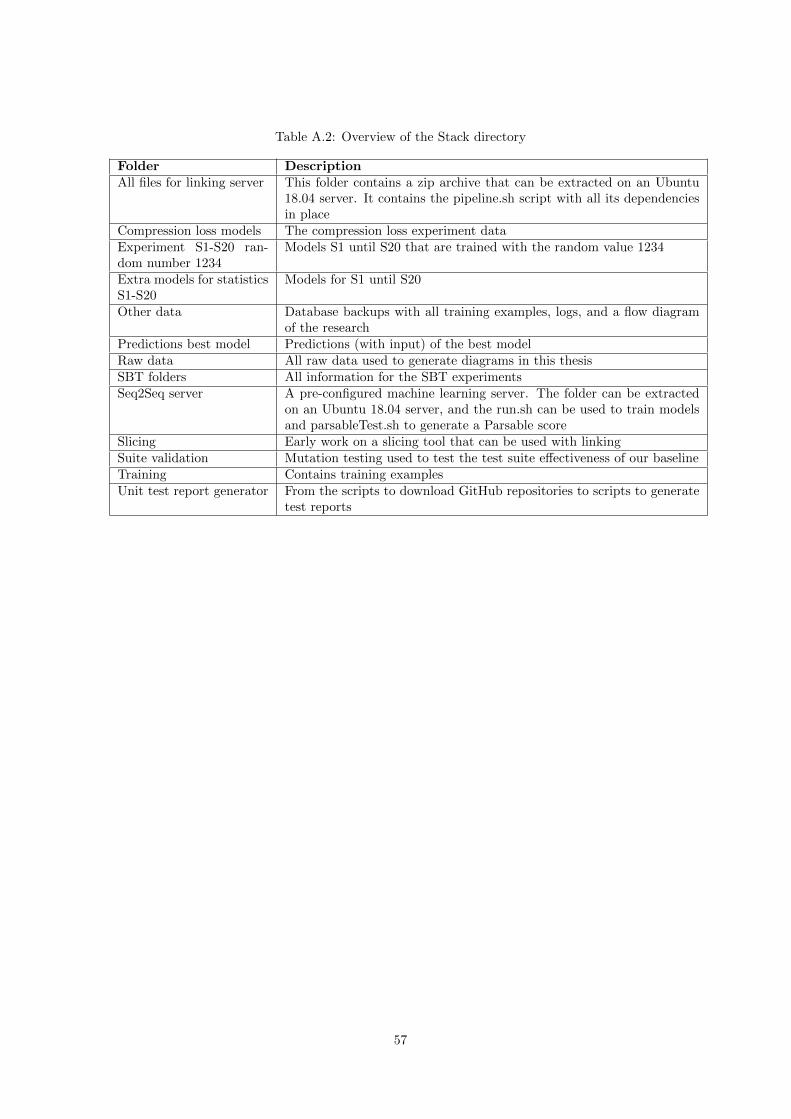
Table A.2: Overview of the Stack directory

Folder DescriptionAll files for linking server This folder contains a zip archive that can be extracted on an Ubuntu

18.04 server. It contains the pipeline.sh script with all its dependenciesin place

Compression loss models The compression loss experiment dataExperiment S1-S20 ran-dom number 1234

Models S1 until S20 that are trained with the random value 1234

Extra models for statisticsS1-S20

Models for S1 until S20

Other data Database backups with all training examples, logs, and a flow diagramof the research

Predictions best model Predictions (with input) of the best modelRaw data All raw data used to generate diagrams in this thesisSBT folders All information for the SBT experimentsSeq2Seq server A pre-configured machine learning server. The folder can be extracted

on an Ubuntu 18.04 server, and the run.sh can be used to train modelsand parsableTest.sh to generate a Parsable score

Slicing Early work on a slicing tool that can be used with linkingSuite validation Mutation testing used to test the test suite effectiveness of our baselineTraining Contains training examplesUnit test report generator From the scripts to download GitHub repositories to scripts to generate

test reports

57