UNIT CONVERSION TABLE

To convert from To Multiply by

inch centimeter 2.54

square inch square centimeter 6.4516

kip kiloNewton (kN) 4.44747

kip/sq. in. (ksi) kN/sq. m (kPa) 6,894.28

ki f t-T kN-meter 1.3556

DISCLAIMER

The opinions, findings and conclusions expressed in this publication are those of the authors who

are responsible for the facts and accuracy of the data presented herein. The contents do not

necessarily reflect the views or the policies of the Florida Department of Transportation or the

Federal Highway Administration. This report does not constitute a standard, specification or

regulation.

The report is prepared in cooperation with the Florida Department of Transportation and the

Federal Highway Administration.

ii

ACKNOWLEDGMENTS

The authors wish to express their sincere thanks to Dr. Mohsen A. Shahawy, Chief Structures

Analyst, and Mr. Adman, Research Engineer, Florida Department of Transportation, for their

excellent suggestions, discussions and constructive criticisms throughout the project. They wish to

express their appreciation to Dr. S. E. Dunn, Professor and Chairman, Department of Ocean

Engineering, and Dr. J. Juvenwicz, Acting Dean, College of Engineering, Florida Atlantic

University for their continued interest and encouragement.

The valuable assistance in the preparation of the report from Mr. Nathaniel Bell and Mrs. Tian

Xang Graduate Students Florida Atlantic University is gratefully acknowledged

iii

SUMMARY

The primary aim of the study was to investigate the wheel load distribution of different bridge types

- solid slab bridges and slab-on-girder bridges with varying skew angles and multiple continuous spans.

The study reviewed the existing analytical and field load distribution methods for different bridge types.

Finite element method was used to carry out the detailed analyses to study the various parameters

affecting wheel load distribution. The data from field tests were collected and analyzed to evaluate the

LRFD specifications and the results from the finite element method.

The influence of the parameters such as skew angle, girder spacing, span length, slab thickness, and

number of traffic lanes was studied in the load distribution of the skew solid slab and skew slab-on-girder

bridges. In addition to the parametric study, data from field tests performed by the Structures Research

Center, FDOT, are compared with those based on FEM analysis, AASHTO and LRFD codes. Simplified

formulae for the effective width of skew solid slab bridges are proposed in this study.

The response of continuous bridges were studied by modeling several continuous bridge types (skew and straight slab-on-girder) using finite element method. Several parameters such as span length, number of spans, ratio between spans and skew angle were considered in the parametric studies. The wheel-load distribution factors from the analyses were compared with the field test data. The study indicated that the analytical results based on finite element method are close to the field test data.

iv

viii

CHAPTER I

INTRODUCTION

1.1 INTRODUCTION

Wheel load distribution on highway bridges is an important response parameter in

determining structural member size and consequently the strength and serviceability of bridge members.

It is, therefore, of critical importance in the design of new bridges and the evaluation of the load carrying

capacity of existing bridges.

The American Association of State Highways and Transportation Officials (AASHTO) method

of load distribution reduces the complex analysis of a bridge subjected to one or more vehicles to simple

analysis of a beam. According to the AASHTO method, the maximum load effects in a girder can be

obtained by treating a girder as a one-dimensional beam subject to loading, which is obtained by

multiplying one line of wheels of the design vehicle by a load fraction (Wheel-Load Distribution Factor).

This concept was first introduced by Newmark (1948).

Recent research resulted in a substantial amount of information on various bridge types

indicating a need for revisions of the AASHTO bridge specifications (1992). These conservative load

distribution factors may be acceptable for the design of new bridges, but are unacceptable for evaluating

1-1

existing bridges. NCHRP project 12-26 (1992) was initiated in the mid-1980s in order to develop

comprehensive specification provisions for distribution of wheel loads in highway bridges.

Within a time span of more than thirty years, the science of bridge analysis and design has undergone major

changes. Following the advent of digital computers, the bridge engineers have available today a number of

powerful analytical tools for refined methods of analysis including (i) the grillage analogy method, (ii) the

orthotropic plate method, (iii) the articulated plate method, and (iv) the finite element method including

finite strip formulation. The results from the above refined methods of analysis should be used to improve

the existing simplified approaches. These approaches would aid the designer to compute the distribution

factors more efficiently without the need for performing complicated analysis in the design office.

Field load testing of highway bridges has increased significantly in recent years. The increased interest has

resulted in part from the large number of older bridges with posted load limits that are below the normal

legal truck weights. Field load testing in determining the safe load capacity of a bridge, which should be

greater than the capacity determined from standard rating calculations based on the AASHTO method. One

method for use of bridge test results in rating calculations is to determine wheel-load distribution factors for

the girders based on test data. These measured wheel-load distribution factors can be used in bridge rating

calculations in the place of those factors defined by AASHTO code.

The studies carried out by the Principal Investigator (Arockiasamy, 1994) on "Load Distribution on

Highway Bridges Based on Field Test Data - Phase I" present the load distribution on certain bridge types

in Florida viz., slab-on-girder, solid slab, voided slab and double-tee bridges. The existing analytical

22-2

and field load distribution methods for different bridge types are reviewed in this study. Grillage analogy

is used as an analytical tool to study the various parameters affecting wheel-load distribution. The results

from the analytical study is compared with those based on the field test data.

1.2 METHODOLOGY AND APPROACH

The finite element method was used to carry out the detailed analyses of different bridge types

- solid slab bridges and slab-on-girder bridges with varying skew angles and multiple continuous spans.

The actual loads used in the bridge tests were modeled in the analysis. The field test results were

compared with the analytical values.

Important parameters such as beam spacing, span length, slab thickness, number of spans,

skew angle, etc. were identified for every bridge type. The average properties were used in the parametric

studies of different bridge types. The data from field tests were collected and analyzed to evaluate

the current LRFD specifications and the results from the finite element method. The structural analysis

program ANSYS was used in the modeling and detailed analysis of different bridge types.

1.2.1 SKEW BRIDGES

The AASHTO specifications (1992) do not include approximate formulae for moments to

account for the effect of skewed supports. It is frequently considered safe to ignore the skew angle, if it

is less than 20 degrees and analyze the bridge as a right bridge with a span equal to the skew span, since

1-23

leads to a conservative safe estimate of longitudinal moments and shears in the skew bridge. The use of

this approximate procedure may lead to significant differences between the skew bridge responses and

those of the equivalent right bridge with larger skew angles.

The influence of the parameters such as girder spacing, span length, slab thickness, flexural

rigidities of longitudinal and transverse girders, number of traffic lanes and total curb-to-curb deck width

were studied in the load distribution of the skew bridges for varying skew angles. The available field test

data for different skew bridge types viz., solid slab and slab-on-AASHTO girder, etc. were analyzed and

compared with the analytical results.

1.2.2 CONTINUOUS BRIDGES

The response of continuous bridges were studied by modeling several continuous bridge

types (slab bridges, beam-and-slab bridges, etc.) using finite element method. The wheel-load distribution

factors from the analyses were compared with the field test data.

1.3 OBJECTIVES AND SCOPE

The objective of the research in Phase II is to determine the load distribution factors for the

following specific bridge types:

(I) Slab-on-bulb-Tee girder bridges

1-24

(iii) Continuous bridges

The load distribution parametric studies were carried out using finite element method. The measured field

test data available with the Florida Department of Transportation were used in evaluating the analytical values

based on i) AASHTO specifications, ii) LRFD bridge specifications and iii) finite element method. Based on

the analyses and field tests, simple design formulae were drived for distribution factors, if needed, that would

provide a more accurate and realistic alternative to the current design codes.

Chapter 2 reviews the available literature regarding the different analytical and field load distribution methods for different bridge types. Chapter 3 discusses the finite element method concepts, the idealization of different bridge types, field test procedures and methodologies. Chapter 4 summarizes the results of the finite element method and field test studies of skew slab-onAASHTO girder bridges. Chapter 5 presents the analytical studies and analysis of field test data for solid slab skewed bridges. Chapter 6 presents the analysis of continuous bridges and a comparison with the field test results. The summary and conclusions are presented in Chapter 7.

1-5

CHAPTER 2

LITERATURE REVIEW

2.1 INTRODUCTION

The AASHTO specifications (1992) do not include formulae for moments that account for

the effect of skewed supports. However, the LRFD specifications (1994) recommend modification

factors that account for the skew effects in wheel load distribution. The LRFD factors for skew

angle effect are based on analytical studies and need to be verified using field tests. Besides

published information on shear effects due to skewed supports is limited. It is frequently

considered safe to ignore the skew angle, if it is less than 20 degrees and analyze the bridge as a

right bridge with a span equal to the skew span, since it leads to a conservative estimate of

longitudinal moments and shears in the skew bridge. The use of this approximate procedure may

lead to significant differences between the skew bridge responses and those of the equivalent right

bridge with larger skew angles.

The studies carried out by the Principal Investigator (Arockiasamy, 1995) on "Load

Distribution on Highway Bridges Based on Field Test Data - Phase I" present the load distribution

on certain bridge types in Florida viz., slab-on-girder, solid slab, voided slab and double-tee

bridges. The existing analytical methods for different straight bridge types are reviewed in this

section. Grillage analogy was used as an analytical tool to study the various parameters affecting

2-1

wheel-load distribution. The results from the analytical study are compared with those based on

the field test data.

The following sections summarize the literature review of the load distribution factors of

the following specific bridge types: (i) Skew bridges and (ii) Continuous bridges.

2.2 LOAD DISTRIBUTION ANALYSES OF SKEW BRIDGES Limited

research has been conducted in the study of load distribution of skew bridges. Newmark et al

(1948) tested five quarter-scale, simply supported, skew slab-on-girder bridge models and the

AASHTO specifications were based on these test results. Chen et al (1954) used the finite

difference method to analyze simply supported skew slab on noncomposite multisteel girder

bridges. Several parameters have been considered such as spacing between girders, span length,

skew angle, and girder-to-slab stiffness ratio. Moment coefficients for skew bridges were

determined and used in establishing design relationships.

Hendry and Jaeger (1957) applied grid frame analysis to determine the load distribution in

skew bridges. In the grid frame analysis method, the deck and girders are idealized as a grillage of

beam elements. Gustafson (1966) developed a finite element method for the analysis of skew-

stiffened plates. Two skew slab-and-girder bridges were analyzed using this method. Gustafson

and Wright (1968) presented a finite element method that employed parallelogram plates and

eccentric beam elements. Two typical composite skew bridges with steel I-beams were analyzed,

and the behavior due to the effects of skew and midspan diaphragms were illustrated in the study.

The parallelogram plate elements do not satisfy the slope compatibility requirements at the

element

27-2

boundaries and the study did not include the analysis of the load distribution of skewed slab-girder

structures.

Mehrain (1967) developed and tested finite element computer programs for analysis of various skew

composite slab-and-girder bridges and studied the convergence assuming different finite elements.

Decastro et al (1979) developed load distribution equations for simply supported prestressed

concrete beam-slab bridges. A finite element approach was used to analyze 120 1beam

superstructures, varying in length from 10.4 to 39.0 m (34 to 128 ft.) and width from 7.3 to 21.9 m (

24 to 72 ft.). They discretized the superstructure into plate and eccentric beam elements. Skew

effects were correlated for bridges of different span lengths, widths, and number of beams. They

concluded that the skew correction factors reduced the distribution factor for interior girders, and

increased the distribution factor for exterior girders. Kostem and DeCastro (1979) studied the effects

of diaphragms on lateral load distribution and found the effects to be insignificant.

Marx, Khachaturion and Gamble (1986) developed design criteria for wheel-load distribution in

simply supported skew slab-on prestressed-girder bridges. In this study, slab-and precast-

prestressed I-girder bridges were analyzed by three-dimensional finite element method in which

slab was modeled by nine-noded Lagrangian-type isoparametric thin shell elements and girders

modeled using eccentric isoparametric beam elements. The shell and beam elements were joined

together by rigid links connecting their centroids.

Nutt et al (1988) analyzed multigirder composite steel bridge using equivalent orthotropic plate and ribbed plate models. El-Ali (1986) used SAP-IV finite element program to analyze the distribution of wheel loads in skew multistringer steel composite bridges. In this study, an I-beam girder was divided into two T-shaped beam elements and the elastic properties of these elements

2-28

lumped at the centroids of the flanges. The two beam elements were further connected by another

truss system to the deck slab plate elements. This procedure is very lengthy, especially in skew

bridges. Only four bridges were analyzed in the study. It was concluded that live load bending

moments decrease when the skew angle increases, and the live-load shear forces do not vary with

the skew angle.

Bishara, Liu and El-Ali (1993) present distribution factors for wheel-load distributions

for interior and exterior girders on multisteel beam composite bridges. The expressions were

derived from finite element analyses of 36 bridges. The analysis recognizes the three-

dimensional interaction of all bridge members, places the bearing at their actual location, and

considers the effects of the restraining forces at the bearings. The distribution factors are

generally lower than those specified by the AASHTO.

Bishara and Soegiarso (1993) studied the load distribution in multibeam precast pretopped

prestressed bridges. Three 50 -ft. two-lane simply supported prestressed precast pretopped

doubleT bridges with and without end diaphragms are analyzed using three-dimensional finite

element algorithm. The computed maximum live load moments in the interior beams were of the

same order of magnitude as the AASHTO values. However, for exterior beams the computed

values were only 80-85% of the AASHTO values.

Chen (1995) proposed a refined and simplified analysis method for predicting the lateral

distribution of vehicular live loads on unequally spaced I-shaped bridge girders. Finite element

method was used to model the bridge. The shell elements coupling bending with membrane action

were used to model the bridge slabs. Two options were considered in modeling the I-girders: beam

model and plate model.

2-29

Kankam and Dagher (1995) presented a nonlinear finite element program for the analysis of

reinforced concrete skewed slab bridges. The program is based on a layering formulation in which

the cross section is divided into steel and concrete layers, with nonlinear material properties. They

concluded that a skewed slab bridge with more reinforcement near the obtuse corner than near the

acute corner has a higher ultimate strength than a corresponding bridge designed with uniform

reinforcement.

2.3 LOAD DISTRIBUTION ANALYSES OF CONTINUOUS

BRIDGES

Limited publications discussed the analysis and testing of continuous concrete bridges.

Khaleel and Itani (1990) presented a method for determining moments in continuous normal and

skew slab-and-girder bridges due to live loads. Using finite element method, 112 continuous bridges

are analyzed to identify the design parameters. For a skew angle of 60° , maximum moment in

the interior girder is approximately 71% of that in a normal bridge and reduction in maximum

bending moment is 20% in the exterior girders, which controls the design for a bridge with long

span, small girder spacing, and small relative stiffness of girder to slab. They concluded that the

AASHTO distribution of wheel loads for exterior girders in normal bridges underestimates the

bending moments by as much as 28%.

Zuraski (1991) presented closed-form expressions for end moments in continuous beams with

three or four spans followed by a presentation of the general formulation for any number of

2-5

spans, which provides an efficient algorithm suitable for interactive microcomputer usage.

Practical applications of the method were illustrated by providing expressions for bending

moments caused by dead, lane and live loads

Tiedeman, Albrecht and Cayes (1993) tested a 0.4-scale model of two-span continuous

composite-steel girder bridge. The reactions, moments, displacements, and rotations due to axle

loading were analyzed and compared with those calculated by finite element and AASHTO

methods. The results showed that finite element analysis most accurately predicted the bridge

behavior under the truck axle loading.

Warren and Malvar (1993) carried out finite element analysis and in-service pier tests to study

the design of flat-slab continuous navy pier decks. From these analyses and test results, a one-

third scale laboratory model was designed, constructed and tested. Analyses and tests results

confirmed that effective width values for reinforced concrete slabs can often be doubled over

those based on AASHTO.

2-6

CHAPTER 3

METHODS OF ANALYSIS

3.1 INTRODUCTION

Recent developments in the finite element method make it possible to model a bridge in a more

realistic manner. Chapter 3 presents the basic assumptions and concepts of the finite element method in

calculating the wheel-load distribution factors. The different models for the slab deck and girders and the

appropriate boundary conditions of different bridge structural elements are summarized in this chapter. The

AASHTO and LRFD load distribution factor equations will be presented in the following chapters for each

bridge type. The basic procedure for field load testing and the methodology for computing the load

distribution based on field test data are summarized in section 3.5. Comparison between different finite

element models and the field test measurement is presented in section 3.6.

3.2 FINITE ELEMENT METHOD

3.2.1 Introduction There are three refined methods for bridge analysis recommended by the LRFD code (1994): the

finite element method; the grillage analogy method; and the series or harmonic method. The harmonic

method is incapable of modeling the diaphragms or orthotropic slab. When bridge piers and / or abutments

are highly skewed (bridge skew > 45° ), the grillage analogy method will generally result in inaccurate

results. Of all the above methods of analyses, the finite element method is the most powerful, versatile and

3-1

important to realize that the correctness of the results obtained from the finite element method depends on

the underlying assumptions and simplifications made in formulating the model

In this study, the bridge is modeled as a three dimensional system using a generalized discretization

scheme in the ANSYS 5.2 finite element program. Several schemes were proposed and validated using the

field test results. The field test data were provided by the Structural Research Center, FDOT. In the

following sections, the analytical modeling is outlined for slab-on-girder bridges.

3.2.2 The Finite Element Types Used in the Modeling

In this study, the shell elements coupling bending with membrane action were used to model the bridge deck

/ slab. Also, beam elements were used to model the girder or the top or bottom flanges of the girder.

3.2.2.1 Elastic Shell Elements

The shell elements used in the analyses have both bending and membrane characteristics. The elements were

derived based on the following assumptions: i) Lines originally normal to the midsurface of the shell remain

straight after deformation, and ii) All points on a line originally normal to the midsurface have the same

vertical displacement, w. Thus a normal line is inextensible during deformation.

Figs. 3.1 and 3.2 show the typical thin shell elements with 4-nodes and 8-nodes. Each node has six

degrees of freedom- three displacements: u, v, w; and three rotations: 8X , 6,. , 9Z. The elements have no

stiffness associated with the AZ rotational degree of freedom. A small stiffness is added to prevent

3-2

numerical instability following the approach presented by Kanok-Nukulchai. Details of the development

of the element can be found in ANSYS theoretical manual.

3.2.2.2 Elastic Three Dimensional Beam Element

Three dimensional uniaxial prismatic beam element with tension, compression, torsion, and

bending capabilities was used in the analysis. The element has six degrees of freedom at each beam node

(Fig. 3.3) and for unsymmetric beams (Fig. 3.4). These elements were used to model the girder or the

girder flanges in the bridge.

3.3 FINITE ELEMENT DISCRETIZATION FOR SKEWED SLAB-ON-

GIRDER BRIDGES

Linear elastic material properties are used in the modeling. The slab elements may have either

isotropic or orthotropic properties. In the first discretization, 4 or 8-node shell elements were used to

model the reinforced concrete slab. These shell elements couple the bending with the membrane action.

The girders were modeled using three dimensional beam elements. The shell elements are connected to the

beam elements by rigid links. Fig. 3.5 gives a schematic view of this model. Rigid links connect the nodal

degrees of freedom of the beam to those of the shell element. Thus the displacements in the beam element

are dictated by those in the shell. There is one incompatibility in this model which is unavoidable. Marx et

al (1986) claimed that this incompatibility is not important in a slab-on-girder bridge. However, this was

not the case as shown in section 3.6.

3-3

Fig. 3.6 shows the second modeling in which the reinforced concrete slab was discretized using an

8 or 4 node shell elements. Each 1-girder was divided into three parts: the two flanges and the web. Each

flange was modeled by a beam element with its properties lumped at the centroid of the flange. The web

was modeled by shell elements with four or eight midsurface nodes. Each mid surface node has six

degrees of freedom. To satisfy the compatibility of composite behavior, the coupling command specifying

a highly rigid element was assumed between the top beam elements and the centroids of the top deck slab

shell elements. Each bearing support was assumed to be located at the centroid of the beam element

representing the bottom flange of the girder. Under linear elastic conditions, stresses are proportional to

the bending moments in the girders. Hence, maximum stresses at the extreme fiber of the bottom flanges

obtained from finite element results were used to compute the wheel - load distribution factors of the

girders, and compare them with those of AASHTO and LRFD specifications.

The third modeling was similar to the second model in discretizing the reinforced concrete slab

using shell elements with six degrees of freedom shown in Fig. 3.7. However, plate (shell) elements are

used to model the 1-girders. The 1-girders were divided into web, top and bottom flanges. Each part was

modeled using three dimensional shell elements. The composite action between the slab and girder is

modeled by connecting the centers of gravity of the slab and girder with rigid elements.

3.4 BRIDGE TYPES

The scope of this study includes skew solid slab bridges, skew simply supported slab-on-l-girder

bridges (AASHTO type) and skew and straight continuous slab-on-l-girder bridges. These are shallow

superstructures in the sense that load distribution takes place mainly through bending and torsion in the

longitudinal and transverse directions, and is assumed that deflections due to shear are negligible. These

structures were analyzed using the finite element models summarized in section 3.3. Typical section

properties and mesh design used in the analyses of skew solid slab bridge are summarized in Chapter 5.

The typical section properties and meshes of skew simply supported and continuous slab-on-l-girder

3-6

3.5 LOAD DISTRIBUTION FACTORS BASED ON FIELD TESTS

Field load testing frequently offers a means of determining whether the load capacity of a bridge is

greater than the capacity determined from standard rating calculation based on the AASHTO and LRFD

methods. In some cases the field tests indicate a higher load capacity because the AASHTO wheel load

distribution factors used in standard rating calculations tends to overestimate the loads carried by the individual

girders. Examples of how field tests have been used to assess various aspects of bridge behavior are given by

Bakht and Csagoly (1980), Bakht and Jaeger (1990) and others.

Florida Department of Transportation (FDOT) have been testing many bridges to check the strengths

and establish bridge ratings. The strength of bridge elements is generally determined by first placing strain or

deflection transducer gages at the bridge critical locations along the elements, and then incrementally loading

them to induce maximum effects. The data collected can then be analyzed and used to establish the strength of

each component as well as the load distribution factors.

The FDOT's bridge load testing system consists of two test vehicles, a mobile data acquisition system

and a mobile machine shop. The two test vehicles have been designed to deliver the ultimate live loads

specified by AASHTO code. Each vehicle is a specially designed tractor-trailer combination, weighing in

excess of 200 kips when fully loaded with concrete blocks. Detailed dimensions of the test vehicles are

shown in Figure 3.8. Each vehicle can carry maximum of 72 concrete blocks, each weighing approximately

2,150 pounds. Incremental loading is achieved by adding blocks with a self-contained hydraulic crane mounted

on each truck. Figs. 3.9 and 3.10 show the wheel loads for each load increment.

3-40

Once a bridge is identified for load testing, a site survey and an analysis of existing plans and

inspection reports gives further information on the feasibility of such a test. Details of instrumentation and

loading locations are then established. The next step is to mobilize testing equipment and personnel to the

bridge site.

The test vehicles are initially loaded with a number of concrete blocks, established from the

preliminary analysis of the existing structure. The vehicles are then driven and placed on the critical locations

of the bridge while the data acquisition system monitors the instrumentation during loading. The data are

immediately analyzed, displayed and compared with the theoretical predictions to assure the safety of the

bridge, equipment and testing personnel. After each load step, if the results compare favorably with the

theoretical predictions, additional blocks are added to the vehicles and the test repeated until the ultimate

AASHTO load is achieved. The data gathered can then be analyzed and a report of the findings prepared.

Bridges that carry both vehicles without apparent distress are considered structurally safe.

Data from some bridge testing reports will be used for load distribution analyses. The typical report contains

transverse strain distributions in the maximum bending moment section for several loading stages. The typical

report also contains the applied moment vs strain curves for several loading stages.

Measured Distribution Factors

One method for use of test results in rating calculations is to use test data to calculate wheel-load distribution

factors. This measured wheel-load distribution factor can be used in bridge-rating calculations in place of wheel

load distribution defined by AASHTO. AASHTO (Guide specifications 1989) has also presented a refined

bridge-rating methodology in which measured wheel-load distribution factors can be used.

3-41

Goshen et al. (1986) assumed that the distribution factor for a girder was equal to the ratio of the

strain at the girder to the sum of all the bottom-flange strains. O'Connor and Pritchard (1985) measured the

total bending moment applied to a multigirder bridge by using a weighted sum of the bottom-flange strains.

In the present study, the measured strains would be multiplied by the section and elastic moduli to calculate

the measured moments. The ACI equation was used to calculate the elastic modulus of concrete based on fc

of 5000 psi. The measured moment distribution will be used to calculate the measured wheel-load

distribution factors. The measured wheel-load distribution factors will be compared with AASHTO , LRFD

and finite element analysis based wheel load distribution factors.

3.6 EXPERIMENTAL VALIDATION OF THE DIFFERENT FINITE

ELEMENT DISCRETIZATION MODELS

Different finite element discretization models presented in section 3.3 were used in the analysis of a

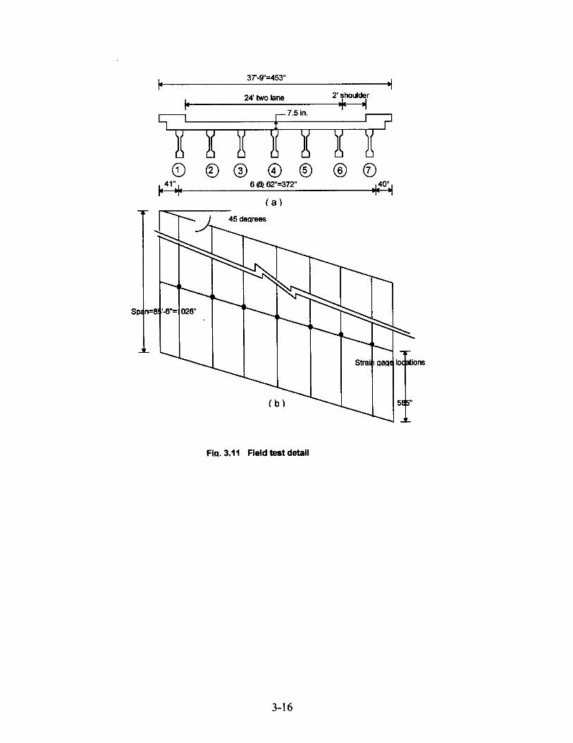
typical bridge to test the validity. The bridge is located on S.R. 17 and it consists of three simply supported

spans with the longest test span of 85'-6". The test span consists of 7 Type III prestressed concrete

girders, spaced at 5'-2" center to center and a slab thickness of 7.5 in. The skew angle is 45 degrees. The

bridge carries two lanes of traffic with curb to curb width of 26 ft. as shown in Figure 3.11. Table 3.1

summarizes the material and sectional properties of the bridge.

The measured strains along the bridge width at the maximum bending moment section are presented

in Table 3.2. The mesh and the finite element model for the bridge are similar to that of bridge #720408

which is presented in Chapter 4. Rigid links and simply supported boundary conditions were assumed in

modeling this bridge.

3-14

3-15

CHAPTER 4

LOAD DISTRIBUTION ANALYSIS OF SKEW

SLABON-GIRDER BRIDGES

4.1 INTRODUCTION

The slab-on-girder bridges are the most common type of bridges throughout the United

States. The precast concrete girders such as standard precast AASHTO 1-girders are efficient and

very economical. The precast concrete girders are often used with a cast-in-place deck to form the

riding surface. The major restrictions to precast girder construction are the limitations in the length

and weight. The slab-on-girder type bridges are practical for spans up to 120 ft. for AASHTO I-

girders.

Analyses performed during design of slab-on-girder bridges are commonly based on the

AASHTO wheel load distribution factors. There is a substantial amount of literature that

illustrates the conservatism in using the AASHTO wheel load distribution factors (Heins and

Lawrie,1984 and Warren and Malvar,1993). This led to the NCHRP to develop and propose the

LRFD simplified load distribution factors. However, advances in computing technology have

facilitated the use of refined analysis methods. In some cases, it is desirable to perform a more

advanced structural analysis. This is especially true, when an evaluation of the load capacity of an

existing bridge is being made. Finite element analysis can be used to obtain a more accurate and

reliable prediction of the load distribution factors.

4-1

The studies carried out by the Principal Investigator (Acrockiasamy,1995) on "Load

Distribution on Highway Bridges Based on Field Test Data - Phase I" present the load distribution

on certain non-skew bridge types in Florida viz., slab-on-girder, solid slab, voided slab and double-

tee bridges. Truck load distributions of skew slab-on-girder bridges based on finite element method

and field tests performed by Florida Department of Transportation (FDOT) are investigated in this

chapter. The objectives of this study are the following:

I) Determine the wheel load distribution using finite element method and study the effects of

skew angle, span length, girder spacing and slab thickness, exterior and interior girders and

other parameters.

II) Verify the AASHTO and the LRFD load distribution factors using several skew

slab-on girder bridge field tests.

III) Derive simple empirical design criteria, if needed, for load distribution that would provide more accurate alternative to current designs.

4.2 METHOD OF ANALYSIS

The measured field test data provided by Florida Department of Transportation was used in

conjunction with those based on the finite element models and AASHTO and LRFD bridge

specifications. Also, a parametric study for skew slab-on-girder bridges is conducted to identify the

main parameters. In the following sections, a summary of the AASHTO and LRFD specifications

is presented.

The AASHTO procedure to calculate the flexural distribution factors is generally used for

bridges and tends to be overly conservative particularly for analysis of existing bridges. The

4-50

AASHTO method of determining load distribution factors reduces the complex analysis of a bridge

subjected to one or more vehicles to the simple analysis of a beam. According to this method, the

maximum moment in a girder can be obtained by treating a girder as a one-dimensional beam

subjected to a loading, which is obtained by multiplying one line of wheels of the design vehicle by a

load fraction (S/D) where S is average beam spacing in ft. The quantity D in the AASHTO

specifications for concrete floor on prestressed concrete girders is 7 for one lane bridges and 5.5 for

mufti-lane bridges. If S exceeds 10 ft. for one lane bridges and 14 ft. for multi-lane bridges, the load in

each girder shall be the reaction of the wheel loads, assuming the flooring between the girders to act as

a simple beam. The AASHTO equation is based substantially on the research carried out by Newmark

(1948). The AASHTO equation did not include approximate formulae for moments to account for the

effects of skewed supports. It is frequently considered safe to ignore the skew angle, if it is less than 20

degrees and analyze the bridge with a span equal to the skew span, since it leads to a conservative

estimate of longitudinal moments and shears in the skew bridges. This approximate procedure is

inappropriate for old bridges and bridges with longer skew angles.

The LRFD approach is similar to AASHTO method, but considers more parameters such as

material properties, skew angle, sectional properties of the girders, span length, slab thickness, and

number of lanes. The LRFD approach is based on NCHRP project 12-26 entitled, "Distribution of

Wheel Loads on Highway Bridges", which was performed in two phases by Imbsen and Associates Inc.

The LRFD approach for slab-on-girder bridges gives different factors for bending and shear. The

distribution of live loads on precast concrete AASHTO I-girder is categorized under the category "K"

in the LRFD specifications. The LRFD distribution of live load moment in interior beams per lane is

given as:

One design lane loaded

4-51

4-4

cl = 0.25( K9 3 )0.25(5 )0.5

HOLts L If 0 < 30°, then cl = 0.0,

If 0 > 600, use 0 = 600,

The range of applicability of the Equation 5.4 is

30- <_ 0<_60', 3.6ft.<_S<16.Oft., 20ft.<_L<_240ft.

Both analytical and field studies on the truck wheel load distribution of skew slab-on-girders

are presented in this chapter. Finite element method explained in Chapter 3 is used to study the

various parameters affecting load distribution and suggest which parameters must be considered. In

addition to the analytical study, data from field tests performed by Structures Research center, MOT

are used to verify the analytical results.

4.2.1 Load Distribution Factor

A load distribution factor may be calculated from the strains of each girder determined from

finite element analyses or field tests. The distribution factor, DF is equal to the ratio of maximum

girder bending moment obtained from finite element method or field test to the total bending

moment in the bridge idealized as a one-dimensional beam subjected to one set of wheels.

The sum of internal bending moments is equivalent to externally applied bending moments

due to the wheel loads for a straight bridge. Assuming all traffic lanes are loaded with equal-weight

trucks, the wheel load distribution factor for the ith girder in a straight bridge is calculated from the

strains as follows ( Stalling and Yoo 1993):

DF ns; , _ (4.5) Y-J._ W. -1-*k sj J

4-5

E; = the bottom flange strain at the ith girder

W; = ratio of the section modulus of the ith girder to the section modulus of a typical interior girder

n = number of wheel lines of applied loading

Equation 4.5 is based on the assumption that the sum of the internal moments or the total

area under the moment distribution curve should be equal to the externally applied moment. This

assumption is valid only for straight bridges. However, this assumption is not realistic to yield the

actual moment distribution in skew bridges. The distribution factor, DF is equal to the ratio of

maximum girder moment obtained from finite element or field tests to the maximum moment in the

bridge idealized as a one-dimensional beam subjected to one set of wheels. The sum of the internal

moments in a straight bridge is equal to the maximum moment in the bridge idealized as a one-

dimensional beam subjected to one set of wheels. The sum of the girder strains in a straight bridge

will be used to take into account the total external load effects in skew bridges. Equation 4.5 can,

therefore, be modified as follows:

4-54

4.3 SKEW SLAB-ON-AASHTO GIRDER FLEXURAL LOAD

DISTRIBUTION FACTORS: PARAMETRIC STUDIES

It is important to understand the effect of various parameters on flexural load distribution.

Several parameters affect the load distribution of skew slab-on-girder bridges. Skew angle, span

length, girder spacing, thickness and load positions are the main parameters which are considered

in this section. Bridge parameters are varied one at a time in a typical bridge. Variation of wheel

load distribution factors with each parameter shows the relative importance of the parameters.

Figure 4.1 shows the typical skew slab-on-girder bridge used in the analyses. The typical skew

slab-on-girder bridge has a span length equal to 70 ft. with a bridge width of 54 ft and skew angle

of 30 degrees. It has prestressed AASHTO girder IV with a slab thickness of 7 in. The AASHTO

girder IV is shown in Figure 4.2. The concrete strength of both the girder and slab was taken

equal to 5,000 psi.

4.3.1 Finite Element Model

The typical skew slab-on-girder bridge is shown in Figure 4.1. The analysis assumes linear

elastic material behavior. The properties of the slab elements may have either isotropic or

orthotropic properties. Table 4.1 summarizes the material and sectional properties of the typical

bridge.

Typical top view of the finite element mesh is presented in Figure 4.3. The deck slab is

divided into 24 x 14 four-node shell elements and each girder divided into 24 sections. Simply

supported boundary conditions are realized by restraining the appropriate translational degrees

of freedom. Details of the modeling are presented in Chapter 3.

4-55

4.3.2 Truck Load Position

The AASHTO HS-20 truck was used in this parametric study (Figure 4.5). The truck load

position in the longitudinal direction (span direction) was located to produce the maximum bending

moment. To get the maximum bending moments in the bridges, two, three or four trucks were

positioned in the transverse direction.

Several cases were investigated to verify the critical load position. Figures 4.6 to 4.8 show

the different truck positions which were used to decide the critical load position for interior beam.

For exterior girders, the wheels of the first truck were at 3 ft. from the bridge edge, i.e. exactly over

the exterior girder as shown in Figures 4.9 and 4.10. Three cases were investigated to decide the

load position for exterior beam.

Table 4.2 summarizes the flexural load distribution factors calculated for different load

positions for both interior and exterior girders. Figures 4.8a and 4.9b show the selected critical

positions to calculate the load distribution factors for interior and exterior beam in this parametric

study for skew slab-on-girder bridge.

4-13

4.3.3 Parametric Studies

Table 4.3 summarizes the cases in which several parameters such as skew angle, span

length, girder spacing, slab thickness, etc., were considered to study the load distribution factors of

AASHTO girders. Thirty-two cases were investigated using finite element method (Ansys

Program) to establish the main parameters affecting the load distribution factors of the skew slab-

on-girder bridges.

4-20

4.3.3.1 Skew angle

Skew angle is ignored in the AASHTO code on load distribution computation, while the

LRFD code considers the skew effect by multiplying the non-skew distribution factors with a

reduction factor for both interior and exterior girders. The analysis based on finite element method

shows that skew angle is an important factor, which should be considered in the bridge design. Slab-

on-girder bridges with skew angles from 0 to 60 degrees (Table 4.3) were investigated in this section.

Four AASHTO HS-20 trucks were positioned in the transverse direction for interior girders,

while three HS-20 trucks were positioned for exterior girders. Figures 4.11 and 4.13 show the strain

distribution for a typical bridge with different skew angles. The strain decreases with the increase in

the skew angle and the strain distribution is more uniform for larger skew angles. These strain

distributions were used to calculate the distribution factors as explained in section 4.2.1.

Figures 4.12 and 4.14 show the changes in load distribution factors with increasing skew angles

for interior and exterior girders respectively. It is clear that DF decreases with increasing skew angle

for interior and exterior girders. For interior girders, the distribution factors calculated from the

finite element method are smaller than those from the LRFD code. And the difference decreases with

a corresponding increase in the skew angle. For exterior girder, the distribution factors from F.E.M.

are also smaller than those from the LRFD code. The skew angle has similar effects on the load

distribution factor, DF for both interior and exterior girders.

4-21

4.3.3.2 Span length

Span length is one of the main factors in load distribution of slab-on-girder bridges. The

AASHTO code ignores span length effect on load distribution, while the LRFD code considers the

span length as an important factor in wheel load distribution. The span length was varied between

50 ft. to 100 ft. as shown in Table 4.3.

Figures 4.15 and 4.17 show the strain distributions for typical skew bridges with different span

lengths for interior and exterior girders respectively. The strains increase with the increases in the

span length and strain distribution tends to be more uniform for shorter spans. The strain

distributions were used to calculate the distribution factors. The D.F. calculations were based on

Equation 4.5 instead of equation 4.6. The DF difference was negligible (1.5 - 5 %).

Figures 4.16 and 4.18 show the changes in load distribution factors with increasing span

length for interior and exterior girders respectively. The load distribution factors of the interior

girders decrease with increasing span and the load distribution factors of exterior girders increase

with span increase.

AASHTO codes gives the same load distribution factors for different spans of a typical bridge. The

load distribution factors calculated from the finite element method are smaller than

4-22

4-23

those from AASHTO code for interior girders. The difference only slightly increases with the

corresponding increase in span length. It shows the AASHTO code gives a safe estimate of

distribution factors. For exterior girders, the distribution factors based on finite element method

are larger than those calculated from AASHTO code. This means that the AASHTO code gives

unsafe estimate of distribution factor, DF for exterior girder.

The load distribution factors based on LRFD code show a significant decrease with the

increase in span length for both interior and exterior girders. Figures 4.16 end 4.18 show that the

LRFD load distribution factors are less accurate for shorter spans.

4.3.3.3 Girder spacing

Girder spacing is an important factor in load distribution of slab-on-girder bridges and it is

the only parameter considered in the AASHTO code. The spacing between AASHTO girders was

varied from 6 to 12 ft. as shown in Table 4.3.

Figures 4.19 and 4.21 show that the strain distribution for typical bridge with different girder

spacings for interior and exterior girders respectively. The strains increase with the increase in

girder spacing for both interior and exterior girders. The strain distribution is more uniform for

smaller girder spacing. The load distributions were used to analyze the effect of girder spacing on

load distribution factor. The D.F. calculations were based on Equation 4.5 instead of equation 4.6.

Figures 4.20 and 4.22 show that the load distribution factors, DF increase with the increasing girder

spacing for interior and exterior girder respectively. The DF for interior girders is more dependent

on girder spacing, S than the exterior girders. In general, the girder spacing is a very important

factor in determining wheel load distribution.

4-25

The load distribution factors calculated from finite element method are smaller than those based on AASHTO code for interior girders and the difference in the values is almost the same

with the increase in girder spacing. So AASHTO code gives a conservative and reliable estimate of

load distribution factor for interior girders. For exterior girders, the DF from finite element method

are larger than those based on AASHTO code.

The LRFD distribution factors are smaller than those calculated from finite element method

for interior girders particularly for larger spacing while they are larger for exterior girders. The

wheel load distribution based on AASHTO, LRFD code and Finite Element Method are generally in

good agreement when the girder spacing effect is considered.

4-77

4.3.3.4 Slab thickness

AASHTO code ignores the slab thickness as a parameter in wheel load distribution, while

LRFD code considers the thickness effect on load distribution. Skew slab-on-girder bridges with

slab thickness varying approximately from 4 to 7 in. are investigated in this section.

The strain distributions for different thicknesses are shown in Figures 4.23 and 4.25 for interior and

exterior girders respectively. The maximum strain decreases with the increase in thickness and the

strain distribution tends to be more uniform.

Figures 4.24 and 4.26 show the change in load distribution factors with the increasing slab

thickness. The AASHTO load distribution factors are the same for different slab thicknesses, and for

both interior and exterior girders. For interior girders, the DF calculated from finite element method

are smaller than those based on AASHTO code and slightly decreases with the increasing slab

thickness. For exterior girders, the DF from F.E.M. are larger than those from AASHTO code when

the slab thickness becomes large. In general, AASHTO code can give a safe estimate of DF when

the slab thickness is considered.

For both interior and exterior girders, the load distribution factors based on LRFD code

show a significant reduction with the increase of slab thickness. The LRFD code load distribution

factors are larger. than those calculated from finite element method. Both AASHTO and LRFD can

4-78

4.4 SKEW SLAB-ON-AASHTO GIRDER BRIDGES: FIELD

TESTS Florida Department of Transportation (FDOT) have tested many bridges to check the

strength. The strength of bridge elements is generally determined by first installing the strain or

deflection transducer gages at the bridge critical locations along the girders, and then

incrementally loading the bridge to induce maximum effects. The data collected can then be

analyzed and used to establish the strength of each component as well as the load distribution.

The FDOT's bridge load testing equipment consists of two test vehicles, a mobile data

acquisition system and a mobile machine shop. The two test vehicles have been designed to

deliver the ultimate live loads specified by AASHTO code. Each vehicle can carry a maximum of

72 concrete blocks, each weighing approximately 2,150 pounds. Incremental loading is achieved

by adding blocks with a self-contained hydraulic crane on each truck.

The test vehicles are initially loaded with a number of concrete blocks, established from the

preliminary analysis of the existing structure. The vehicles are then driven and placed on the critical

locations of the bridge. After each load step, the measured strain and deflections are compared with

the theoretical predicted values and additional blocks are then added to the vehicles and the test

repeated until the ultimate AASHTO load is achieved. The data gathered can then be analyzed and a

report of the findings prepared.

Data from certain slab-on-AASHTO girder bridge test reports are used in the load

distribution analyses. The typical report contains transverse strain distributions in the maximum

bending moment section for several load stages. The report also contains the applied moment vs.

strain curves for several load stages.

4-83

The girder bending moment can be calculated from the measured strains as follows:

M = E E S (4.7)

where

E = the strain measured at the extreme fibers of the bottom

flange E = the modules of elasticity

S = the section modulus

The ACI equation was used to calculate the elastic modulus of concrete which is based on f,' =

5000 psi. Many bridges exhibit some degree of composite action even when they were not constructed

with shear studs or other devices for transferring shear between girders and deck. The composite and

non-composite section modulus were used to calculate the measured bending moments. The use of

composite section modulus overestimates the measured bending moments. The use of cracked section

modulus may be more realistic in the calculation of the bending moment based on the measured

strains.

The skew angle for all the tests were less than 30 except for field test # 2, therefore

Equation 4.5 were used instead of Equation 4.6 in the load distribution calculations for all the tests.

For tests where all traffic lanes are loaded with equal-weight trucks, the measured wheel load

distribution factor for the ith girder is given as [Stallings and Yoo(1993)]

DF, - ns; (4.5)

Where

8; = the bottom flange strain at the ith girder,

4-84

k = number of girders,

n = the number of wheel lines of applied loading

The parameter, n is required to make the measured wheel load distribution factor compatible with

AASHTO definition. In this chapter, similar approach was used to calculate the measured load

distribution factor based on the calculated bending moments. The measured distribution factor is

compared with those based on AASHTO, LRFD and finite element analyses.

4.4.1 Duval County Bridge (#720408)

The bridge is located on I-295 over S.C.L.R.R. and U.S 90, in Duval county

(Jacksonville, Florida). It consists of 7 simply supported spans with span lengths of 56', 104.15',

62.13', 64.23', 79.56' and 60.50 feet respectively. The length of tested span is 104.15 ft with a

skew angle of 17.48 degrees. The span consists of 8 Type IV prestressed concrete girders, spaced

at 5.30' center to center and slab thickness of 7.0 in. The bridge carries two lanes of traffic with

curb to curb width of 40.0 ft. as shown in Figure 4.27. Table 4.4 summarizes the material and

4-85

Instruments for measuring strains were placed at critical locations on the tested span. The bridge was

loaded with two trucks incrementally with 36, 48, 60 and 72 blocks respectively. The strain readings

were taken at each load increment to establish the behavior of the bridge. The load case

corresponding to sixty blocks has been used in the analysis to ensure the strains are within the linear

and elastic range.

Typical top view of the Finite Element Mesh is presented in Figure 4.28. Each node had six degrees of

freedom and the nodes were arranged such that some nodes were located at the strain gage positions

to facilitate the comparison between the measured and calculated strains The deck slab is divided

into 16 x16 = 256 four node-shell elements and each girder divided into 16 sections. The I-girder

section is discretized into three elements as shown in Figure 4.4. Each flange is modeled by a beam

element with four midsurface nodes. The rigid links ensure coupling the vertical degrees of freedoms

of the shell and top flange beam elements. Simply supported boundary conditions are realized by

restraining the appropriate translafional degrees of freedom.

Table 4.5 summarizes the results from the finite element analysis and field test at a cross section corresponding to the maximum bending moment location. Figure 4.29 shows the comparison of the measured and calculated strain distribution along the bridge width. It is clear that the measured and calculated strains show good agreement. However, a better correlation may be achieved, if the actual boundary conditions and more accurate truck positions were available.

Table 4.5 Measured and calculated strains for bridge #720408

Table 4.6 summarizes the results of wheel load distribution factors for the bridges based on the measured strains, finite element method, AASHTO and LRFD codes. The measured wheel load distribution factor, DF compares well with calculated DF. Both DFs based on AASHTO and LRFD were higher than the DF calculated using the measured strains and finite element method. This confirms that AASHTO and the LRFD code give conservative values for wheel load distribution factor for skew slab-on-girder bridges.

4-91

4.4.2 S.R.17 Bridge #720089

The bridge is located on S.R. 17 and it consists of three simply supported spans with the

longest test span of 85'-6". The length of the total structure is 181'-6". The span consists of 7 Type

III prestressed concrete girders, spaced at 5'-2" center to center and a slab thickness of 7.5 in. The

skew angle is 45 degrees. The bridge carries two lanes of traffic with curb to curb width of 26 ft. as

shown in Figure 4.30. Table 4.7 summarizes the material and sectional properties of the bridge.

The arrangement of instruments and the location of the strain gages is similar to that of

bridge #720408 (Section 4.4.1). The measured strains along the bridge width at the maximum

bending moment section are presented in Table 4.8. The mesh and the finite element model for the

bridge are similar to that of bridge #720408 which is shown in Fig. 4.28, while the deck slab is

divided into 16 x 14 = 224 eight node-shell elements. The rigid links and simply supported

boundary conditions are also applied to this bridge.

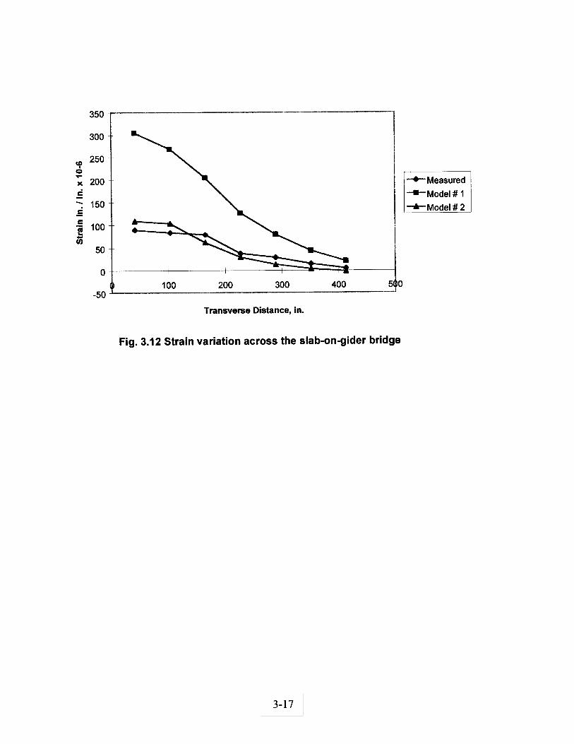
Table 4.8 summarizes the results from finite element analysis and field test at a cross

section corresponding. to the maximum bending moment location. Figure 4.31 shows that the

measured and calculated strain distribution along the transverse direction. In this bridge, the finite

4-92

element method strains were consistent with those based on measured strains. The DF from

measured strains is smaller than the calculated strains from finite element method. Both DFs

from calculated and measured strains are smaller than those based on AASHTO and LRFD codes

as shown in Table 4.6. This again confirms that both AASHTO and LRFD codes give conservative

estimate for wheel load distribution factors.

4.4.3 Turnpike Bridge over 1-595 The bridge is located on the Florida Turnpike over Interstate 595. The bridge was completed in the summer of 1989. This twin structure consists of identical northbound and southbound bridges with 5 spans of simply supported AASHTO girders 130 ft., 151 ft., 99 ft., 99 ft. and 99 ft. in length respectively. Span 2 which was chosen as the test span consists of twelve simply supported AASHTO Type V girders and the girders are spaced at 5'-11" center to center. The bridge is 68' wide from curb to curb and carries four 12 ft. lanes and two 10 ft. shoulders with typical crash barriers on either side. The slab is 7 in. thick and the bridge is skewed 20 degrees. The bridge was constructed using an innovative shoring system which allows the section to act compositely for dead load as well as for live load. The details of the bridge are shown in Fig.4.32. Table 4.9 summarizes the material and the sectional properties of the bridge.

The instrumentations are mounted at critical locations of the structure and connected to the data acquisition system. The bridge was loaded with two trucks and the load case corresponding to the trucks weight of 24 kips each has been used in this analysis. The measured deflection along the bridge at the maximum bending moment are presented in Table 4.10. The mesh and the finite element model for this bridge are similar to that of the bridge #720408 shown in Figures 4.28 and

4-47

4.29 except the deck slab is divided into 30 x 24 = 720 four node shell-elements, and each girder

divided into 30 sections. The rigid links and the simply supported boundary conditions are applied

to the bridge.

The results from the finite element method and field test at midspan section along the bridge width

is shown in Table 4.10. Figure 4.33 shows the comparison of the measured and calculated strain

distributions along the bridge width. It can be seen from the figure that the measured deflections

are smaller than the analytical values. But it can also be seen that the finite element method

predicts the behavior and load distribution of the bridge fairly well. The results show that the

overall behavior of the bridge is quite adequate.

The measured wheel load distribution factor, DF was smaller than that from the finite element

method as shown in Table 4.6. But both DF from finite element method and field test are smaller

than those based on AASHTO and LRFD values. This shows that AASHTO and LRFD code give

conservative estimate of wheel load distribution factor for skew slab-on-girder bridge.

CHAPTER 5

LOAD DISTRIBUTION ANALYSES OF SKEW

SOLID SLAB BRIDGES

5.1 INTRODUCTION

Solid or voided sections are used in slab bridges, which span between supports in the

longitudinal direction, i.e., traffic direction. Concrete slab bridges are economical for spans in the

range of 10-26 ft. However, spans up to 50 ft. can also be feasible. These bridges are normally

reinforced with reinforcing bars, but prestressing strands and I-beams have also been used in

practice. They also offer a smaller structure depth where structure opening and vertical clearance

are significant. In addition to the above advantages, slab bridges are commonly used due to its low

construction cost.

Skew bridges have been designed for many years using approximate methods. Most of these

methods do not account for high torsional moments inherent in a skewed structure. More exact

methods of analysis are time consuming. In this chapter, an exact method such as finite element

method is used to verify/modify the AASHTO-LRFD load distribution factor of skew slab bridges.

Wheel load distribution on solid slab bridges based on both finite element method and field tests

performed by Florida Department of Transportation (FDOT) is presented in this chapter. The

objectives of the analyses are the following:

i) Determine the effective width using finite element method and study the effects of skew

angle, span length, edge beam depth and other parameters on wheel load distribution.

5-1

ii) Verify the AASHTO and the LRFD effective widths using simply supported skew slab

bridge field tests.

iii) Derive simple design criteria for effective width that would provide more accurate

alternative to current designs.

5.2 METHOD OF ANALYSIS

The Finite Element Method is used to verify the effective widths based on the AASHTO

and LRFD wheel load distribution methods. The AASHTO procedure to determine the flexural

distribution factors is generally used for bridge design and tends to be overly conservative

particularly for analyzing and rating of existing bridges, which may cause unnecessary rerouting

of vehicles in certain circumstances (Warren and Malvar,1993). The AASHTO approach is to

calculate an effective width E, over which the concentrated wheel load (half truck load) is

assumed to be uniformly distributed (AASHTO specification, 1989)

E = 4.0 + 0.06S (feet) ( E < 7 ft.) (5.1)

Where S = span length, in feet. A larger value of E means more efficient distribution of the load.

Slab thickness and flexural reinforcement are then determined from an equivalent strip of width

2E carrying the total truck load. The AASHTO equation is based substantially on Westergaard

theory for slabs (Westergaard, 1930). The AASHTO equation considers span length as the only

parameter and neglect other important parameters such as skew angle, edge beam, etc.

5-101

The LRFD approach is similar to AASHTO method, but considers more parameters such as skew

angle, bridge width and number of lanes. The LRFD approach is based on NCHRP project 12-26

entitled, "Distribution of Wheel Load on Highway Bridges", which was performed in two phases

by Imbsen & Associates, inc.(1989). The LRFD approach for slab bridges was based on limited

number of analytical studies. The LRFD effective width of longitudinal strip per lane for both shear

and moment with one lane, i.e., two lines of wheels, loaded may be determined as follows:

where,

9 = Skew angle (DEG)

Finite element method (ANSYS Program) presented in Chapter 3 is used as an analytical

tool to study the various parameters affecting load distribution and suggest which parameters should

be considered. In addition to the analytical study, data from field test performed by Structures

Research Center, FDOT, are used to verify the results from the analytical study.

5.2.1 Effective Width Calculation

An effective width may be calculated from the distribution of moments determined from the

finite element method and field tests. The sum of moments or the total area under the moment

distribution curve is equivalent to externally applied moment due to the concentrated loads

(including the edge beam moments). The effective width, E is equal to the ratio of the total area

under the moment distribution curve to the maximum moment. This method of calculating E is

based on the assumption that the sum of the internal moments or the total area under the moment

distribution curve should be equal to the externally applied moment. This assumption is valid only

for straight bridges. However, this assumption is not realistic to yield the actual effective width in

skew bridges. The effective width, E is equal to the ratio of the maximum moment in the bridge

idealized as a one-dimensional beam subjected to one set of wheels to the maximum moment

intensity obtained from finite element or field tests. The sum of the internal moments in a straight

bridge is equal to the maximum moment in the bridge idealized as a one-dimensional beam

subjected to one set of wheels. The sum of the internal moments in a straight bridge will be used to

take into account the total external load effects in skew bridges. Therefore, E can be obtained for a

5-103

(Y- moments__

Ee (5.5) (Moment m..) B

5.3 SKEW SOLID SLAB BRIDGE: PARAMETRIC STUDY

Several parameters affect the load distribution of skew solid slab bridge. Skew angle, span

length, and edge beam depth are the main parameters which are considered in this section. Figure

5.1 shows the typical slab bridge cross section which is used in the analysis. The typical slab bridge

has a span length of 21 ft. with a width equal to 30 ft. and the slab thickness of 12 inch..

5.3.1 Skew Slab Bridge Finite Element Modeling

The typical skew slab bridge cross section is shown in Figure 5.1. Linear elastic material is

considered in the modeling. The slab elements are considered to be isotropic. Table 5.1 summarizes

the material (Elastic modulus, E, Poisson's ratio, v, and modulus of rigidity, G) and sectional

properties of the bridge (Area, A, and moments of inertia, ly and I.J.

Typical top view of the skew solid slab bridge finite element mesh is presented in Figure 5.2.

Generalized shell elements coupling bending with membrane action were used to model the skew

slab bridge. The shell elements were proportioned so that the maximum aspect ratio always remains

at two to one or less (Chen,Y. 1995). Each node has six degrees of freedom and the nodes are

arranged such that some nodes were located at the critical positions. The skew slab bridge is divided

into 12 x 22 = 264 four-node shell elements. Simply supported boundary conditions are obtained by

restraining the appropriate translational degrees of freedom along the edges.

Two models shown in Figure 5.3 were used in the parametric study. Only shell elements are

used to model slab and the edge beams were neglected in Model 1. Beam elements are added to

5-5

model the edge beams in Model 2. The skew slab was modeled using shell element with 4 or 8

nodes. The difference in accuracy of results based on the two types of elements was small and the 4

node shell elements were used throughout the parametric study.

5-6

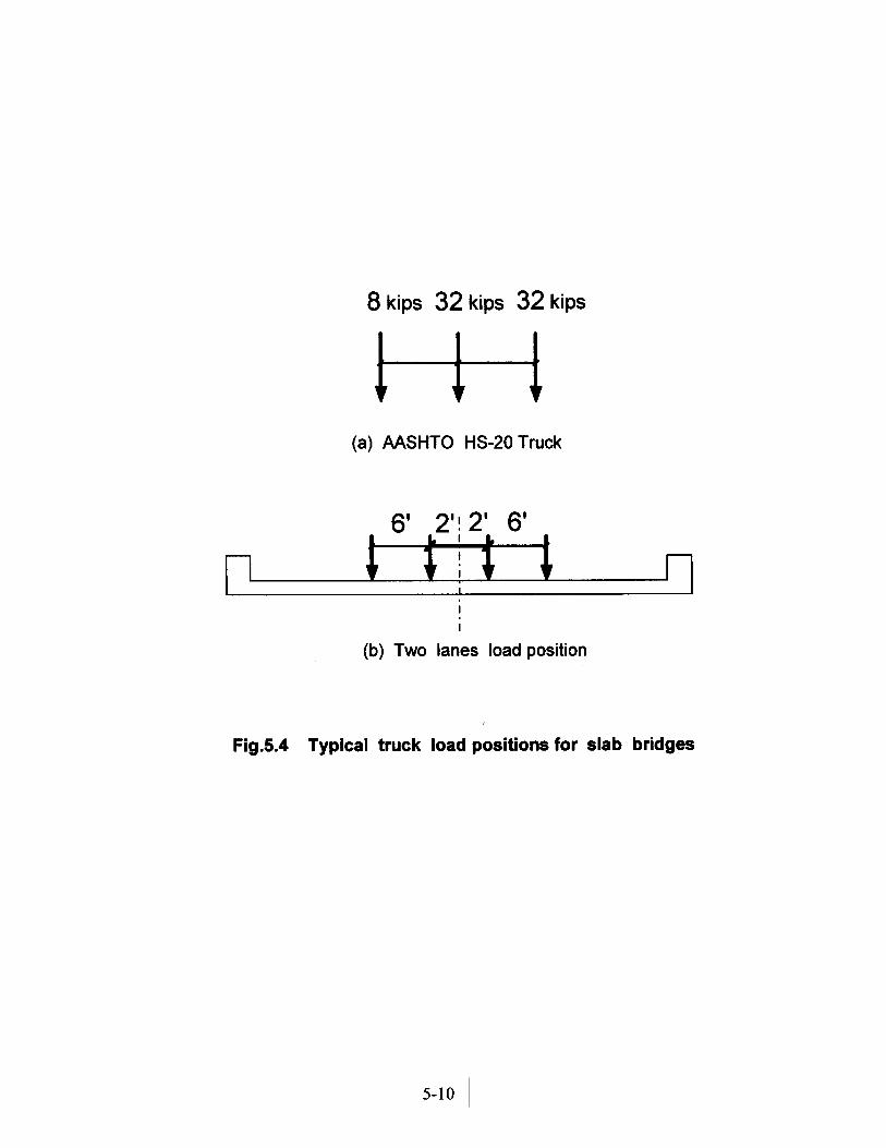
5.3.2 Truck Load Position

The AASHTO HS-20 truck was used in this parametric study. The truck position in the

longitudinal direction (span direction) was located so as to obtain the maximum bending moments.

For skew slab bridges with relatively short spans, the maximum bending moment occurs when

only one axle of the truck is at the midspan. For a two lane slab birdge, it was found that the

maximum bending moment occurs when the two lanes are loaded as in Figure 5.4b. Since the

locations of wheel loads will probably not coincide with nodes of the shell elements, it is necessary

to calculate the equivalent nodal loads. To this end, the concept of tributary area can be used to

determine the equivalent loads as explained in Chapter 3.

The exact load positions for the typical skew solid bridge are shown in Figures 5.5 and 5.6. Two

different load positions were used to find out the effect of load position. The span length of the typical

bridge is 21 ft which is a relatively short span, so the maximum moment will be at the midspan. But

the axles of the trucks must be perpendicular to the traffic direction, hence two wheels of a truck

cannot be at the midspan at the same time due to the skew angle. All the maximum moments are taken

at the mid span. The comparison of the moment distribution for two different load positions is shown

in Figure 5.7. The moment distribution is not a smooth curve because some of the wheels are away

from the midspan. The moment distribution due to load position 2 shifts away from that due to load

position l. But the trends are the same. Load position 1 is used throughout the parametric study for

skew solid slab bridges.

5-9

5.3.2 Parametric Studies

Table 5.2 summarizes the cases and the several parameters such as skew angle, span length and

edge beam depth considered in the study. Twenty-four cases were investigated using linear finite

element method to establish the main parameters affecting the effective width of the skew solid slab.

5.3.2.1 Comparison of two models

Table 5.3 summarizes the results from the two models at the critical cross section for typical

slab bridge. The effective widths calculated from the two models are presented in Table 5.4. The

moments at the positions where edge beams were located reduce with the addition of beam elements

and the maximum moment also reduces. Figure 5.8 shows the comparison of moment distributions

along the width, which shows that the curve is steeper than that of model l. The effective width

calculated from model 2 is smaller than that from model 1 and it seems more conservative and less

significant.

5-14

5.3.2.2 Skew angle

Skew angle is one of the main factors affecting load distribution in slab bridge. Solid slab

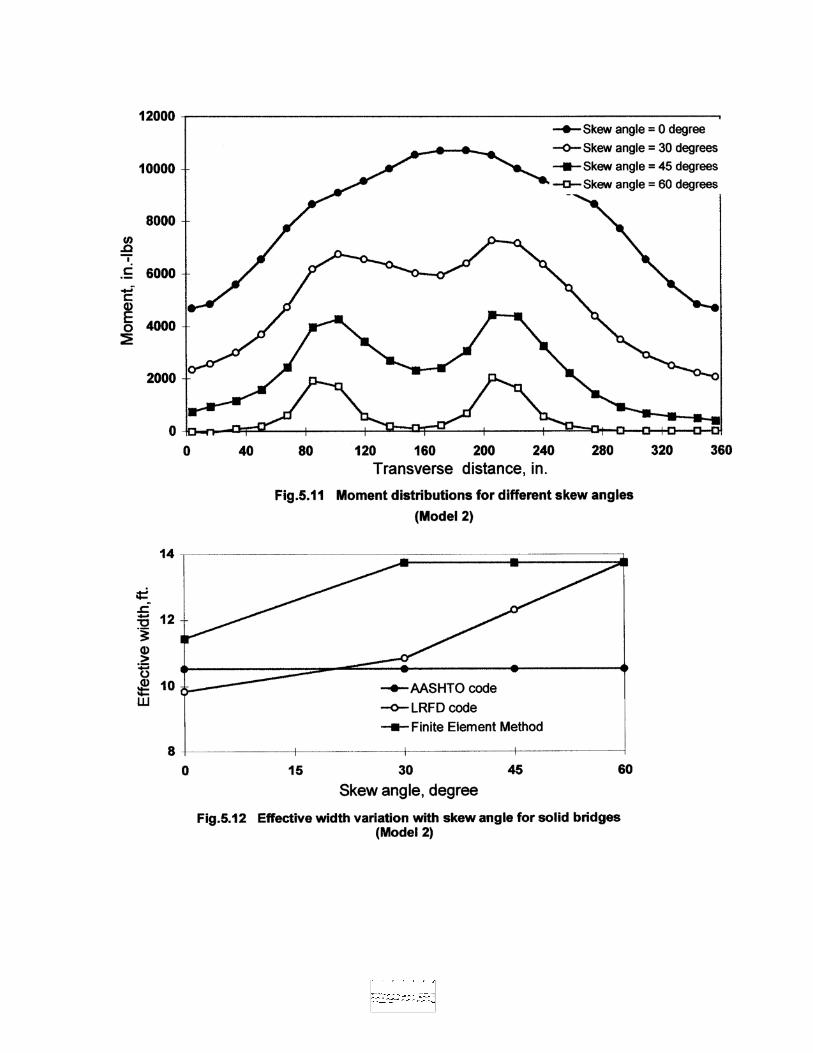
bridges with skew angles from 0 to 60 degrees (Table 5.2) were investigated in this study. Figures

5.9 and 5.11 show the strain distributions for typical bridges with different skew angles. The

moment decreases with the increase in the skew angle and the moment distribution is more

uniform for smaller skew angle. Larger effective widths are obtained with increase in the skew

angle. These moment distributions were used to calculate the solid slab effective widths.

Figures 5.10 and 5.12 show the effective widths increase with the increasing skew angle for

both models. In the cases where the effective width based on the finite element method exceeded

the lane width, the effective width was assumed equal to the lane width of 13.75 ft. The effective

widths calculated from finite element analyses are generally larger than those calculated using

AASHTO and LRFD codes as shown in Figures 5.10 and 5.12. This means that AASHTO and

LRFD codes give a more conservative estimate of effective width, E for solid slab bridges. It

seems reasonable that the skew angle should be considered in the calculation of effective width.

Model 2 which uses slab and edge beam elements gives smaller moments than model 1

which only uses slab elements in modeling the bridge. Figure 5.13 shows the effective width

calculated based on model 2 is smaller than that based on model 1 The difference in the estimated

effective width value vanishes with the corresponding increase in the skew angle because all the

values are higher than the lane width and taken equal to the lane width.

5-18

5.3.2.3 Span length

Span length is an important parameter which is considered in both AASHTO and LRFD

codes. The span length for the typical bridge was varied between 15 ft. to 40 ft. as shown in Table

5.2. Figures 5.14 and 5.16 show the moment distributions for typical bridge with different span

lengths. The moment increases with the increase in the span length for both models. And a larger

effective width is obtained corresponding to a larger span length.

Figures 5.15 and 5.17 show that the effective width increases with increasing span length. The

change in effective width is significant and hence span length cannot be neglected in the bridge

design. The effective widths calculated based on the finite element method are larger than those

based on AASHTO and LRFD codes. This indicates that both LRFD and AASHTO code give

conservative estimates of effective width, E when span length is considered. Model 2 is a better

model since it gives smaller moments and effective width than those of model 1.

5-22

5.3.2.4 Edge beam depth

AASHTO code requires that an edge beam should be provided for longitudinally

reinforced slabs (main reinforcement parallel to traffic). The edge beam of a slab bridge with

simple span should be designed for a live load moment of 0.1OPS, where P = wheel load in

pounds and S = span length in feet (AASHTO, 1989). One interpretation of this requirement could

be that approximately 40% of the live load moment caused by one line of wheels (maximum

moment for one line of wheel load in short span is approximately 0.25 PS) should be added to the

other computed moment for the width selected for the edge beam. The width of edge beam as

required by AASHTO specifications, should not exceed 3 feet.

The LRFD code requires that the edge beams shall be assumed to support one lane of

wheels, and where appropriate, a tributary portion of the design lane load (LRFD section

4.6.2.1.4a).

Although edge beam is a very important parameter in load distribution, it is neglected in both

AASHTO and LRFD effective width calculations. Figure 5.19 shows the moment distribution for

different edge beam depths. Model 1 does not consider the edge beam element, therefore, Model 2

moments and effective widths are presented in Figs. 5.19 and 5.20. With the increase of edge

beam depth, the maximum moment slightly decreases as shown in Figure 5.19. Consequently, the

calculation shows that effective width, E decreases with the increase of edge beam depth. All the

E values were larger than the lane width, therefore, E was assumed equal to the lane width of

13.75 ft as shown in Figure 5.20.

Figures 5.20 and 5.21 show the change in effective width with increase in the edge beam

depth. The effective widths calculated using finite element method are larger than those calculated

5-125

using AASHTO and LRFD codes. This means AASHTO and LRFD codes give conservative

estimate of effective width when the edge beam depth is considered. And these results suggest

that the edge beam size should be taken into account in wheel load distribution. Neither

AASHTO code nor the LRFD code considers the edge beam moment of inertia in the effective

width equation.

5.3.3 Proposed Simplified Effective Width for Solid Slab Bridges

Based on the straight solid slab bridge parametric studies (Study Phase 1, Arockiasamy

and Amer, 1995), the span length and the edge beam depth are the main parameters, which

significantly affect the effective width calculations. For straight solid slab bridges without edge

beams or with hidden edge beams, the following equation based on the least square fit of the

grillage analogy results (Phase I of this study) for the effective width could be used for spans

upto 40 ft. and slab thickness upto 14 in.:

E = 6.89 + 0.23 L <_ W/NL (5.8)

where

E = Effective width over which truck load is assumed to be uniformly distributed,

ft. L = Span length, ft.

W = Physical edge-to-edge width of bridge ,(feet.units),

NL = Number of design lanes.

The effect of edge beam depth above the slab thickness can be taken into consideration

by multiplying the above equation by a factor Ce* given by

5-126

where d, = Edge beam depth above the slab thickness, in.

Based on the finite element results in this study (Phase 11), it can be concluded that the

effective width increases with the skew angle increases for solid slab bridges. This confirms the

LRFD codes in considering the skew angle as a parameter in effective width calculation. The finite

element results show the same skew angle effects as those in LRFD codes except for higher skew

angle than 45 degrees where the effects are higher in finite element than in the LRFD code.

Therefore, the LRFD moment reduction factor due to skewness of solid slab bridges will be used to

modify the proposed simplified effective width for straight solid slab bridges.

For skewed bridges, the effective width can be enlarged by:

Cse„,= (1/r)=1/(1.05-0.25tan0) where( r<_ 1.00)

where,

5-28

5.4 SKEW SOLID SLAB BRIDGE FIELD TEST

Florida Department of Transportation (FDOT) have tested many solid slab bridges to check

their strength. The bridges are first instrumented for measuring strains and deflections at the bridge

deck critical locations, and then incrementally loaded to induce maximum effects. The data

collected are then analyzed and used to establish the strength of each component as well as the load

distribution.

The test vehicles are initially loaded with a number of blocks of known weights, established from the preliminary analysis of the bridge. The vehicles are then driven and placed on the critical locations of the bridge, while the strains and deflections are monitored using the data acquisition system during loading. After each load step, the measured strains are compared favorably with the theoretical predictions, additional blocks are added to the vehicles and the test repeated until the ultimate AASHTO load is achieved. The data are then processed to determine the load distribution.

Test data from typical solid bridges are used for load distribution analyses. The typical test

report contains transverse strain distribution in the maximum bending moment section for several

loading stages. It also contains the applied moment vs. strain curves for several loading stages.

The bridge load test data are used in the determination of wheel load distribution factors, i.e.

effective width, E. The measured effective width can be used in bridge-rating calculations in place

of effective width defined by AASHTO.

In the present study, the measured strains will be multiplied by the slab section modulus and

the elastic modulus to calculate the measured moments. The ACI equation was used to calculate

the elastic modulus of concrete which is determined based on flc = 5000psi. The measured strain

distribution is used to calculate the effective width, which is compared with those based on

AASHTO, LRFD and finite element method.

5.4.1 Collier County Bridge (#030144)

The bridge is built in 1963 and located on Tamiami Trail HWY41 in Collier County (Bartow,

Florida). It consists of five simply supported spans with span lengths of 21 feet each. The total length

and width of the bridge are 105 feet and 46'-3" respectively with curb to curb width of 44'-0". The

bridge is two lane skew bridge with skew angle of 14.28 degrees as shown in Fig.5.25. The bridge is a

concrete flat slab type, with 12.5 in. thick deck supported by concrete bent cap and concrete piles. An

inspection of the bridge showed that the slabs, piles and pile caps along the entire length of the

bridge to be good condition, except for the transverse slab cracks over each support (bent cap).

Table 5.5 summarizes the material properties of the bridge.

Instrumentation for measuring the strains were placed at the critical locations on the test span

(northwest span). The bridge was incrementally loaded with two trucks (24, 30, 36 and 42 blocks).

The strain and deflection readings were taken at each load increment to establish the behavior of the

bridge. The load case corresponding to thirty blocks have been used in the analysis to ensure the

behavior of the bridge was within the linear and elastic range. The measured strains along the bridge

width at the maximum bending moment section are presented in Table 5.6.

5-32

Typical top view of the finite element mesh is presented in Figure 5.23. Each node had six

degrees of freedom and the nodes arranged such that some nodes were located at the strain gage

position to facilitate the comparison between the measured and calculated strains. The slab is

divided into 24 x14 = 336 four-node shell elements. Simply supported boundary conditions are

realized by restraining the appropriate translational degrees of freedom.

Table 5.6 summarizes the results from finite element analysis and field test at a cross section

corresponding to the maximum bending moment location. In general, the maximum slab deflection

of 0.138 in. obtained from analysis agree well with the measured value of 0.14 in.. Figure 5.24 shows

the comparison of the measured and predicted strain distribution along the bridge width. It is clear

that the measured and calculated strains at the bottom of the slab show a significant difference. The

difference in measured strain values could be attributed to observed transverse cracks on the

bottom of the slab. These cracks open under the applied loads and consequently produce higher

strains in the bottom of the slab. However, the local cracking is not modeled in the finite element

analysis. This observation indicates that limited local cracking of the slab does not affect the global

measured response of the bridge to applied loads and computed displacements are in good

agreement.

5-33

Table 5.7 shows the effective widths calculated by different methods. The values calculated from finite element method and field test are higher than those from AASHTO and LRFD codes. The effective widths based on the AASHTO and LRFD codes are conservative.

5-37

CHAPTER 6

LOAD DISTRIBUTION ANALYSIS OF

CONTINUOUS SLAB-ON-GIRDER

BRIDGES 6.1 INTRODUCTION The design of highway bridges has followed the guidelines of the American Association

of State Highways and Transportation Officials (AASHTO) or Load and Resistance Factor

Design (LRFD). The AASHTO and LRFD codes do not specify any modification for computing

the distribution factors for continuous bridges as they do for single span skew bridges. LRFD

bridge design specifications (1994) deleted the wheel load distribution correction factors for

continuity from the LRFD specifications. The code commentary gives the following reasons for

deleting the correction factors: the value of the correction factors were within 5%, which is less

than the level of the accuracy for the approximate distribution factor method, and the increase in

the distribution coefficient for negative moments tends to cancel out when the distribution of

reaction force over the bearing is considered. Other publications have recognized the need for

more research to examine the importance of the correction factor for continuity (Khaleel, Itani

1990). Alternative designs for continuous bridges have taken a direction in which computer

models using finite element method (FEM) accurately predict the bridge behavior for various

loadings.

Research on continuous bridges has mostly been limited to the analysis of two-

dimensional models to obtain the moments, shears, rotations, and deflections. AASHTO design

6-1

considers a single girder that acts compositely with a concrete deck. This composite section carries a portion of a designated wheel load that is distributed transversely to the girder (AASHTO 1992). Continuous bridges amplify the complexity of solving a two or three dimensional problem. FEM does accurately predict solutions for specific bridges. A 0.4-scale model of a two-span bridge comprised of concrete deck on steel girders, was loaded with simulated truck loads. The results of the study show that FEM predicts the reactions, moments, displacements, and rotations with a high accuracy of + 10% (Tiedman, Albrecht, Cayes 1993). The accuracy of the FEM analysis of continuous bridges is dependent on the type of the model. Each model has different elements, material properties, and boundary conditions which should be considered individually and evaluated to serve as a basis for establishing accurate predictions for continuous bridges.

The objectives of this study on continuous bridges are:

i) Study the effects of bridge skew angles, number of spans, span ratio between two

spans, and other parameters on load distribution factors using FEM.

ii) Compare AASHTO, LRFD, and FEM load distribution factors with those based on

field tests on continuous bridges.

iii) Recommend new methods/changes, if needed, for calculating wheel load distribution

factors for continuous bridges based on correlation of field tests and FEM analysis.

6.2 METHOD OF ANALYSIS

The continuous bridge analyses using AASHTO and LRFD codes, FEM, and field test

data were used to establish load distribution guidelines . The AASHTO approach is based

substantially on Westergaard theory for slabs (Westergaard, 1930). The LRFD method is based on

NCHRP nroiect 12-26 entitled, "Distribution of Wheel Load on Highway Bridges", which was

6-2

performed in two phases by Imbsen & Associates, inc.(1989). FEM distribution factors are

calculated based on moment distribution ( Stalling and Yoo 1993). The following section

summarizes the method of analysis.

6.2.1 AASHTO and LRFD Distribution Factor

There are no AASHTO specifications given for multiple spans. The only parameter

considered is the spacing (S) between the girders. The AASHTO Specifications (1992) for simply

supported bridges will be used Distribution Factor

Concrete Girders One lane Two or more lanes

Sao S/5.5 (6.1) If S exceeds If S exceeds 10 feet * 14 feet'

The load on the stringer shall be the reaction of the wheel loads, assuming the flooring between the stringers to act as a simple beam (AASHTO 1992).

The LRFD BRIDGE DESIGN SPECIFICATIONS (1994) is similar in the approach to

the AASHTO methods. The LRFD distribution of live load moment in interior beams per lane is

6-139

8.a= e(g)

e=0.77+ de >_1.0 (6.6SI) 2800

e = 7+d ` >_ 1.0 (6.6 US) 9.1

de= distance between the center of exterior beam and the interior edge of curb or traffic barrier (mm Sn(ft US)

No specifications are given for calculating/modifying wheel load distribution factors for

continuous bridges in the LRFD BRIDGE DESIGN SPECIFICATIONS 1994. The AASTHO and

LRFD distribution factors for continuous bridges in this study, are calculated using the above

equations which only are specified for simply supported and skew bridges.

6.2.2 Finite Element Method

Chapter 3 summarizes the principles and the details for slab-on-girder bridges. The

ANSYS software (Swanson Analysis Systems, Inc. 1995) was used in the analysis and modeling of

the continuous highway bridges. The three-dimensional model consists of deck slab elements and

girder elements (Figure 6.2). The deck slab was modeled using a 4-node quadrilateral shell

element (SHELL 63) with six degrees of freedom ( uX uy uZ rot roty rat, ) at each node. The girder

was modeled using a 4 -node quadrilateral shell element (SHELL 63) for the web and two elastic

frame elements (BEAM 4) for the top and bottom flanges. The frame element is a 3-D 2-node

element with six degrees of freedom ( u, uy uZ rot. roty rot, ). Composite action between the deck

slab and the girder is achieved by coupling vertically the nodes in the deck which coincide with

the nodes in the top flange of the girder. The coupling prescribes identical translations in vertical

direction for both deck and girder. The deck slab finite element mesh was selected with an aspect

ratio less than 1:2. The boundary conditions imposed on the model were selected to represent the

6-141

actual behavior of the continuous bridge field tests. All nodes at each end of the bridge were

prevented from translating in uX , u,. , and uZ direction. The bottom flange at the interior supports

for the continuous bridge were prevented from moving vertically.

The FEM strains and deflections were calculated at the girder's bottom flange at the mid-

spans and supports. Distribution factors based on the finite element results are calculated from the

strain distribution in the transverse direction. Assuming all traffic lanes are loaded with equal-

weight trucks, the wheel load distribution factor for the tth girder in a straight bridge is calculated

as follows ( Stalling and Yoo 1993):

DF,. = ns;

E j- C.W. s,= the bottom flange strain at the ith

girder Wj= ratio of the section modulus of the ith girder to the section modulus of a typical interior

girder n = number of wheel lines of applied loading

Equation 6.7 is based on the assumption that the sum of the internal moments or the total

area under the moment distribution curve should be equal to the externally applied moment. This

assumption is valid only for straight bridges. However, this assumption is not realistic to yield the

actual moment distribution in skew bridges. The distribution factor is equal to the ratio of

maximum girder moment obtained from finite element or field tests to the maximum moment in the

bridge idealized as a one-dimensional beam subjected to one set of wheels. The sum of the internal

moments in a straight bridge is equal to the maximum moment in the bridge idealized as a one-

dimensional beam subjected to one set of wheels. The sum of the girder strains in a straight bridge

will be used to take into account the total external load effects in skew bridges. Therefore, equation

6.7 can be modified as follows:

6-6

6.3 CONTINUOUS SLAB-ON-AASHTO GIRDER FLEXURAL LOAD DISTRIBUTION FACTORS: PARAMETRIC STUDY 6.3.1 Introduction To study the parameters which affect the design of continuous bridges, a group of main parameters were chosen that frequently appear when designing continuous slab-on-AASHTO girder bridges. The chosen parameters for this study are: number of spans, skew variation, and span length ratios. Figure 6.1 shows the typical slab-on-girder bridge cross-section used in the analysis. The typical two span slab-on-girder bridge has a slab thickness of 7", span lengths of 70', and bridge widths of 54'. The bridge has nine AASHTO N girders spaced at 6' center to center. The concrete strengths of the girder and the slab are 5000 psi.

Typical continuous slab-on-girder bridge which is shown in Figure 6.3 is divided longitudinally into twenty elements for each span. The slab deck is divided in the transverse direction into two elements between each girder. The material properties used in the analysis are presented in Table 6.1 (Elastic modulus, E, Poisson's ratio, u, and modulus of,rigidity, G) along with the sectional properties of the AASHTO N girder (Area, A, and moments of inertia, Iy and 1j.

6-143

Table 6.1 Material and Sectional Properties for Typical Bridge Continuous Slab-on-Girder

Material properties Ed~k

i E~

iPoisson's ratio, v G

si) 4031 4031 0.2 1679

Section Slab Thickness = 7 in. Properties Top A (in) ly (in) 1. (in4) Tky (in) TkZ (in)

Flange 220 2218 7333 20 11AASHTO Web Thickness = 8 in. IV Girder Bottom A (in) Iy (in) IZ (in) Tky (in) Tk. (in)

Flange 312 3744 17576 26 12

70' 70'

3' T'slab

T Fig. 6.1 Typical

48' 9 AASHTO TYPE N @ 6'

Continuous Slab-on-Girder Bridge Details

6-8

6.3.2 Truck Load Position The AASHTO HS20-44 trucks are used with a minimum spacing of fourteen feet between axles to give the maximum moment. Based on the analysis in Chapter 5, three trucks loaded transversely are used for determination of load distribution factors for the exterior girders. Four trucks are used in calculating the load distribution factors of interior girders. Typical loading positions for interior and exterior girders are shown in Figure 6.5. Prior to the FEM analysis, the truck positions in the longitudinal direction were determined to obtain the maximum positive or negative moments in the continuous bridge by using PC BRIDGE (Joe Murphy, Ph.D.,P.E. 1992). A spacing of fifty feet between the rear axle of one truck and the front axle of another truck facing

6-11

the same direction is used for calculating the maximum negative moment (AASHTO 1992). Figures 6.6-6.19 show the load position for each loading case.

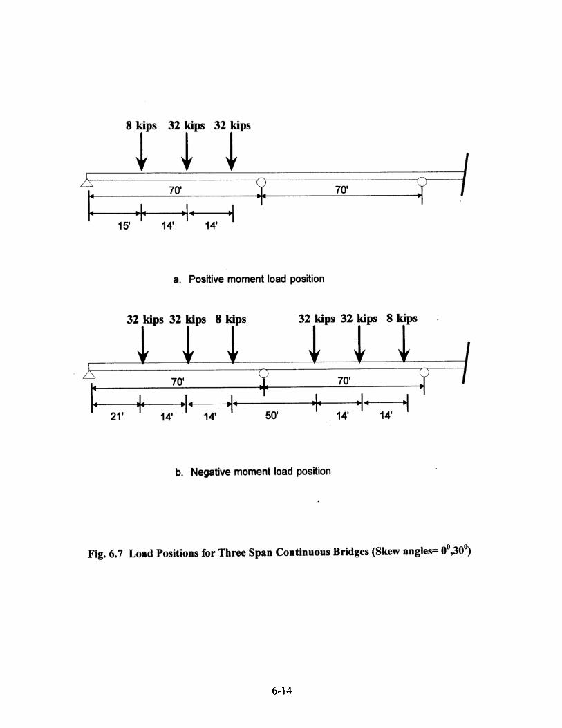
6.3.3 Parametric Studies The parametric study is focused on three main parameters: variation of skew angle, variation in

the number of spans, and change in the ratio between two spans. A total of 64 cases have been

investigated in this parametric study. The first section studies the effects of changing the skew

angle for a two-span continuous bridge. Each of these bridges with different skew angles have

four truck loading positions for obtaining the positive and negative moment distribution for

interior and exterior girders.

The second section involves changing the number of equal spans with two different skew angles. Each bridge has four truck loading positions for obtaining the positive and negative moment distribution for interior and exterior girders.

The third section studies the effect of varying ratios between the spans for two different

skew angles. The four truck ,load positions are also considered in each case. The summary of

parametric study is presented in Table 6.2. The load distribution factors for each case are

calculated and presented in Table 6.3.

6-18

6.3.3.1 Skew angle

Skew angle is an important factor in bridge design. The LRFD code provides for adjusting

the load distribution factors for different skew angles. The code does not specify any

recommendations for continuous bridges with different skew angles. The results from FEM analysis

of the continuous bridges are compared with LRFD load distribution factors based on single span

bridges.

Equation 6.8 is used to calculate the distribution factor of the internal girder. When

calculating the distribution factor for exterior girders, the exterior girder strains replace the

maximum strains as follows:

Figure 6.11 shows that the strains decrease with increase in skew angles for interior

girders. The skew angle induces significant twisting moment in the girders and gives an uneven

transverse strain distribution. The distribution factors at midspan of interior girders are shown in

Figure 6.12. The distribution factors based on FEM analysis are smaller than those based on LRFD

code. The difference in the distribution factors range from 15% for a straight bridge to 21% for a

bridge with a skew angle of 60 degrees. The trends of the variations are, however, the same for

both LRFD and FEM methods. Figure 6.13 shows the transverse strain distribution at midspan for

exterior girder loading. In general, the strain decreases as the skew angle increases. Figure 6.14

shows no clear trend for the change of load distribution factor with an increase in skew angle.

6-20

There is limited information on calculating distribution factors for negative moments in

continuous bridges. Figure 6.15 shows the transverse strain distribution at the interior support

for a continuous two-span bridge with different skew angles. The positive and negative strains (

Figs. 6.11 and 6.15) decrease with an increase in skew angles. Figure 6.16 shows the decrease

in distribution factors at the interior support for different skew angles. The rate of decrease in

the distribution factors based on FEM is less than that obtained using LRFD. This may be due to

the FEM idealization of the interior support as a knife edge, whereas, the interior support

reaction is distributed over a finite bearing width. This is also true in the case of negative

moment distribution factors for the exterior girders, as observed in Figs 6.17 and 6.18.

Based on the present studies on the effect of skew angles on continuous bridges, the following

observations are presented. The strains are higher at the interior supports than at midspans. The

higher strains at the interior support are the result of loading both spans with a total of 8 trucks;

four loaded in each span. The strains at midspan are due to only one span loaded with four

trucks. The strain .distributions are similar for both positive and negative moment loading. The

FEM distribution factors vary with different skew angles.

6.3.3.2 Number of spans

The effect of the number of spans on the distribution factor calculation is evaluated in this

section. The study cases are divided into two sets: straight bridges, and skewed bridges with an

angle of thirty degrees. Each set has two, three, and four spans for parametric variation. Figures

6.6, 6.7, and 6.8 show the truck load position for positive and negative moments.

Figure 6.20 shows the interior girder distribution factor variation with different number of spans

for straight bridges at the midspan. The FEM distribution factors are lower than the LRFD

factors and show no variation with an increase in the number of spans. Figure 6.22 shows a

small increase ( 9%) in the exterior girder load distribution factor as the number of spans

increase. For a skewed bridge at midspan, the interior girder distribution factor exhibits a small

decrease ( 13% ) with an increase in the number of spans ( Figure 6.24 ). The exterior girder

load distribution factor has small variations of less than 5% and can be neglected ( Figure 6.26 ).

Figures 6.28 and 6.30 show the interior and exterior girder distribution factors for a straight

bridge at the interior support. Little variation (3%) is observed with an increase in the number of

spans. Similar marginal variations are observed for the thirty degree skew bridge cases shown in

Figure 6.32 and 6.34.

In general, the FEM load distribution factors are smaller than those based on LRFD code. Based

on the parametric study, the effect of the number of spans on the load distribution factors can be

neglected. This conclusion is in agreement with LRFD code.

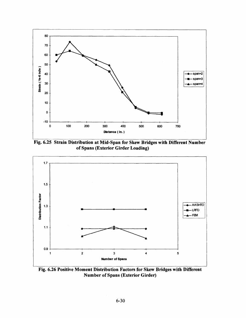
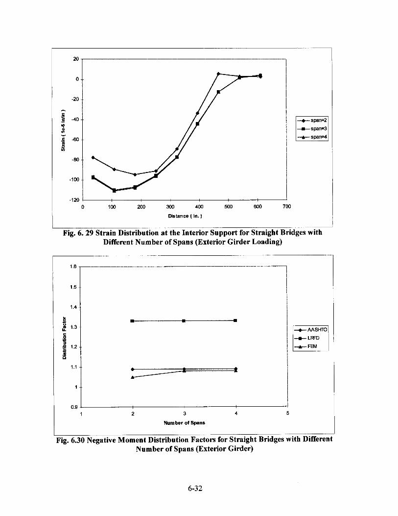
6.3.3.3 Ratios Between the Spans

The ratios between the spans for two span continuous bridges were varied to study the

effects on the load distribution factors. The ratios of the spans used in this study were 1:1, 1:1.5,

and 1:2. Bridges with thirty degree skew angle and straight bridges were used in this study. Figures

6.6, 6.9, and 6.10 show the truck load positions for maximum positive and negative moments in the

bridges with different ratios between spans. For the cases with the span ratios of 1:1.5 and 1:2, the

bridge was loaded for positive moment in each of the two spans.

Figure 6.36 shows the interior girder load distribution factor of a straight bridge at

midspan. Little variation in the load distribution factor is observed with increased ratios between

the spans. Figure 6.38 shows that the shorter span has a smaller increase (7%) in distribution

factor than the larger span ( 17%). The interior girder load distribution factors of a straight bridge

at the interior support are shown in Figure 6.40. Little variation was observed in the negative

moment load distribution factors. Similar behavior was observed in the interior girder positive

moment distribution factors. Figure 6.42 shows a slight increase ( 12%) in the exterior girder load

distribution factors at the interior support as the ratios increase between the spans.

The bridge with a thirty degree skew angle shows a decrease in the interior girder load

distribution factor at midspan with an increase in the ratios between the spans ( Figure 6.44).

Figure 6.46 shows the exterior girder load distribution factors at the midspan. The distribution

factors increase ( 11%) as the ratios between the spans increase.Figure 6.48 shows a little variation

in the interior girder load distribution factor at the support. The exterior girder

6-171

distribution factors show a slight increase ( 11 %) with increases in the ratios between the spans Figure 6.50).

In general, the interior girder load distribution factors show little variation as the ratios between the spans increase for both positive and negative moments. The exterior girder load distribution factors show a general increase (10%-13%) as the ratios between the spans increase.

6-172

6-40

6.4 FIELD TESTS ON CONTINUOUS SLAB-ON-GIRDER BRIDGES

There is an increase in the number of existing highway bridges which need to be evaluated

to permit increase in the live loads or for bridge strength determination taking into account

deterioration. The evaluation of Florida highway bridges is being conducted by The Florida

Department of Transportation Structures Research Center using non-destructive load tests. Load

testing provides a realistic evaluation of the bridge and load ratings that are essential for

determining safe service loads in the bridges. These ratings are based on the measured strains and

deflections due to the applied loads. The wheel load distribution factors are calculated based on

the field measurements.

Comparison between strain and deflection measurements of bridges with analytical values gives a perspective of the accuracy of the FEM to analyze the bridge behavior. The accuracy of FEM is dependent on the realistic modeling of the bridge and its boundary conditions. Three bridges tested by Florida Department of Transportation (FDOT) were analyzed using ANSYS finite element program. Of the three continuous bridges studied, two bridges are continuous through the deck slab and one bridge is continuous through the girder and the deck slab. The FDOT Eau Gallie Bridge was made continuous by post-tensioning the girders at the supports. The negative moment measurement showed that this bridge was truly continuous and is, therefore, used as a typical bridge in the parametric analysis of continuous bridges ( Section 6.3).

6-182

Field measurements from load tests by MOT and analytical results based on FEM models

are used to study wheel load distribution factors for continuous bridges. The FEM models for

continuous slab-on-girder bridges are shown in Figs 6.2 and 6.4.

6.4.1 SR-518 Eau Gallie Bridge

The Eau Gallie bridge is located in Melbourne, Florida, and is owned and operated by the

FDOT. The structure has spans ranging from 20 to 145 feet. The 7.5 in. thick deck is supported by

nine Bulb-T girders placed at 10'-4" center to center. The Bulb-T girders are made continuous by

post-tensioning. The deck is 90'-7.5" wide and has six traffic lanes with a 5 ft. pedestrian sidewalk.

The live load was applied with two 204 kip testing vehicles. Several load positions were performed

to study the effects of shear, maximum bending and twisting moments. The truck load positions are

shown in Figures 6.54 to 6.56.

First, the bridge was discretized to be continuous in the deck slab over the interior support with

restraint on the translational degrees of freedom at the end supports. In the second idealization, the

model was modified by making the girders continuous over the interior support. The analytical

results from the second modeling were found to give a reasonable correlation with the field test

values. Therefore, this model was chosen as a basis for the parametric study presented in this

chapter.

6-183

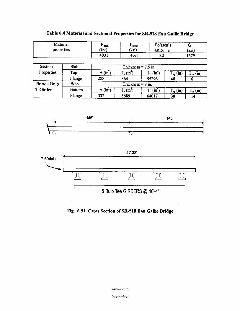
Span 1 Span 2

CL CL CL

i

I I I

- I o 30 mulmm o m m 6' I o ~~ o

12.75' I

I L _I. ,

51.5' 66.5'

a. Load Position 1

Span 1 Span 2

CL CL CL

I

I

I

I

I

. / • 12.75'

I

I 51.5'

I 66.5'

b. Load Position 2

LVDT on Girder FEW 26.16 kips

STRAIN GUAGE

20.93 kips

on Girder 7.82 kips

Fig. 6.54 Load Positions 1 and 2/Strain Gauges SR-518 Eau Gallie Bridge

6-50

The truck load positions 1 and 2 induce maximum positive moments in the two spans ( Fig 6.54 ). Load position 2 has the same loading configuration as load position 1 with the trucks advanced forward to span 2. The positioning of the trucks for the third load case was chosen to give maximum twisting moment. Truck load position 4 has two trucks loaded on span 2 to produce maximum deflection. Truck load position 5 is similar to position 4 with the trucks loaded on span l. Figure 6.57 shows the deflection distribution on the loaded span at the midspan for load position 1. The maximum deflection based on FEM is within 10% of the measured maximum deflection. The exterior girders' deflections were less accurately predicted. Figure 6.58 shows the deflection distribution on the unloaded span at the midspan for load position 1. The deflections are predicted accurately using FEM. Figure 6.59 shows the deflection distribution on the unloaded

span at the midspan for load position 2. There is a small difference between the field tests and the FEM prediction. Figure 6.60 shows the deflection distribution on the loaded span at the midspan for load position 2. The measured deflections were supposed to be similar to those for load position 1, however, a significant difference has been observed in the reported data. The FEM deflections were similar for positions 1 and 2. The deflection variations at midsection of span 1 and 2 for load position 3 are shown in Figures 6.61 and 6.62. Figure 6.63 and 6.64 show the deflection variations at the midsections of the loaded and unloaded spans, respectively, for load position 4. For load position 5, the deflection distributions at midsections for unloaded and loaded spans are shown, respectively, in Figures 6.65 and 6.66. In all of the above cases, it can be observed that the differences between the measured and the analytical values are relatively small.

6-53

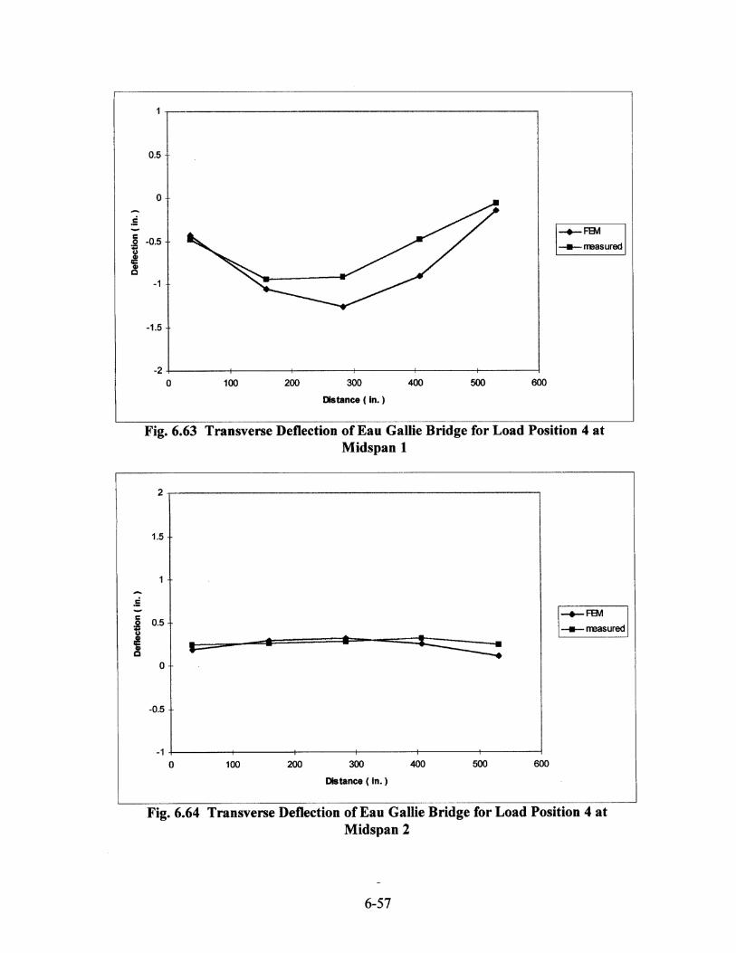
Table 6.5 summarizes the load distribution factors for the Eau Gallie bridge based on AASHTO, LRFD, FEM, and field tests. The distribution factors based on AASHTO and LRFD are larger than those based on the measured deflections and FEM. Load position 4 at span 1 gives the maximum load distribution factor for the field tests and FEM. These factors are lower than the LRFD factor by 16%. The maximum load distribution factor for span 2 corresponds to load position 5. The FEM and measured factors are lower that AASHTO and LRFD distribution factors. The FEM load distribution factors are close to the factors based on the field tests. Therefore, the finite element method should be used for the analysis of existing continuous slab-ongirder bridges.

6.4.2 SR-55 Bridge Over Suwannee River

The bridge is located on SR-55 over the Suwannee River at Fanning Springs, Florida. The bridge has two 121'-3" spans made continuous through the deck slab and a simple 66' span. The 42'-9" wide 7 in. thick deck slab is supported by eight AASHTO IV girders spaced at 4'-11.5" centers.

The bridge was loaded with two FDOT test vehicles. The bridge was modeled as continuous

through the deck slab at the interior support with discontinuous girders at the interior support.

The ends of the bridge were restrained against translational degrees of freedom and the bottom

of the girders at the interior support of the bridge were constrained in the vertical and transverse

directions. Figure 6.69 shows the truck load position and the strain gauge location in span

2 of the SR-55 bridge. The field measurements were taken for three different loads ( 100, 152

and 204 kips ) for this truck load position.

6-61

The measured strains for the different loads on the SR-55 Bridge Over Suwannee River are slightly higher than the analytical values ( Fig 6.70). The transverse strain distributions from the measured and analytical values are similar for each of the applied loads. The measured and computed strains compare well in the girders where the trucks are loaded and the girder strains vary only slightly as the girder distance from the trucks increase ( Fig 6.70 and Table 6.7).

6-200

Table 6.8 shows small differences in the load distribution factors obtained from the

measured and FEM strain values. The AASHTO and LRFD load distribution factors are higher

than the FEM and measured distribution factors.

6.4.3 Palm Beach County Bridge #930398

The bridge is located in Palm Beach County on Hoods Road over I-95. It has four spans,

two of which are continuous. The intermediate continuous spans are 143'-7 3/16" long and 46'-9"

wide. The 7 in. thick deck slab is supported on six AASHTO V girders at T-9.5" centers.

The bridge is modeled as continuous through the deck slab at the interior support with all

end translations restrained. The bridge's six diaphragms were modeled using shell elements ( shell

63) in the transverse direction. Two of the diaphragms are located at the interior support and the

other four diaphragms are located at third points of each span. The ends of the bridge were

restrained against the translational degrees of freedom and the bottom of the girders at the interior

support of the bridge were constrained in the vertical and transverse directions. Figure 6.74 shows

6-202

the truck load position in span 1 of the Palm Beach County Bridge. The field measurements were taken for a truck load of 140 kips.

The measured transverse strains in the bottom of the girders in Bridge #930398 compare closely with FEM values. The strains in the girders, where the trucks are positioned, agree well with the measured values (Fig. 6.75). The AASHTO and LRFD distribution factors are higher than the measured and FEM values. The measured distribution factor is slightly lower than the FEM results (Fig. 6.10).

6-69

6-70

CHAPTER 7

SUMMARY AND

CONCLUSIONS 7.1 SUMMARY The present study on wheel load distribution is focused on the skew slab-on-girder and skew solid slab

bridges. Chapter 2 reviews the existing different analytical and field load distribution methods for different

skew bridge types. Chapter 3 discusses the concepts of the finite element method in bridge modeling and

idealization, field test procedures and methodologies.

Both analytical and field studies on the truck load distribution of skew simply supported slab-on-girder

bridges are presented in Chapter 4. Finite element method is used to study the various parameters affecting

load distribution and suggest which parameters must be considered ( 70 study cases were performed). In

addition to the analytical study, data from field tests performed by Structures Research Center, FDOT, are used

to verify the analytical results.

In Chapter 5, both analytical and field studies on the wheel load distribution of skew simply supported

solid slab bridges are presented. Finite element method is used as an analytical tool to study the various

parameters affecting load distribution and suggest which parameters should be considered. In addition to the

analytical study, data from field tests performed by Structures Research Center, FDOT, are compared with

those based on the finite element, AASHTO and LRFD codes. Several parameters such as skew angle, span

length, bridge width, slab thickness, edge beam and number of lanes are considered in the parametric studies.

7-1

In Chapter 6, finite element method is used to analyze continuous skew and striate slab-on-I

girder bridges and calculate the corresponding load distribution factors. The analytical results obtained are

compared with those based on AASHTO (1989) and the LRFD (1995) codes. Field test data of continuous

bridges are analyzed to investigate the load distribution factors.

7.2 CONCLUSIONS 7.2.1

Skew Solid Slab

Bridges i) The effective widths calculated using finite element method are larger than those calculated using

AASHTO and LRFD codes, which indicate that both AASHTO and LRFD codes give conservative

estimate of effective width, E for skew solid slab bridges.

ii) The effective width increases with increase in the skew angle for solid slab bridges. This confirms the

LRFD codes in considering the skew angle as a parameter in effective width calculation. The finite

element results show smaller skew angle effects than those in LRFD codes except for skew angle

higher than 45 degrees where the effects are the same as in the LRFD code.

iii) The span length is an important factor in effective width calculation. The effective width tends to increase as the span length increases. The span length effects on the effective width calculation are the same from finite element analyses, AASHTO, and LRFD codes. iv) The edge beam moment increases with increase in moment of inertia, i.e. increase in edge beam depth or width. The edge beam depth significantly affects the value of effective width, E. Slab bridges without edge beams or with hidden edge beams have greater maximum moment than similar slab bridges with

7-209

edge beams or with hidden edge beams have greater maximum moment than similar slab bridges with

edge beam and hence the resulting effective width is smaller. These results suggest that the edge beam

size should be taken into account in wheel load distribution. Neither AASHTO specifications nor the

LRFD code considers the edge beam effect in the effective width equation.

v) Based on the skew solid slab parametric studies, the skew angle, span length and the edge beam depth are the main parameters, which significantly affect the effective width calculations. Effective width equations are proposed for solid slab skew bridges without edge beams and with edge beams. vi) Effective widths calculated from finite element method and measured strains are higher than the AASHTO

and LRFD values. The effective widths based on the AASHTO and LRFD codes are more conservative.

7.2.2 Skew Slab-on-Girder Bridges

i) Skew angle increase reduces load distribution for the interior girders. Considering the finite element

results, it seems that the LRFD code accurately estimates the skew angle effect particularly for skew

angles higher than 30 degrees.

ii) Skew angle effect on load distribution for exterior girders is similar to that of the interior girders. The finite

element results show decrease in the load distribution factor with the increase in skew angles. These

results confirm those based on the LRFD code where the load distribution factors decreases with the

increase in the skew angle.

iii) Girder spacing is a very important factor in determining flexural wheel load distributions of skew slabon-

girder bridges.

7-210

iii) Girder spacing is a very important factor in determining flexural wheel load distributions of skew

slabon-girder bridges.

iv) The flexural distribution factors based on LRFD are slightly smaller than those calculated using

finite element method particularly for larger girder spacing. It is shown that the distribution factors

based on LRFD code are in better agreement with those calculated using finite element method for

smaller girder spacings which are more commonly used.

v) The interior girder distribution factor calculated using finite element method shows much smaller

decrease with increasing span length than those based on LRFD code. However, the load distribution

for exterior girders based on finite element analyses and LRFD codes shows conflicting results.

vi) For a given skew angle, girder spacing and span length, the LRFD load distribution equation

overestimates the effect of slab thickness on wheel load distribution. The finite element results show no

or little effect on load distribution for variation of slab thicknesses between 3.85 in to 7 in. which

corresponding variation of H between 5 and 30. (H = stiffness ratio = Eg Iv, / a D , D = flexural stiffness

of slab per unit width)

vii) The data from three field tests conducted on skew slab on I-girder bridges in Duval county, State

Road 7 and Turnpike were used to validate the finite element model. In addition these field tests were

used to calculate the wheel load distribution factors based on measured strains, finite element

analyses, AASHTO and LRFD codes.

viii) The load distribution factors based on finite element analyses were the most close to those based on

the measured strains (less than 30 % difference). This difference may be attributed to the variations

in 7-4

concrete strength and section modulus, which are used in calculating the measured DF. Both DFs

based on AASHTO and LRFD were higher than those calculated using the measured strains and

finite element method. This confirms that AASHTO code and to a lesser extent, the LRFD code

give conservative values for wheel load distribution factor for skew slab-on-girder bridges.

7.2.3 Continuous Slab-on-Girder Bridges

7.2.3.1 Field Tests From this study of wheel load distribution factors on continuous highway bridges, there exists a

need to use computer modeling to accurately predict the behavior of existing bridges. Finite element

analysis of continuous bridges has shown that the AASHTO and LRFD codes' wheel load distribution

factors are conservative. The conservative approach may be needed in the design of highway bridges.

However, rating of existing bridges for load capacity should be based on more accurate methods.

7.2.3.2 Parametric Study

The parametric study of continuous bridges investigated the effects of number of spans, the skew

angle, and the ratio between two spans.

i) Changing the skew angle generates strains which are higher at the interior supports than at

midspans. The strains at midspan are due to one span loaded with four trucks. The higher

strains at the interior support are the result of loading both spans with a total of 8 trucks;

four loaded in each span. The strain distributions are similar for both positive and negative

moment loading. The FEM analyses show strain distributions become less uniform as skew

angle increases.

7-212

Based on this parametric study, the effect of the number of spans on the load distribution factors is small and can be neglected. In general, the FEM load distribution factors are smaller than those based on LRFD code. In general, the interior girder load distribution factors show little variation as the ratios between the spans increase for both positive and negative moments. However, the exterior girder load distribution factors show a general increase (10%-13%) as the ratios between the spans increase.

7-213