Embed Size (px)
Citation preview
2
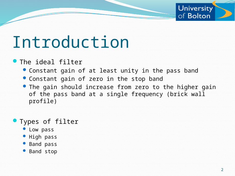
IntroductionThe ideal filter
Constant gain of at least unity in the pass band Constant gain of zero in the stop band The gain should increase from zero to the higher gain of the pass band at
a single frequency (brick wall profile)
Types of filter Low pass High pass Band pass Band stop
3
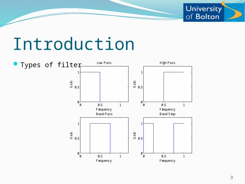
IntroductionTypes of filter
0 0.5 10
0.5
1
Low Pass
Gai
n
Frequency0 0.5 1
0
0.5
1
High Pass
Gai
n
Frequency
0 0.5 10
0.5
1
Band Pass
Gai
n
Frequency0 0.5 1
0
0.5
1
Band Stop
Gai
n
Frequency

4
Introduction Digital filters can be divided broadly into two types:
Finite Impulse Response – FIR
Infinite Impulse Response – IIR
FIR filters are never unstable and have a linear phase response
IIR require fewer coefficients to achieve the same magnitude frequency response.
The two types of filter are very different in their performance and design

5
IIR Filter Design MethodsDirect Design – pole-zero placement
Bilinear Transform Method
Impulse Invariant Method
Pole-zero Mapping Method

6
Pole-zero Placement Poles and zeros are placed on the z-plane to try and achieve the
required frequency response.
Often an element of trial and error is involved
Tweaking can be small in trying to fine tune the filter response, tools like Matlab can speed up this process.
Once the map is obtained we can then easily Obtain the system transfer function Convert the transfer function into a practical implementation
7
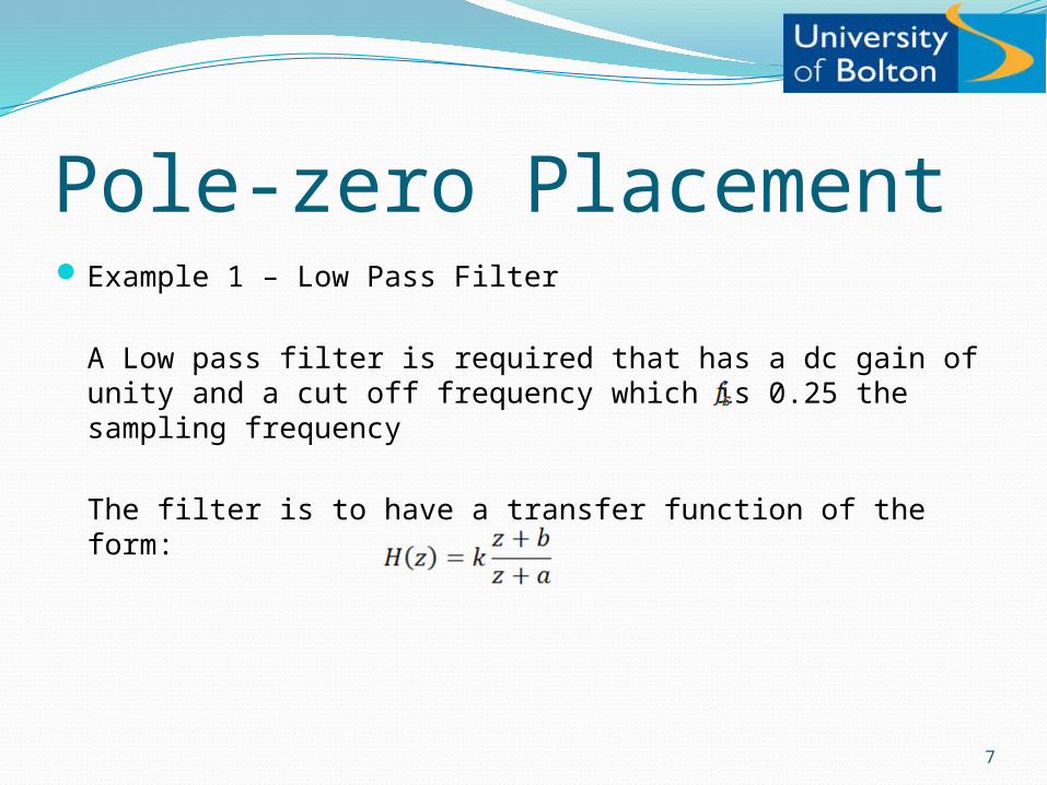
Pole-zero Placement Example 1 – Low Pass Filter
A Low pass filter is required that has a dc gain of unity and a cut off frequency which is 0.25 the sampling frequency
The filter is to have a transfer function of the form:
8
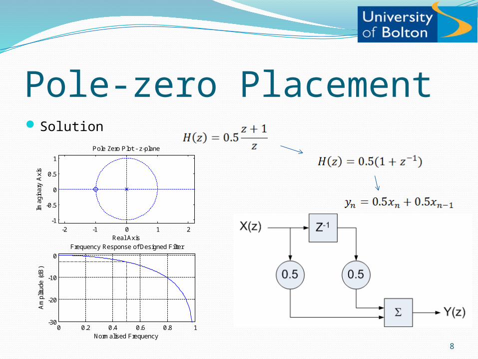
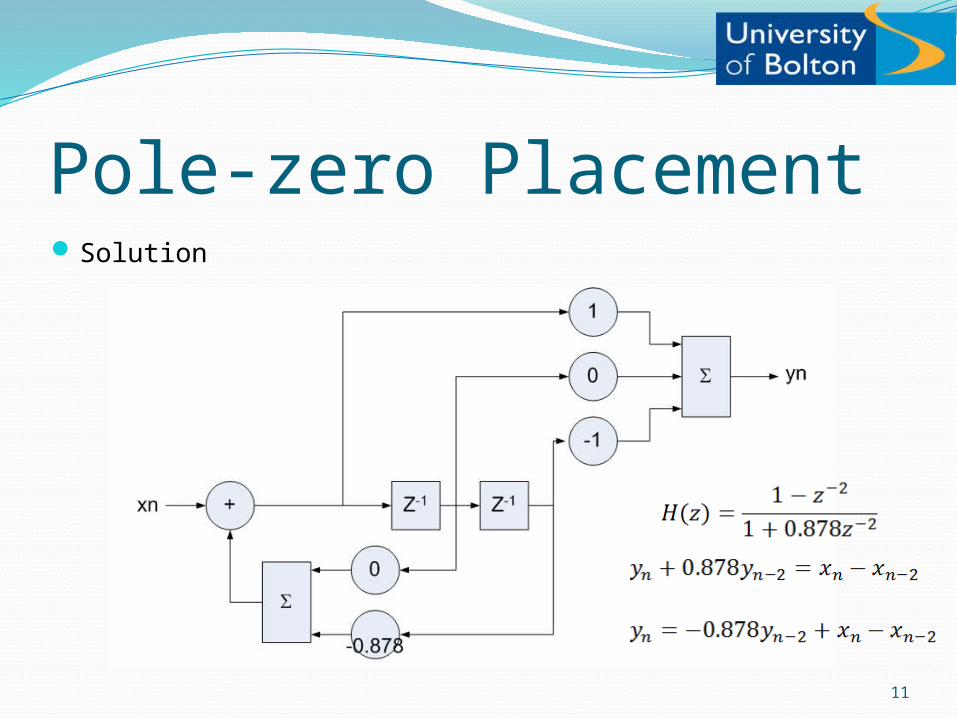
Pole-zero Placement Solution
-2 -1 0 1 2-1
-0.5
0
0.5
1
Real Axis
Imag
inar
y A
xis
Pole Zero Plot - z-plane
0 0.2 0.4 0.6 0.8 1-30
-20
-10
0
Am
plitu
de (
dB)
Normalised Frequency
Frequency Response of Designed Filter

9
Pole-zero Placement Example 2 – Band Pass Filter
A band pass filter is required to meet the following specification
Complete signal rejection at dc and 500Hz A narrow pass band centred at 250Hz A 3dB bandwidth of 20Hz
Assume a sampling frequency of 1000Hz
a) Find the transfer function using the zero pole placement method
b) Find the difference equation
c) Propose a diagrammatical solution
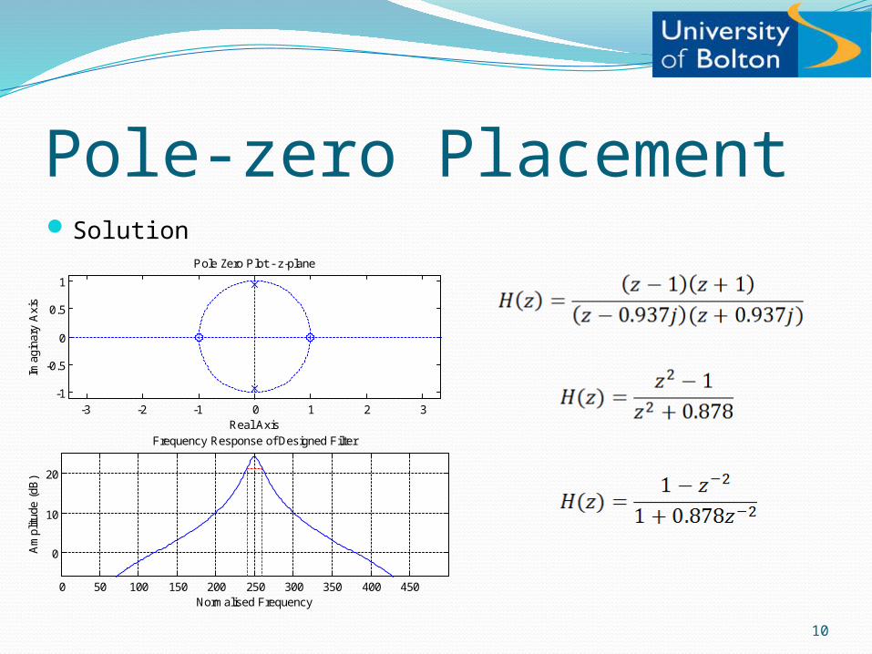
10
Pole-zero Placement Solution
-3 -2 -1 0 1 2 3-1
-0.5
0
0.5
1
Real Axis
Imag
inar
y A
xis
Pole Zero Plot - z-plane
0 50 100 150 200 250 300 350 400 450
0
10
20
Am
plitu
de (
dB)
Normalised Frequency
Frequency Response of Designed Filter

12
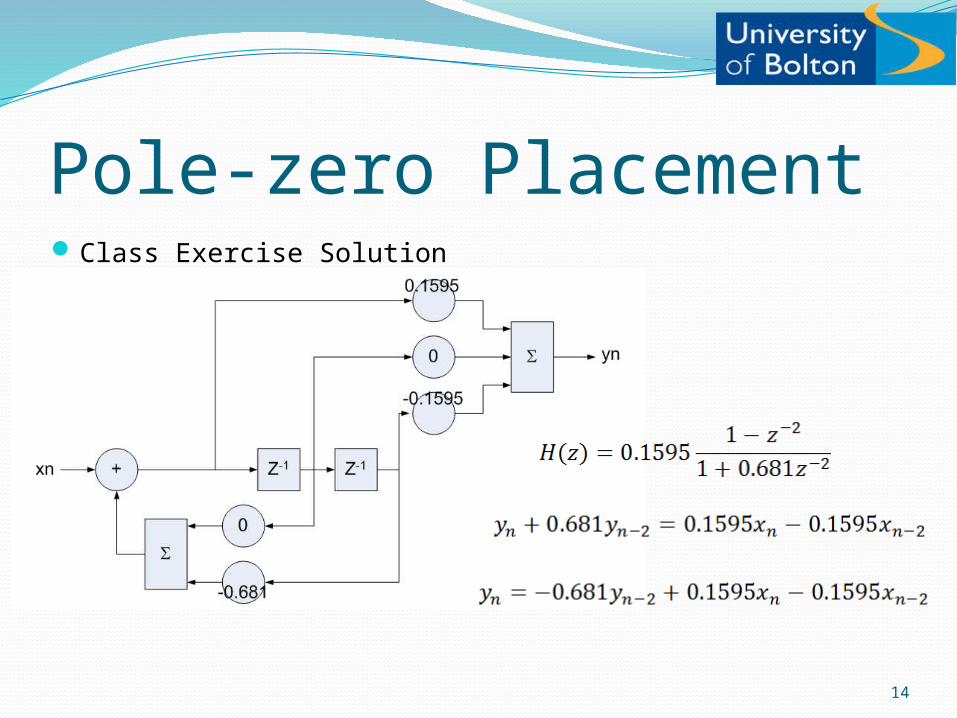
Pole-zero Placement Class Exercise
An analogue signal has a spectrum that extends from dc to 9kHz. It is required to extract a particular frequency component at 2.25kHz.
Using pole zero placement, design a band-pass filter that has the centre of its pass-band at 2.25kHz and a zero in its frequency response at dc and at 4.5kHz. Additionally, the filter magnitude response should be unity at 2.25kHz and at 2kHz.
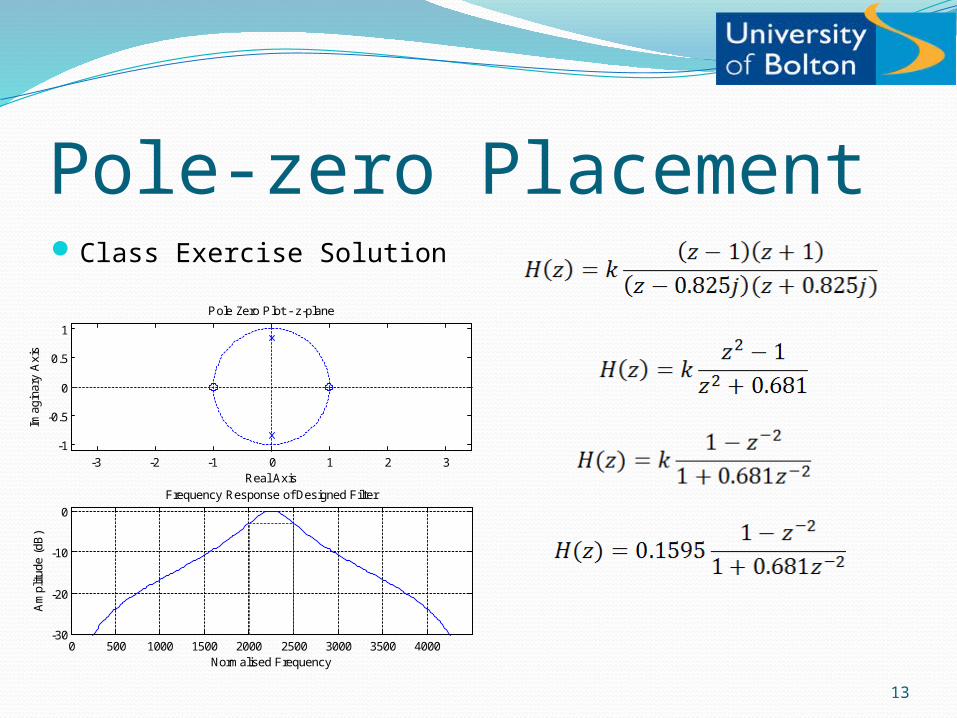
13
Pole-zero Placement Class Exercise Solution
-3 -2 -1 0 1 2 3-1
-0.5
0
0.5
1
Real Axis
Imag
inar
y A
xis
Pole Zero Plot - z-plane
0 500 1000 1500 2000 2500 3000 3500 4000-30
-20
-10
0
Am
plitu
de (
dB)
Normalised Frequency
Frequency Response of Designed Filter
15
IIR Filter Design using Analogue Filter Templates Pole zero placement is adequate for fairly simple designs Complex designs need an alternative approach There is a vast knowledge base of the design of analogue filters
Butterworth Chebyshev
Mathematical techniques have been developed to convert a filter described in the s-domain to that described in the z-domain
These designs result in an approximation to the analogue design but an exact match is impossible…..a digital filter is not expected to operate above the Nyquist frequency
Three techniques covered here Bilinear Transform Impulse Invariant Transform Pole-zero matching

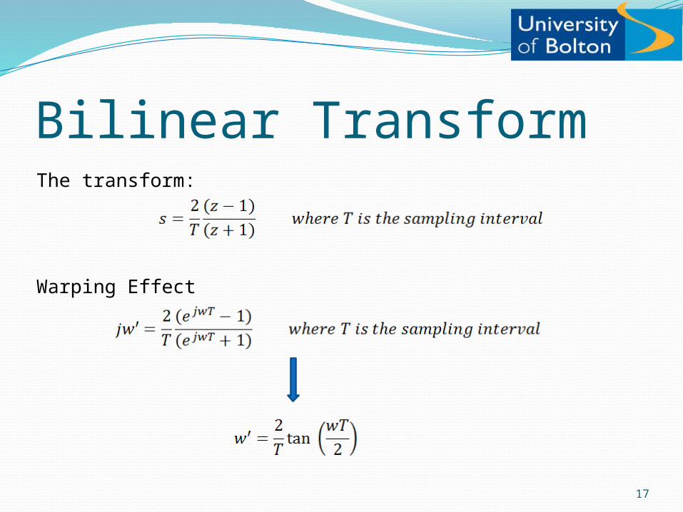
16
Bilinear TransformThe transform:
Example:
Consider a first order low pass analogue filter having a cut off frequency at 10 rads/s

18
Bilinear TransformA change in sampling frequency will affect the problem of warping
(try increasing the sampling frequency by a factor of 10 and then recalculate w’ for the previous example)
Pre-warping only ensures that the gain is matched at the chosen frequency and 0Hz
It the design has several break points then a decision has to be made as to which one to preserve
It there is a difference of more than 1% between w and w’ then pre-warping is advised
19
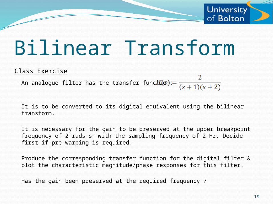
Bilinear TransformClass Exercise
An analogue filter has the transfer function:
It is to be converted to its digital equivalent using the bilinear transform.
It is necessary for the gain to be preserved at the upper breakpoint frequency of 2 rads s-1 with the sampling frequency of 2 Hz. Decide first if pre-warping is required.
Produce the corresponding transfer function for the digital filter & plot the characteristic magnitude/phase responses for this filter.
Has the gain been preserved at the required frequency ?
20
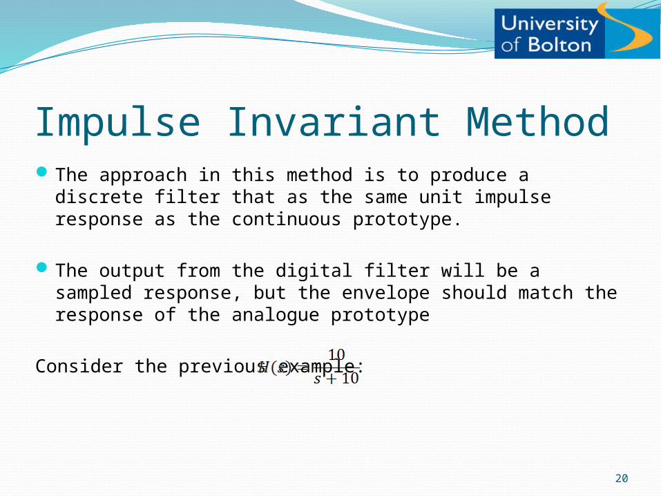
Impulse Invariant MethodThe approach in this method is to produce a discrete filter that as the
same unit impulse response as the continuous prototype.
The output from the digital filter will be a sampled response, but the envelope should match the response of the analogue prototype
Consider the previous example:

21
Impulse Invariant MethodComparison between the analogue prototype and the digital
representation from the IIT method
This normalised digital filter gives a comparable magnitude response to the analogue prototype at low frequency but the discrepancy grows as the Nyquist frequency is approached.
Ideally the signal should be sampled at a frequency which is much higher than the desired cut-off frequency. In this example, the sampling is at a factor x10 of the desired cut-off frequency i.e. Fs=16 Hz with fc=1.6 Hz.

22
Impulse Invariant MethodClass Exercise
An analogue prototype has a transfer function given by:
Convert this to its discrete normalised equivalent using the Impulse Invariant method using a sampling frequency of 20 Hz.
Produce & compare the impulse responses of the two filters & produce & compare the corresponding frequency responses.
23
Pole-Zero Mapping Method This approach uses the relationship to convert the s-plane
singularities (poles & zeros) of the CT prototype filter to equivalent z-plane singularities.
Once these have been determined, then the corresponding transfer function
can be constructed to describe the digital design.
All that needs to be done further is to match the gain at some appropriate frequency (often 0 Hz).
24
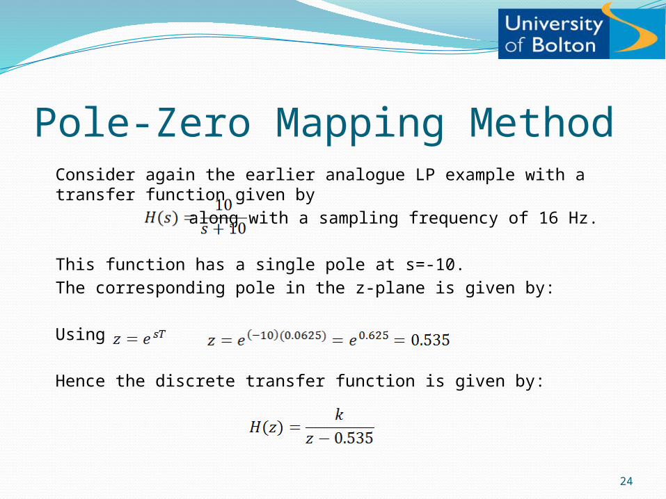
Pole-Zero Mapping MethodConsider again the earlier analogue LP example with a transfer function given by
along with a sampling frequency of 16 Hz.
This function has a single pole at s=-10.
The corresponding pole in the z-plane is given by:
Using
Hence the discrete transfer function is given by:


![Dual Variable Gain Duplex Filter[1]](https://img.pdfslide.us/doc/110x75/552df772550346231a8b4832/dual-variable-gain-duplex-filter1.jpg)