Unit 8: Gravitational and electric forces and fields

1 The story of planetary motion

On what do we base our scientific theories? When we look up at the sky, how have we learned what we know about the

motion of the planets? The understanding of the phenomena of the physical world usually follows from observation and

successive attempts at explanation, frequently spread over a period of time and with many setbacks on the way. A very

interesting example of this is the explanation of the motion of the planets.

The movement of celestial bodies had, of course, been noted over thousands of years, the planets being distinguished

mainly by their relatively rapid motion in the night sky. In fact, the word planet is derived from the Greek word for

wanderer. This motion is illustrated in Figure 1.

View larger imageFigure 1 The night sky, showing the track of

the planet Mars over a period of about nine months.

In the ancient world, the Earth was accepted as the centre of the Universe, and the model proposed by the Greek

astronomer Claudius Ptolemy in the second century AD was the accepted theory for the next 14 centuries. However, in

1543, the Polish astronomer Nicolaus Copernicus (1473–1543) proposed that the Earth executed a circular orbit centred

on the Sun — a heliocentric model replacing a geocentric model. This now relegated the Earth to the same status as the

other planets, which were also held to be orbiting about the Sun. This hypothesis was most certainly not welcomed and

was subjected both to ridicule and suppression. This is not uncommon with the breaking of totally new theoretical ground.

The next stage in the story arose from accurate measurement (accurate, of course, in the context of that era). Over a

period of more than 30 years, using a sextant and compass, the Danish astronomer Tycho Brahe (1546–1601) made

accurate measurements of all the astronomical objects he could see with the naked eye in the night sky (the telescope

had not been invented). His successor, the German astronomer Johannes Kepler (1571–1630), analysed Tycho’s

measurements and, after laborious calculations extending over about fifteen years, discovered that the observations,

initially for Mars but later for the other known planets, could be explained by a heliocentric motion that followed three

laws. The first of these empirical laws required the motion to be not circular but elliptical, with the Sun at one focus of the

ellipse (see Figure 2).

Figure 2 (a) The Copernican circular motion of the Earth. (b) The

Keplerian elliptical motion of the Earth. (Neither diagram to scale.)

Figure 3 (a) Tycho Brahe (1546–1601); (b) Johannes Kepler

(1571–1630); (c) the platonic spacing of planetary orbits, according

to Kepler.

Show transcriptDownloadAudio 1 Tycho and Kepler

Did this settle any arguments? Unfortunately, it did not. Kepler’s three laws were empirical, and although his first law

fitted the observations, so did Ptolemy’s conceptions. In the Greek world, the circle was the perfect geometrical figure. If

the motion of a planet was not circular, then it might be made up of a circle imposed on another circle — an epicycle — or

a circle imposed on a circle imposed on a circle, and so on. If there were no rules about the number of epicycles or their

radii, the Ptolemaic method could explain the observations just as accurately — but certainly not as simply — as the

Keplerian ellipses. (It is difficult to appreciate how strong was the attachment to the circle as the perfect geometrical

figure. Even Galileo wanted to stick to circles.) About a hundred years later, Isaac Newton (1642–1727) demonstrated

that the Keplerian ellipses arose as a consequence of combining his laws of motion with a simple force law for

gravitation. The resolution of the conflict between the two systems is the subject of the next section.

2 Gravitational forces and fields

2.1 Newton’s law and gravitational forces between two masses

In earlier Units, you learned about Newton’s three laws of motion and how they may be applied to predict the motion of

bodies under the influence of specified forces. Amongst his many other great achievements, Isaac Newton (Figure 4)

also proposed the law of universal gravitation. He graduated from the University of Cambridge, England in 1665, but, due

to an outbreak of plague, he spent the next 18 months at his home in Woolsthorpe in Lincolnshire. In this time, which he

regarded as his prime, he invented integral and differential calculus and discovered the law of universal gravitation.

However, on his return to Cambridge when the University reopened in 1667, due to his secretive nature, he revealed little

of his achievements. It was not until later that he was persuaded to collect his ideas on mechanics into a book, the

Principia Mathematica, which was published in 1687. This contained, amongst other things, the formulation of his now

well-known three laws of motion and their application using his universal law of gravitation to derive Kepler’s three laws.

Characteristically, his derivations were geometrical rather than based on his calculus, doubtless to avoid controversy

about the validity of his new form of mathematics.

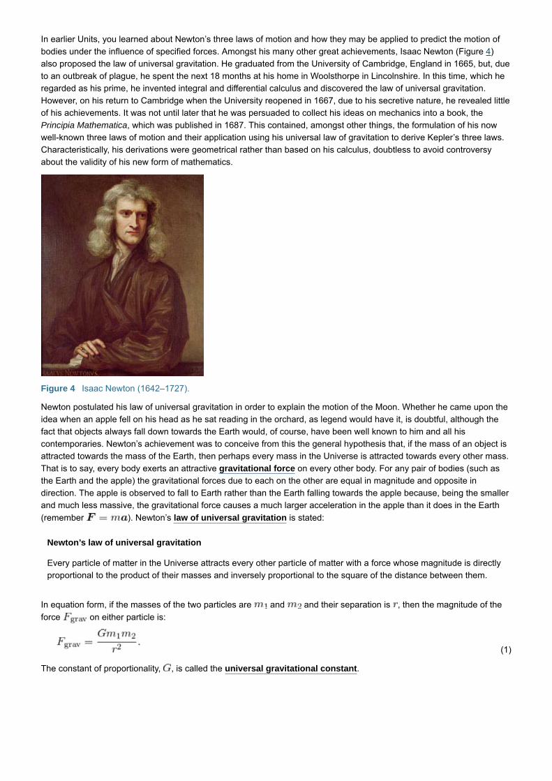
Figure 4 Isaac Newton (1642–1727).

Newton postulated his law of universal gravitation in order to explain the motion of the Moon. Whether he came upon the

idea when an apple fell on his head as he sat reading in the orchard, as legend would have it, is doubtful, although the

fact that objects always fall down towards the Earth would, of course, have been well known to him and all his

contemporaries. Newton’s achievement was to conceive from this the general hypothesis that, if the mass of an object is

attracted towards the mass of the Earth, then perhaps every mass in the Universe is attracted towards every other mass.

That is to say, every body exerts an attractive gravitational force on every other body. For any pair of bodies (such as

the Earth and the apple) the gravitational forces due to each on the other are equal in magnitude and opposite in

direction. The apple is observed to fall to Earth rather than the Earth falling towards the apple because, being the smaller

and much less massive, the gravitational force causes a much larger acceleration in the apple than it does in the Earth

(remember ). Newton’s law of universal gravitation is stated:

Newton’s law of universal gravitation

Every particle of matter in the Universe attracts every other particle of matter with a force whose magnitude is directly

proportional to the product of their masses and inversely proportional to the square of the distance between them.

In equation form, if the masses of the two particles are and and their separation is , then the magnitude of the

force on either particle is:

The constant of proportionality, , is called the universal gravitational constant.

(1)

Figure 5 The gravitational forces exerted by two particles on

each other.

Because every body attracts every other body, then, for any pair of masses and the force on body due to

body must be in the opposite direction to the force on body due to body as shown in Figure 5. The figure

illustrates the fact that the gravitational force is a vector and . The vector is, in each case, along the line

joining the two bodies. Each force has the magnitude , as given by Equation 1.

2.2 The measurement of G and the mass of the Earth

The postulation of the ‘inverse square’ gravitational force allowed Newton to explain Kepler’s laws. (In addition, in the

Principia, he showed that, beyond its own surface, a spherically symmetric body exerts the same gravitational force on

another body as would a point particle of the same mass located at the centre of the sphere. This allows considerable

simplification in the mathematics.) However, the experimental study of the law and the measurement of the gravitational

constant was not accomplished for another century. This achievement was reported in a paper of 1798 by another

remarkable personality, the Hon. Henry Cavendish (1731–1810) (Figure 6). The value he obtained was very close to the

modern value: .

Exercise 1

Show that the unit of can also be written as .

Answer

The unit of force, the newton, can also be written as mass times acceleration, i.e. . Substituting this into

gives , which simplifies to .

Figure 6 Henry Cavendish was born into an aristocratic English

family. He inherited a large fortune and after leaving the University

of Cambridge (without a degree), he was able to devote the

remainder of his life exclusively to his scientific research which he

carried out at his home in London. He avoided contact with people

— especially women, to whom he would never speak — and was

motivated mainly by curiosity, publishing very little of his work. His

measurement of used the principle of the torsion balance

invented by his contemporary John Michell (1724–1793).

The experiment to measure will not be discussed here. The use of the torsion balance will be discussed in Section 4 of

this Unit in connection with the electrostatic force. The principle of the experiment is the same although, because of the

relative weakness of the gravitational force, the dimensions of the torsion bar and the difficulty of the experiment were

very different. Cavendish was the first person to estimate the mass of the Earth using the value of the constant he had

obtained and other information known at that time, namely the magnitude of the acceleration due to gravity at the surface

of the Earth, , and the radius of the Earth, . The reasoning is as follows:

Figure 7 A mass at the surface of a spherical Earth. The Earth

is shown ‘cut away’ to make it clear that the force is directed to the

centre of the Earth.

Consider a small object of mass at the surface of the Earth, as shown in Figure 7. The object will experience a

gravitational attraction toward the centre of the Earth and so be subject to a force of magnitude , given by

Equation 1. If the mass of the Earth is , then, using Newton’s result that, outside its radius, a sphere exerts the same

force as if all of its mass were concentrated at its centre, the magnitude of the force experienced by the object will be

Now, the gravitational force on the object is nothing other than the weight of the object, which has magnitude , so we

can write

where is the magnitude of the acceleration due to gravity at the surface of the Earth. Comparing this expression for

with Equation 2, we can cancel the and, after some rearrangement, obtain

So, substituting the known values for the constants on the right-hand side of Equation 4, we find

Exercise 2

Two small, highly dense, bodies, each of mass , are separated by a distance of .

(a) Calculate the gravitational force between them.

Answer

The magnitude of the gravitational force between two masses apart is found by substitution in

Equation 1:

(b) What proportion is this of the weight of either mass at the surface of the Earth?

Answer

The weight of either mass is given by:

The ratio is

2.3 Addition of forces: more than two masses

So far, we have considered only the gravitational force between two isolated point masses. However, if three or more

(2)

(3)

(4)

massive bodies are present, we can still use Equation 1 to calculate the forces between each pair of masses. To find the

resultant force acting on a particular mass, we can calculate the forces on it due to each of the other masses separately,

and then add them together.

Exercise 3

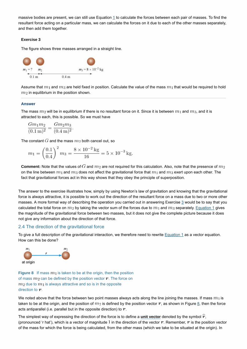
The figure shows three masses arranged in a straight line.

Assume that and are held fixed in position. Calculate the value of the mass that would be required to hold

in equilibrium in the position shown.

Answer

The mass will be in equilibrium if there is no resultant force on it. Since it is between and , and it is

attracted to each, this is possible. So we must have

The constant and the mass both cancel out, so

Comment: Note that the values of and are not required for this calculation. Also, note that the presence of

on the line between and does not affect the gravitational force that and exert upon each other. The

fact that gravitational forces act in this way shows that they obey the principle of superposition.

The answer to the exercise illustrates how, simply by using Newton’s law of gravitation and knowing that the gravitational

force is always attractive, it is possible to work out the direction of the resultant force on a mass due to two or more other

masses. A more formal way of describing the operation you carried out in answering Exercise 3 would be to say that you

calculated the total force on by taking the vector sum of the forces due to and separately. Equation 1 gives

the magnitude of the gravitational force between two masses, but it does not give the complete picture because it does

not give any information about the direction of that force.

2.4 The direction of the gravitational force

To give a full description of the gravitational interaction, we therefore need to rewrite Equation 1 as a vector equation.

How can this be done?

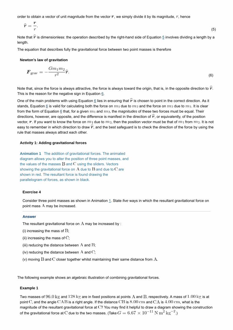
Figure 8 If mass is taken to be at the origin, then the position

of mass can be defined by the position vector . The force on

due to is always attractive and so is in the opposite

direction to .

We noted above that the force between two point masses always acts along the line joining the masses. If mass is

taken to be at the origin, and the position of is defined by the position vector , as shown in Figure 8, then the force

acts antiparallel (i.e. parallel but in the opposite direction) to .

The simplest way of expressing the direction of the force is to define a unit vector denoted by the symbol ,

(pronounced ‘r hat’), which is a vector of magnitude in the direction of the vector . Remember, is the position vector

of the mass for which the force is being calculated, from the other mass (which we take to be situated at the origin). In

order to obtain a vector of unit magnitude from the vector , we simply divide it by its magnitude, , hence

Note that is dimensionless: the operation described by the right-hand side of Equation 5 involves dividing a length by a

length.

The equation that describes fully the gravitational force between two point masses is therefore

Newton’s law of gravitation

Note that, since the force is always attractive, the force is always toward the origin, that is, in the opposite direction to .

This is the reason for the negative sign in Equation 6.

One of the main problems with using Equation 6 lies in ensuring that is chosen to point in the correct direction. As it

stands, Equation 6 is valid for calculating both the force on due to and the force on due to . It is clear

from the form of Equation 6 that, for a given and , the magnitudes of these two forces must be equal. Their

directions, however, are opposite, and the difference is manifest in the direction of , or equivalently, of the position

vector, . If you want to know the force on due to , then the position vector must be that of from . It is not

easy to remember in which direction to draw , and the best safeguard is to check the direction of the force by using the

rule that masses always attract each other.

Activity 1: Adding gravitational forces

Animation 1 The addition of gravitational forces. The animated

diagram allows you to alter the position of three point masses, and

the values of the masses and using the sliders. Vectors

showing the gravitational force on due to and due to are

shown in red. The resultant force is found drawing the

parallelogram of forces, as shown in black.

Exercise 4

Consider three point masses as shown in Animation 1. State five ways in which the resultant gravitational force on

point mass may be increased.

Answer

The resultant gravitational force on may be increased by :

(i) increasing the mass of ;

(ii) increasing the mass of ;

(iii) reducing the distance between and ;

(iv) reducing the distance between and ;

(v) moving and closer together whilst maintaining their same distance from .

The following example shows an algebraic illustration of combining gravitational forces.

Example 1

Two masses of and are in fixed positions at points and , respectively. A mass of is at

point , and the angle is a right angle. If the distance is and is , what is the

magnitude of the resultant gravitational force at ? You may find it helpful to draw a diagram showing the construction

of the gravitational force at due to the two masses. (Take .)

(5)

(6)

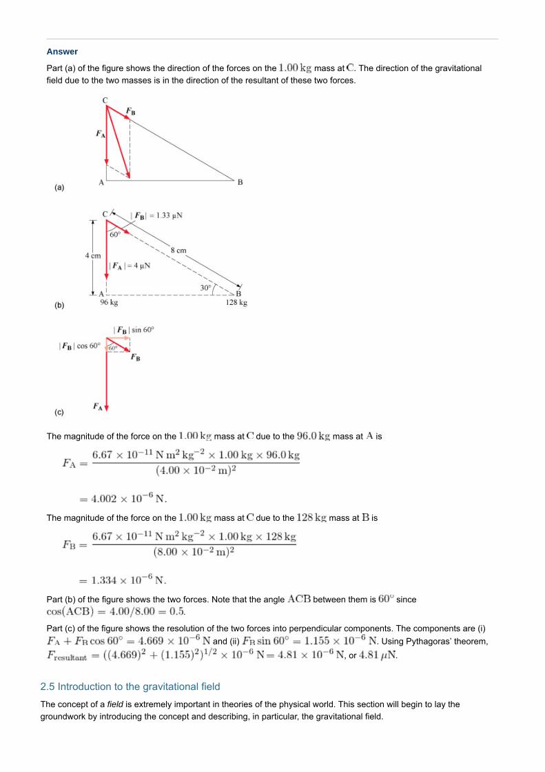
Answer

Part (a) of the figure shows the direction of the forces on the mass at . The direction of the gravitational

field due to the two masses is in the direction of the resultant of these two forces.

The magnitude of the force on the mass at due to the mass at is

The magnitude of the force on the mass at due to the mass at is

Part (b) of the figure shows the two forces. Note that the angle between them is since

.

Part (c) of the figure shows the resolution of the two forces into perpendicular components. The components are (i)

and (ii) . Using Pythagoras’ theorem,

, or .

2.5 Introduction to the gravitational field

The concept of a field is extremely important in theories of the physical world. This section will begin to lay the

groundwork by introducing the concept and describing, in particular, the gravitational field.

Example 2

A small body with mass is placed at a point designated as the origin as shown in the figure.

(a) Evaluate the magnitude and direction of the gravitational force on a point mass placed at the

point which is away from the origin and described by the position vector .

Answer

The gravitational force on the mass at due to the mass at the origin is given by Equation 6 (note that it is

proportional to :

(b) Using the result of part (a), evaluate the force (magnitude and direction) on a mass of placed at the

point .

Answer

As we noted, the force is proportional to , so when we double from to , with all of the other

values remaining unchanged, the force is also doubled, to ).

The important point to note about the case treated in Example 2 is that, once you have calculated the force on the

mass at , you do not need to use the value of to work out the force on a mass of at . This is a

very important conclusion, because it means that, given the force on a known mass at a particular point, we can calculate

the gravitational force on any mass placed at that point. Quite simply, the gravitational force is proportional to the mass

on which it is acting. One way of thinking about this situation is to imagine some vector, , associated with the point ,

that determines the gravitational force that would act on any mass placed at that point. This vector is called the

gravitational field at . A similar vector may be defined at every point in space, by dividing the gravitational force that

would act on an object of mass at any particular point by the value of . In this way, the gravitational field can be

defined at every point in space, even where there is no mass to experience a gravitational force. More precisely:

The gravitational field is a vector quantity, defined at all points in space. Its value at any particular point is given by the

gravitational force per unit ‘test’ mass at that point.

By a ‘test’ mass we mean a mass that experiences the effect of the gravitational field, but we specifically exclude the

possibility that the test mass will cause those masses that are responsible for creating the field to change their positions

and thereby change the gravitational field that is being investigated.

Because it is so important in physics, we will now spend some time on the field concept in general.

2.6 Vector and scalar fields

The concept of a field is a very important and much-used idea in physicists’ toolkits. Put into more precise language:

A field is a physical quantity to which a definite value can be ascribed at every point throughout some region of space.

In the case of a gravitational field, the quantity is the gravitational force per unit test mass. Because force is a vector

quantity, a gravitational field is represented by a vector at every point, and we therefore call it a vector field. However,

the general definition of a field simply refers to ‘a physical quantity’, and that quantity need not necessarily be a vector. A

scalar quantity might occur as a field too — only in that case it will be a scalar field. You may not have thought of it in

quite these terms before, but if you watch the TV weather forecasts you are in fact already quite familiar with examples of

both scalar and vector fields. Figure 9 shows two representations of temperature and pressure fields.

Figure 9 The temperature and pressure fields observed across

the British Isles one day in January 1981.

The temperature and pressure clearly fulfil the requirements of the definition in that they do have a value at every point in

the region considered (the British Isles). It would be impractical to measure them at every point, but one could certainly

obtain values for them at any point one cared to choose within the region. In one view of Figure 9, the temperature and

pressure values were measured at regularly spaced intervals, and written out as a grid. The second view shows another

representation of the fields, this time with ‘isotherms’ (lines connecting all points of equal temperature) and ‘isobars’ (lines

of equal pressure). This representation is much more graphic, and easier to interpret. Figure 9 shows examples of scalar

fields: temperature and atmospheric pressure are scalar quantities that are fully specified by a number and a unit. Wind

velocity, on the other hand, is a vector, and the wind velocity field is therefore a vector field: a direction as well as a

magnitude has to be assigned to every point in the field. The representation of the vector field is a little more difficult: in

Figure 10 it has been achieved using arrows.

Figure 10 The wind velocity field for the same day.

2.7 Defining the gravitational field

We have already defined the gravitational field at a point as the force per unit mass at that point, and noted that it must

be a vector. This can be expressed more formally by defining the point by its position vector , and writing:

Note that this is a vector equation, so it contains information about both the magnitude and the direction of the

gravitational field. Thus:

and

All of this information can be neatly contained in the following general definition:

Gravitational field

Equation 7 contains a very important kind of notational shorthand. The notation ) means the gravitational field at the

point whose position vector is . It does not mean multiplied by . The reason for using notation like this is because, in

general, the gravitational field will vary with position. If we move to a different point with a different position vector, the

gravitational field will usually have a different value. Another way of describing this type of situation is to say that is a

function of .

The position vector notation is an extremely useful one in the context of fields. Figure 11a is essentially the same as that

in Example 2, and shows again how the point referred to there may be defined in terms of a position vector. To explain

how to get somewhere, the first thing to do is to define the starting place. The starting place is effectively already defined

by putting mass at the origin . The gravitational field at is due to the presence of , so it is entirely reasonable

that the site of should be chosen to define our starting place. Once we have chosen the fixed point , however, there

are several ways in which we could explain how to get to point . One way is to use a position vector. An alternative

approach would be to make the origin of a set of coordinates (Figure 11b) and describe as the point ( , , . In that

case, the gravitational field would be written as

In the rest of this section, we shall continue to use the position vector notation, but you should appreciate the equivalence

of Equation 7 and Equation 8.

Figure 11 Alternative, but equivalent, ways of defining the

position of point : (a) by the position vector and (b) by its

coordinates Note that .

Let us now derive what is the SI unit for the magnitude of a gravitational field. From Equation 7, the unit for the magnitude

of ) must be that of force divided by that of mass, that is, . This is equivalent to the unit of acceleration

(remember Newton’s second law of motion) that is, . The magnitude of the gravitational field is the magnitude of

the local acceleration due to gravity. But remember that the gravitational field varies from place to place and it is a vector.

(7)

(8)

The frequently quoted is the magnitude at the surface of the Earth only. Even for places with the same

magnitude for , the direction will be different (see Figure 12).

Figure 12 The direction of the gravitational field at the surface of

a supposedly spherical Earth. The magnitudes are assumed to be

the same, but note the different directions (toward the centre of the

Earth in each case).

Let us now apply the general definition of a gravitational field, contained in Equation 7, to a particular situation, the one

first described and illustrated in Example 2. What is the gravitational field at the point ? Well, in the example you saw

that the gravitational force on the mass at the point due to the mass at the origin has magnitude

and is pointing along the direction of . The shorthand way of writing this is:

since is, as you will remember, a unit vector in the -direction. Equation 7 then gives

Thus, the gravitational field at , due to the mass , is of magnitude and is in the direction of

.

In Example 2 and subsequently, the notation has allowed us to make a distinction between a mass that we wish to

consider to be the source of a gravitational field (labelled by an upper case or capital letter ) and a mass that we wish

to consider to be ‘feeling the effects of’ the gravitational field (given the symbol lower case ). You should be aware that,

although this distinction can sometimes be useful, it is actually quite artificial. Two masses and , separated by a

distance , will each exert an attractive force on the other, the magnitude of which, in either case, is given by

2.8 The force on a particle in a gravitational field

The gravitational field is defined as the gravitational force per unit mass at any point in space. This leads to the following

very simple expression for the gravitational force experienced by a particle of any mass, , at any point in a known

gravitational field :

So, to find the force on a mass at position , one simply multiplies the value of the gravitational field at position by

the mass in question. Notice that the direction of the force is completely accounted for in this equation by the direction of

the gravitational field, since is a positive quantity.

Exercise 5

Consider a mass of placed in a region where there is a gravitational field of in the -direction.

What would be the force on this mass?

Answer

Because the field is in the -direction, so is the force and we can use the component form of Equation 9:

2.9 The gravitational field due to a point particle

We are now in a position to work out the gravitational field at an arbitrary displacement from a point mass .

Suppose we were to use a ‘test’ particle of mass to measure the gravitational force due to the fixed mass . Then,

from Newton’s law of universal gravitation,

But, according to Equation 9,

Comparing the two expressions for , we see that the gravitational field due to a point mass at the origin is:

This tells us that the magnitude of the gravitational field at displacement from a point mass is

Note also that, although represents a magnitude, and must therefore be a positive quantity, the gravitational force is

always attractive, so the field will point in the negative -direction. However, you should be very careful in interpreting

this. Remember that Equation 10 describes the gravitational field at a position measured from the mass that is the

source of the gravitational field. It is only because we chose, for convenience, to measure position vectors from the

position of mass that is in the negative -direction. Had we chosen to measure positions from some other

origin, then would not have been in the negative -direction. It is very important to remember that means the

gravitational field vector at position with respect to some specified origin. In general, the direction of is not the

direction of (or ).

Remember that, when the field is produced by a spherically symmetric body, then the gravitational effect outside the body

is the same as if all the mass of the body were concentrated at a point at the centre of the sphere. So Equation 10 will

also describe the gravitational field due to the Earth for points at, and above, the Earth’s surface:

This may be visualised by drawing the vector at various representative points above the surface.

(9)

(10)

(11)

Figure 13 The Earth’s gravitational field vector at various

points above the Earth’s surface.

Show transcriptDownloadAudio 2 The Earth’s

gravitational field

When solving mechanics problems, we can generally ignore the vector field properties of the gravitational field if we are

dealing with problems on the laboratory or similar local scale. In this case, we can regard as a vector that has the

same magnitude and direction throughout the entire region of interest. Such a vector field is called a uniform field. A

uniform field can be represented by the same vector at every point, as illustrated in Figure 14.

Figure 14 A uniform field is constant in both magnitude and

direction.

3 A first look at charge

In earlier Units, you discovered the effects of forces on bodies, effects summarised in Newton’s three laws of motion. In

the previous section of this Unit you have learned about one of the fundamental forces of nature, namely the gravitational

force, which not only holds the Earth in its orbit around the Sun but also holds us fairly firmly on the Earth’s surface. In

this section, we shall look at another force, the electrostatic force. This is the force responsible for binding atomic

electrons to nuclei and for holding atoms together to form microscopic molecules and macroscopic solids. In spite of its

name, the electrostatic force exists between moving charges as well as stationary ones. In later sections you will discover

that there are forces that only apply to moving charges, which is the reason for using the term electrostatic in this case.

3.1 Some simple electrostatic phenomena

Although electrostatic forces are, in general, not as apparent in everyday life as gravitational forces, it is quite easy to

perform elementary electrostatic experiments and you should try a couple now.

Activity 2: Moving objects with static electricity

Experiment 1

You will need: a plastic comb; a water tap; a head of hair (yours or a friend!).

Method: Turn on the tap, and adjust the flow until you have a steady stream of water that is or millimetres in

diameter. Brush your hair several times with the comb, then slowly bring the teeth of the comb towards the water, a

few centimetres below the tap. You should see the stream of water bend towards the comb.

Does it make a difference how close to the stream you bring the comb? What if you brush your hair more vigorously

or for longer, how does that alter the observed effect? Does the size of the stream of water make a difference?

Experiment 2

You will need: an empty drinks can; a balloon; a woollen article of clothing such as a jumper.

Method: Place the can on its side on a smooth surface. Rub the balloon on a woollen jumper vigorously for several

seconds. Now hold the balloon close to the can without touching it. You should see the can roll towards the balloon,

as you bring the balloon close to it.

Does it make a difference how close to the can you bring the balloon? What if you rub the jumper more vigorously

with the balloon or for longer, how does that alter the movement of the can? Does it make a difference if you use a

can that is full of liquid?

We shall return to consider an explanation for your observations in the next subsection. In fact, electrostatic phenomena

are the basis of some other well-known effects too. Clingfilm sticks to itself and to containers because of electrostatic

forces (Figure 15). You will almost certainly have seen a balloon stuck to the ceiling of a dry room after it has been

rubbed on woollen clothing or something similar. In this situation, the electrostatic attraction between the balloon and

ceiling is sufficiently large that it exceeds the gravitational force on the balloon and so the balloon does not fall. A similar

experiment involves rubbing a piece of plastic, such as a ruler, on a woollen cloth. The ruler may then be used to lift small

pieces of tissue paper, rather as a magnet lifts a steel nail. However, unlike the magnet, the ruler cannot continue to

provide the lifting force indefinitely, and eventually the tissue will drop from the ruler. Another example of the action of

electrostatic forces can be seen when brushing your hair in front of a mirror. If your hair is dry and you brush vigorously,

you will notice that the hair is attracted towards the brush. The same ‘static cling’ effect causes synthetic clothing to stick

to you (and, incidentally, to crackle) in dry weather.

Figure 15 It is electrostatic forces that cause clingfilm to cling.

In all these instances, the electrostatic force produced is comparatively large. Later in this Unit, you will discover why

electrostatic forces of such strength are not often observed in everyday life. But before we can study the force itself, we

must find out under what circumstances bodies like balloons, rulers and hair experience electrostatic forces. Clearly,

bodies do not always experience these electrostatic forces — your hair doesn’t always stand on end! Something must

have happened in each case during the rubbing process to make the bodies experience an electrostatic force. This fact is

conveniently expressed in the statement that bodies that experience electrostatic forces are charged with electricity. In

this section, you will discover some of the properties of this electric charge and consider how electrostatic charging

takes place.

3.2 Electric charge

During the 18th century, a number of distinguished and ingenious scientists carried out simple experiments, similar to

those described in the previous section, which clarified the nature of electric charge. These experiments culminated in

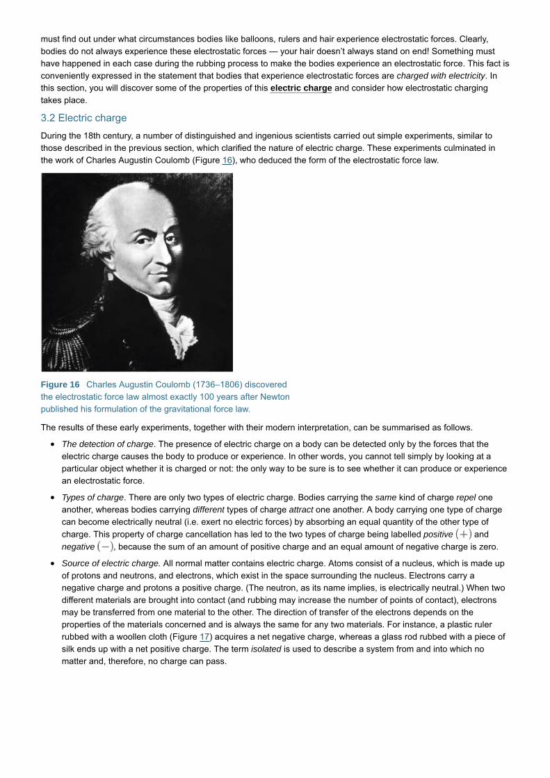
the work of Charles Augustin Coulomb (Figure 16), who deduced the form of the electrostatic force law.

Figure 16 Charles Augustin Coulomb (1736–1806) discovered

the electrostatic force law almost exactly 100 years after Newton

published his formulation of the gravitational force law.

The results of these early experiments, together with their modern interpretation, can be summarised as follows.

The detection of charge. The presence of electric charge on a body can be detected only by the forces that the

electric charge causes the body to produce or experience. In other words, you cannot tell simply by looking at a

particular object whether it is charged or not: the only way to be sure is to see whether it can produce or experience

an electrostatic force.

Types of charge. There are only two types of electric charge. Bodies carrying the same kind of charge repel one

another, whereas bodies carrying different types of charge attract one another. A body carrying one type of charge

can become electrically neutral (i.e. exert no electric forces) by absorbing an equal quantity of the other type of

charge. This property of charge cancellation has led to the two types of charge being labelled positive and

negative , because the sum of an amount of positive charge and an equal amount of negative charge is zero.

Source of electric charge. All normal matter contains electric charge. Atoms consist of a nucleus, which is made up

of protons and neutrons, and electrons, which exist in the space surrounding the nucleus. Electrons carry a

negative charge and protons a positive charge. (The neutron, as its name implies, is electrically neutral.) When two

different materials are brought into contact (and rubbing may increase the number of points of contact), electrons

may be transferred from one material to the other. The direction of transfer of the electrons depends on the

properties of the materials concerned and is always the same for any two materials. For instance, a plastic ruler

rubbed with a woollen cloth (Figure 17) acquires a net negative charge, whereas a glass rod rubbed with a piece of

silk ends up with a net positive charge. The term isolated is used to describe a system from and into which no

matter and, therefore, no charge can pass.

Figure 17 Charging by rubbing. When a plastic ruler is rubbed

with a woollen cloth, electrons flow from the wool to the plastic.

This process will leave an excess of electrons on the plastic so

that it carries a net negative charge whereas the wool, with a

deficit of electrons, carries a positive charge of equal magnitude.

Conservation of charge. In the rubbing process illustrated in Figure 17, no charge has been created: existing

charges have simply been redistributed between the wool and the plastic. In fact, the total amount of charge in any

isolated system is always constant. In other words:

In an isolated system, the total electric charge is always conserved.

The law of conservation of charge takes its place alongside the laws of conservation of linear momentum, angular

momentum and energy as one of the fundamental laws of physics. The conservation of charge does not imply that

charges can never be created or destroyed, but it does imply that for any positive charge created, an equal amount

of negative charge must also appear. An example illustrating the law of conservation of charge is shown in

Figure 18.

View larger imageFigure 18 Examples of charge conservation in

high-energy physics. (a) A famous bubble chamber photograph

that confirmed the existence of the -particle. (b)

Interpretation of the tracks: the various particles are identified by

letters. The tracks of positive and negative particles curve in

opposite directions (the reason for this will become clear once

you have studied Unit 11). Particles with superscript 0 are

neutral and do not leave tracks, so they are identified by their

decay products. Notice particularly the decay of the neutral

into a proton (p) and a negatively charged pion ( : total

charge is conserved because equal amounts of positive and

negative charge have been created.

Conduction of charge. Because bodies carrying unlike charges attract one another, any body that has a deficit of

electrons (i.e. any body that carries a net positive charge) will not only attract negatively charged macroscopic

bodies in the vicinity, but will also attract any electrons that are close by. If these electrons are free to move, they

will flow towards the positively charged body and neutralise it. It is this process of charge redistribution that prevents

us detecting the electric charge on a hand-held rod of copper when it is rubbed. When copper is rubbed, it does

acquire a charge. However, copper has the property that electric charge can flow easily through it and so the

imbalance of charge in the rubbed region can be made good by electrons flowing through the rod to or from the

hand holding the end of the rod. Materials that allow electric charge to flow through them are called conductors

and those that do not are called insulators. Glass and plastic are examples of insulators, whereas metals and

seawater are conductors.

Certain materials behave like perfect insulators for small electrostatic forces only. When the electrostatic force increases,

there comes a point when electrons can be detached from the atoms of the material and these electrons can then move

a short distance. This movement of electrons is equivalent to a charge flow through the material. The material is said to

have suffered electrical breakdown and become conducting. This behaviour can theoretically occur in all insulators. In

most solid insulators, however, the force required to produce breakdown is so large that the effect can often be

neglected. In gases, on the other hand, the occurrence of electrical breakdown is quite common. Have you ever noticed

sparks when you undress in a darkened room? This is the result of the electrical breakdown of air. Clothes made from

synthetic fibres can become charged through the rubbing involved in everyday movement. When you undress, you

separate oppositely charged regions. When breakdown occurs, these regions can exchange charge through the air that

separates them. Some of the air molecules become excited by the charge flow and then lose this surplus energy by

emitting visible radiation. This causes the observed spark.

Exercise 6

Bearing in mind the discussion above, suggest an explanation for the observations you made in the two experiments

you carried out earlier.

Answer

Hair or wool and plastic (in the comb) or rubber (in the balloon) are good at exchanging charge when they are rubbed

together. The comb and balloon each acquire a net excess of negative charge as they remove electrons from your

hair or the woollen jumper, which become positively charged as a result of losing electrons.

When the negatively charged comb is brought close to the stream of water (or the negatively charged balloon is

brought close to the empty can), the water (or can) is attracted to the charged comb (or balloon). An explanation is as

follows. In the case of the stream of water, the water molecules are said to be polarised — they carry both positive

and negative charge. The negatively charged comb orients the nearby water molecules so that the positive charges

are closest to the comb, which then attracts the stream of water towards it. In the case of the can, the metal contains

free electrons that are repelled by the negatively charged balloon, resulting in a net positive charge in the metal

nearest to the balloon. As a result the balloon attracts the can, which rolls towards it.

The closer you bring the comb to the water, or the balloon to the can, the larger is the movement seen. This suggests

that the electrostatic force becomes stronger as distance decreases. Combing or rubbing the hair or jumper more

vigorously results in an increased movement of the water or can. This suggests that a greater net negative charge has

been acquired by the comb or balloon as a result. Finally, using a larger stream of water or a heavier can results in

less (or no) movement of the stream or the can. This suggests that the electrostatic force in this experiment is rather

weak and can be overcome by gravity when the mass of the water or can is increased.

In the next section you will see in more detail the question of charge distribution and the way in which spontaneous or

induced redistribution of charge takes place. Before moving on to these topics, make sure that you can list the main

properties of electric charge. The box below provides a checklist of important points.

The main properties of electric charge

The presence of a net electric charge on a body can be detected only via electrostatic forces.

There are only two types of charge: these are labelled as positive and negative. Like charges repel and unlike

charges attract one another.

Charge is a conserved quantity.

All normal matter contains charge, and in certain circumstances this can be transferred from one body to

another.

Charge can flow easily through certain substances; such materials are called conductors. Other substances,

through which charge cannot easily flow, are called insulators.

Exercise 7

Two identical brushes are charged by vigorously brushing a dry moulting dog. (a) Will the hairs that fall out attract or

repel one another? (b) Will the hairs be attracted to the brush or repelled from it? (c) Will the two brushes attract or

repel each other?

Answer

In the brushing process, charge will be transferred from the hairs to the brushes. This will leave the hairs carrying one

type of charge and the brushes with the opposite charge.

(a) The hairs carry like charges and so repel one another.

(b) The hairs carry the opposite type of charge to the brush and will be attracted to the brush.

(c) The brushes carry like charges and so repel each other.

3.3 The distribution of electric charge

You may now be wondering why the electrostatic force is not more apparent in everyday life. Matter has two basic

properties that cause it to exert forces: one of these properties is mass, which produces gravitational forces, and the

other is charge, which produces electrostatic forces. Yet, although we are aware of the gravitational force as soon as we

fall out of bed in the morning, we usually have to perform an experiment before we become conscious of the electrostatic

force. One of the reasons for this apparent paradox arises from the fact that there are two types of charge, positive and

negative, but only one type of mass. The attraction between two equally but oppositely charged objects, and the resulting

charge cancellation when they coalesce, produces a single electrically neutral body that does not exert a net electrostatic

force. This explains why most lumps of matter contain precisely equal amounts of positive and negative charge and are

therefore electrically neutral. However, because there is only one kind of mass, which always gives rise to an attractive

gravitational force, two objects coalescing will simply form a more massive body that will exert an even greater

gravitational force on other masses. As you will shortly see, the gravitational force is extraordinarily weak, but this is

compensated by the very large mass of bodies such as the Earth, that exert significant gravitational forces. Although

electrostatic forces are not often immediately apparent in nature, they can, under certain circumstances, produce very

dramatic effects. In the audio files below we talk about the conditions that give rise to hazardous manifestations of

electrostatic forces: lightning storms and the occasional explosion of oil tankers during cleaning.

Figure 19 Schematic diagram of the charge distribution in a

typical fully developed thundercloud. Note the thickness of the

cloud, and the temperature difference across it. Two separate

discharge processes are shown.

Figure 20 A lightning discharge. Although the visual effect is

dramatic, the amount of energy liberated in an average lightning

flash is modest about the equivalent of the energy liberated in

the explosion of a gallon of oil.

Show transcriptDownloadAudio 3 Lightning storms

Figure 21 Charging by rubbing takes place as liquids flow

through pipes. The charge separation between a pipe and its

contents can have disastrous results in an oil tanker because of

the highly explosive nature of oil vapour.

Show transcriptDownloadAudio 4 Oil tanker explosions

3.4 Charging by sharing and induction

Lightning and oil tanker explosions are striking illustrations of charge redistribution. Neither phenomenon is totally

understood, and work is still being done to clarify the mechanisms of charge separation. However, we shall now turn our

attention to a pair of well-understood methods by which charges may be redistributed. These methods were of great

importance historically, because in the early days of electrostatic experimentation there was no absolute measure of

quantity of charge. By using these two techniques, it was possible to give bodies identical charges in one case and

opposite charges of equal magnitude in the other. This allowed Coulomb to perform quantitative experiments on the

forces between two charged bodies without knowing the absolute charge on either body.

The first process we shall look at is charge sharing between two identical bodies, say two spheres and made of

some conducting material and mounted on insulating stands (Figure 22a). Sphere is charged, perhaps by rubbing it on

some cloth (remember this can only be done provided the metal is not touched by the hand). Sphere is then brought

up to touch the initially neutral sphere . Since the excess charges on repel one another and since they can flow

freely through the conducting material of the spheres, will immediately acquire a charge (Figure 22b). When the

spheres are separated again (Figure 22c), the charges will redistribute themselves uniformly, with the original charge

shared equally between the two spheres.

View larger imageFigure 22 Charge sharing between conducting

spheres. (a) Sphere is initially given a positive charge 2 , and

sphere is neutral. (b) The charge spreads over both spheres

when they are brought into contact. (c) When and are

separated, the charge left on each of them is half that originally

given to .

The second process by which charges may be redistributed is known as induction. This method has the advantage that

the original charge may be used to repeat the process again and again. The principle of the method is illustrated in

Figure 23. Two uncharged metal spheres on insulating supports are placed in contact with each other (Figure 23a). When

a negatively charged rod is brought close to sphere but without touching it, some of the electrons within are repelled

by the charges on the rod and flow to sphere , leaving a net positive charge on and a net negative charge on . The

resulting charge distribution is shown in Figure 23b. The excess positive charge on the sphere closer to the rod is called

the induced positive charge, and the excess negative charge on the other sphere is called the induced negative charge.

View larger imageFigure 23 Charging by induction. In this case,

both spheres are initially neutral (a) and it is a third body that is

charged by rubbing and brought close to them (b). When the

spheres are separated and the third body removed, the charge

left on one of the spheres is opposite in sign but equal in

magnitude to that left on the other.

Exercise 8

Give a description of the final stages of charging by induction as illustrated in Figure 23c, 23d and 23e.

Answer

Figure 23c: When the spheres are separated, the one closer to the rod carries an excess positive charge, which is

concentrated towards the rod. The other sphere is left with an excess negative charge, which is repelled towards the

right by the charge on the rod.

Figure 23d: When the rod is removed and the spheres are still sufficiently close to interact, the distribution of the

excess charge changes since unlike charges attract each other. The total excess charge on each of the spheres is

unaffected.

Figure 23e: When the spheres are a large distance apart, they carry equal and opposite charges distributed uniformly

over their surfaces.

4 Electrostatic forces and fields

So far, we have not considered the magnitude of an electrostatic force, only the circumstances under which such a force

exists and whether it is attractive or repulsive. In this section, the description of the electrostatic force will be put on a

quantitative footing, and the associated field will be introduced.

4.1 The electrostatic forces between two charges

4.1.1 Coulomb’s experiment

Coulomb became, in 1785, the first person to establish the dependence of the electrostatic force on the distance between

the charges. He considered the force between two very small charged bodies (i.e. bodies whose diameters were much

smaller than the distance between them). This size restriction allowed him to assume that all the charge on each of the

bodies was concentrated at a point. These very small charged bodies are often referred to as point charges. Their use

allowed Coulomb to neglect the problem of how charge is distributed throughout a body. In fact, once Coulomb had

established the magnitude of the force between point charges, it was a small step to extend the result to more complex

charge distributions, since any charge distribution can be thought of as composed of a large number of point charges.

The experimental situation investigated by Coulomb is shown schematically in Figure 24.

Figure 24 The essential details of the apparatus with which

Coulomb investigated the dependence of the electrostatic force on

the magnitude and separation of two ‘point charges’.

A point charge is separated from another point charge by a distance . Because he had no means of measuring

charge, Coulomb used small identical conducting spheres for the bodies so that he could successively halve the values

of and by sharing the charge with identical uncharged spheres, as illustrated earlier in Figure 22. Using a very

sensitive torsion balance (Figure 25) to measure the forces on the charges, Coulomb was able to show that the

magnitude, , of the electrostatic force acting on due to was:

inversely proportional to , when the magnitudes of and were fixed;

proportional to the magnitude of , when and were fixed;

proportional to the magnitude of , when and were fixed.

Thus, in mathematical symbols: , and . These three results can be combined to

give the single proportionality

(12)

Figure 25 Coulomb’s torsion balance. The force between

the two small charged spheres causes a torque to act on the

long horizontal beam. By twisting the wire at the suspension

point, an opposite and equal torque can be applied. With

zero net torque, the beam’s position remains unchanged.

The angle through which the suspension must be twisted to

achieve this result is proportional to the electrostatic force.

The whole apparatus is enclosed in a case because the

forces involved are small and draughts could easily

introduce appreciable errors.

4.1.2 The strength of the electrostatic interaction

To turn this proportionality into an equation, all that is necessary is to introduce a proportionality constant. But to give a

value to that constant, we need to know the unit in which and are measured. The SI unit of charge is called, very

appropriately, the coulomb (given the symbol C). The proper definition of the coulomb depends on the magnetic force, in

a way that will be discussed in Unit 11, but, to give you some idea of the size of the unit of charge, it is worth noting that

the total charge delivered by a typical lightning bolt is, very roughly, .

If the charges and are located in a vacuum, the proportionality constant for the electrostatic force law is normally

written in the form . The magnitude of the electrostatic force in a vacuum is thus

The quantity ( is the Greek letter epsilon) is known as the permittivity of free space. Experiments show that the

value of is .

(13)

Exercise 9

Jot down an argument to convince another student that the unit of the proportionality constant is .

Answer

Equation 13 can be rearranged to give

The unit of is therefore that of , which is .

You should notice the similarity between Equation 13 and the equation for the gravitational force between two masses

(Equation 2) that you met earlier. In both gravitational and electrostatic interactions, the force is inversely proportional to

the square of the distance between the particles. However, the two interactions have rather different strengths, as you

can discover by answering the following question.

Exercise 10

(a) What is the magnitude of the force between two charges, each of , separated by in free space? (You

may take the value for to be .)

Answer

Coulomb’s law states that the magnitude of the electrostatic force in a vacuum is given by

(b) On what mass of iron would the gravitational force at the Earth’s surface have this magnitude?

Answer

The magnitude of the gravitational force on a mass at the surface of the Earth is given by . The

mass of iron on which the gravitational force is of magnitude is therefore

This is almost million tonnes!

The answer suggests one of two things: either that the electrostatic force is immensely strong, or that the coulomb is a

very large unit of charge. In fact, there is some truth in both of these possibilities. The coulomb is, in practical terms, a

very large amount of charge. The reason for choosing such a large standard unit of charge will become clear when you

meet the magnetic force law in Unit 11. In this Unit and in Unit 9, however, you will also be concerned with the charge

carried by electrons. The electron charge (denoted by is very small indeed:

Note the minus sign: the electron carries a negative charge. Protons are the positively charged constituents of the nuclei

of atoms; each has charge .

From a qualitative point of view, we would say that the electrostatic force is very much stronger than the gravitational

force. However, it is not possible to make any fundamental quantitative comparison of the two forces because our units of

charge and mass (the coulomb and the kilogram) are not fundamental in any way: they are to a large extent arbitrary.

However, the following example allows you to compare the magnitudes of the electric and gravitational forces on an

atomic scale.

Example 3

The hydrogen atom may be modelled as an electron orbiting a proton in a circular orbit of radius .

Treating the proton and the electron as point charges, estimate the ratio of the electrostatic force to the gravitational

force between the two particles. You may take the masses of the proton and the electron to be and

, respectively. The constants are: and

.

Answer

The electrostatic force has magnitude

and the gravitational force has magnitude

The ratio of these is

To emphasise the overwhelming importance of the orders of magnitude, we make the following approximations:

Inserting these values gives

A more exact calculation gives a value of for the ratio of the strength of the electrostatic force to the

gravitational force in this case.

The value of was first measured accurately by Robert A. Millikan. His method will be explained later in this Unit. The

importance of the charge on an electron is that it is generally believed to be the smallest amount of charge that can have

an independent existence and be transferred from one body to another. In a rubbing experiment, you might transfer about

electrons (i.e. a charge of about ) to the object being rubbed. This may seem like a huge number of

electrons. It is, however, only a tiny fraction, about in , of the total number of electrons in the object. Because the

electron charge is so small, in macroscopic electrostatics we can assume electric charge to be infinitely divisible and

continuous and we can ignore its ‘graininess’. We may, for example, imagine that a negatively charged body has the

charge spread continuously over it, rather than worry about the finite number of separate electrons acting as point

charges. We do exactly the same thing in dealing with the mass of an ordinary object: we imagine it to be infinitely

divisible, although the atomic nature or ‘graininess’ of all matter implies that it is not really so.

4.2 Coulomb’s law

Exercise 11

The figure shows three charges arranged in a straight line. Charges and are held fixed in position.

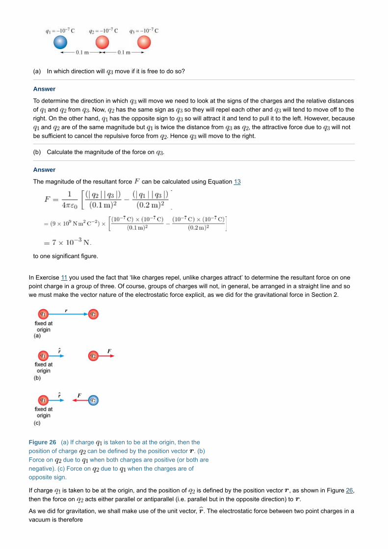
(a) In which direction will move if it is free to do so?

Answer

To determine the direction in which will move we need to look at the signs of the charges and the relative distances

of and from . Now, has the same sign as so they will repel each other and will tend to move off to the

right. On the other hand, has the opposite sign to so will attract it and tend to pull it to the left. However, because

and are of the same magnitude but is twice the distance from as , the attractive force due to will not

be sufficient to cancel the repulsive force from . Hence will move to the right.

(b) Calculate the magnitude of the force on .

Answer

The magnitude of the resultant force can be calculated using Equation 13

to one significant figure.

In Exercise 11 you used the fact that ‘like charges repel, unlike charges attract’ to determine the resultant force on one

point charge in a group of three. Of course, groups of charges will not, in general, be arranged in a straight line and so

we must make the vector nature of the electrostatic force explicit, as we did for the gravitational force in Section 2.

Figure 26 (a) If charge is taken to be at the origin, then the

position of charge can be defined by the position vector . (b)

Force on due to when both charges are positive (or both are

negative). (c) Force on due to when the charges are of

opposite sign.

If charge is taken to be at the origin, and the position of is defined by the position vector , as shown in Figure 26,

then the force on acts either parallel or antiparallel (i.e. parallel but in the opposite direction) to .

As we did for gravitation, we shall make use of the unit vector, . The electrostatic force between two point charges in a

vacuum is therefore

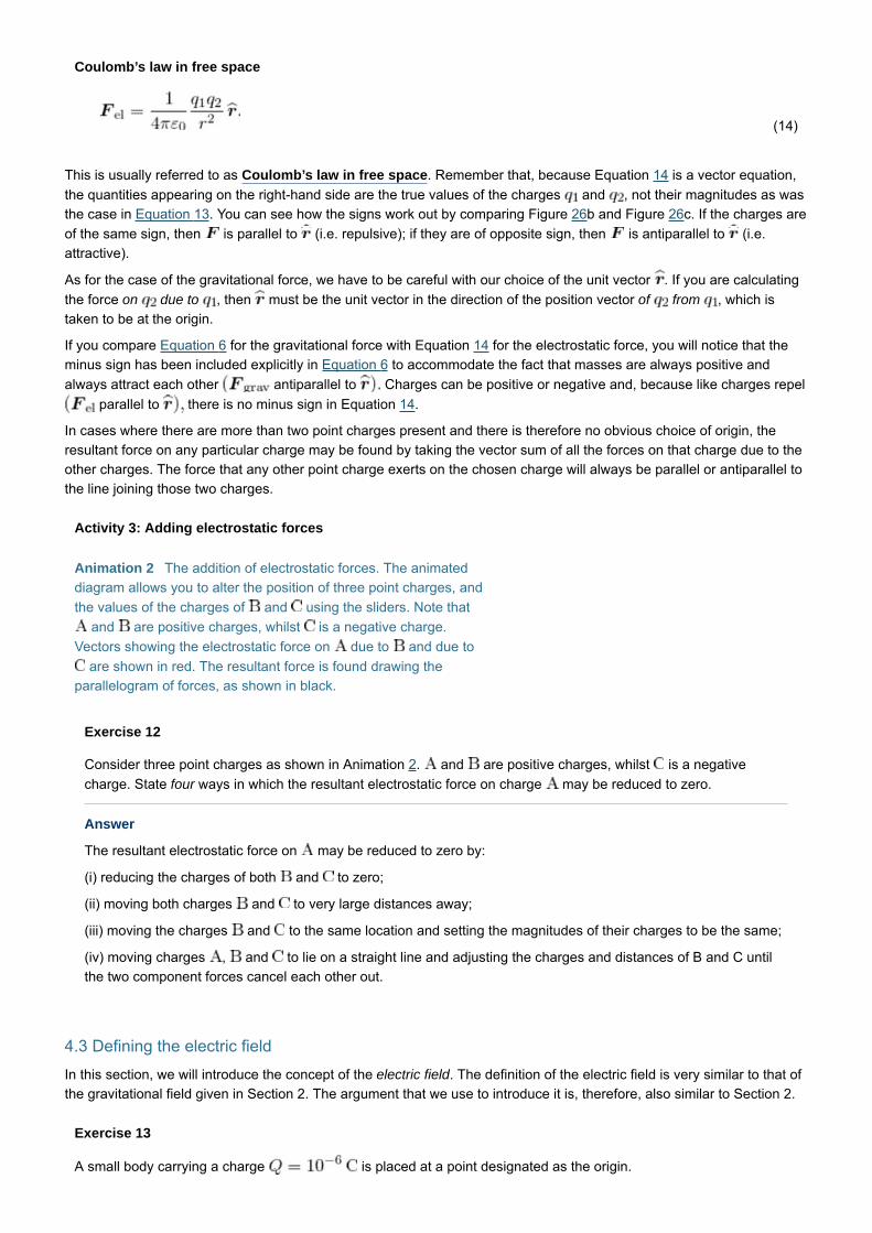
Coulomb’s law in free space

This is usually referred to as Coulomb’s law in free space. Remember that, because Equation 14 is a vector equation,

the quantities appearing on the right-hand side are the true values of the charges and , not their magnitudes as was

the case in Equation 13. You can see how the signs work out by comparing Figure 26b and Figure 26c. If the charges are

of the same sign, then is parallel to (i.e. repulsive); if they are of opposite sign, then is antiparallel to (i.e.

attractive).

As for the case of the gravitational force, we have to be careful with our choice of the unit vector . If you are calculating

the force on due to , then must be the unit vector in the direction of the position vector of from , which is

taken to be at the origin.

If you compare Equation 6 for the gravitational force with Equation 14 for the electrostatic force, you will notice that the

minus sign has been included explicitly in Equation 6 to accommodate the fact that masses are always positive and

always attract each other antiparallel to Charges can be positive or negative and, because like charges repel

parallel to there is no minus sign in Equation 14.

In cases where there are more than two point charges present and there is therefore no obvious choice of origin, the

resultant force on any particular charge may be found by taking the vector sum of all the forces on that charge due to the

other charges. The force that any other point charge exerts on the chosen charge will always be parallel or antiparallel to

the line joining those two charges.

Activity 3: Adding electrostatic forces

Animation 2 The addition of electrostatic forces. The animated

diagram allows you to alter the position of three point charges, and

the values of the charges of and using the sliders. Note that

and are positive charges, whilst is a negative charge.

Vectors showing the electrostatic force on due to and due to

are shown in red. The resultant force is found drawing the

parallelogram of forces, as shown in black.

Exercise 12

Consider three point charges as shown in Animation 2. and are positive charges, whilst is a negative

charge. State four ways in which the resultant electrostatic force on charge may be reduced to zero.

Answer

The resultant electrostatic force on may be reduced to zero by:

(i) reducing the charges of both and to zero;

(ii) moving both charges and to very large distances away;

(iii) moving the charges and to the same location and setting the magnitudes of their charges to be the same;

(iv) moving charges , and to lie on a straight line and adjusting the charges and distances of B and C until

the two component forces cancel each other out.

4.3 Defining the electric field

In this section, we will introduce the concept of the electric field. The definition of the electric field is very similar to that of

the gravitational field given in Section 2. The argument that we use to introduce it is, therefore, also similar to Section 2.

Exercise 13

A small body carrying a charge is placed at a point designated as the origin.

(14)

(a) Evaluate the magnitude and direction of the electrostatic force on a point charge placed at the

point , which is away from the origin and described by the position vector .

Answer

Because the two charges have the same sign, the force will be repulsive, and the force on the charge at point will

be in the direction of the position vector . The magnitude of the force is

(b) Using the result of part (a), evaluate the force (magnitude and direction) on a charge of placed at

the point .

Answer

From Coulomb’s law, the force on a charge is proportional to the charge . In (a), we showed that

. Thus if is doubled in magnitude, the force will be doubled, but it will act in the same direction.

Hence, and acts in the direction of the position vector . Notice that there was no need to

refer to in finding this force; knowledge of the force on the charge was sufficient.

From the example treated in Exercise 13 it is clear that the electrostatic force experienced by a charge at a certain

point is proportional to the charge . Thus, we may define the electric field at that point as the electrostatic force that

would act on a charge placed at that point, divided by the value of the charge. In this way, the electric field can be defined

at any point in space, even though there may be no charge at that point to experience an electrostatic force. More

precisely:

The electric field is a vector quantity defined at all points in space. Its value at any particular point is given by the

electrostatic force per unit positive test charge at that point.

This can be expressed mathematically by defining the point by its position vector , and writing:

This is a vector equation, so it contains information about both the magnitude and the direction of the electric field. Thus:

and

All of this information can be expressed in the following general definition:

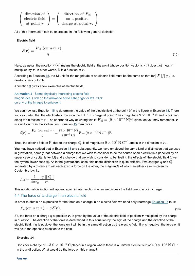
Electric field

Here, as usual, the notation means the electric field at the point whose position vector is : it does not mean

multiplied by . In other words, is a function of .

According to Equation 15, the SI unit for the magnitude of an electric field must be the same as that for , i.e.

newtons per coulomb.

Animation 3 gives a few examples of electric fields.

Animation 3 Some physically interesting electric field

magnitudes. Click on the arrows to scroll either right or left. Click

on any of the images to enlarge it.

We can now use Equation 15 to determine the value of the electric field at the point in the figure in Exercise 13. There

you calculated that the electrostatic force on the charge at point has magnitude and is pointing

along the direction of . The shorthand way of writing this is , since, as you may remember,

is a unit vector in the -direction. Equation 15 then gives

Thus, the electric field at , due to the charge , is of magnitude and is in the direction of .

You may have noticed that in Exercise 13 and subsequently, we have employed the same kind of distinction that we used

in gravitation, namely that between a charge that we wish to consider to be the source of an electric field (labelled by an

upper case or capital letter ) and a charge that we wish to consider to be ‘feeling the effects of’ the electric field (given

the symbol lower case ). As in the gravitational case, this useful distinction is quite artificial. Two charges and

separated by a distance will each exert a force on the other, the magnitude of which, in either case, is given by

Coulomb’s law, i.e.

This notational distinction will appear again in later sections when we discuss the field due to a point charge.

4.4 The force on a charge in an electric field

In order to obtain an expression for the force on a charge in an electric field we need only rearrange Equation 15 thus:

So, the force on a charge at position , is given by the value of the electric field at position multiplied by the charge

in question. The direction of the force is determined in this equation by the sign of the charge and the direction of the

electric field. If is positive, the force on it will be in the same direction as the electric field. If is negative, the force on it

will be in the opposite direction to the field.

Exercise 14

Consider a charge of placed in a region where there is a uniform electric field of

in the -direction. What would be the force on this charge?

Answer

(15)

(16)

Since the field is in the -direction, we can use the component form of Equation 16: , i.e.

. The minus sign shows that the force acts in the

opposite direction to the field.

A longer calculation, including both electric forces and equations of motion from earlier Units, is presented in the

problem-solving format in the following example.

Example 4

Electrons are emitted into a vacuum from a hot wire. They have negligible initial speed, and are then accelerated by a

uniform electric field of magnitude . What speed will the electrons have reached by the time they

have travelled from the wire?

To view the solution, click on Video 1 below. Full-screen display is recommended.

DownloadVideo 1 Solution to Example 4

4.5 The electric field due to a point charge

As an application of the general definition of the electric field, we can now formulate an expression for the electric field

at an arbitrary displacement from a point charge . Suppose we have a fixed point charge . A test charge at

would experience an electrostatic force due to given by Coulomb’s law:

But, according to Equation 16

Comparing the two expressions for we see that the electric field due to a point charge is

Equation 17 tells us two things. First, it tells us that the magnitude of the electric field at displacement from a charge

is

Note the modulus sign around the charge in Equation 18: this ensures that the magnitude of the electric field will

always be positive even if the source charge is negative. Note also that, although represents a magnitude, and is

therefore not emboldened, is still a position vector and therefore is emboldened. Secondly, Equation 17 shows that the

electric field is in the -direction if the charge is positive and in the -direction if is negative. Remember,

however, that is in the or -direction only because we chose to measure position vectors from the position of

charge . In general, the direction of is not the direction of or .

4.6 Addition of electric fields

Any charge will always be surrounded by an electric field. Now, suppose two or more charges are placed close together

so that their fields overlap. How can we work out their combined effect?

Well, a little algebra will show that adding fields is essentially the same process as adding forces. Figure 27 shows a

situation in which two source charges and interact with a third test charge placed at a point that has position

vector (in this case, with respect to some arbitrary origin that is not marked on the diagram).

(17)

(18)

Figure 27 (a) The charge at the point (defined by position

vector ) experiences forces and due to the presence of

the two charges and . (b) The resultant force on

at is equal to the vector sum of the individual forces acting on

it. This implies that the total electric field at the point , as tested

by a charge , is equal to the vector sum of the individual electric

fields due to each of the source charges separately.

Suppose that the fields produced individually by and are denoted, respectively, and . As experienced by the

test charge , the forces and due to these sources are ) and ), respectively. (This follows directly

from the definition of the electric field.) The resultant force, , on is obtained by adding the forces and

vectorially, as illustrated in Figure 27b. So

But the resultant electric field ) is defined by Equation 15 as the resultant electrostatic force per unit charge.

So in this case

Comparing equations, we must have

Thus, the resultant electric field is the vector sum of the individual electric fields produced by the two sources. In other

words, electric fields add vectorially just as forces do. Notice that, in this case, the electric field, ), is highly

unlikely to be in the direction of .

Exercise 15

A positive and a negative charge of equal magnitude are placed at a distance from each other on the -axis as

shown in the figure. Determine the direction of the electric field at point , which is equidistant from both charges.

Answer

The contributions to the field at due to the positive and negative charges are shown the figure. Their magnitudes

(19)

are the same, because the magnitudes of the two charges are the same, as are their distances from . The directions

are along the line joining to the charges and away from the positive charge but towards the negative charge. Thus,

the two contributions make equal angles above and below the positive -direction. The resultant field at is therefore

in the positive -direction.

Exercise 16

The figure shows two charges and , placed such that if is taken

to be at the origin of coordinates then is at the position , . Calculate the magnitude

and direction of the electric field at the point , which has coordinates , .

Answer

The directions of the two contributions to the total field at are shown on the figure. (Note that the magnitudes are

not necessarily drawn to scale — they are to be calculated.) These contributions can be calculated separately, and

then summed vectorially.

The field contribution at can be obtained either by using Equation 17 or by using Equation 18 together with the ’like

charges repel, unlike charges attract’ rule. By the latter method, the field at due to has components

and

The field at due to has components and

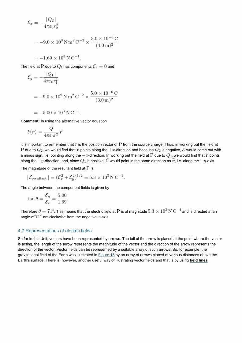
Comment: In using the alternative vector equation

it is important to remember that is the position vector of from the source charge. Thus, in working out the field at

due to , we would find that points along the -direction and because is negative, would come out with

a minus sign, i.e. pointing along the -direction. In working out the field at due to , we would find that points

along the -direction, and, since is positive, would point in the same direction as , i.e. along the -axis.

The magnitude of the resultant field at is

The angle between the component fields is given by

Therefore . This means that the electric field at is of magnitude and is directed at an

angle of anticlockwise from the negative -axis.

4.7 Representations of electric fields

So far in this Unit, vectors have been represented by arrows. The tail of the arrow is placed at the point where the vector

is acting, the length of the arrow represents the magnitude of the vector and the direction of the arrow represents the

direction of the vector. Vector fields can be represented by a suitable array of such arrows. So, for example, the

gravitational field of the Earth was illustrated in Figure 13 by an array of arrows placed at various distances above the

Earth’s surface. There is, however, another useful way of illustrating vector fields and that is by using field lines.

Figure 28 Michael Faraday (1791–1867).

Show transcriptDownloadAudio 5 Michael Faraday

Field lines were invented by Michael Faraday, for the purpose of illustrating electric fields. He imagined the space around

an array of point charges, for example, to be filled with directional field lines with the following two properties:

The tangent to the field line is parallel to the electric field at that point;

The lines are closer together where the field is strong and farther apart where it is weaker.

Thus the electric field round a point positive charge is represented by a set of radial lines pointing away from the charge

as in Figure 29a. If the charge is negative (Figure 29b) then the lines point towards the charge. Thus we have another

rule for electric field lines:

Field lines emerge from positive charges and disappear into negative charges.

View larger imageFigure 29 The electric field lines about (a) a

positive point charge and (b) a negative point charge. Here, we

have shown the field lines in three-dimensional perspective.

Usually, however, for the sake of clarity, they are shown only in

two dimensions, as in (c) positive charge and (d) negative

charge.

The number of field lines starting or ending on charges is proportional to the magnitude of the charge. In any one picture

you can choose the number of field lines per unit charge, but the chosen number must remain consistent within that

picture. Thus, the field around the two charges shown in Figure 30 has eight field lines emanating from the charge

and four ending on the charge. It is important to remember that field lines exist in all three dimensions, and the

spacings between them, and the number per unit charge, are accurately correct only in three dimensions. On paper, we

can generally show the field lines only in two dimensions, which involves taking some kind of cross-section through the

three-dimensional picture. Inevitably, this sometimes results in uneven spacings between the field lines.

Figure 30 The number of field lines starting or ending on a

charge is proportional to the magnitude of the charge. You should

remember that it is not always possible to get this accurately

correct in a two-dimensional representation of a three-dimensional

field.

A uniform field (one that has a constant magnitude and direction over the region of interest) is represented by a series of

equally spaced, parallel field lines. One way of creating a uniform electric field is by placing equal and opposite charges

on each of two large, closely spaced parallel conducting plates (Figure 31). Then the region between the plates contains

a uniform electric field.

Figure 31 A uniform electric field between two oppositely

charged, parallel plates.

There is one other important feature of field lines that you may have noticed: field lines never intersect. In other words,

they never cross each other.

But why do field lines not intersect?

Suppose for a moment this did occur (see Figure 32). At the intersection point , the field would have to be

simultaneously parallel to two lines that point in different directions. This is clearly a contradiction — the field has a

definite direction (not a choice of two!). The supposition that field lines may intersect cannot be true.

Figure 32 The situation if field lines were to intersect.

Exercise 17

Do charged particles always move along electric field lines?

Answer

No. It is true that the force will be parallel to the field if the charge is positive (antiparallel if it is negative), but particles

do not always move parallel to the force applied. For example, in the case of circular motion the particle moves at

right angles to the direction of the force. It is, however, possible to make the approximation that particles do move

along the electric field lines provided that (i) their initial velocity is negligible, (ii) the field is uniform, and (iii) there are

no other forces acting on the particle.

4.8 Field lines in general

The use of field lines is not restricted to the representation of electric fields. You will have noticed from the similarity of the

discussions in Section 2 and Section 4 that the electrostatic and gravitational interactions have a great deal in common.

The similarity extends to the fact that gravitational fields can equally well be represented by field lines. Thus the

gravitational field of the Earth can be shown as in Figure 33.

Figure 33 The gravitational field lines in the vicinity of the Earth.

Because the gravitational interaction is always attractive, the field lines always point towards and terminate on masses.

Then, where do gravitational field lines begin? The answer is perhaps rather surprising. Because gravitational field lines

terminate on masses, but never begin on them, the only place that gravitational field lines can begin is at infinity.

Exercise 18

The figure shows the field lines in a region containing two objects, both of which are charged and have mass.

(a) With no more information than this, can you tell whether the field shown is the gravitational field between the two

objects or the electric field?

Answer

The figure shows field lines that could represent either the gravitational field or the electric field, provided that the

objects are both negatively charged. Notice that the object on the left is either twice the mass or has twice the charge

of the object on the right.

(b) Given the additional information that the two objects carry charges of the opposite sign, can you tell which type of

field is shown?

Answer

If the objects carry charges of the opposite sign, then the field lines should emerge from one of them and some of the

field lines would be of finite length going from the positive to the negative charge. Thus, it must be the gravitational

field that is shown.

In order to consolidate your understanding of forces and fields, work through the following activity.

Activity 4: Forces and fields

Work through the 17 screens below in turn, following the instructions given. Most screens have an audio commentary,

which you can play using the controls displayed at the top right of the relevant screen.

Animation 4 Consolidation of forces and fields

5 Applications of electric fields

Electric fields and electric forces are used very widely. The applications described in this section illustrate some of the

basic principles on which many electrostatic devices are based. The first example is Millikan’s oil drop experiment, which

was the first method used for the accurate determination of the charge on the electron.

5.1 Millikan’s oil drop experiment

Before Robert A. Millikan, an American physicist, began his series of experiments in 1909, the existence of the electron

was uncertain. A number of experiments suggested that electric charge was atomic in nature, i.e. it existed only in small

indivisible amounts, but no one had succeeded in measuring the charge on one of these ‘atoms of electricity’. In 1897, J.

J. Thomson had managed to measure the charge-to-mass ratio of the electron, , but his experiments provided

only a rough estimate of the amount of charge carried by one electron.

Why is it easier to measure the charge-to-mass ratio than to measure the charge itself? Well, the reason is

straightforward. The acceleration of an electron in a uniform electric field e is given by

Thus, acceleration, the easily measurable parameter, yields only the charge-to-mass ratio. The problem lies in finding a

way of eliminating the electron mass.

The idea behind Millikan’s experiment to determine the charge on the electron was to attach a number of electrons to an

oil drop. In this way, the mass in Equation 20 became the mass of the oil drop plus the mass of the electrons. Because

the mass of the oil drop is much larger than that of an electron, it can be more easily measured. In the experiment, small

droplets of oil were allowed to fall into a region of uniform electric field between two oppositely charged plates

(Figure 34). The drops were charged by friction as they were formed, and their charge could be changed by ionising the

air around them with X-rays or a radioactive source. The field was directed so that the electric force on the negatively

charged drops was in the opposite direction to the gravitational force (Figure 34b). Millikan looked at the drops through a

microscope, selected one drop (which we shall suppose had mass and carried charge ), and adjusted the

electric field until the electric and gravitational forces balanced, and the drop was stationary, i.e. neither falling nor rising.

Thus, the magnitude of the upward force = the magnitude of the downward force, and so

where is the magnitude of the acceleration due to gravity.

Millikan wanted to measure . He could determine by some other means, and he knew , but he did not know the

mass of the oil drop. To determine this mass, he devised a very ingenious procedure. He switched off the electric field

and allowed the drop to fall under gravity until it reached its terminal speed, i.e. the speed at which the magnitudes of the

forces on the oil drop due to the air resistance and gravity are exactly equal. Millikan knew that this terminal speed

depended on the cross-sectional area of the oil drop and the air resistance. From the terminal speed of the drop, and

using the known value of the air resistance, he was therefore able to calculate the radius and hence (knowing the density

of the oil) the mass of the oil drop.

(20)

(21)

Figure 34 (a) A diagram of Millikan’s original apparatus. A fine

spray ‘atomises’ the oil, dispersing it into tiny drops. The electric

field is applied by connecting a battery across the plates. The area

between the plates is brightly lit and the falling drops can then be

observed through a travelling microscope. The downward speed of

a drop can be determined by measuring the time it takes to fall

through a known distance. (b) Schematic view of an oil drop

between the charged plates. The upward electrostatic force

and the downward gravitational force must exactly balance

when the drop is stationary. Note that is negative so the

electrostatic force is in the opposite direction to the electric field.

Having determined the mass of an individual drop, it was a simple matter to work out the charge carried by the drop

directly from Equation 21.

A very small selection of Millikan’s original data (converted into SI units) is shown in Table 1.

Table 1 A selection of Millikan’s data.

Charge on drop Number of electrons,

On examining the values of the charges obtained (the first column), Millikan noted that they were all integral multiples of

a certain value, which he took to be the ultimate unit of charge: the charge on the electron itself. The second column of

Table 1 shows the appropriate integral multiples; the corresponding values for the electron’s charge are given in the final

column. Millikan repeated this experiment on sixty consecutive days, and observed drops with charges ranging from

to . In other words, some of his drops carried a single electron charge and one

actually carried electron charges. From all these results, he finally calculated the charge on an electron to be

The currently accepted value is about smaller than this, and the reason for the discrepancy is simply that the value

Millikan used for the force due to air resistance was wrong: he had a systematic error in the analysis of his experiment.

When his data are reworked using the current estimate of the force due to air resistance, the value Millikan would have

obtained is within of the currently accepted value, which is

For virtually all the calculations that you make in this module, the approximation will be

sufficiently accurate. Millikan’s assumption that the charge he measured was the smallest amount of charge capable of

an independent existence has been amply verified by a large number of experiments. Although quarks, the building

blocks of the nuclear particles, are said to carry charges of and , it is believed that quarks cannot exist as

free particles. Certainly, free particles with charges that are a fraction of have never been definitely observed.

The significance of Millikan’s result should not be underestimated. First, it confirmed the atomic nature of electricity and

gave a value for the smallest amount of free charge. Secondly, because the charge-to-mass ratio of the electron was

already known, it provided the first determination of the electron’s mass. Millikan was awarded the 1923 Nobel prize in

physics, in part for the oil drop experiment.

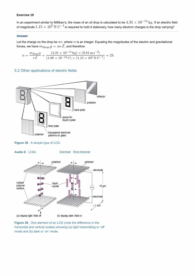
Exercise 19

In an experiment similar to Millikan’s, the mass of an oil drop is calculated to be . If an electric field

of magnitude is required to hold it stationary, how many electron charges is the drop carrying?

Answer

Let the charge on the drop be , where is an integer. Equating the magnitudes of the electric and gravitational

forces, we have , and therefore

5.2 Other applications of electric fields

Figure 35 A simple type of LCD.

Show transcriptDownloadAudio 6 LCDs

Figure 36 One element of an LCD (note the difference in the

horizontal and vertical scales) showing (a) light transmitting or ‘off’

mode and (b) dark or ‘on’ mode.

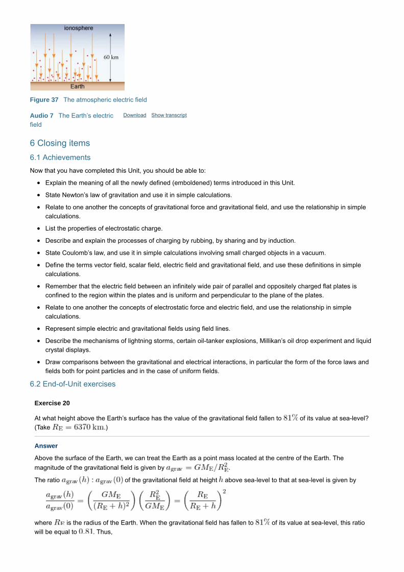
Figure 37 The atmospheric electric field

Show transcriptDownloadAudio 7 The Earth’s electric

field

6 Closing items

6.1 Achievements

Now that you have completed this Unit, you should be able to:

Explain the meaning of all the newly defined (emboldened) terms introduced in this Unit.

State Newton’s law of gravitation and use it in simple calculations.

Relate to one another the concepts of gravitational force and gravitational field, and use the relationship in simple

calculations.

List the properties of electrostatic charge.

Describe and explain the processes of charging by rubbing, by sharing and by induction.

State Coulomb’s law, and use it in simple calculations involving small charged objects in a vacuum.

Define the terms vector field, scalar field, electric field and gravitational field, and use these definitions in simple

calculations.

Remember that the electric field between an infinitely wide pair of parallel and oppositely charged flat plates is

confined to the region within the plates and is uniform and perpendicular to the plane of the plates.

Relate to one another the concepts of electrostatic force and electric field, and use the relationship in simple

calculations.

Represent simple electric and gravitational fields using field lines.

Describe the mechanisms of lightning storms, certain oil-tanker explosions, Millikan’s oil drop experiment and liquid

crystal displays.

Draw comparisons between the gravitational and electrical interactions, in particular the form of the force laws and

fields both for point particles and in the case of uniform fields.

6.2 End-of-Unit exercises

Exercise 20

At what height above the Earth’s surface has the value of the gravitational field fallen to of its value at sea-level?

(Take .)

Answer

Above the surface of the Earth, we can treat the Earth as a point mass located at the centre of the Earth. The

magnitude of the gravitational field is given by .

The ratio of the gravitational field at height above sea-level to that at sea-level is given by

where is the radius of the Earth. When the gravitational field has fallen to of its value at sea-level, this ratio

will be equal to . Thus,

So, because , .

Exercise 21

If a charged object is brought up to an insulated uncharged metal rod, the electrons in the metal flow to one end of the

rod. What causes the flow of electrons to stop?

Answer

When a charged object is brought up to an insulated metal rod, the electrons in the metal move under the influence of

the electrostatic force they experience from the charged object. Once a certain amount of excess negative charge has

built up at one end of the rod, this will itself exert an electrostatic repulsion on the other electrons in the metal and be

attracted back towards the positive charge. The flow of electrons ceases when the opposing electrostatic forces are

equal.

Exercise 22

(a) Two small conducting spheres are known to repel each other due to an electrostatic force. What can be said

about their charges?

Answer

If the two spheres repel each other, then they must carry like charges.

(b) As two small spheres are brought close together, they are found to attract each other by an electrostatic force.

What can be said about their charges? (Caution: This is not quite as easy as it may seem at first!)

Answer

If the spheres attract each other, then there are two possibilities: either (i) the spheres carry opposite charges or (ii)

one sphere is charged and the other, initially uncharged, has its charge redistributed by induction when the other

sphere gets close to it. This second situation is analogous to the attraction between a charged plastic ruler and an

uncharged piece of tissue paper. The initially uncharged sphere may be either a conductor or an insulator.

Exercise 23

If the electrostatic force on an electron at a particular point is in the direction of the positive -axis,

calculate the electric field at that point and the force on an -particle at the same point. (The charge on an -particle

is .)

Answer

The field in the -direction is given by

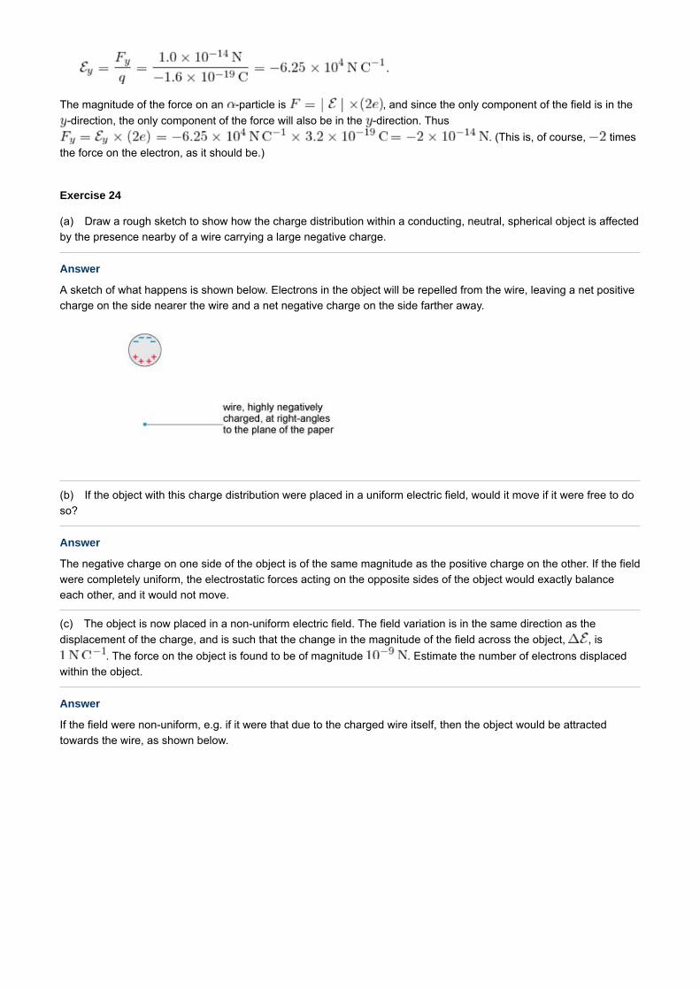
The magnitude of the force on an -particle is , and since the only component of the field is in the

-direction, the only component of the force will also be in the -direction. Thus

. (This is, of course, times

the force on the electron, as it should be.)

Exercise 24

(a) Draw a rough sketch to show how the charge distribution within a conducting, neutral, spherical object is affected

by the presence nearby of a wire carrying a large negative charge.

Answer

A sketch of what happens is shown below. Electrons in the object will be repelled from the wire, leaving a net positive

charge on the side nearer the wire and a net negative charge on the side farther away.

(b) If the object with this charge distribution were placed in a uniform electric field, would it move if it were free to do

so?

Answer

The negative charge on one side of the object is of the same magnitude as the positive charge on the other. If the field

were completely uniform, the electrostatic forces acting on the opposite sides of the object would exactly balance

each other, and it would not move.

(c) The object is now placed in a non-uniform electric field. The field variation is in the same direction as the

displacement of the charge, and is such that the change in the magnitude of the field across the object, , is

. The force on the object is found to be of magnitude . Estimate the number of electrons displaced

within the object.

Answer

If the field were non-uniform, e.g. if it were that due to the charged wire itself, then the object would be attracted

towards the wire, as shown below.

In order to estimate the number of electrons displaced, we will make the rather crude assumption that there is a

positive charge on the side near the wire and a negative charge on the other side. If the magnitude of the

electric field at the positive side of the object is then on the other side it will be and the magnitude of

the resultant force on the object will be given by

Thus

Comment: This is only a tiny fraction of the electrons available even in an object made of a material that is not a very

good conductor.

Exercise 25

In a Millikan’s oil drop type of experiment, the electric field is adjusted such that a particular drop is stationary. The

magnitude of the field is then momentarily increased and subsequently returned to its initial value. How will this affect

the motion of the droplet?

Answer

If the droplet is stationary, the gravitational and electrostatic forces must be equal and opposite. The gravitational

force is downwards, therefore the electrostatic force must be upwards. Because the droplet is negatively charged, the

electric field must be downwards. If the magnitude of the electric field is momentarily increased, there will be an

unbalanced upward force on the droplet which will give it a small upward acceleration. When the magnitude of the

field is returned to the value at which the forces balance, the droplet will continue to move upwards with the velocity it

acquired during the momentary field increase. The droplet will, of course, continue to move with a constant velocity

when the total force acting on it is zero.

6.3 Acknowledgements

Grateful acknowledgement is made to the following sources:

Animations

Animation 3-Wiring: Dmitry G. This file is licensed under the Creative Commons Attribution-Share Alike Licence

Animation 3-Man-on-beach: Original photo courtesy of Joy Manners

Animation 3-Ruler: Andy Crawford / Dorling Kindersley / Getty Images

Figures

Figure 3a: © The Art Archive/Alamy

Figure 3c: Science & Society Picture Library / SSPL / Getty Images

Figure 4: © Lebrecht Music and Arts Photo Library / Alamy

Figure 6: Wellcome Library, London. This file is licensed under the Creative Commons Attribution Licence

Figure 15: © aspenrock / 123RF

Figure 16: © INTERFOTO / Alamy

Figure 20: © Anna Omelchenko / 123RF

Figure 25: © The Hunterian, University of Glasgow 2014

Figure 28: Science & Society Picture Library / SSPL / Getty Images

Every effort has been made to contact copyright holders. If any have been inadvertently overlooked the publishers will be

pleased to make the necessary arrangements at the first opportunity.