UNIT 6 FLEXIBLE MANUFACTURING SYSTEM

6.1 Introduction

6.2 Flexibility and its type

6.3 FMS and its rule in CIM environment

6.4 Machine loading

6.5 numerical example

6.5.1 Problem description

6.5.2 Solution methodology

6.5.3 Exact heuristic by Reallocation paradigm

6.5.4 Numerical illustration

6.6 Scheduling

6.6.1 Definition

6.6.2 Dispatching rules

6.6.3 Numerical Example 6.7 Methods and practical applications

6.8 Control of FMS system

6.9 Recent trends

6.10 Summary

6.11 keywords

6.12 References

6.1 INTRODUCTION

Globalization, fickling market requirements and modern lifestyle trends have put up

tremendous challenge to manufacturing industries. In the current business scenario the

competitiveness of any manufacturing industry is determined by its ability to respond

quickly to the rapidly changing market and to produce high quality products at low costs.

However, the product cost is no longer the predominant factor affecting the

manufacturers’ perception. Other competitive factors such as flexibility, quality, efficient

delivery and customer satisfaction are drawing the equal attention. Manufacturing

industries are striving to achieve these capabilities through automation, robotics and other

innovative concepts such as just-in-time (JIT), Production planning and control (PPC),

enterprise resource planning (ERP) etc. Flexible manufacturing is a concept that allows

manufacturing systems to be built under high customized production requirements. The

issues such as reduction of inventories and market-response time to meet customer

demands, flexibility to adapt to changes in the market, reducing the cost of products and

services to grab more market shares, etc have made it almost obligatory to many firms to

switch over to flexible manufacturing systems (FMSs) as a viable means to accomplish

the above requirements while producing consistently good quality and cost effective

products. FMS is actually an automated set of numerically controlled machine tools and

material handling systems, capable of performing a wide range manufacturing operations

with quick tooling and instruction changeovers.

6.2 FLEXIBILITY AND ITS TYPES

Flexibility is an attribute that allows a mixed model manufacturing system to cope up

with a certain level of variations in part or product style, without having any interruption

in production due to changeovers between models. Flexibility measures the ability to

adapt “to a wide range of possible environment”. To be flexible, a manufacturing system

must posses the following capabilities:

Identification of the different production units to perform the correct operation

Quick changeover of operating instructions to the computer controlled production

machines

Quick changeover of physical setups of fixtures, tools and other working units

These capabilities are often difficult to engineer through manually operated

manufacturing systems. So, an automated system assisted with sensor system is required

to accomplish the needs and requirements of contemporary business milieu. Flexible

manufacturing system has come up as a viable mean to achieve these prerequisites. The

term flexible manufacturing system, or FMS, refers to a highly automated GT machine

cell, consisting of a group of computer numerical control (CNC) machine tools and

supporting workstations, interconnected by an automated material handling and storage

system, and all controlled by a distributed computer system. The reason, the FMS is

called flexible, is that it is capable of processing a variety of different part styles

simultaneously with the quick tooling and instruction changeovers. Also, quantities of

productions can be adjusted easily to changing demand patterns.

The different types of flexibility that are exhibited by manufacturing systems are given

below:

1. Machine Flexibility. It is the capability to adapt a given machine in the

system to a wide range of production operations and part styles. The greater

the range of operations and part styles the greater will be the machine

flexibility. The various factors on which machine flexibility depends are:

Setup or changeover time

Ease with which part-programs can be downloaded to machines

Tool storage capacity of machines

Skill and versatility of workers in the systems

2. Production Flexibility. It is the range of part styles that can be produced on

the systems. The range of part styles that can be produced by a manufacturing

system at moderate cost and time is determined by the process envelope. It

depends on following factors:

Machine flexibility of individual stations

Range of machine flexibilities of all stations in the system

3. Mix Flexibility. It is defined as the ability to change the product mix while

maintaining the same total production quantity that is, producing the same

parts only in different proportions. It is also known as process flexibility. Mix

flexibility provides protection against market variability by accommodating

changes in product mix due to the use of shared resources. However, high mix

variations may result in requirements for a greater number of tools, fixtures,

and other resources. Mixed flexibility depends on factors such as:

Similarity of parts in the mix

Machine flexibility

Relative work content times of parts produced

4. Product Flexibility. It refers to ability to change over to a new set of products

economically and quickly in response to the changing market requirements.

The change over time includes the time for designing, planning, tooling, and

fixturing of new products introduced in the manufacturing line-up. It depends

upon following factors:

Relatedness of new part design with the existing part family

Off-line part program preparation

Machine flexibility

5. Routing Flexibility. It can define as capacity to produce parts on alternative

workstation in case of equipment breakdowns, tool failure, and other

interruptions at any particular station. It helps in increasing throughput, in the

presence of external changes such as product mix, engineering changes, or

new product introductions. Following are the factors which decides routing

flexibility:

Similarity of parts in the mix

Similarity of workstations

Common tooling

6. Volume Flexibility. It is the ability of the system to vary the production

volumes of different products to accommodate changes in demand while

remaining profitable. It can also be termed as capacity flexibility. Factors

affecting the volume flexibility are:

Level of manual labor performing production

Amount invested in capital equipment

7. Expansion Flexibility. It is defined as the ease with which the system can be

expanded to foster total production volume. Expansion flexibility depends on

following factors:

Cost incurred in adding new workstations and trained workers

Easiness in expansion of layout

Type of part handling system used

Since flexibility is inversely proportional to the sensitivity to change, a measure of

flexibility must quantify the term “penalty of change (POC)”, which is defined as

follows:

POC = penalty x probability

Here, penalty is equal to the amount upto which the system is penalized for changes made

against the system constraints, with the given probability.

Lower the value of POC obtained, higher will be the flexibility of the system.

SAQ

1. Define flexibility. Discuss various types of flexibility?

2. Describe the essentiality of flexibility in shop floor environment?

As discussed in above section, FMS ensures quality product at lowest cost while

maintaining small lead-time. So, firms adopt FMS as a means of meeting burgeoning

requirements of customized production. Main purpose of FMS is to achieve efficiency of

well-balanced transfer line while retaining the flexibility of the job shop (Stecke, 1983,

1985). A flexible manufacturing system (FMS) has four or more processing workstations

connected mechanically by a common part handling system and electronically by a

distributed computer system. It covers a wide spectrum of manufacturing activities such

as machining, sheet metal working, welding, fabricating, scheduling and assembly.

Advantages of processes involved in flexible manufacturing system over the convectional

methods are:

Item Flexible Conventional

Set-up Defined Varies

Volume Low-Medium Medium-High

WIP (work-in-process) Low High

Flexibility High Low

Scrap Low Unpredictable

Labor Low High

Equipment cost High (short term) Low (short term)

Equipment ROI Low High

Plant ROI High Low

Queuing Low High

Automation High level Low level

Future Lead to integration Dead end

Quality Controlled Varies

Inspection Automatic tie-in Doesn’t flow

Tooling and fixturing Flexible Rigid

Market changes Flexible Rigid

6.3 FMS AND ITS RULE IN CIM ENVIRONMENT

Stable

Stable

Stable

Variable

Variable

Variable SPECIAL

SYSTEM

FMS

JOB

SHOP

Equipment utilization Optimized Low

Production control Predictable Unpredictable

Lead time Low High

Engineering changes Easier Equipment and time

constraints

Source: Modern machine shop, September 1984.

Table 6.1. Comparison between attributes of flexible and conventional manufacturing

systems

Another strategic advantage of FMS is that it is able to handle the risk caused by

uncertainty about the future. It can be done through planning in a way that maintains

flexibility of the environment. Although it is impossible to predict the future, one can

make estimates of probabilities and proceed in ways to accord with the future. The simple

decision tree in figure 6.1 illustrates the decision-making in case of FMSs governing the

choices among three different options depending upon the nature of the market.

Figure 6.1 Simple Decision Tree

100

30

90

90

45

100

The first option is a specialized manufacturing system that performs well in stable market

(payoff = 100) but will perform poorly (payoff = 30) if the market is variable. The second

option, the FMS, will perform fairly well (payoff = 90) regardless of the type of market.

The third option is the job shop that will perform well in variable (payoff = 100). From

the example it is clear that an FMS performs less well then a specific option in specific

market but proves to be a fairly good performer when the nature of market is not defined.

As a conclusion, FMS technology can be termed as an evolutionary step beyond transfer

lines that enables the industries to accommodate the growing costumer demand and

maintain the quick delivery of customized products. It is the newest wave in attaining

greater productivity with instant positive response to both adversities and new

opportunities.

TYPES OF FMS:

Flexible manufacturing systems can be divided into various types depending upon their

features. They all are discussed below:

1. DEPENDING UPON KINDS OF OPERATION-

Flexible manufacturing system can be distinguished depending upon the kinds of

operation they perform:

I. Processing operation. Such operation transforms a work material from one state

to another moving towards the final desired part or product. It adds value by

changing the geometry, properties or appearance of the starting materials.

II. Assembly operation. It involves joining of two or more component to create a

new entity which is called an assembly/subassembly. Permanent joining processes

include welding, brazing, soldering , adhesive bonding, rivets, press fitting, and

expansion fits.

2. DEPENDING UPON NUMBER OF MACHINES –

The following are typical categories of FMS according to the number of machines in

the system:

I. single machine cell (SMC). It consist of a fully automated machine capable of

unattended operations for a time period longer than one machine cycle. It is capable

of processing different part styles, responding to changes in production schedule,

and accepting new part introductions. In this case processing is sequential not

simultaneous.

II. Flexible manufacturing cell (FMC). It consists of two or three processing

workstation and a part handling system. The part handling system is connected to a

load/unload station. It is capable of simultaneous production of different parts.

III. A Flexible Manufacturing System (FMS). It has four or more processing work

stations (typically CNC machining centers or turning centers) connected

mechanically by a common part handling system and automatically by a distributed

computer system. It also includes non-processing work stations that support

production but do not directly participate in it. e.g. part / pallet washing stations, co-

ordinate measuring machines. These features significantly differentiate it from

Flexible manufacturing cell (FMC).

Figure 6.2 Comparison for three categories of FMS

3. DEPENDING UPON LEVEL OF FLEXIBILITY–

Another classification of FMS is made according to the level of flexibility associated

with the system. Two categories are distinguished here:

Annual production, Flexibility, Cost incurred.

Single machine

cell

Flexible manufacturing system

Flexible manufacturing cell

Num

ber

of

mac

hin

es

Production rate annual volume

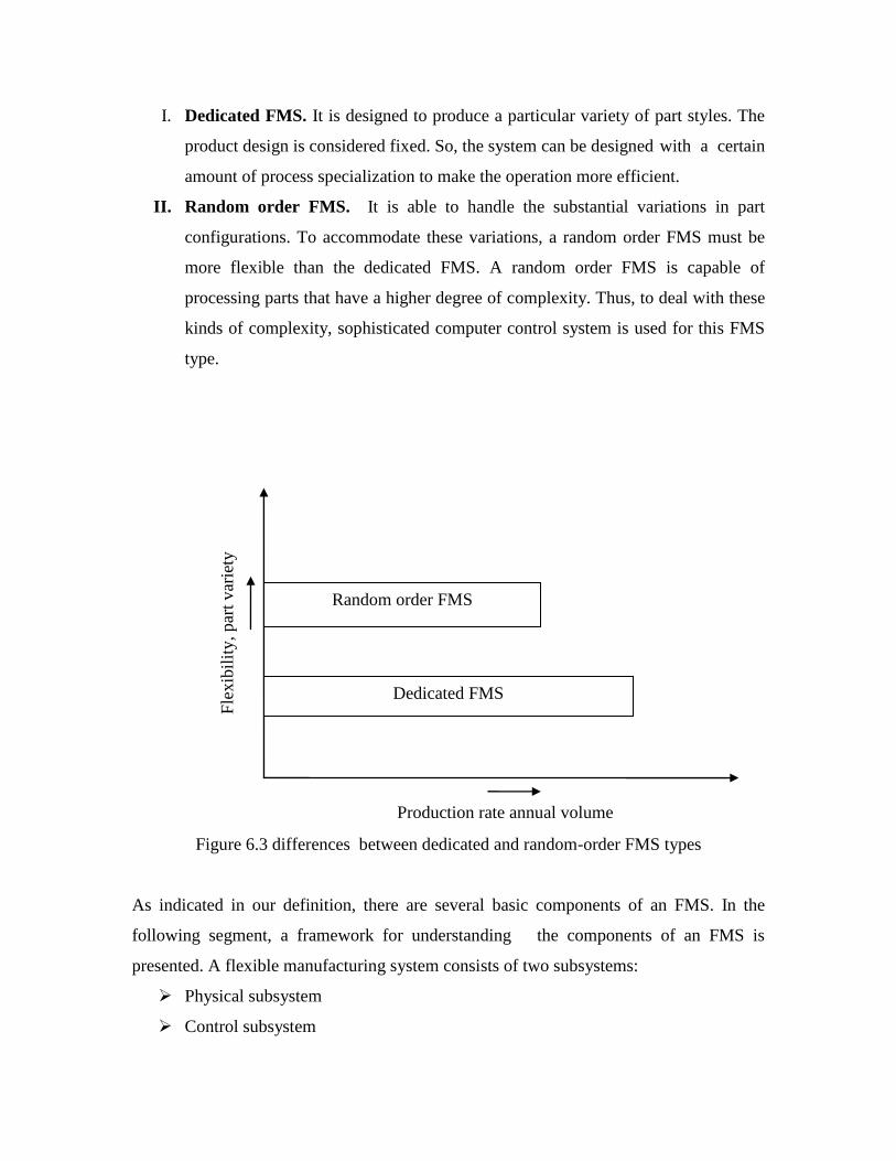
I. Dedicated FMS. It is designed to produce a particular variety of part styles. The

product design is considered fixed. So, the system can be designed with a certain

amount of process specialization to make the operation more efficient.

II. Random order FMS. It is able to handle the substantial variations in part

configurations. To accommodate these variations, a random order FMS must be

more flexible than the dedicated FMS. A random order FMS is capable of

processing parts that have a higher degree of complexity. Thus, to deal with these

kinds of complexity, sophisticated computer control system is used for this FMS

type.

Figure 6.3 differences between dedicated and random-order FMS types

As indicated in our definition, there are several basic components of an FMS. In the

following segment, a framework for understanding the components of an FMS is

presented. A flexible manufacturing system consists of two subsystems:

Physical subsystem

Control subsystem

Random order FMS

Dedicated FMS

Fle

xib

ilit

y, par

t var

iety

Physical subsystem includes the following elements:

1. Workstations. It consists of NC machines, machine-tools, inspection

equipments, loading and unloading operation, and machining area.

2. Storage-retrieval systems. It acts as a buffer during WIP (work-in-processes)

and holds devices such as carousels used to store parts temporarily between

work stations or operations.

3. Material handling systems. It consists of power vehicles, conveyers,

automated guided vehicles (AGVs), and other systems to carry parts between

workstations.

Control subsystem comprises of following elements:

1. Control hardware. It consists of mini and micro computers, programmable

logic controllers, communication networks, switching devices and others

peripheral devices such as printers and mass storage memory equipments to

enhance the working capability of the FMS systems.

2. Control software. It is a set of files and programs that are used to control the

physical subsystems. The efficiency of FMS totally depends upon the

compatibility of control hardware and control software.

Basic features of the physical components of an FMS are discussed below:

1. Numerical control machine tools.

Machine tools are considered to be the major building blocks of an FMS as

they determine the degree of flexibility and capabilities of the FMS. Some of the

features of machine tools are described below;

The majority of FMSs use horizontal and vertical spindle machines.

However, machining centers with vertical spindle machines have lesser

flexibility than horizontal machining centers.

Machining centers have numerical control on movements made in all

directions e.g. spindle movement in x, y, and z directions, rotation of

tables, tilting of table etc to ensure the high flexibility.

The machining centers are able to perform a wide variety of operations

e.g. turning, drilling, contouring etc. They consist of the pallet exchangers

interfacing with material handling devices that carry the pallets within and

between machining centers as well as automated storage and retrieval

systems.

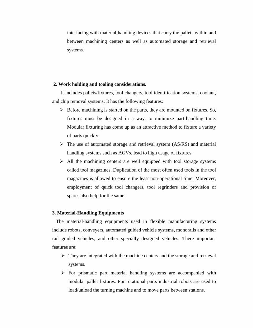
2. Work holding and tooling considerations.

It includes pallets/fixtures, tool changers, tool identification systems, coolant,

and chip removal systems. It has the following features:

Before machining is started on the parts, they are mounted on fixtures. So,

fixtures must be designed in a way, to minimize part-handling time.

Modular fixturing has come up as an attractive method to fixture a variety

of parts quickly.

The use of automated storage and retrieval system (AS/RS) and material

handling systems such as AGVs, lead to high usage of fixtures.

All the machining centers are well equipped with tool storage systems

called tool magazines. Duplication of the most often used tools in the tool

magazines is allowed to ensure the least non-operational time. Moreover,

employment of quick tool changers, tool regrinders and provision of

spares also help for the same.

3. Material-Handling Equipments

The material-handling equipments used in flexible manufacturing systems

include robots, conveyers, automated guided vehicle systems, monorails and other

rail guided vehicles, and other specially designed vehicles. There important

features are:

They are integrated with the machine centers and the storage and retrieval

systems.

For prismatic part material handling systems are accompanied with

modular pallet fixtures. For rotational parts industrial robots are used to

load/unload the turning machine and to move parts between stations.

The handling system must be capable of being controlled directly by the

computer system to direct it the various work station, load/unload stations

and storage area.

4. Inspection equipment

It includes coordinate measuring machines (CMMs) used for offline

inspection and programmed to measure dimensions, concentricity,

perpendicularity, and flatness of surfaces. The distinguishing feature of this

equipment is that it is well integrated with the machining centers.

5. Other components

It includes a central coolant and efficient chip separation system. Their features

are:

The system must be capable of recovering the coolant.

The combination of parts, fixtures, and pallets must be cleaned properly to

remove dirt and chips before operation and inspection.

SAQ

1. What do you understand by FMS? What are the components of FMS?

2. Describe the advantage of FMS over conventional manufacturing system?

3. Describe the physical sub-system of an FMS?

Operation management in an FMS is more intricate than that of the conventional

manufacturing systems e.g. transfer line or job shop production system and depends

largely upon how the decision problems is being tackled. This is primarily due to

versatile machines, which are capable of performing a wide range manufacturing

operations with quick tooling and instruction changeovers that result in many alternative

routes for processing of part types. In most FMSs, the part to be machined has to be

loaded on a pallet of some kind and after required operations; it is needed to be taken-off

from the pallets. In other words, we can say that loading involves, taking a component

6.4 MACHINE LOADING

delivered to the systems and preparing it for processing. After processing the component

is brought back from its pallet to the load/unload area and it is placed on the floor to wait

its disposal to assembly department or a storehouse. These actions come under unloading

process.

Machine loading problem of a flexible manufacturing system is known for its

complexity, which encompasses various types of flexibility aspects pertaining to part

selection and operation assignments along with constraints ranging from simple algebraic

to potentially complex and conditional one. Decision pertaining to machine loading

problems has been considered as tactical level planning decision that acts as a tie between

strategic and operating level decision in manufacturing. It receives the input from

preceding decision levels, such as part mixes selection, resource grouping, aggregate

planning, etc and transfer it to the succeeding decision levels of resources scheduling and

dynamic operation planning and control. This is why the FMS loading problems have

been rigorously pursued in the recent past.

In fact, Stecke (1983) studied machine loading problems in detail and described six main

objectives:

1. Balancing the machine processing time;

2. Minimizing the number of movement;

3. Balancing the workload per machine for a system of groups of pooled machines of

equal sizes;

4. Unbalancing the workload per machine for a system of groups of pooled machines of

unequal sizes;

5. Filling the tool magazines as densely as possible;

6. Maximizing the sum of operations priorities.

KEY TERMINOLOGIES:

1. Essential operations are those operations that can be done only on specific machine

using specific tool slots.

2. Optional operations are those operations that can be carried out on more than one

machine. It is advisable to preserve the optional operations as long as possible while

considering all possible routes. Flexibilities lie in the selection of a machine for

processing the optional operations of the part.

3. System unbalance can be defined as sum of unutilized or over-utilized time on all

machines available in the system. Maximization of machine utilization is same as

minimization of system unbalance

4. Throughput refers to the units of part types produced.

The following are provided a numerical example to illustrate the machine loading

problem clearly. Objective functions used while dealing with this problem are, the

minimization of system unbalance and the maximization of throughput because:

1) It is concerned with minimization of system idle time leading to achieve higher

machine utilizations.

2) The most important goal of any loading policy is concerned with enhancing total

system output, which is nothing but throughput.

3) Kim and Yano (1997) have found that throughput maximization by balancing the

workloads on the machine often results in limiting the tardiness.

SAQ

1. What do understand by machine loading?

2. What are the main objectives for machine loading?

3. Define the term 1) system unbalance 2) throughput 3) essential operation 4) optional

operation?

6.5 NUMERICAL EXAMPLE

6.5.1 Problem Description

Let’s consider an example of machine-loading problem of random FMS in which 8 part

types are to be processed on four machines, each having five tool slots and different

processing time for each operation. Each part type consists of essential and optional

operations, which can be performed on any of the machine without altering the sequence

of the operations. The adaptability of each machines and its potential to perform many

different operations facilitate several operation assignments to be duplicated to generate

alternative part routes. Thus, there can be fairly large number of combinations in which

operations of the part type can be assigned on the different machines while satisfying all

the technological and capacity constraints. Further consideration of flexibilities such as:

tooling flexibilities, part movement flexibilities, etc along with the constraints of the

system configuration and operational feasibility make the problem more complex.

To arrive at optimal or near optimal solution for the machine loading problem,

combinations of machines and operations allocated are evaluated using two common

performance measures: system unbalance, and throughput. It is necessary to explore each

combinatorial allocation with respect to a given objective function (minimization of

system unbalance and maximizing throughput), by simultaneously satisfying constraints.

It is found that number of possible allocations to be explored, increases exponentially as

size of the problem increases.

Part type

Operation no.

Batch size

Unit

Processing

time

Machine no.

Tool slot

needed

1

1

8

18

3

1

2 1 9 25 1 1

25 4 1

2 24 4 1

3 22 2 1

3 1 13 26 4 2

26 1 2

2 11 3 3

4 1 6 14 3 1

2 19 4 1

5 1 9 22 2 2

22 3 2

2 25 2 1

6 1 10 16 4 1

2 7 4 1

7 2 1

7 3 1

3 21 2 1

21 1 1

7 1 12 19 3 1

19 2 1

19 4 1

2 2 1 1

13 3 1

13 1 1

3 23 4 1

8 1 13 25 1 1

25 2 1

25 3 1

2 7 2 1

1 1 1

3 24 1 3

Table 6.2 Description of problem no.1 (adopted from Shanker and Srinivasulu 1989)

Many researchers have solved machine loading problems by generating the pre-

determined part sequencing based heuristics, but these techniques don’t guarantee

optimal/near optimal solutions. Therefore, the application of local intelligent search

techniques, such as genetic algorithm (GA), tabu search (TS), simulated annealing (SA),

and CBGA (Constraint Based Genetic Algorithm) have been extensively used by

researchers since 1992, to solve such a computationally complex optimization problem.

These problems have been addressed considering following objective functions:

1) Minimization of system unbalance alone;

2) Maximization of throughput alone;

3) Minimization of system unbalance and maximization of throughput considered

together;

Let us solve the above problem using an evolutionary heuristic known as Reallocation

paradigm. An approach that ensures simultaneous allocations of an index of essential as

well as optional operations on the machines based on the value “operations allocation

priority index” has been pursued. The concept of “operation allocation priority index”

(PI) has been evolved to include the effects of available and essential time and tool slots

on the machines before and after the operation decision of a part type.

6.5.2 Solution Methodology

The procedure for determining the “operation allocation priority index” of a part type can

be illustrated as follows: -

In machine loading problems, because of the availability of optional operations of part

types, decisions are to be made for allocating operations on the machines. Following

notations and definitions are to be introduced to explain the formulation of “operation

allocation priority index” (hereafter termed as priority index “PI”):.

Operation allocation: Operation allocation means the assignment of an

operation of a part type on a machine.

Op

om-operation “o” of part type “p” has been allocated to machine “m”.

Set of operations allocation: A set of operations allocation of a part type is

defined as the collection of distinct operations allocations on the machines. The

cardinality of this set is same as the total number of operations of that part type.

ASp

q = qth

set of operations allocation of part type “p”

Where “q” is the index for set of operation allocation number, q=1,2,…….qmax.

A set of operations allocation is represented as

ASp

q={Op

1m, Op

2m, Op

3m ,…………, Op

Opm’’}

m,m’,m’’,……,m’’’ {m}, where m =1 to M and m corresponds to o.

If a part type “p” contains op operations and if operation “o” can be allocated on qmax

number of machines then the total number of set of operations allocation (qmax) is given

by

qmax =

po

o 1

M m corresponds to k.

For example, the part type “7” (table 6.2), contains 3 operations, where operation 1

can be allocated on 3 machines, operation 2 on 3 machines and operation 3 on 1

machine. Therefore, the total number of sets of operation allocation that can be

formed is:

qmax =

po

p 1

mmax m corresponds to o……………………(6.1).

Where mmax is the maximum number of machine on which the operation of the part type

can be allocated.

For o =1, m =2, 3, 4, mmax =3,

For o =2, m =1, 2, 3, mmax =3,

For o =3, m =1, mmax =1,

For o =1, mmax =3,

For o =2, mmax =3,

For o =3, mmax =1, and

Op =3

nmax = 3 13 = 9.

The various set of operation allocation for this case are:-

AS17 = {O12

7, O21

7, O34

7}

AS27 = {O13

7, O21

7, O34

7}

AS37 = {O14

7, O21

7, O34

7}

…………………………………….

…………………………………….

AS97 = {O14

7, O23

7, O34

7}.

Bp is the batch size of part type “p”

tcopm is the unit processing time of operation “o” of part type “p” on machine m,

“o” corresponds to “m”.

Tcopm is the number of tool slots required for carrying out oth

operation of pth

part

type on mth

machine, “o” corresponds to “m”.

Ip is the position of part type p in the part type sequence, p = 1 to P and Ip=1 to IP

Machining time index: Corresponding to each operation allocation of a part type

on machine, the machining time index takes into account the available time on the

machine before allocation, essential time requirement of machine and available time on

machine after allocation. It represented by

MTI [Oomp] = (tropm – ETmp)/(taopm-ETmp)………………..(6.2)

Where MTI [Oomp] represents the machining time index of the machine “m” after

the allocation of operation “o” of part type “p” on machine “m” as per the nth

set of

operation allocation.

Tool Slot Index: Corresponds to each operation allocation of part type on

machine, the tool slot index takes into account the available tool slots on machine before

allocation, essential tool slot requirement of machine and available tool slots on machine

after allocation.

TSI [Oomp] = (Tropm – ESmp)/(Taopm-ESmp)………………..(6.3)

Where TSI [Oomp] represents the tool slot index of machine “m” after the allocation

operation “o” of part type “p” on machine “m” as per the nth

set of operation allocation.

• Priority Index: Priority index of set of operation allocation can be expressed as the

product of average of machining time index and tool slots index of machine. It is

represented by PI(ASqp) and expressed as:

PI(ASqp) ={1/ M

M

m 1

MTImq [Oomp ] [ 1/ M

M

m 1

TSI [ Oomp]}……(6.4)

If, TSI [ Oomp]} 0

= (Infinity), otherwise.

Table 6.3 summarizes the different situation, which can arise during the evaluation of PI

for a set of operation allocation..

Case MTImq[Oom

p] TSImp[Oom

p] PI(ASq

p) Remarks

1 All positive All positive Positive Set of operation

allocation ASp

q is

feasible.

2 Positive and

negative

All positive Positive and

negative

Set of operation

allocation ASp

q is

feasible.

3 All positive Negative Set of operation

allocation ASp

q is

infeasible.

4 Positive and

negative

Negative Set of operation

allocation ASp

q is

infeasible.

5 Negative Negative Set of operation

allocation ASp

q is

infeasible.

6 Negative All positive Negative or

Positive

Set of operation

allocation ASp

q is

feasible.

7 Positive and

negative

Positive Tropm is

Negative

Set of operation

allocation ASp

q is

infeasible.

8 Positive and

negative

All positive Positive (Tropm is

positive) but

Tropm6 < ESmp’

and Taopm <

ESmp’

Set of operation

allocation ASp

q is

feasible but given least

priority irrespective of

the value of PI(ASp

q)

Decisions pertaining to set of operation allocation is to be made based on higher PI value.

Some of the part types from the pool of part types remain unassigned due to violation of

system constraints in the given planning horizon. According to the proposed

methodology, part types are to be assigned on machines till various set of operation

allocation observes tool slot constraints (till TSI [Oomp] is positive) since overloading of

machines are permitted. After all the part from the pool of part types have been assigned,

the system unbalance indicates the termination of the throughput is to be evaluated.

Positive system unbalance indicates the termination of assignment procedure of the part

types. If the system unbalance is negative, then those part types are to be searched whose

rejection can bring system unbalance to minimum positive value with minimum

reduction in throughput. After searching such types and its subsequent rejection, the

status of machines (available time and available tool slot) are to be updated. Updation of

machine status implies addition of corresponding machining time and tool slots on the

respective machines on which the rejected part type’s operations have allocated. If any

part type has been rejected earlier on the ground of non-availability of tool slots (PI =

for all ASqp ), then the same is to be reallocated now and all other steps are repeated as

practiced for unallocated part types.

Before any part types are to assigned on machines, it is essential to determine the

sequence in which the given part types are to be allocated on the machines. Most of the

researchers have practiced standard sequencing rules such as SPT, LPT, MOPR, FIFO etc

for the determination part types sequences. Among the above sequencing rules, “SPT”

has been claimed to work better on an average. But, the determination of part type

sequence using above rules, have been viewed by several researchers as the weakness of

solution methodology for machine loading problem. Therefore, in this research, attempts

has been made to devise a part type sequencing criteria, which encompasses the several

parameters such as batch size, total processing time etc. to suit the objectives of problem.

As per the suggested criteria of part type sequencing, contribution of every part type to

these parameters is determined. Part types are to be arranged in sequence based on the

value of contribution (part types are arranged in descending order of contribution).

Contribution is to be evaluated based on the following expression:

j = (W1 p1+W2 p

2)/(W1+W2)…………………….(6.5)

Where p = Total contribution of the part types “p”.

βp1 = Contribution of the part type “p” to the batch size,

= (bp-[bp]min)/([bp]max-[bp]min)……………………………(6.6)

βp2 = Contribution of the part type “p” to the total processing time,

= ([TPTp]max- TPTp)/([TPTp]max-[TPTp]min)………………(6.7)

W1= Weightage of batch size,

W2 = weightage of total processing time,

87

88

TPTp = Total processing time of part type p

=

po

o 1

bpatop …………………………………...(6.8)

atop = Average unit processing time of operation “o” of the part type “p”

= (1/M)

M

m

p

omat1

…………………………………...(6.9)

tcopm = Unit processing time of operation “o” of the part type “p” on machine “m”.

W1= W2 = 1(For our case),

0<= βp1 <=1, 0<= βp

2 <=1, and 0< =αp <=1.

The above-mentioned concepts and logic for solving the machine-loading problem have

been summarized in the form of various steps of the exact proposed heuristic proposed in

this work. These steps are listed as follows: -

6.5.3 Exact Heuristic Reallocation paradigm

Step 1 : (1) Input the total number of part types P.

(2) Input the total number of machines M.

(3) For p=1 to P, input op,

For o=1 to pp.

For m=1 to M,

Input the value of tcopm, Tcopm o corresponds to m.

Step 2: For p =1 to P, evaluate αp using equation (6.5).

Step 3: Arrange part type p, where p=1 to P in decreasing order of the contribution αp

and generate the part type sequence.

Step 4: For p =1 to P , input the value of Ip from part type sequence.

Step 5: Input taopm, Taopm, for m=1 to M.

Step 6: Determine ETmp, ESmp for m =1 to M.

ETmp is the essential machining time requirement on machine "m" before the allocation of

any essential operation of part type

ESmp is the essential tool slot requirement on machine "m" before the allocation of any

essential operation of the part type

Step 7: Initialize Ip=1.

Step 8: Determine ASqp, the set of operation allocation of part type “p”, for q = 1 to qmax.

Step 9: Determine ERMm*, ERTm

*, ATMm

*, ATSm

*.

Where ERMm* = ETmp- ET (Oom

p)

ERTm* = ESmp –ES (Oom

p)

ATMm*=taopm – taopm(Oom

p)

ATSm*=Taopm- Taopm(Oom

p).

Step 10: Initialize q =1.

Step 11: Determine tropm, Tropm corresponding to ASqp.

Step 12: Evaluate PI (ASqp) using equation 6.4.

Step 13: If q< qmax, then q = q+1, go to step 11,

Else go to step 14.

Step 14: If for ASqp, where q = q to qmax, PI = (infinity),

then p PUTSC. Hence reject the part due to tool slot constraints, Ip = Ip +1,

go to step 8,

Else go to step 15.

Step 15: Select ASpp which has maximum PI(ASq

p) value. Allocate operation on

machines as per the (ASqp) set of operation allocation.

Step 16: Update taopm, Taopm, ETmp, and ESmp after allocation of part type “p”.

[Set tropm to taopm, Tropm to Taopm, ESmp to ESmp’ ,ESmp to ESmp

’]

Step 17: If Ip < Ip, increase Ip by 1 and go to step 8, Else go to step 18.

Step 18: Find system Unbalance “SU” and part throughput “TH”.

SU =

M

m 1

tropm and TH =

P

p 1

bp where p does not PUTSC and PUNSU.

PUTSC = Set of part types unassigned due to tool slot constraints.

PUNSU = Set of part types unassigned due to negative system unbalance.

Step 19: If SU is negative, then go for reallocation, else output the final SU and TH.

Step 20: REALLOCATION

For p =1 to P, where p does not PUTSC and PUNSU , do the following:

(A). Add TPTp to SU and SU* .

(B) Choose the minimum positive value of SU* and get the corresponding

Throughput TH* and go to step C. If SU is still negative, then add TPTp

to SU and get SU**

. Choose the minimum positive value of SU**

and

Determine the corresponding TH**

and go to step C.

(C) Reject the part type “p” from the set of assigned part types. This part type is rejected

due to negative system unbalance.

(D) Add corresponding machining time and tool slots of the part type “p” to the

respective machines. Go to step G.

(E) Reject the part type p and p* from the set of pool of assigned part types (due to part

types)

(F) Add corresponding machining time and tool slots of the allocate operations of the part

type p and p* to m respective machines. Go to step G.

(G) Allocate part type p where pPUTSC and obtain SU and TH.

(H) If SU is negative for all part types of PUTSC, reject these part types and obtain the

final SU and TH.

6.5.4 Numerical illustration

With the help of a numerical example (given in table 6.2), the details of solution

methodology using the proposed exact heuristic to address the machine loading problem

are explained in this section. For the above problem, a planning period of 8 hrs (= 480

mins) has been devised to test the computational performance of the proposed heuristic.

As a numerical illustration of the proposed heuristic, the various steps required for

solving above problem given in table 6.2 are as follows:

Step 1: (1) Total number of part types P = 8.

(2) Total number of machines M = 4.

(3) For p=1, op = 1, for p=2, op = 3, p=3, op=2, p=4 op = 2,

p=5, op = 2, for p=6, op = 3, p=7, op =3, p=8 op = 3.

(4) tc113= 18, sc113= 1

tc121= 25, tc124=25, sc121= 1, sc124=1

And remaining values can be entered from Table 6.2.

Step 2: Using equation (6.5),

α1= 0.64, α2 = 0.285, α3 = 0.71, α4 = .453, α5 = .47, α6 = .53, α7 = .508,α8 = .50

Step 3: Part type sequence: [3-1-6-7-8-5-4-2].

Step 4: Form part type sequence, I3 = 1, I1= 2, I6 = 3, I7 = 4, I8 = 5, I5 = 6,I4 = 7, I2 = 8.

Step 5: T1 = T2 = T 3 = T4 = 480,

S1 = S2 = S3 = S4 = 5.

Step 6: The values of ETmp , ESmp for m=1 to M are:

M ETmp ESmp

1 312 3

2 423 2

3 371 5

4 766 6

Step 7: I3 = 1.

Step 8: The set of operation allocation of part type “3”, for q =1 to qmax are:

AS13 = { O11

3, O23

3} and AS2

3 = { O14

3, O23

3}.

Step 9: The values of ATMm*, ATSm

*, ERMm

*, ERTm

* , for m =1 to M are:

m ATMm* ATSm

* ERMm

* ERTm

*

1 480 5 312 3

2 480 5 423 3

3 337 2 228 2

4 480 5 766 6

Step 10: Initialize q = 1.

Step 11: The values of tropm,Tropm corresponding to AS13 = { O11

3, O23

3}are:

m tropm Tropm

1 142 3

2 480 5

3 337 2

4 480 5

Step 12: Using equation 6.4, PI (AS13) = 0.373.

Step 13: qmax =2, q< qmax, then q = q+1.

Step 11: The values of tropm, Tropm corresponding to AS23= {O14

3, O23

3}are:

M tropm Tropm

1 480 5

2 480 5

3 337 2

4 142 3

Step 12: Using equation 6.4, PI (AS23) = 1.295 but Tropm6 < ESmp

’ and Taopm < ESmp’

(Case 6 of Table 6.3).

Step 13: q = qmax.

Step 14: PI (AS13) = .373 and PI (AS2

3) = 1.295 (but Tropm < ESmp

’).

Step 16: Updation

M Taopm Taopm ETmp ESmp

1 142 3 312 3

2 480 5 423 3

3 337 2 228 2

4 480 5 766 6

Step 17: I3 < I2 and I1 = 2.

Step 8: AS11 = { O13

1}

Step 9:

M ATMm*

ATSm*

ERMm*

ERTm*

1 142 3 312 3

2 480 5 423 3

3 193 1 84 1

4 480 5 766 6

Step 10: q =1.

Step 11: AS11 = { O13

1}

m Tropm Tropm

1 142 3

2 480 5

3 193 1

4 480 5

Step 13: q = qmax.

Step 15: Allocate AS11 = {O13

1}.

Step 16: Updation

m Taopm Taopm ETmp ESmp

1 142 3 312 3

2 580 5 423 3

3 193 1 84 1

4 480 5 766 1

Step 17: I6 = 3.

Step 8: AS16 = {O14

6, O22

6, O31

6}.

AS26 = {O14

6, O23

6, O31

1}.

AS36 = {O14

6, O24

6, O31

6}.

AS46 = { O14

6, O22

6, O32

6}.

AS56 = { O14

6, O23

6, O32

6}, and

AS66 = { O14

6, O24

6, O32

6}.

Step 9:

M ATMm*

ATSm* ERMm

* ERMm

*

1 142 3 312 3

2 480 5 423 3

3 193 1 84 1

4 320 4 606 5

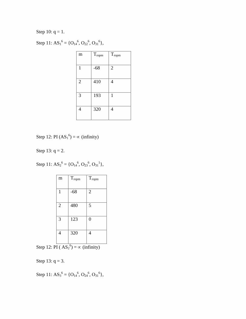
Step 10: q = 1.

Step 11: AS16 = {O14

6, O22

6, O31

6},

m Tropm Tropm

1 -68 2

2 410 4

3 193 1

4 320 4

Step 12: PI (AS16) = (infinity)

Step 13: q = 2.

Step 11: AS26 = {O14

6, O23

6, O31

1},

m Tropm Tropm

1 -68 2

2 480 5

3 123 0

4 320 4

Step 12: PI ( AS26) = (infinity)

Step 13: q = 3.

Step 11: AS36 = {O14

6, O24

6, O31

6},

m Tropm Tropm

1 -68 2

2 480 5

3 193 1

4 250 3

Step 12: PI ( AS36) = (infinity).

Step 13: q = 4.

Step 11: AS46 = { O14

6, O22

6, O32

6}.

M tropm Tropm

1 142 3

2 200 3

3 193 1

4 320 4

Step 12: PI(AS46) = 0.413.

Step 13: q = 5.

Step 11: AS56 = { O14

6, O23

6, O32

6},

M Tropm Tropm

1 142 3

2 270 4

3 193 1

4 250 3

Step 12: PI (AS56}= 1.725.

Step 13: q = 6.

Step 11: AS66 = { O14

6, O24

6, O32

6}.

M tropm Tropm

1 142 3

2 270 4

3 193 1

4 250 3

Step12: PI (AS66) = 1.665.

Step 13: q = qmax = 6.

Step 14: PI (AS46) = .413, PI (AS5

6) = 1.725, PI (AS6

6) = 1.665.

Step 15: Select AS56

as PI (AS56) = 1.725.

Step 16: Updation.

m taopm Taopm ETmp ESmp

1 142 3 312 3

2 270 4 423 3

3 123 0 84 1

4 320 4 606 5

Step 17: I7 = 4.

Step 8: AS17 = { O12

7, O21

7, O34

7},

AS27 = { O12

7, O22

7, O34

7},

AS37 = { O12

7, O23

7, O34

7},

AS47 = { O13

7, O21

7, O34

7},

AS57 = { O13

7, O22

7, O34

7},

AS67 = { O13

7, O23

7, O34

7},

AS77 = { O14

7, O22

7, O34

7},

AS87 = { O14

7, O22

7, O34

7}.

AS97 = { O14

7, O22

7, O34

7}.

Step 9:

M ATMm*

ATSm*

ERMm*

ERTm*

1 142 3 312 3

2 270 4 423 3

3 123 0 84 1

4 44 1 333 2

Step 10: q = 1.

Note: Step 11-13 involves repetitive calculations, therefore results are summarized

below:

PI(AS17)

=

PI(AS27)

=

PI(AS37)

=

PI(AS47)

=

PI(AS57)

=

PI(AS67)

=

PI(AS77)

=

PI(AS87)

= 0.5537 and,

PI(AS97)

=

Step 14: Select AS87 as PI(AS8

7) = 0.5537.

M tropm Taopm

1 142 3

2 114 3

3 123 0

4 -184 0

Step 16: Updation

M taopm Taopm ETmp ESmp

1 142 3 312 3

2 114 3 423 3

3 123 0 84 1

4 -184 0 333 2

Step 17: I8 = 5.

Step 8: AS18 = { O11

8, O22

8, O31

8},

AS28 = { O11

8, O21

8, O31

8},

AS38 = { O12

8, O22

8, O31

8},

AS48 = { O12

8, O21

8, O31

8},

AS58 = { O13

8, O22

8, O31

8} and,

AS68 = { O13

8, O21

8, O31

8}.

Step 9:

M ATMm*

ATSm*

ERMm*

ERTm*

1 -170 0 0 0

2 114 3 423 3

3 123 0 84 1

4 -184 0 333 2

Step 10: q = 1

Note: Step 11-13 involves repetitive calculations; therefore the calculated results

are summarized below:

PI(AS18) =

PI(A218) =

PI(A318) = α

PI(AS48) = 1.0048

PI(AS58) =

PI(AS68) =

Step 14: For AS48 , PI (AS4

8) = 1.0048.

Step 15: AS48

is selected.

Step 16: Updation

m taopm Taopm ETmp ESmp

1 -170 0 0 0

2 -306 1 423 3

3 123 0 84 1

4 -184 0 333 2

Step 17: I5 = 6.

Step 8: AS15 = {O12

5, O22

5},

AS25 = {O13

5, O22

5}.

Step 9:

m ATMm*

ATSm*

ERMm*

ERTm*

1 -170 0 0 0

2 -153 0 198 2

3 123 0 84 1

4 -184 0 333 2

Step 10: q = 1

Note: Step 11-13 involves repetitive calculations; therefore the calculated results

are summarized below:

PI(AS15) =

PI(AS25) =

Step 14: For every ASj5, the value PI = α. Part type 5 is rejected due to tool slot

constraints and I4 = 7

Step 8: AS14 = { O13

5, O24

5 }.

Step 9:

m ATMm*

ATSm*

ERMm*

ERTm*

1 -170 0 0 0

2 -306 1 423 3

3 -39 -1 0 0

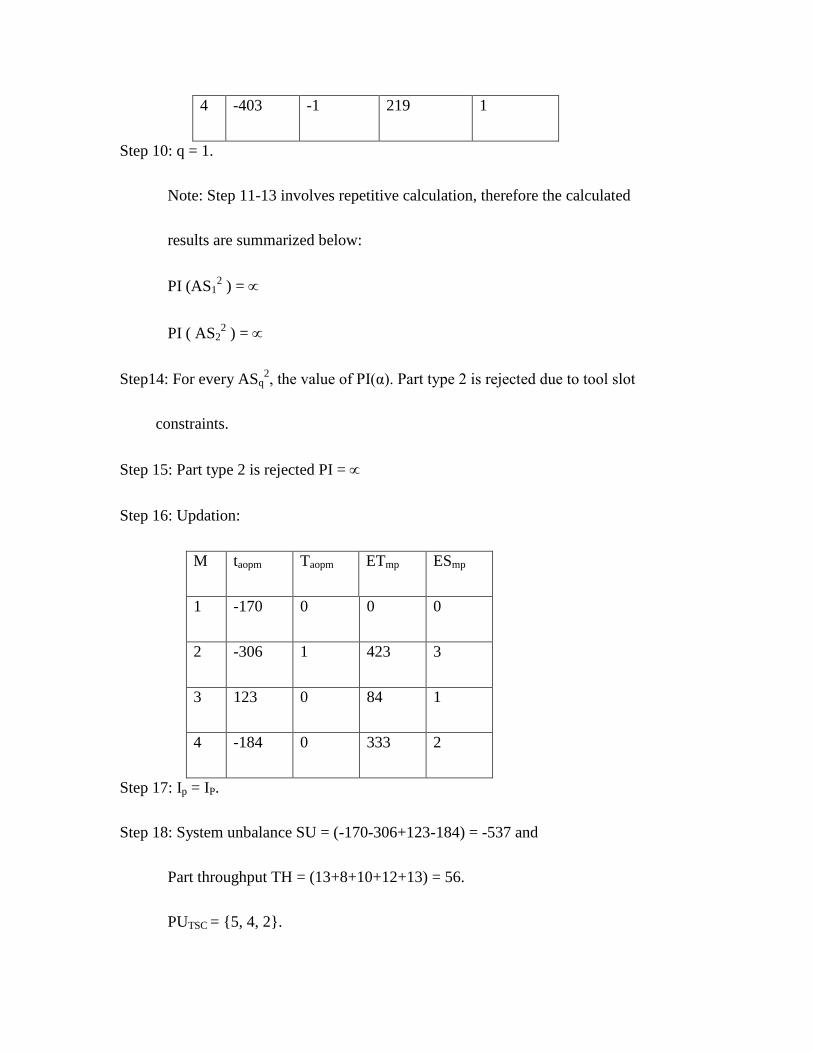
4 -403 -1 219 1

Step 10: q = 1.

Note: Step 11-13 involves repetitive calculation, therefore the calculated

results are summarized below:

PI (AS12 ) =

PI ( AS22 ) =

Step14: For every ASq2, the value of PI(α). Part type 2 is rejected due to tool slot

constraints.

Step 15: Part type 2 is rejected PI =

Step 16: Updation:

M taopm Taopm ETmp ESmp

1 -170 0 0 0

2 -306 1 423 3

3 123 0 84 1

4 -184 0 333 2

Step 17: Ip = IP.

Step 18: System unbalance SU = (-170-306+123-184) = -537 and

Part throughput TH = (13+8+10+12+13) = 56.

PUTSC = {5, 4, 2}.

Step 19: system unbalance is negative so go for reallocation.

Step 20: Reallocation.

(A). For p = 1, ,3, 6, 7, and 8 , where pPUTSC and PUNSU, add TPTp to SU

and get SU*.

(B) The minimum positive value of SU* = 123 is obtained by adding TPT7 = 660 and

the corresponding throughput TH* = 44.

(C) Reject the part type 7 from the set of pool of assigned part types. This part type is

rejected due to negative system unbalance. PUNSU = {7}.

(D) Corresponding machining time and tool slots of the allocated operations of part

type 7 is added to the respective machines.

Updation:

m taopm Taopm ETmp ESmp

1 58 1 0 0

2 -150 2 423 3

3 123 0 84 1

4 92 3 333 2

(G) Reallocated part type 5, 4, and 2.

Part type 5 cannot be allocated due to Tool Slot Constraints [PI (AS15) =

and PI(AS25) = .]

Part type 4 cannot be reallocated due to Tool Slot Constraints [PI (AS14) = ]

Part type 2 can be reallocated and the updated status is as follows:

m taopm Taopm ETmp ESmp

1 -167 0 0 0

2 -348 1 225 2

3 123 0 84 1

4 -124 2 117 1

SU = -516 and TH = 53

(H) The SU is negative for all part types of PUTSC, and hence reject part type and

Finally System Unbalance SU = 123 and throughput TH = 44, PUNSU ={7}.

PUTSC = {5, 4, 2}.

SAQ

1. What are the different steps involved in the Reallocation paradigm?

2. define tool slot index and priority index?

6.6 SCHEDULING

6.6.1 DEFINITION

Scheduling is a process of adding start and finish time information to the job order

dictated in the sequencing process. Sequencing process in turn, is defined as getting the

order in which jobs are to be run on a machine. The sequence thus obtained determines

the schedule, since we assume each job is started on the machine as soon as the job has

finished all predecessor operations and the machine has completed all earlier jobs in the

sequences. This is referred to as semi-active schedule and acts as an optimal policy for

minimizing the completion time, flow time, lateness, tardiness, and other measures of

performance. Scheduling problems are often denoted by N/ M/ F/ P, where N is the

number of jobs to be scheduled, M is the number of machines, F refers to the job flow

pattern, and P is performance measures that are to be appropriately minimized or

maximized. The solution of scheduling problems are generally presented in the form of

gannt-chart which is a chart plotted between different work centers and total processing

time on that work center. Following is given an example problem to illustrate the

formation of Gantt-chart.

Example 6.1. Consider a set of jobs and processing times shown in table 6.4 generate

the schedule assuming jobs are processed in the order {2, 4, 1, 3}

station

Job 1 2 3 4

1 2.0 3.5 1.5 2.0

2 4.5 3.0 2.5 1.0

3 1.5 1.5 5.0 0.5

4 4.0 1.0 2.5 0.5

Table 6.4 flow shop processing time

Solution.

We start by assigning job 2 on station 1 at time t=0. Since p21 = 4.5, the operation last on

station 1 for 4.5 unit time. Since all the operation starts with station 1 thus in that

particular time rest station are in idle condition. At time when job 2 is moved to station 2

then job 4 move to station 1 for processing and other jobs remain in the buffer. Station 2

finishes operation 2, when P22 = 3.0 time units later (time is now t=7.5). Station 1 is still

busy with job 4; thus, while job 2 is begun on station 3, station 2 is idle, waiting for job 4

to be completed on station 1. Similarly, the process continues till processing of the entire

job takes place. The result is given in figure 6.4 through a Gantt chart. The gap in

between two bars represents idle time.

Figure 6.4 Gantt chart for above example

In a flow shop all N jobs is made to visit machines in the same sequence. Suppose we

also restrict our solutions in such a way that all machines process jobs in the same order,

then it will refer to as permutation schedule. In this case, at time t=0, the first job is

started on machine 1 and as soon as this operation is completed the first job begins on

machine 2 and the second job begins on machine 1. This process is continued until the

last job finishes on machine M. the benefit of this process is that we have to consider only

N! Sequence instead of (N!)M

.

6.6.2 Dispatching Rules

When a processing unit gets ready, a job must be selected from its input queue for

immediate setup and processing. This refers to as dispatching. Dispatching rules are

generally classified as being static or dynamic. Static rules are those that stay constant as

jobs travel through the plant, e.g. LTWK, EDD where as dynamic rules are those that

2 4 1 3

2 4 1 3

2 3 2 4

2 4 1 3

5 10 15 20

Time

Pro

cess

or

4

3

2

1

changes with time and queue characteristic e.g. LWKR. Sometimes dispatching rules are

also distinguished as myopic or global. Myopic rules look only at the individual machine

e.g. SPT where as global rules look at the entire shop e.g. WINQ.

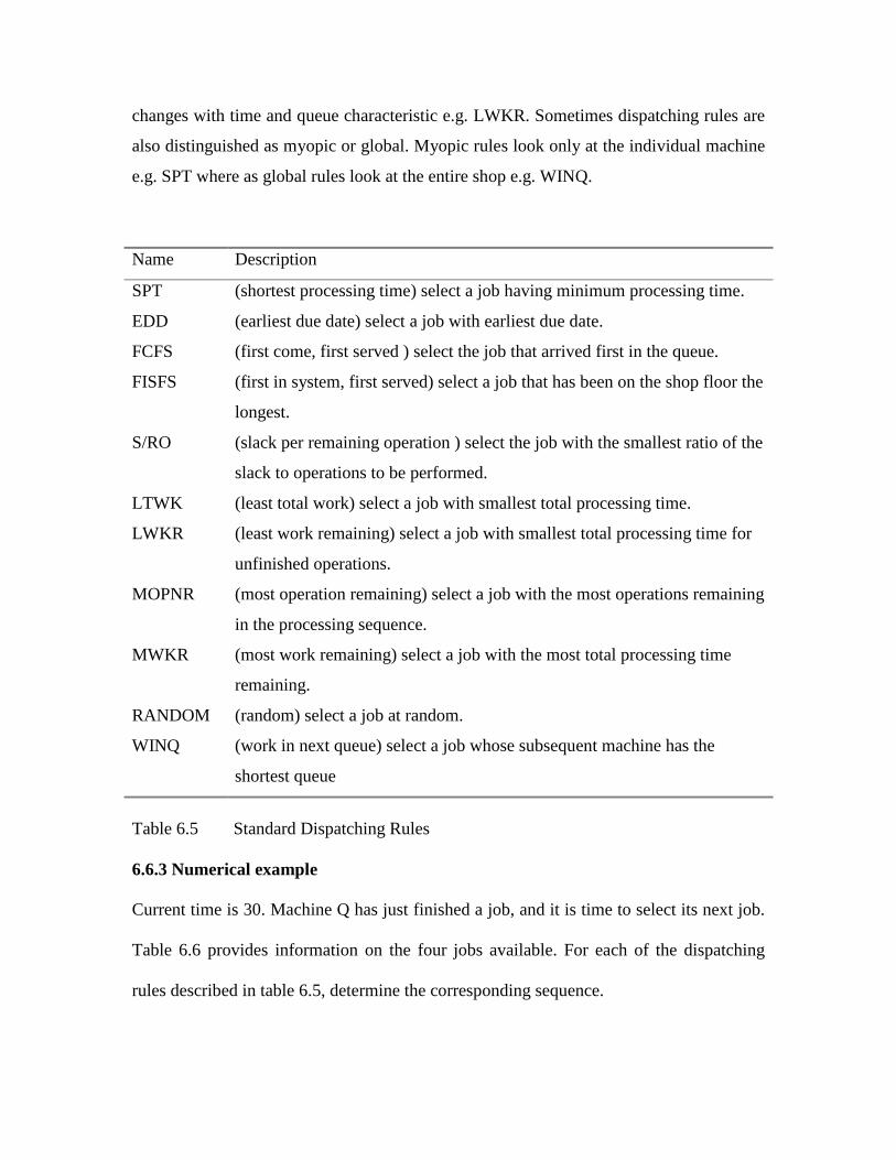
Name Description

SPT (shortest processing time) select a job having minimum processing time.

EDD (earliest due date) select a job with earliest due date.

FCFS (first come, first served ) select the job that arrived first in the queue.

FISFS (first in system, first served) select a job that has been on the shop floor the

longest.

S/RO (slack per remaining operation ) select the job with the smallest ratio of the

slack to operations to be performed.

LTWK (least total work) select a job with smallest total processing time.

LWKR (least work remaining) select a job with smallest total processing time for

unfinished operations.

MOPNR (most operation remaining) select a job with the most operations remaining

in the processing sequence.

MWKR (most work remaining) select a job with the most total processing time

remaining.

RANDOM (random) select a job at random.

WINQ (work in next queue) select a job whose subsequent machine has the

shortest queue

Table 6.5 Standard Dispatching Rules

6.6.3 Numerical example

Current time is 30. Machine Q has just finished a job, and it is time to select its next job.

Table 6.6 provides information on the four jobs available. For each of the dispatching

rules described in table 6.5, determine the corresponding sequence.

Operation (machine Pi,j)

Job

Arrival to

the system

Arrival at

Q

Due date 1 2 3

1 5 10 30 (Q,5) (P,1) (S,6)

2 0 5 20 (P,5) (Q,3) (R,2)

3 9 9 10 (R,3) (S,2) (Q,2)

4 0 8 25 (T,6) (Q,4) (R,4)

Table 6.6 Machine-Job data

Solution.

SPT: job {1,2,3,4} have processing time of {5,3,2,4} on machine Q. placing job in

increasing order of processing time yield the job sequence {3,2,4,1}. Thus, load job 3

into machine Q.

EDD: job {1, 2, 3, 4} have due date {30, 20, 10, 25}, respectively. Ordering by due

earliest due dates we get sequence {3, 2, 4, 1}.

FCFS: jobs arrived at Q at times {10, 5, 9, 8}. Placing earlier arrival time first, we obtain

a sequence {2, 4, 3, 1}.

FISFS: jobs arrived the system at {5, 0, 9, 0}. In this case job 2 and 4 can be arranged

arbitrary thus we get 2 sequences {2,4,1,3} and {4,2,1,3}.

S/RO: slack = (due date – current time – remaining processing time).

S/RO = slack/remaining operations.

Slacks for job 1,2,3,4 are as follows:

For job 1 = (30 – 10 – 5 – 1 – 6) = 8

For job 2 = (20 – 10 – 3 – 2) = 5

For job 3 = (10 – 10 – 2) = -2

For job 4 = (25 – 10 – 4 – 4) = 7.

S/RO for jobs is

For job 1 = 8/3 = 2.67

For job 2 = 5/2 = 2.50

For job 3 = -2/1 = -2

For job 4 = 7/2 =3.50

Placing the job in the increasing order of S/RO we get the sequence {3, 2, 1, 4}

LTWK: total work can be calculated by adding all the processing time.

Thus remaining work on jobs are {12, 10, 7, 14}. Arranging by the total work values we

get sequence {3, 2, 1, 4}.

LWKR: remaining workload until job completion is {12, 5, 2, 8}. The corresponding

sequence is {3, 2, 4, 1}.

MOPNR: Numbers of remaining operation are {3, 2, 1, 2}. Applying MONPR we get

sequence {1, 2, 4, 3}.

MWKR: remaining processing time are {12, 5, 2, 8}. The sequence obtained is {1, 4, 2,

3}.

RANDOM: selecting the job randomly we get {1, 4, 3, 2}.

WINQ: let the length of the queue are 12 at machine P and 6 at machine R. job 3 goes

first since it has no next queue. Jobs 2 and 4 come next since they are headed for machine

R, which has less work in its queue that P. thus, the sequence obtained is {3,2,4,1}

SAQ

Problem 6.1. What do you understand by scheduling?

Problem 6.2. Define dispatching and name different types of dispatching rule?

Problem 6.3. Current time is 30. Machine A has just finished a job, and it is time to

select its next job. Table 6.7 Provide information on the five jobs available. For each of

the dispatching rules described in table 6.5, determine the corresponding sequence.

Table 6.7 Machine-Job data

6.7 METHODS AND PRACTICAL APPLICATIONS

The concept of flexible automaton is applicable to a variety of manufacturing operations.

In this section, some practical applications of flexible manufacturing systems are

presented and their layouts are provided:

Operation (machine Pi,j)

Job

Arrival to

the

system

Arrival at

A

Due date 1 2 3

1 3 7 29 (A,6) (B,2) (D,8)

2 5 9 23 (C,2) (A,3) (D,1)

3 9 3 18 (A,3) (C,5) (D,5)

4 8 7 13 (D,6) (C,6) (A,3)

5 0 5 12 (E,4) (A,5) (C,3)

1. System with linear track. Systems having linear tracks usually have only one

vehicle. Most frequently used vehicle in such systems is rail-guided vehicle;

however an AGV can also be used. The physical layout of a simple FMS with

linear track, employed at Andreson Strathclyde plc12

, in Motherwell, near

Glasgow in Scotland, is given in figure 6.5. There are five machines, each

with a tool magazine of 100 tools capacity. Four of them are identical, while

fifth one has facing head, required for certain operations. Each machine has

two pallet stands providing on-queue and off-queue buffers. The load/unload

area constitute two pallet stands and some work stands, where the part is put

into the fixture, before putting it on the pallet at one of the pallet stands. There

are 13 identical pallets, and an AGV that can handle one pallet at a time and

travel through a track with no branches.

Figure. 6.5. Layout of Andreson Strathclyde FMS

The major problem with this particular kind of system is that, there are no places for

storing the pallets with part-machined components except pallet stands at the machine

centers and load/unload area.

2. Systems with AGV networks.

Whenever a system track consists of networks of loops and branches, AGVs are

employed. Systems with AGV networks have generally more than one vehicle. However,

if the workload is too low, one vehicle is sufficient to cope with the traffic. A system

Load/unload

area

Machining

Centre

Machining

Centre

Machining

Centre

Machining

Centre

AGV Track for

AGV

Layout Detail

which illustrates this arrangement is the FMS cell at Cincinnati Milacron in Birmingham,

England and is shown in figure 6.6 It has two machining centers with pallet shuttles, a

wash machine, a co-ordinate measuring machine, and two load/unload stations.

<< Include scanned Figure 6.6 >>

Figure 6.6 Line diagram for an FMS used by Cincinnati Milacron Plastics Machinery

Division

3. Systems with number of distinct cells.

Such systems consist of a number of distinct sub-divisions or cells, each of which has

some characteristics of an FMS. One example is the Holset engineering in Huddersfield

that has installed a system consisting of seven cells for the manufacture of shaft and

wheel assemblies for their turbochargers18.32

. The layout of the system is shown in figure

6.7. The manufacturing sequence is split into self-contained stages and a cell created to

perform the operation of that stage. The operation involves machining, welding,

hardening and tempering, grinding and balancing. Within each cell there are two pallet

stands from which parts are moved among workstations using gantry robot. It also

consists of a storehouse for storing raw materials, and semi-finished and finished

components.

Figure 6.7.Layout of cells in Holset engineering FMS (courtesy Holset engineering Ltd.)

The system is designed to allow each cell to operate independently, so that the effects of

any possible breakdown could be minimized.

1

2

3

4

5

6

7

Sto

res

Input

parameter

Output

variable

6.8 CONTROL OF FMS SYSTEM

The FMS includes a distributed computer system that is linked to the work stations,

material handling system and other hardware components. A typical FMS computer

system consists of a central computer and micro computers controlling the individual

machines and other components. The control system in FMS causes the process to

accomplish its defined function. The control can be either closed loop or open loop. A

closed loop control system is one in which the output variable is compared with an input

parameter and any difference between the two is used to drive the output into agreement

with the input. It is also known as feedback control system. A closed loop control system

consists of six basic elements which is shown in figure 6.8

Figure 6.8 A Feedback control system

Here, the controller compares the output value with the input and makes the required

adjustment in the process to reduce the difference between them, which is accomplished

by actuators. Actuators are the hardware devices that physically carried out the control

Feed back

sensor

Controller Actuator Process

Input

parameter

Output

variable

actions such as an electric motor, electric fan. A sensor is used to measure the output

variable and closed the loop between input and output.

In contrast to the closed loop control system an open loop operates without the feedback

loop as in figure 6.9

Figure 6.9 An open loop control system

Its advantage is that it is generally simpler and lesser expensive then a closed loop

system. Open loop system is usually appropriate to use when (1) the actions performed

by the control system are simple. (2) The actuating function is very reliable and (3) any

reaction forces opposing the actuation are negligible to effect the actuation. Functions

performed by the FMS computer control system can be grouped into the following

categories:

Workstation control. In a fully automated FMS, a computer control system is

used at the individual processing or assembly stations.

Distribution of control instructions to workstations. DNC is used for this

purpose. The DNC system stores the programs, allows submission of new

programs and editing of existing programs as needed.

Production control. The production control functions are accomplished by

routing and applicable pallet to the load/ unload area and providing instructions to

the operator for loading the desired work part.

Material handling control. It is accomplished by actuating switches at branches

and merging points, stopping parts at machine tool transfer location, and moving

pallets to load/ unload stations.

Tool control. It is concerned with managing mainly two aspects of the machine

tool,

Controller Actuator Process

Tool locations i.e. Keeping track of the machine tools at each work-

station by receiving the information that whether tools required to process

to particular work piece is present at the station or not.

Tool life monitoring deals with the idea that whether the cumulative

machining time is below the specified tool life or not. In case machining

time reaches the specified life of the tool, the operator is notified that a

tool replacement is needed.

Performance evaluation. The computer system is programmed to collect data on

the operation and the performance of the FMS. This data is then periodically

summarized to report to the management system.

6.9 RECENT TRENDS

Depending upon the problem environment, many new trends have been accommodated

with FMS to accord with the requirements of highly customized production, high

flexibility, low production cost, and low lead time. Some of these recent developments in

the field of manufacturing sector made in order to stack up against the competitive

market scenario are given below:

1) Production planning and control (PPC). It is concerned with the logistic problems

that are encountered in manufacturing processes. It includes the details of what

and how many products to produce and when to obtain the raw materials, parts

and resources to produce those products.

2) Master production schedule (MPS). It is a list of the product to be manufactured,

when they should be completed and delivered, and in what quantities. The master

schedule must be based on an accurate of demand and realistic assessment of the

company’s production capacity.

3) Material requirements planning (MRP). It is a planning technique, usually

implemented by computer, that translates the MPS of end products into a detailed

scheduled for the raw materials and parts used in those end products. MRP is

often thought of as a method of inventory control. However its implementation is

complicated due to the sheer magnitude of data to be processed. For example

several component may be made out of the same gauge sheet metal the

component are assembled into simple sub assemblies, and these sub assemblies

are put together into more complex sub assemblies, and so on, until the final

products are assembled. Each step in the manufacturing and assembly sequence

takes time. All of these factors must be incorporated into the MRP calculations

which make it a complicated one.

4) Just in time (JIT). It refers to a scheduling discipline in which materials and parts

are delivered to the next production line station just prior to their being used. In

this type of discipline tends to reduce inventory and other kinds of waste

manufacturing. The ideal JIT production system produces and delivers exactly the

required number of each component to the down stream operation in the

manufacturing sequence just at the time when that component is needed.

5) Manufacturing resource planning (MRP II). It is defined as a computer based

system for planning, scheduling, and controlling the materials, resources, and

supporting activities needed to meet the MPS. The recent generations of MRP II

such as enterprise resource planning (ERP), manufacturing execution system

(MES), customer oriented manufacturing management systems (COMMS) etc

have found great applications in the areas of quality control, maintenance

management, customer field service, supply chain management, and product data

management.

6) E-manufacturing. In the modern manufacturing system internet has enabled the

manufacturers in such a way that the lead time of the manufacturing of the

products have come down and the quality of the product has been enhanced.

6.10 SUMMARY

The flexible manufacturing system is a manufacturing concept for mid-volume, mid-

variety part production. There could be a number of FMS’s configurations possible

depending upon its feature such as number of machines, kinds of operation, and level of

flexibility designed into the system. Further more, the degree of automation of the

machine tools, material handling systems and central computer system, depends on the

objectives of an organization.

An FMS is capable of accommodating engineering and process changes that are liable to

occur during manufacturing. In this chapter, various aspects of FMS such as physical and

control components, its types, and some analytical treatments of machine loading

problems, scheduling problems is illustrated to characterize its supremacy over the other

conventional manufacturing system.

6.11 KEYWORDS

Flexibility , Penalty of change (POC), System Unbalance (SU), Throughput (TH),

Reallocation Paradigm, Priority Index (PI), essential operations, optional operations,

shortest processing time (SPT), earliest due date( EDD), first come first served (FCFS),

first in system first served (FISFS), slack per remaining operation (S/RO) , least total

work (LTWK) , least work remaining (LWOR), most operation remaining (MOR), most

work remaining (MWKR), random(RANDOM), work in next queue (WINQ), Production

planning and control (PPC), Master production schedule (MPS), Material requirements

planning (MRP), Just in time (JIT), Manufacturing resource planning (MRP II).

6.11 REFERENCES

ASKIN R. G., and STANDRIDGE C. R., 1993 “Modeling and Analysis of

Manufacturing Systems”. John Wiley and Sons, Inc.

GROOVER, M. P., 2001. “Automation, Production Systems, and Computer-Integrated

Manufacturing, 2nd

Ed”. Pearson education, Singapore.

KIM, Y. D., and YANO, C. A., 1997, Impact of throughput based objectives and

machine grouping decisions on the short-term performance of flexible manufacturing

system, International Journal of Production Research, 35 (2), 3303-3322.

SHANKAR, K., and SRINIVASULU, A., 1989, Some solution methodologies for

loading problems in flexible manufacturing system, International Journal of Production

Research, 27 (6), 1019-1034.

SINGH, N., 1996, “Systems approach to computer-integrated design and manufacturing”.

John Wiley and Sons, Inc.

STECKE, K.E., 1983, Formulation and solution of non-linear integer production

planning problem for flexible manufacturing system, Management Science, 29(3), 273-

288.

STECKE, K.E., 1985, A hierarchical approach to solving grouping and loading problems

of flexible manufacturing systems, European Journal of operational Research, 24(3),

369-378.