Embed Size (px)
Citation preview
UNIT - 6
Applying Structure to Hadoop Data with Hive
In This Chapter▶ Introducing Hive
▶ Exploring the Hive architecture
▶ Getting started (properly) with Hive
▶ Working with the Hive clients
▶ Seeing which data types work with Hive
▶ Creating and managing databases and tables
▶ Mastering the Hive data-manipulation language
▶ Querying and analyzing data
If you were to look back at the history of the IT Industry, you’d soon see that every decade has had one or more watershed moments. Huge inno-
vations have often dramatically impacted the industry as a whole, changing the course of certain companies and creating a “genesis moment” for others. Edgar F. Codd’s groundbreaking work in the 1970s on the relational model that spawned the whole relational database management system (RDBMS) industry was definitely a significant innovation. Immediately following Codd’s innovation was the introduction of structured query language (SQL), which was created by Donald D. Chamberlin and Raymond F. Boyce to provide a common programming language for managing data stored in a RDBMS. The RDBMS and SQL technologies became the de facto standards for data man-agement and processing and have continued to hold sway over the industry.
Now, if you were to ask us to name the major innovation of the “noughties” (we’re still getting used to this nickname for the aught years, from 2000 to 2009), we’d pick Apache Hadoop, of course — the amazing new technol-ogy for big data management, analysis, and processing. However, few if any new IT technologies, no matter how innovative and attractive, can uproot
228 Part III: Hadoop and Structured Data
established standards and start over with a clean slate. For Hadoop to truly have a broad impact on the IT Industry and live up to its true potential, it needed to “play nice” with the older technologies: It had to support SQL; integrate with, and extend, the RDBMS; and enable IT professionals who lack skills in using Java MapReduce to take advantage of its features. For this reason (and others, which we discuss later in this chapter), Apache Hive was created at Facebook by a team of engineers who were led by Jeff Hammerbacher. Hive, a top-level Apache project and a vital component within the Apache Hadoop ecosystem, drives several leading big-data use cases and has brought Hadoop into data centers across the globe.
Saying Hello to HiveTo make a long story short, Hive provides Hadoop with a bridge to the RDBMS world and provides an SQL dialect known as Hive Query Language (HiveQL), which can be used to perform SQL-like tasks. That’s the big news, but there’s more to Hive than meets the eye, as they say, or more applica-tions of this new technology than you can present in a standard elevator pitch. For example, Hive also makes possible the concept known as enter-prise data warehouse (EDW) augmentation, a leading use case for Apache Hadoop, where data warehouses are set up as RDBMSs built specifically for data analysis and reporting. Now, some experts will argue that Hadoop (with Hive, HBase, Sqoop, and its assorted buddies) can replace the EDW, but we disagree. We believe that Apache Hadoop is a great addition to the enterprise and that it can augment (as mentioned earlier in this paragraph) and comple-ment existing EDWs. This particular debate is also the subject of Chapter 10, so check out our discussion there. For now, we leave that debate alone and simply explain in this chapter how Hive, HBase, and Sqoop enable EDW augmentation.
Closely associated with RDBMS/EDW technology is extract, transform, and load (ETL) technology. To grasp what ETL does, it helps to know that, in many use cases, data cannot be immediately loaded into the relational database — it must first be extracted from its native source, transformed into an appropriate format, and then loaded into the RDBMS or EDW. For example, a company or an organization might extract unstructured text data from an Internet forum, transform the data into a structured format that’s both valuable and useful, and then load the structured data into its EDW.
As you make your way through this chapter (if you choose to read it that way), you can see that Hive is a powerful ETL tool in its own right, along with the major player in this realm: Apache Pig. (See Chapter 8 for more on Apache’s porcine offering.) Again, users may try to set up Hive and Pig as the new ETL tools for the data center. (Let them try.) As with the debate over
229 Chapter 13: Applying Structure to Hadoop Data with Hive
EDW versus Apache Hadoop, we see these Apache Hadoop technologies not as direct replacements for existing ETL tools but instead as powerful new ETL tools to be used when appropriate.
Last but not least, Apache Hive gives you powerful analytical tools, all within the framework of HiveQL. These tools should look and feel quite familiar to IT professionals who understand how to use SQL. We provide you with hands-on examples of Hive analytics later in this chapter, but first we discuss the architecture of Hive in the next section.
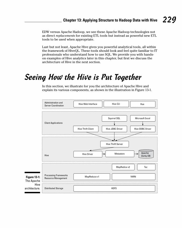
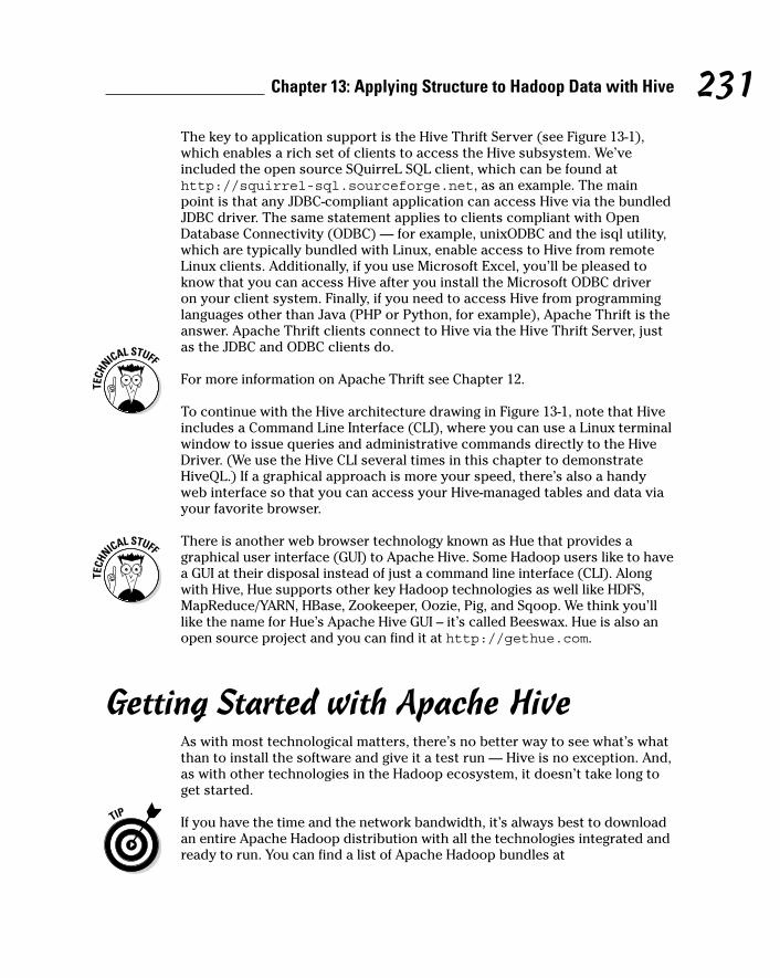
Seeing How the Hive is Put TogetherIn this section, we illustrate for you the architecture of Apache Hive and explain its various components, as shown in the illustration in Figure 13-1.
Figure 13-1: The Apache
Hive architecture.
230 Part III: Hadoop and Structured Data
As you examine the elements shown in Figure 13-1, you can see at the bottom that Hive sits on top of the Hadoop Distributed File System (HDFS) and MapReduce systems. In the case of MapReduce, Figure 13-1 shows both the Hadoop 1 and Hadoop 2 components. With Hadoop 1, Hive queries are con-verted to MapReduce code and executed using the MapReduce v1 (MRv1) infrastructure, like the JobTracker and TaskTracker. With Hadoop 2, YARN has decoupled resource management and scheduling from the MapReduce framework. (For more on MapReduce and YARN, check out Chapters 6 and 7.) Hive queries can still be converted to MapReduce code and executed, now with MapReduce v2 (MRv2) and the YARN infrastructure.
There is a new framework under development called Apache Tez, which is designed to improve Hive performance for batch-style queries and support smaller interactive (also known as real-time) queries. At the time of writing, the Apache Tez project is still in incubation, and doesn’t yet have a production-ready release.
If it helps you visualize how all the pieces fit together, think of the HDFS (see Chapter 4) and MapReduce systems (see Chapter 6) as being parts of the Apache Hadoop operating system, with Hive — as well as other compo-nents, such as HBase, described in Chapter 12 — as higher-level functions or applications. (If you read the chapters in this part of the book, you can see a common theme emerge: HDFS provides the storage, and MapReduce pro-vides the parallel processing capability for higher-level functions within the Hadoop ecosystem.) Moving up the diagram, you find the Hive Driver, which compiles, optimizes, and executes the HiveQL. The Hive Driver may choose to execute HiveQL statements and commands locally or spawn a MapReduce job, depending on the task at hand. (We discuss MapReduce within the con-text of Hive later in this chapter.) The Hive Driver stores table metadata in the metastore and its database.
We assume that you have some familiarity with SQL and the relational data-base model from the world of RDBMSs. A table or relation is composed of verti-cal columns and horizontal rows. Cells are stored where the rows and columns intersect. If you’re not familiar with SQL and the relational database model, you can find helpful learning sources using your favorite search engine.
By default, Hive includes the Apache Derby RDBMS configured with the metastore in what’s called embedded mode. Embedded mode means that the Hive Driver, the metastore, and Apache Derby are all running in one Java Virtual Machine (JVM). This configuration is fine for learning purposes, but embedded mode can support only a single Hive session, so it normally isn’t used in multi-user production environments. Two other modes exist — local and remote — which can better support multiple Hive sessions in production environments. Also, you can configure any RDBMS that’s compliant with the Java Database Connectivity (JDBC) Application Programming Interface (API) suite. (Examples here include MySQL and DB2.)
231 Chapter 13: Applying Structure to Hadoop Data with Hive
The key to application support is the Hive Thrift Server (see Figure 13-1), which enables a rich set of clients to access the Hive subsystem. We’ve included the open source SQuirreL SQL client, which can be found at http://squirrel-sql.sourceforge.net, as an example. The main point is that any JDBC-compliant application can access Hive via the bundled JDBC driver. The same statement applies to clients compliant with Open Database Connectivity (ODBC) — for example, unixODBC and the isql utility, which are typically bundled with Linux, enable access to Hive from remote Linux clients. Additionally, if you use Microsoft Excel, you’ll be pleased to know that you can access Hive after you install the Microsoft ODBC driver on your client system. Finally, if you need to access Hive from programming languages other than Java (PHP or Python, for example), Apache Thrift is the answer. Apache Thrift clients connect to Hive via the Hive Thrift Server, just as the JDBC and ODBC clients do.
For more information on Apache Thrift see Chapter 12.
To continue with the Hive architecture drawing in Figure 13-1, note that Hive includes a Command Line Interface (CLI), where you can use a Linux terminal window to issue queries and administrative commands directly to the Hive Driver. (We use the Hive CLI several times in this chapter to demonstrate HiveQL.) If a graphical approach is more your speed, there’s also a handy web interface so that you can access your Hive-managed tables and data via your favorite browser.
There is another web browser technology known as Hue that provides a graphical user interface (GUI) to Apache Hive. Some Hadoop users like to have a GUI at their disposal instead of just a command line interface (CLI). Along with Hive, Hue supports other key Hadoop technologies as well like HDFS, MapReduce/YARN, HBase, Zookeeper, Oozie, Pig, and Sqoop. We think you’ll like the name for Hue’s Apache Hive GUI -- it’s called Beeswax. Hue is also an open source project and you can find it at http://gethue.com.
Getting Started with Apache HiveAs with most technological matters, there’s no better way to see what’s what than to install the software and give it a test run — Hive is no exception. And, as with other technologies in the Hadoop ecosystem, it doesn’t take long to get started.
If you have the time and the network bandwidth, it’s always best to download an entire Apache Hadoop distribution with all the technologies integrated and ready to run. You can find a list of Apache Hadoop bundles at
232 Part III: Hadoop and Structured Data
http://wiki.apache.org/hadoop/Distributions%20and%20Commercial%20Support
If you take the full-distribution route, a popular approach for learning the ins and outs of Hive is to run your Hadoop distribution in a Linux virtual machine (VM) on a 64-bit-capable laptop with sufficient RAM. (Eight gigabytes or more of RAM tends to work well if Windows 7 is hosting your VM, although we’ve met engineers who live dangerously with less.) You also need Java 6 or later and — of course — a supported operating system: Linux, Mac OS X, or Cygwin, to provide a Linux shell for Windows users. (We use Red Hat Linux on Windows 7 in a VMware virtual machine for the sample environment.)
The setup steps run something like this:
1. Download the latest Hive release from this site:
http://hive.apache.org/releases.html
For this book, we downloaded Hive version 11.0. You also need the Hadoop and MapReduce subsystems, so be sure to complete Step 2.
2. Download Hadoop version 1.2.1 from this site:
http://hadoop.apache.org/releases.html
3. Using the commands in Listing 13-1 (the listing following this step list), place the releases in separate directories, and then uncompress and untar them. (Untar is one of those pesky Unix terms which simply means to expand an archived software package.)
4. Using the commands in Listing 13-2 (again, following this step list), set up your Apache Hive environment variables, including HADOOP_HOME, JAVA_HOME, HIVE_HOME and PATH, in your shell profile script.
5. Create the Hive configuration file that you’ll use to define specific Hive configuration settings.
The Apache Hive distribution includes a template configuration file that provides all default settings for Hive. To customize Hive for your envi-ronment, all you need to do is copy the template file to the file named hive-site.xml and edit it. Listing 13-3 shows the steps to accomplish this task.
Because you’re running Hive in stand-alone mode on a virtual machine rather than in a real-life Apache Hadoop cluster, configure the system to use local storage rather than the HDFS: Simply set the hive.metastore.warehouse.dir parameter. As we demonstrate in the next
233 Chapter 13: Applying Structure to Hadoop Data with Hive
section, when you start a Hive client, the $HIVE_HOME environment vari-able tells the client that it should look for your configuration file (hive-site.xml) in the conf directory.
Listing 13-1: Installing Apache Hadoop and Hive
$ mkdir hadoop; cp hadoop-1.2.1.tar.gz hadoop; cd hadoop$ gunzip hadoop-1.2.1.tar.gz$ tar xvf *.tar$ mkdir hive; cp hive-0.11.0.tar.gz hive; cd hive$ gunzip hive-0.11.0.tar.gz$ tar xvf *.tar
Listing 13-2: Setting Up Apache Hive Environment Variables in .bashrc
export HADOOP_HOME=/home/user/Hive/hadoop/hadoop-1.2.1export JAVA_HOME=/opt/jdkexport HIVE_HOME=/home/user/Hive/hive-0.11.0export PATH=$HADOOP_HOME/bin:$HIVE_HOME/bin:
$JAVA_HOME/bin:$PATH
Listing 13-3: Setting Up the hive-site.xml File
$ cd $HIVE_HOME/conf$ cp hive-default.xml.template hive-site.xml (Using your favorite editor, modify the hive-site.xml file
so that it only includes the "hive.metastore.warehouse.dir" property for now. When finished it will look like the XML file below. Note that we removed the comments to shorten the listing):
<?xml version="1.0"?><?xml-stylesheet type="text/xsl"
href="configuration.xsl"?><configuration><!-- Hive Execution Parameters --><property> <name>hive.metastore.warehouse.dir</name> <value>/home/biadmin/Hive/warehouse</value> <description>location of default database for the
warehouse</description></property></configuration>
234 Part III: Hadoop and Structured Data
Both Hadoop and Hive support a local mode configuration, which is the approach we’re leveraging in this chapter. If you already have a Hadoop cluster configured and running, you need to set the hive.metastore.warehouse.dir configuration variable to the HDFS directory where you intend to store your Hive warehouse, set the mapred.job.tracker configuration variable to point to your Hadoop JobTracker, and (most likely) set up a distributed metas-tore. For the latest up-to-date Hive installation instructions, see the page at
https://cwiki.apache.org/confluence/display/Hive/GettingStarted
That’s all you need to do to get started with Apache Hive! In the next section, you meet several Hive clients and get to run your first Hive commands.
Examining the Hive ClientsEarlier in this chapter (refer to Figure 13-1), you can see that there are quite a number of client options for Hive. It’s truly beyond the scope of this chapter to show you how to leverage all the client options, so we picked three that we believe should prove quite useful when the time comes to analyze data using HiveQL. The first client is the Hive command-line interface (CLI), followed by a web browser using the Hive Web Interface (HWI) Server, and, finally, the open source SQuirreL client using the JDBC driver. Each of these client options can play a particular role as you work with Hive to analyze data.
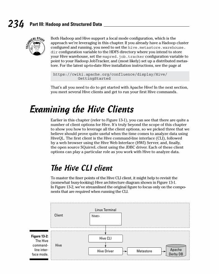
The Hive CLI clientTo master the finer points of the Hive CLI client, it might help to revisit the (somewhat busy-looking) Hive architecture diagram shown in Figure 13-1. In Figure 13-2, we’ve streamlined the original figure to focus only on the compo-nents that are required when running the CLI.
Figure 13-2: The Hive
command-line inter-
face mode.
235 Chapter 13: Applying Structure to Hadoop Data with Hive
Figure 13-2 illustrates the components of Hive that are needed when running the CLI on a Hadoop cluster. In the examples in this chapter, you run Hive in local mode, which uses local storage, rather than the HDFS, for your data.
To run the Hive CLI, you execute the hive command and specify the CLI as the service you want to run. In Listing 13-4, you can see the command that’s required as well as some of our first HiveQL statements. (We have included a steps annotation using the A-B-C model in the listing to direct your attention to the key commands.)
Listing 13-4: Using the Hive CLI to Create a Table
(A) $ $HIVE_HOME/bin hive --service cli(B) hive> set hive.cli.print.current.db=true;(C) hive (default)> CREATE DATABASE ourfirstdatabase;OKTime taken: 3.756 seconds(D) hive (default)> USE ourfirstdatabase;OKTime taken: 0.039 seconds(E) hive (ourfirstdatabase)> CREATE TABLE our_first_table
( > FirstName STRING, > LastName STRING, > EmployeeId INT);OKTime taken: 0.043 secondshive (ourfirstdatabase)> quit;(F) $ ls /home/biadmin/Hive/warehouse/ourfirstdatabase.dbour_first_table
The first command in Listing 13-4 (see Step A) starts the Hive CLI using the $HIVE_HOME environment variable (refer to Listing 13-2). The –service cli command-line option directs the Hive system to start the command-line interface, though you could have chosen other servers. (In fact, you can try a few later in this section.) Next, in Step B, you tell the Hive CLI to print your current working database so that you know where you are in the namespace. (This statement will make sense after we explain how to use the next com-mand, so hold tight.) Continuing in Listing 13-4, in Step C you use HiveQL’s data definition language (DDL) to create your first database. (Remember that databases in Hive are simply namespaces where particular tables reside; because a set of tables can be thought of as a database or schema, you could have used the term SCHEMA in place of DATABASE to accomplish the same result.) More specifically, you’re using DDL to tell the system to create a data-base called ourfirstdatabase and then to make this database the default for subsequent HiveQL DDL commands using the USE command in Step D. In Step E, you create your first table and give it the (quite appropriate) name our_first_table. (Until now, you may have believed that it looks a lot like SQL, with perhaps a few minor differences in syntax depending on which RDBMS you’re accustomed to — and you would have been right.)
236 Part III: Hadoop and Structured Data
The last command, in Step F, carries out a directory listing of your chosen Hive warehouse directory so that you can see that our_first_table has in fact been stored on disk.
You set the hive.metastore.warehouse.dir variable to point to the local directory /home/biadmin/Hive/warehouse in your Linux virtual machine rather than use the HDFS as you would on a proper Hadoop cluster.
After you’ve created a table, it’s interesting to view the table’s metadata. In production environments, you might have dozens of tables or more, so it’s helpful to be able to review the table structure from time to time. You can use a HiveQL command to do this using the Hive CLI, but the Hive Web Interface (HWI) Server provides a helpful interface for this type of operation. (More on HWI in the next section.)
Using the HWI Server instead of the CLI can also be more secure. Careful consideration must be made when using the CLI in production environments because the machine running the CLI must have access to the entire Hadoop cluster. Therefore, system administrators typically put in place tools like the secure shell (ssh) in order to provide controlled and secure access to the machine running the CLI as well as to provide network encryption. However, when the HWI Server is employed, a user can only access Hive data allowed by the HWI Server via his or her web browser
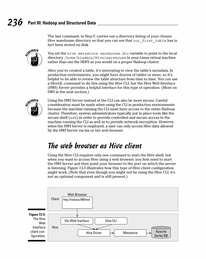
The web browser as Hive clientUsing the Hive CLI requires only one command to start the Hive shell, but when you want to access Hive using a web browser, you first need to start the HWI Server and then point your browser to the port on which the server is listening. Figure 13-3 illustrates how this type of Hive client configuration might work. (Note that even though you might not be using the Hive CLI, it’s not an optional component and is still present.)
Figure 13-3: The Hive
Web Interface
client con-figuration.
237 Chapter 13: Applying Structure to Hadoop Data with Hive
The following steps show you what you need to do before you can start the HWI Server:
1. Using the commands in Listing 13-5 (following this list), configure the $HIVE_HOME/conf/hive-site.xml file to ensure that Hive can find and load the HWI’s Java server pages.
2. The HWI Server requires Apache Ant libraries to run, so you need to download more files. Download Ant from the Apache site at http://ant.apache.org/bindownload.cgi.
3. Install Ant using the following commands:
mkdir antcp apache-ant-1.9.2-bin.tar.gz ant; cd antgunzip apache-ant-1.9.2-bin.tar.gztar xvf apache-ant-1.9.2-bin.tar
4. Set the $ANT_LIB environment variable and start the HWI Server by using the following commands:
$ export ANT_LIB=/home/user/ant/apache-ant-1.9.2/lib$ bin/hive --service hwi13/09/24 16:54:37 INFO hwi.HWIServer: HWI is starting up...13/09/24 16:54:38 INFO mortbay.log: Started
[email protected]:9999
Listing 13-5: Configuring the $HIVE_HOME/conf/hive-site.xml file
<property> <name>hive.hwi.war.file</name> <value>${HIVE_HOME}/lib/hive_hwi.war</value> <description>This is the WAR file with the
jsp content for Hive Web Interface</description> </property>
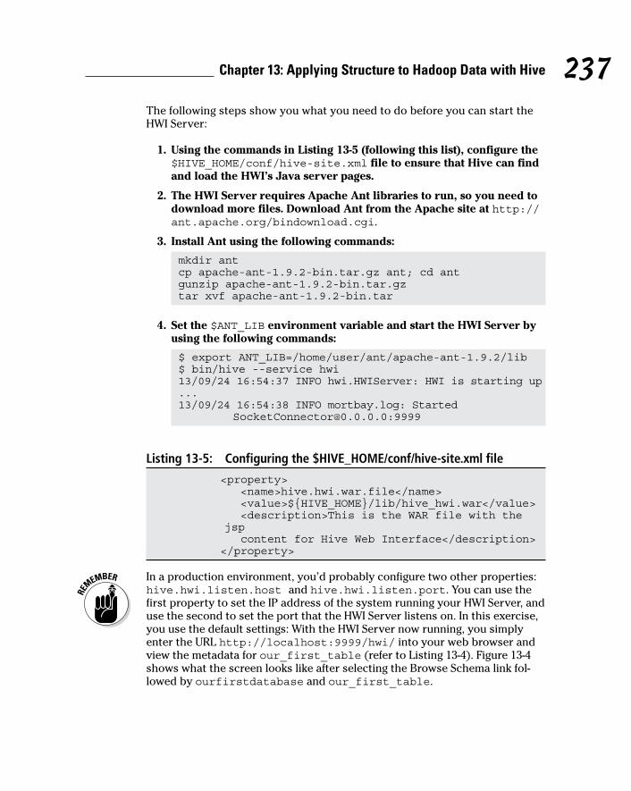
In a production environment, you’d probably configure two other properties: hive.hwi.listen.host and hive.hwi.listen.port. You can use the first property to set the IP address of the system running your HWI Server, and use the second to set the port that the HWI Server listens on. In this exercise, you use the default settings: With the HWI Server now running, you simply enter the URL http://localhost:9999/hwi/ into your web browser and view the metadata for our_first_table (refer to Listing 13-4). Figure 13-4 shows what the screen looks like after selecting the Browse Schema link fol-lowed by ourfirstdatabase and our_first_table.
238 Part III: Hadoop and Structured Data
Figure 13-4: Using the Hive Web
Interface to browse the
metadata.
In production environments, working with the HWI Server can save you the time of loading the Hive distribution on every client — instead, you just point your browser to the server running the HWI. Additionally, you can use the HWI Server to view Hive Thrift Server diagnostics and query tables. The HWI Server allows you to set up batch sessions for long-running queries. To set up a session, you simply click the Create Session link (refer to Figure 13-4).
SQuirreL as Hive client with the JDBC DriverThe last Hive client we discuss and demonstrate in this chapter is the open source tool SQuirreL SQL. You can download this universal SQL client from the SourceForge website: http://sourceforge.net. It provides a user interface to Hive and simplifies the tasks of querying large tables and analyz-ing data with Apache Hive.
Figure 13-5 illustrates how the Hive architecture would work when using tools such as SQuirreL.
In the figure, you can see that the SQuirreL client uses the JDBC APIs to pass commands to the Hive Driver by way of the Server.
For a helpful example of a Hive Java client connecting to the system via the JDBC interface, see
https://cwiki.apache.org/confluence/display/Hive/HiveClient#HiveClient-JDBC
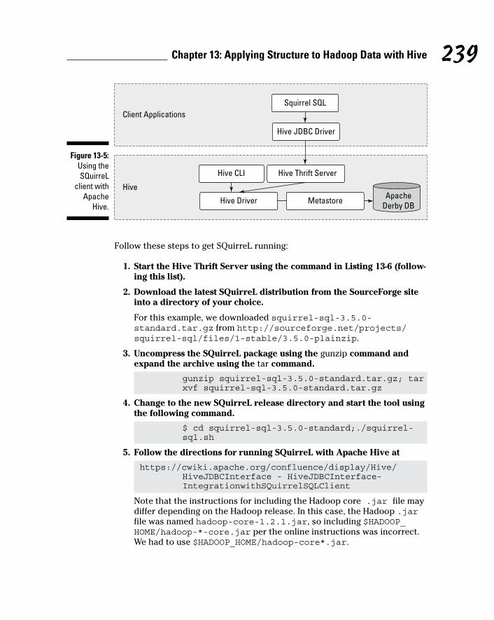
239 Chapter 13: Applying Structure to Hadoop Data with Hive
Figure 13-5: Using the SQuirreL
client with Apache
Hive.
Follow these steps to get SQuirreL running:
1. Start the Hive Thrift Server using the command in Listing 13-6 (follow-ing this list).
2. Download the latest SQuirreL distribution from the SourceForge site into a directory of your choice.
For this example, we downloaded squirrel-sql-3.5.0-standard.tar.gz from http://sourceforge.net/projects/squirrel-sql/files/1-stable/3.5.0-plainzip.
3. Uncompress the SQuirreL package using the gunzip command and expand the archive using the tar command.
gunzip squirrel-sql-3.5.0-standard.tar.gz; tar xvf squirrel-sql-3.5.0-standard.tar.gz
4. Change to the new SQuirreL release directory and start the tool using the following command.
$ cd squirrel-sql-3.5.0-standard;./squirrel-sql.sh
5. Follow the directions for running SQuirreL with Apache Hive at
https://cwiki.apache.org/confluence/display/Hive/HiveJDBCInterface - HiveJDBCInterface-IntegrationwithSQuirrelSQLClient
Note that the instructions for including the Hadoop core .jar file may differ depending on the Hadoop release. In this case, the Hadoop .jar file was named hadoop-core-1.2.1.jar, so including $HADOOP_HOME/hadoop-*-core.jar per the online instructions was incorrect. We had to use $HADOOP_HOME/hadoop-core*.jar.
240 Part III: Hadoop and Structured Data
Listing 13-6: Starting the Hive Thrift Server
$ $HIVE_HOME/bin/hive --service hiveserver -p 10000 -vStarting Hive Thrift ServerStarting Hive Thrift Server on port 10000 with 100 min
worker threads and 2147483647 max worker threads
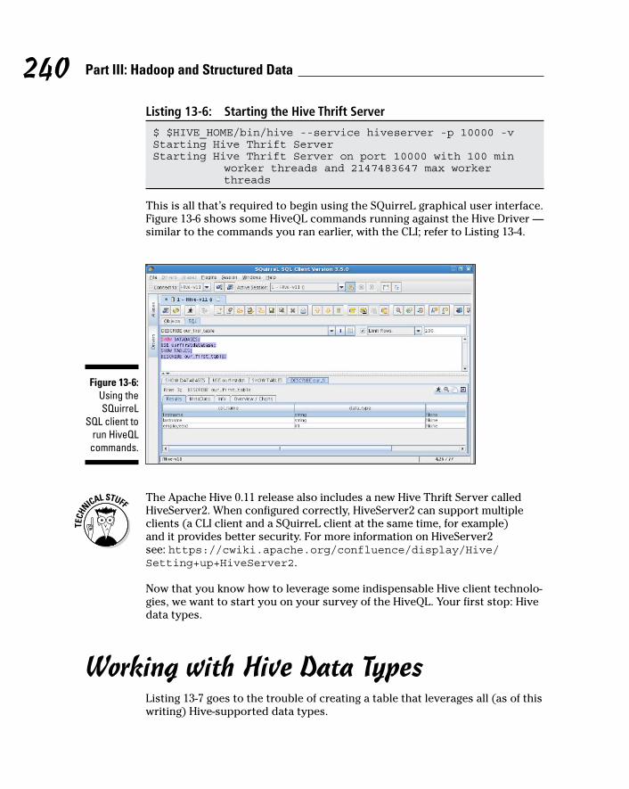
This is all that’s required to begin using the SQuirreL graphical user interface. Figure 13-6 shows some HiveQL commands running against the Hive Driver — similar to the commands you ran earlier, with the CLI; refer to Listing 13-4.
Figure 13-6: Using the SQuirreL
SQL client to run HiveQL
commands.
The Apache Hive 0.11 release also includes a new Hive Thrift Server called HiveServer2. When configured correctly, HiveServer2 can support multiple clients (a CLI client and a SQuirreL client at the same time, for example) and it provides better security. For more information on HiveServer2 see: https://cwiki.apache.org/confluence/display/Hive/Setting+up+HiveServer2.
Now that you know how to leverage some indispensable Hive client technolo-gies, we want to start you on your survey of the HiveQL. Your first stop: Hive data types.
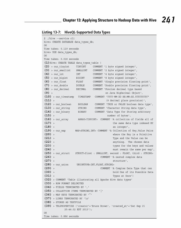
Working with Hive Data TypesListing 13-7 goes to the trouble of creating a table that leverages all (as of this writing) Hive-supported data types.
241 Chapter 13: Applying Structure to Hadoop Data with Hive
Listing 13-7: HiveQL-Supported Data Types
$ ./hive --service clihive> CREATE DATABASE data_types_db;OKTime taken: 0.119 secondshive> USE data_types_db;OKTime taken: 0.018 seconds(1)Hive> CREATE TABLE data_types_table ((2) > our_tinyint TINYINT COMMENT '1 byte signed integer',(3) > our_smallint SMALLINT COMMENT '2 byte signed integer',(4) > our_int INT COMMENT '4 byte signed integer',(5) > our_bigint BIGINT COMMENT '8 byte signed integer',(6) > our_float FLOAT COMMENT 'Single precision floating point',(7) > our_double DOUBLE COMMENT 'Double precision floating point',(8) > our_decimal DECIMAL COMMENT 'Precise decimal type based(9) > on Java BigDecimal Object',(10) > our_timestamp TIMESTAMP COMMENT 'YYYY-MM-DD HH:MM:SS.fffffffff"(11) > (9 decimal place precision)',(12) > our_boolean BOOLEAN COMMENT 'TRUE or FALSE boolean data type',(13) > our_string STRING COMMENT 'Character String data type',(14) > our_binary BINARY COMMENT 'Data Type for Storing arbitrary(15) > number of bytes',(16) > our_array ARRAY<TINYINT> COMMENT 'A collection of fields all of(17) > the same data type indexed BY(18) > an integer',(19) > our_map MAP<STRING,INT> COMMENT 'A Collection of Key,Value Pairs(20) > where the Key is a Primitive(21) > Type and the Value can be(22) > anything. The chosen data(23) > types for the keys and values(24) > must remain the same per map',(25) > our_struct STRUCT<first : SMALLINT, second : FLOAT, third : STRING>(26) > COMMENT 'A nested complex data(27) > structure',(28) > our_union UNIONTYPE<INT,FLOAT,STRING>(29) > COMMENT 'A Complex Data Type that can(30) > hold One of its Possible Data(31) > Types at Once')(32) > COMMENT 'Table illustrating all Apache Hive data types'(33) > ROW FORMAT DELIMITED(34) > FIELDS TERMINATED BY ','(35) > COLLECTION ITEMS TERMINATED BY '|'(36) > MAP KEYS TERMINATED BY '^'(37) > LINES TERMINATED BY '\n'(38) > STORED AS TEXTFILE(39) > TBLPROPERTIES ('creator'='Bruce Brown', 'created_at'='Sat Sep 21
20:46:32 EDT 2013');OKTime taken: 0.886 seconds
242 Part III: Hadoop and Structured Data
We’ve included line numbers with the HiveQL to make it easier to study the table. You can see from the CREATE TABLE statement (refer to Line 1) all the various data types at your disposal (again, as of this writing) in Hive 0.11. One in particular, DECIMAL, is new as of Hive 0.11, so whenever Hive 0.12 is released, check to see whether it has more. (Hint: Watch for the type named DATE.)
Consult the Data Types page in the Apache Hive Language Manual (https://cwiki.apache.org/confluence/display/Hive/LanguageManual+Types) to watch for new data types as the Hive commu-nity continues to develop and create new, innovative features in Hive.
Notice in the table that after every column we created (see Lines 2–31), we wrote a comment (using the HiveQL reserved keyword - COMMENT) giving you information about the Hive data type of the column. Hive supports the Comment feature as a way to document the columns in your tables. Also, Line 32 allows you to add a comment for the entire table. Line 39 starts with the keyword TBLPROPERTIES, which provides a way for you to add metadata to the table. This information can be viewed later, after the table is created, with other HiveQL commands such as DESCRIBE EXTENDED table_name.
Keep in mind that Hive has primitive data types as well as complex data types. The last four columns (see Lines 16–31) in our_datatypes_table are complex data types: ARRAY, MAP, STRUCT, and UNIONTYPE. Their presence provides more proof (if proof is needed) that Hive supports a rich set of data types that enables you to manage diverse data, all under HiveQL.
Finally, Lines 33–38 in the CREATE TABLE statement show off a particularly powerful feature of Hive. Here, the lines let you define the file format when your table gets stored in HDFS and define how fields and rows are delimited. Actually Hive allows you to specify the file format and record format sepa-rately. We discuss this powerful feature of Hive in greater detail in the next section as we tell you more about creating Hive databases and tables.
Creating and Managing Databases and Tables
To fully grasp Hive database and table creation in all its splendor, you need a thorough grounding in what’s referred to as Hive’s data definition language (DDL). You get that grounding in this section, starting with database or schema creation.
243 Chapter 13: Applying Structure to Hadoop Data with Hive
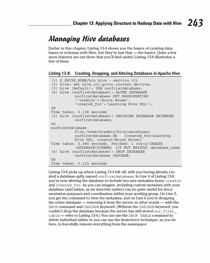
Managing Hive databasesEarlier in this chapter, Listing 13-4 shows you the basics of creating data-bases or schemas with Hive, but they’re just that — the basics. Quite a few more features are out there that you’ll find useful; Listing 13-8 illustrates a few of them.
Listing 13-8: Creating, Dropping, and Altering Databases in Apache Hive
(1) $ $HIVE_HOME/bin hive --service cli(2) hive> set hive.cli.print.current.db=true;(3) hive (default)> USE ourfirstdatabase;(4) hive (ourfirstdatabase)> ALTER DATABASE
ourfirstdatabase SET DBPROPERTIES ('creator'='Bruce Brown', 'created_for'='Learning Hive DDL');
OKTime taken: 0.138 seconds(5) hive (ourfirstdatabase)> DESCRIBE DATABASE EXTENDED
ourfirstdatabase;OKourfirstdatabase
file:/home/biadmin/Hive/warehouse/ourfirstdatabase.db {created_for=Learning Hive DDL, creator=Bruce Brown}
Time taken: 0.084 seconds, Fetched: 1 row(s)CREATE (DATABASE|SCHEMA) [IF NOT EXISTS] database_name
(6) hive (ourfirstdatabase)> DROP DATABASE ourfirstdatabase CASCADE;
OKTime taken: 0.132 seconds
Listing 13-8 picks up where Listing 13-4 left off, with you having already cre-ated a database aptly named ourfirstdatabase. In Line 4 of Listing 13-8, you’re now altering the database to include two new metadata items: creator and created_for. As you can imagine, including custom metadata with your database (and tables, as we describe earlier) can be quite useful for docu-mentation purposes and coordination within your working group. On Line 5, you get the command to view the metadata, and on Line 6 you’re dropping the entire database — removing it from the server, in other words — with the DROP command and CASCADE keyword. (Without the CASCADE keyword, you couldn’t drop the database because the server has still stored our_first_table — refer to Listing 13-4.) You can use the DROP TABLE command to delete individual tables or you can use the brute-force technique, as you do here, to forcefully remove everything from the namespace.
244 Part III: Hadoop and Structured Data
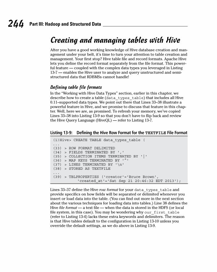
Creating and managing tables with HiveAfter you have a good working knowledge of Hive database creation and man-agement under your belt, it’s time to turn your attention to table creation and management. Your first stop? Hive table file and record formats. Apache Hive lets you define the record format separately from the file format. This power-ful feature — coupled with the complex data types you leveraged in Listing 13-7 — enables the Hive user to analyze and query unstructured and semi-structured data that RDBMSs cannot handle!
Defining table file formatsIn the “Working with Hive Data Types” section, earlier in this chapter, we describe how to create a table (data_types_table) that includes all Hive 0.11–supported data types. We point out there that Lines 33–38 illustrate a powerful feature in Hive, and we promise to discuss that feature in this chap-ter. Well, here we are, as promised. To refresh your memory, we’ve copied Lines 33–38 into Listing 13-9 so that you don’t have to flip back and review the Hive Query Language (HiveQL) — refer to Listing 13-7.
Listing 13-9: Defining the Hive Row Format for the TEXTFILE File Format
(1)Hive> CREATE TABLE data_types_table (...(33) > ROW FORMAT DELIMITED(34) > FIELDS TERMINATED BY ','(35) > COLLECTION ITEMS TERMINATED BY '|'(36) > MAP KEYS TERMINATED BY '^'(37) > LINES TERMINATED BY '\n'(38) > STORED AS TEXTFILE...(39) > TBLPROPERTIES ('creator'='Bruce Brown',
'created_at'='Sat Sep 21 20:46:32 EDT 2013');
Lines 33–37 define the Hive row format for your data_types_table and provide specifics on how fields will be separated or delimited whenever you insert or load data into the table. (You can find out more in the next section about the various techniques for loading data into tables.) Line 38 defines the Hive file format — a text file — when the data is stored in the HDFS (or local file system, in this case). You may be wondering why our_first_table (refer to Listing 13-4) lacks these extra keywords and delimiters. The reason is that Hive tables default to the configuration in Listing 13-10 unless you override the default settings, as we do above in Listing 13-9.
245 Chapter 13: Applying Structure to Hadoop Data with Hive
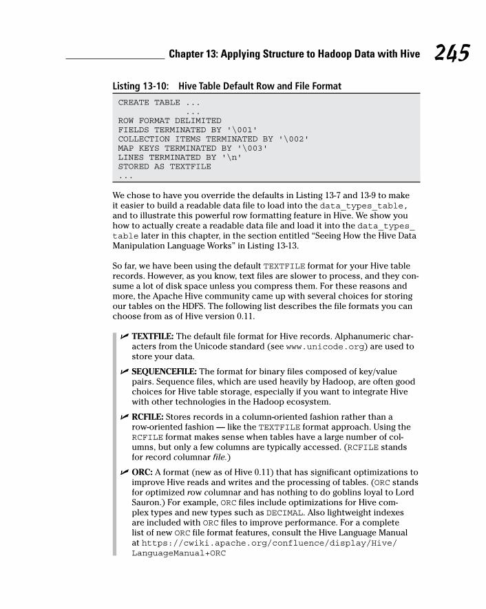
Listing 13-10: Hive Table Default Row and File Format
CREATE TABLE ... ...ROW FORMAT DELIMITEDFIELDS TERMINATED BY '\001'COLLECTION ITEMS TERMINATED BY '\002'MAP KEYS TERMINATED BY '\003'LINES TERMINATED BY '\n'STORED AS TEXTFILE...
We chose to have you override the defaults in Listing 13-7 and 13-9 to make it easier to build a readable data file to load into the data_types_table, and to illustrate this powerful row formatting feature in Hive. We show you how to actually create a readable data file and load it into the data_types_table later in this chapter, in the section entitled “Seeing How the Hive Data Manipulation Language Works” in Listing 13-13.
So far, we have been using the default TEXTFILE format for your Hive table records. However, as you know, text files are slower to process, and they con-sume a lot of disk space unless you compress them. For these reasons and more, the Apache Hive community came up with several choices for storing our tables on the HDFS. The following list describes the file formats you can choose from as of Hive version 0.11.
✓ TEXTFILE: The default file format for Hive records. Alphanumeric char-acters from the Unicode standard (see www.unicode.org) are used to store your data.
✓ SEQUENCEFILE: The format for binary files composed of key/value pairs. Sequence files, which are used heavily by Hadoop, are often good choices for Hive table storage, especially if you want to integrate Hive with other technologies in the Hadoop ecosystem.
✓ RCFILE: Stores records in a column-oriented fashion rather than a row-oriented fashion — like the TEXTFILE format approach. Using the RCFILE format makes sense when tables have a large number of col-umns, but only a few columns are typically accessed. (RCFILE stands for record columnar file.)
✓ ORC: A format (new as of Hive 0.11) that has significant optimizations to improve Hive reads and writes and the processing of tables. (ORC stands for optimized row columnar and has nothing to do goblins loyal to Lord Sauron.) For example, ORC files include optimizations for Hive com-plex types and new types such as DECIMAL. Also lightweight indexes are included with ORC files to improve performance. For a complete list of new ORC file format features, consult the Hive Language Manual at https://cwiki.apache.org/confluence/display/Hive/LanguageManual+ORC
246 Part III: Hadoop and Structured Data
✓ INPUTFORMAT, OUTPUTFORMAT: Lets you specify the Java class that will read data from the Hive table. OUTPUTFORMAT does the same thing for writing data to the Hive table. The keywords in the earlier table entries (TEXTFILE, for example) provide shortened syntax so that you don’t have to specify both INPUTFORMAT and OUTPUTFORMAT for every CREATE TABLE statement. Of course, it enables customization and can be quite pow-erful under the right circumstances. To see the default settings for the table, simply execute a DESCRIBE EXTENDED tablename HiveQL statement and you’ll see the INPUTFORMAT and OUTPUTFORMAT classes for your table.
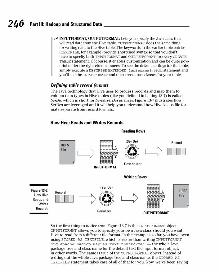
Defining table record formatsThe Java technology that Hive uses to process records and map them to column data types in Hive tables (like you defined in Listing 13-7) is called SerDe, which is short for SerializerDeserializer. Figure 13-7 illustrates how SerDes are leveraged and it will help you understand how Hive keeps file for-mats separate from record formats.
Figure 13-7: How Hive
Reads and Writes
Records
So the first thing to notice from Figure 13-7 is the INPUTFORMAT object. INPUTFORMAT allows you to specify your own Java class should you want Hive to read from a different file format. In the examples so far, you have been using STORED AS TEXTFILE, which is easier than writing INPUTFORMAT org.apache.hadoop.mapred.TextInputFormat — the whole Java package tree and class name for the default text file input format object, in other words. The same is true of the OUTPUTFORMAT object. Instead of writing out the whole Java package tree and class name, the STORED AS TEXTFILE statement takes care of all of that for you. Now, we’ve been saying
247 Chapter 13: Applying Structure to Hadoop Data with Hive
that Hive allows you to separate your record format from your file format so how exactly do you accomplish this? Simple, you either replace STORED AS TEXTFILE with something like STORED AS RCFILE, or you can create your own Java class and specify the input and output classes using INPUTFORMAT packagepath.classname and OUTPUTFORMAT packagepath.classname.
Finally notice that when Hive is reading data from the HDFS (or local file system), a Java Deserializer formats the data into a record that maps to table column data types. This would characterize the data flow for a HiveQL SELECT statement which you’ll be able to try out in “Querying and analyzing data” section below. When Hive is writing data, a Java Serializer accepts the record Hive uses and translates it such that the OUTPUTFORMAT class can write it to the HDFS (or local file system). This would characterize the data flow for a HiveQL CREATE-TABLE-AS-SELECT statement which you’ll be able to try out in “Mastering the Hive data-manipulation language” section below. So the INPUTFORMAT, OUTPUTFORMAT and SerDe objects allow Hive to separate the table record format from the table file format. You’ll be able to see this in action in two examples below but first we want to expose you to some SerDe options.
Hive bundles a number of SerDes for you to choose from, and you’ll find a larger number available from third parties if you search online. You can also develop your own SerDes if you have a more unusual data type that you want to manage with a Hive table. (Possible examples here are video data and e-mail data.) In the list below, we describe some of the SerDes provided with Hive as well as one third-party option that you may find useful.
✓ LazySimpleSerDe: The default SerDe that’s used with the TEXTFILE format; it would be used with our_first_table from Listing 13-4 and with data_types_table from Listing 13-7.
✓ ColumnarSerDe: Used with the RCFILE format.
✓ RegexSerDe: The regular expression SerDe, which ships with Hive to enable the parsing of text files, RegexSerDe can form a powerful approach for building structured data in Hive tables from unstructured blogs, semi-structured log files, e-mails, tweets, and other data from social media. Regular expressions allow you to extract meaningful infor-mation (an e-mail address, for example) with HiveQL from an unstruc-tured or semi-structured text document incompatible with traditional SQL and RDBMSs.
✓ HBaseSerDe: Included with Hive to enables it to integrate with HBase. You can store Hive tables in HBase by leveraging this SerDe.
✓ JSONSerDe: A third-party SerDe for reading and writing JSON data records with Hive. We quickly found (via Google and GitHub) two JSON SerDes by searching online for the phrase json serde for hive.
✓ AvroSerDe: Included with Hive so that you can read and write Avro data in Hive tables.
248 Part III: Hadoop and Structured Data
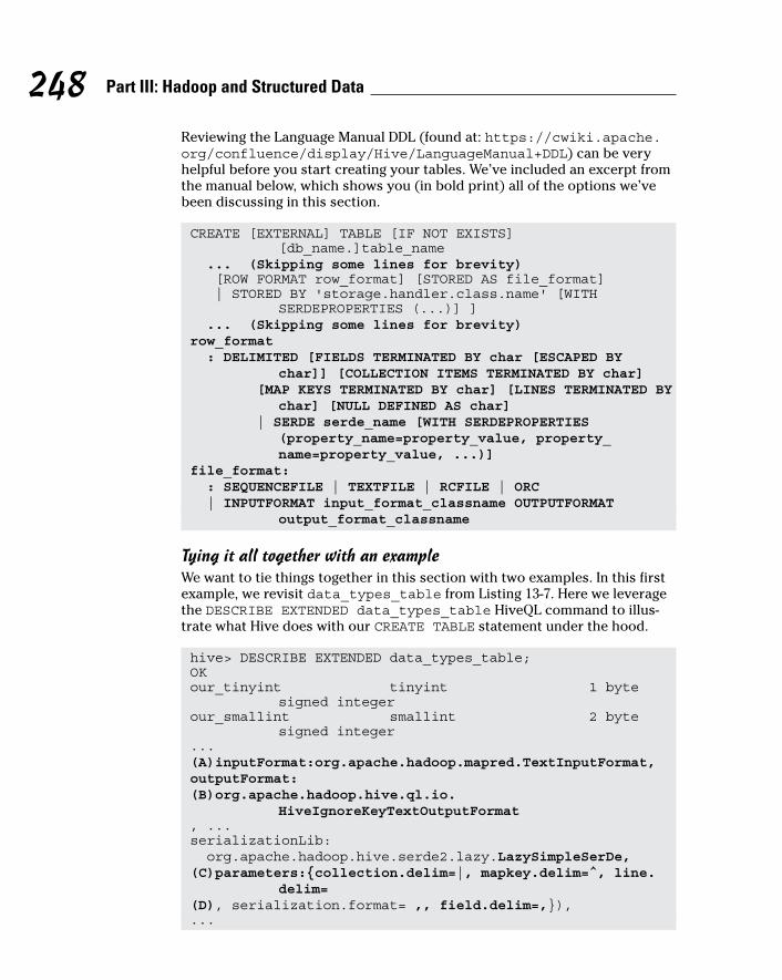
Reviewing the Language Manual DDL (found at: https://cwiki.apache.org/confluence/display/Hive/LanguageManual+DDL) can be very helpful before you start creating your tables. We’ve included an excerpt from the manual below, which shows you (in bold print) all of the options we’ve been discussing in this section.
CREATE [EXTERNAL] TABLE [IF NOT EXISTS] [db_name.]table_name
... (Skipping some lines for brevity) [ROW FORMAT row_format] [STORED AS file_format] | STORED BY 'storage.handler.class.name' [WITH
SERDEPROPERTIES (...)] ] ... (Skipping some lines for brevity) row_format : DELIMITED [FIELDS TERMINATED BY char [ESCAPED BY
char]] [COLLECTION ITEMS TERMINATED BY char] [MAP KEYS TERMINATED BY char] [LINES TERMINATED BY
char] [NULL DEFINED AS char] | SERDE serde_name [WITH SERDEPROPERTIES
(property_name=property_value, property_name=property_value, ...)]
file_format: : SEQUENCEFILE | TEXTFILE | RCFILE | ORC | INPUTFORMAT input_format_classname OUTPUTFORMAT
output_format_classname
Tying it all together with an exampleWe want to tie things together in this section with two examples. In this first example, we revisit data_types_table from Listing 13-7. Here we leverage the DESCRIBE EXTENDED data_types_table HiveQL command to illus-trate what Hive does with our CREATE TABLE statement under the hood.
hive> DESCRIBE EXTENDED data_types_table;OKour_tinyint tinyint 1 byte
signed integerour_smallint smallint 2 byte
signed integer...(A)inputFormat:org.apache.hadoop.mapred.TextInputFormat,outputFormat:(B)org.apache.hadoop.hive.ql.io.
HiveIgnoreKeyTextOutputFormat, ...serializationLib: org.apache.hadoop.hive.serde2.lazy.LazySimpleSerDe, (C)parameters:{collection.delim=|, mapkey.delim=^, line.
delim=(D), serialization.format= ,, field.delim=,}), ...
249 Chapter 13: Applying Structure to Hadoop Data with Hive
Notice that Hive provides an INPUTFORMAT and OUTPUTFORMAT class for you when you specify STORED AS TEXTFILE, as we did in line 38 from Listing 13-7. Also note how Hive included the default LazySimpleSerDe. The row format delim-iters that you specified in lines 33 through 37 from Listing 13-7 are inserted as parameters to the LazySimpleSerDe so the records in the text file can be parsed and translated into column types by the SerDe or written in proper format to the text file.
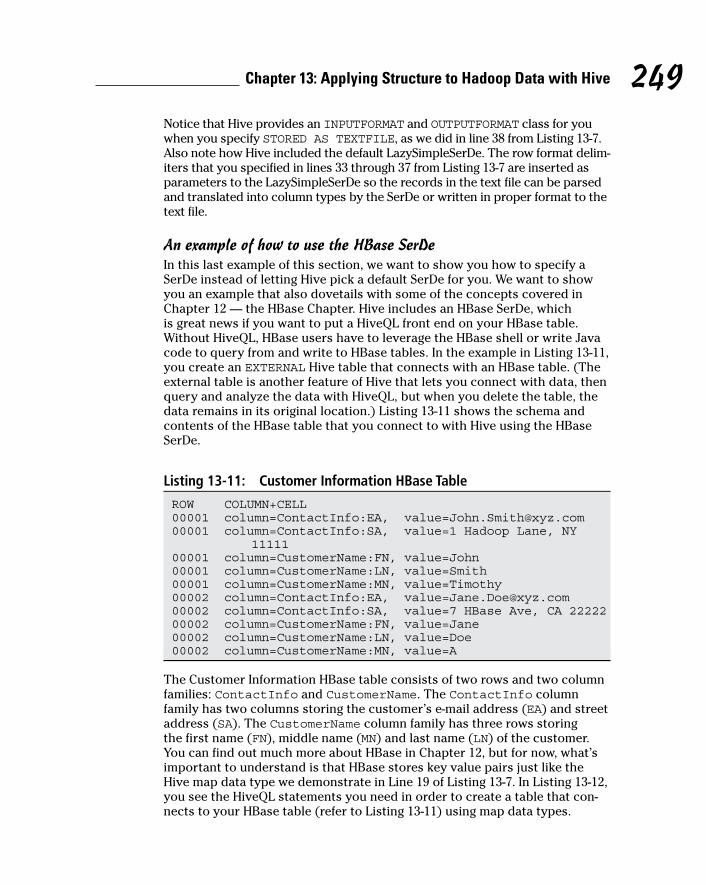
An example of how to use the HBase SerDeIn this last example of this section, we want to show you how to specify a SerDe instead of letting Hive pick a default SerDe for you. We want to show you an example that also dovetails with some of the concepts covered in Chapter 12 — the HBase Chapter. Hive includes an HBase SerDe, which is great news if you want to put a HiveQL front end on your HBase table. Without HiveQL, HBase users have to leverage the HBase shell or write Java code to query from and write to HBase tables. In the example in Listing 13-11, you create an EXTERNAL Hive table that connects with an HBase table. (The external table is another feature of Hive that lets you connect with data, then query and analyze the data with HiveQL, but when you delete the table, the data remains in its original location.) Listing 13-11 shows the schema and contents of the HBase table that you connect to with Hive using the HBase SerDe.
Listing 13-11: Customer Information HBase Table
ROW COLUMN+CELL00001 column=ContactInfo:EA, [email protected] column=ContactInfo:SA, value=1 Hadoop Lane, NY
1111100001 column=CustomerName:FN, value=John00001 column=CustomerName:LN, value=Smith00001 column=CustomerName:MN, value=Timothy00002 column=ContactInfo:EA, [email protected] column=ContactInfo:SA, value=7 HBase Ave, CA 2222200002 column=CustomerName:FN, value=Jane00002 column=CustomerName:LN, value=Doe00002 column=CustomerName:MN, value=A
The Customer Information HBase table consists of two rows and two column families: ContactInfo and CustomerName. The ContactInfo column family has two columns storing the customer’s e-mail address (EA) and street address (SA). The CustomerName column family has three rows storing the first name (FN), middle name (MN) and last name (LN) of the customer. You can find out much more about HBase in Chapter 12, but for now, what’s important to understand is that HBase stores key value pairs just like the Hive map data type we demonstrate in Line 19 of Listing 13-7. In Listing 13-12, you see the HiveQL statements you need in order to create a table that con-nects to your HBase table (refer to Listing 13-11) using map data types.
250 Part III: Hadoop and Structured Data
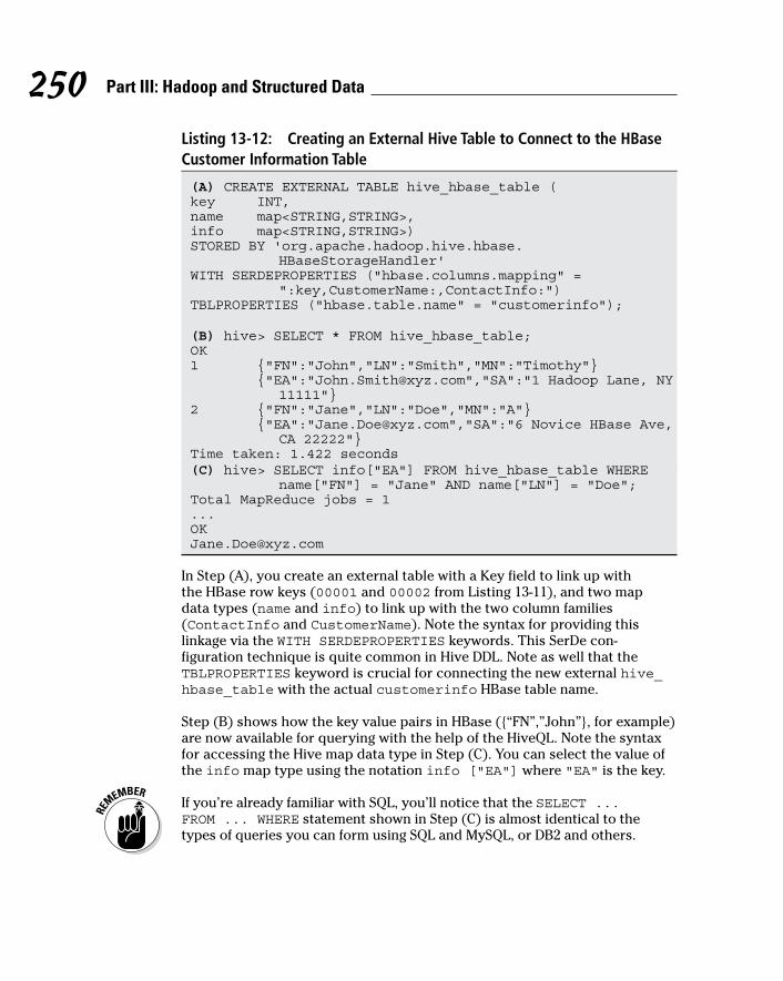
Listing 13-12: Creating an External Hive Table to Connect to the HBase Customer Information Table
(A) CREATE EXTERNAL TABLE hive_hbase_table (key INT,name map<STRING,STRING>,info map<STRING,STRING>)STORED BY 'org.apache.hadoop.hive.hbase.
HBaseStorageHandler'WITH SERDEPROPERTIES ("hbase.columns.mapping" =
":key,CustomerName:,ContactInfo:")TBLPROPERTIES ("hbase.table.name" = "customerinfo"); (B) hive> SELECT * FROM hive_hbase_table;OK1 {"FN":"John","LN":"Smith","MN":"Timothy"} {"EA":"[email protected]","SA":"1 Hadoop Lane, NY
11111"}2 {"FN":"Jane","LN":"Doe","MN":"A"} {"EA":"[email protected]","SA":"6 Novice HBase Ave,
CA 22222"}Time taken: 1.422 seconds(C) hive> SELECT info["EA"] FROM hive_hbase_table WHERE
name["FN"] = "Jane" AND name["LN"] = "Doe";Total MapReduce jobs = [email protected]
In Step (A), you create an external table with a Key field to link up with the HBase row keys (00001 and 00002 from Listing 13-11), and two map data types (name and info) to link up with the two column families (ContactInfo and CustomerName). Note the syntax for providing this linkage via the WITH SERDEPROPERTIES keywords. This SerDe con-figuration technique is quite common in Hive DDL. Note as well that the TBLPROPERTIES keyword is crucial for connecting the new external hive_hbase_table with the actual customerinfo HBase table name.
Step (B) shows how the key value pairs in HBase ({“FN”,”John”}, for example) are now available for querying with the help of the HiveQL. Note the syntax for accessing the Hive map data type in Step (C). You can select the value of the info map type using the notation info ["EA"] where "EA" is the key.
If you’re already familiar with SQL, you’ll notice that the SELECT ... FROM ... WHERE statement shown in Step (C) is almost identical to the types of queries you can form using SQL and MySQL, or DB2 and others.
251 Chapter 13: Applying Structure to Hadoop Data with Hive
Seeing How the Hive Data Manipulation Language Works
In the first half of this chapter, we walk you through a couple of CREATE TABLE examples using the Hive CLI (refer to Listings 13-4 and 13-7), and you can see how Hive allows you to control your table’s file and record stor-age formats. Now it’s time to delve into Hive’s data manipulation language (DML) — it lets you load and insert data into tables and create tables from other tables. We even go all out and provide examples that illustrate four ways to input data into Hive tables.
LOAD DATA examplesWe have you start out by placing data into the data_types_table you cre-ated using Listing 13-7. Doing so illustrates the LOAD DATA command and will serve to cement some of the concepts from the last section. The syntax for the LOAD DATA command is shown in Listing 13-13.
Listing 13-13: LOAD DATA Command Syntax
"LOAD DATA [LOCAL] INPATH 'path to file' [OVERWRITE] INTO TABLE 'table name' [PARTITION partition column1 = value1, partition column2 = value2,...]
A few areas in Listing 13-13 need an explanation. First, the optional LOCAL keyword tells Hive to copy data from the input file on the local file system into the Hive data warehouse directory (in our case, on the local file system). Without the LOCAL keyword, the data is simply moved (not copied) into the warehouse directory. Also you should be aware that when running in distrib-uted mode, if you omit the LOCAL keyword Hive assumes your data is already in the HDFS, and in this case moves the data from its current HDFS location into the HDFS warehouse directory. Second, the optional OVERWRITE key-word, as you might imagine, causes the system to overwrite data in the speci-fied table if it already has data stored in it. Finally, the optional PARTITION list tells Hive to partition the storage of the table into different directories in the data warehouse directory structure. This powerful concept improves query performance in Hive, and we demonstrate its use later in this section. When you think about the magnitude of data that can be managed by Hive in the HDFS, partitioning makes a lot of sense. Rather than run a MapReduce job over the entire table to find the data you want to view or analyze, you can isolate a segment of the table and save a lot of system time with partitions.
Apache Hive uses the MapReduce technology within Hadoop to query and analyze tables — though, in some cases, MapReduce is not used. It turns out that you can set the configuration variable hive.exec.mode.local.auto
252 Part III: Hadoop and Structured Data
in the hive-site.xml file. When the variable is set to true, Hive tries to execute queries on small data sets locally without MapReduce whenever pos-sible, to speed execution.
Listing 13-14 shows the commands to use to load the data_types_table with data. Again, we’ve annotated the listing so that we can discuss each step.
Listing 13-14: Loading our_first_table with Data
(A) $ cat data.txt100,32000,2000000,9200000000000000000,0.15625,4.9406564584
124654,1.23E+3,2013-09-21 20:19:52.025,true,test string,\0xFFFFDDDDEEEEAAAA,1|2|3|4,key^1024,1|3.1459|test struct,2|test union(B) hive (data_types_db)> LOAD DATA LOCAL INPATH
'/home/biadmin/Hive/data.txt' INTO TABLE data_types_table;
Copying data from file:/home/biadmin/Hive/data.txtCopying file: file:/home/biadmin/Hive/data.txtLoading data to table data_types_db.data_types_tableTable data_types_db.data_types_table stats:
[num_partitions: 0, num_files: 1, num_rows: 0, total_size: 185, raw_data_size: 0]
OKTime taken: 0.287 seconds(C) hive> SELECT * FROM data_types_table;OK100 32000 2000000 9200000000000000000 0.15625
4.9406564584124651230 2013-09-21 20:19:52.025 true test string\0xFFFFDDDDEEEEAAAA [1,2,3,4] {"key":1024}{"first":1,"second":3.1459,"third":"test struct"}(D) {2:"test union"}Time taken: 0.201 seconds, Fetched: 1 row(s)
Step (A) is a listing (using the Unix cat command) of data you intend to load. This data file has only one record in it, but there’s a value for each field in the table. Note the field and complex type delimiters. As we specified at table cre-ation time (refer to Listing 13-7 or 13-9), fields are separated by a comma; col-lections (such as STRUCT and UNIONTYPE) are separated by the vertical bar or pipe character (|̄); and the MAP keys and values are separated by the caret character (^̄). Step (B) has the LOAD DATA command, and in Step (C) you’re retrieving the record you just loaded in Step (B) so that you can view the data.
The data retrieved using the SELECT command is as expected, but the last field — see line (D) — needs some attention. Note how the UNIONTYPE works. UNIONTYPEs in Hive can store different data types, but only one at a time. In the data.txt file you list in Step (A), you specify to use the third data type in the our_union field. (It’s the third one because you start counting at zero, of course.) So you specify a string — in this case, test union — after the 2 in the data file.
253 Chapter 13: Applying Structure to Hadoop Data with Hive
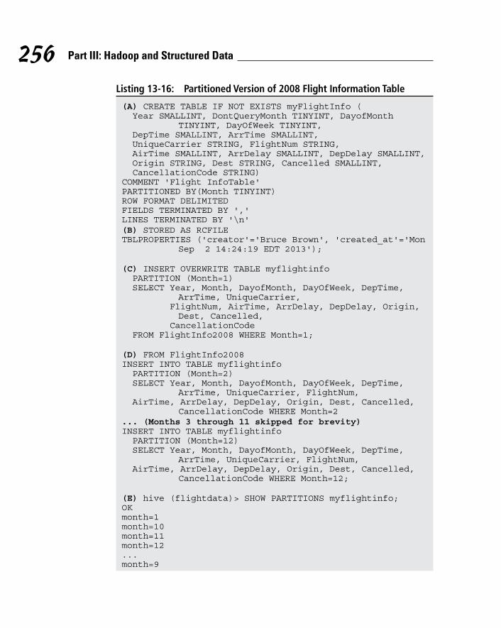
The last example in this subsection sets up other examples later in this chapter. We have downloaded some historical airline flight data for the years 2007 and 2008 from the website http://stat-computing.org/dataexpo/2009/the-data.html. This data was compiled by the Research and Innovative Technology Administration, which coordinates with the U.S. Department of Transportation’s Bureau of Transportation Statistics to pro-vide data to statisticians and scientists. It’s a classic use case for Apache Hive: We show you how to load this airline data into a Hive table, and then you get a chance to perform some analysis with HiveQL!
To put this airline data in perspective, the data for the year 2007 is approxi-mately 671MB and the data for the year 2008 is 659MB. We don’t want to over-load the disk space on your virtual machine, so we downloaded only a few data files, though it appears that the files range between 100MB and 659MB in the case of the year 2008. If you were to download all 22 years’ worth of data from http://stat-computing.org/dataexpo/2009/the-data.html, it would amount to well over 1 terabyte (TB) of information. This is a typical big data use case for Apache Hadoop and Hive running on a cluster of Linux servers. If you would attempt to analyze that much data on classic relational database systems, it would be costly and cumbersome at best.
So, after downloading the data and studying the data types listed on the website, we created two identical tables, named FlightInfo2007 and FlightInfo2008, as you can see in steps (A) and (F) in Listing 13-15. Note that this data is posted on the aforementioned website as comma-separated text, so you’ll use the classic text file format for your records, and we’ve specified comma separation for the record fields. Hive’s LazySimpleSerDe does the rest of the job for you. Step (B) should also look familiar except that we didn’t use the LOCAL keyword. That’s because these files are large; you’ll move the data into your Hive warehouse, not make another copy on your small and tired laptop disk. You’d likely want to do the same thing on a real cluster and not waste the storage.
Listing 13-15: Flight Information Tables from 2007 and 2008
(A) CREATE TABLE IF NOT EXISTS FlightInfo2007 ( Year SMALLINT, Month TINYINT, DayofMonth TINYINT,
DayOfWeek TINYINT, DepTime SMALLINT, CRSDepTime SMALLINT, ArrTime SMALLINT,
CRSArrTime SMALLINT, UniqueCarrier STRING, FlightNum STRING, TailNum STRING, ActualElapsedTime SMALLINT, CRSElapsedTime SMALLINT, AirTime SMALLINT, ArrDelay SMALLINT, DepDelay SMALLINT, Origin STRING, Dest STRING,Distance INT, TaxiIn SMALLINT, TaxiOut SMALLINT, Cancelled SMALLINT, CancellationCode STRING, Diverted SMALLINT, CarrierDelay SMALLINT, WeatherDelay SMALLINT, NASDelay SMALLINT, SecurityDelay SMALLINT,
LateAircraftDelay SMALLINT)COMMENT 'Flight InfoTable'
(continued)
254 Part III: Hadoop and Structured Data
ROW FORMAT DELIMITEDFIELDS TERMINATED BY ','LINES TERMINATED BY '\n'STORED AS TEXTFILETBLPROPERTIES ('creator'='Bruce Brown', 'created_at'='Thu
Sep 19 10:58:00 EDT 2013'); (B) hive (flightdata)> LOAD DATA INPATH '/home/biadmin/
Hive/Data/2007.csv' INTO TABLE FlightInfo2007;Loading data to table flightdata.flightinfo2007Table flightdata.flightinfo2007 stats: [num_partitions:
0, num_files: 2, num_rows: 0, total_size: 1405756086, raw_data_size: 0]
OKTime taken: 0.284 seconds;(C) hive (flightdata)> SELECT * FROM FlightInfo2007 LIMIT
2;OKNULL NULL NULL NULL NULL NULL NULL
NULL UniqueCarrier FlightNum TailNum NULL NULLNULL NULL NULL Origin Dest NULL NULL NULL NULL CancellationCode NULL NULL NULLNULL NULL NULL
2007 1 1 1 1232 1225 1341 1340 WN 2891 N351 69 75 54 1 7SMF ONT 389 4 11 0 0 0 0 0 0 0
Time taken: 0.087 seconds, Fetched: 2 row(s) (D) LOAD DATA INPATH '/home/biadmin/Hive/Data/2007.csv'
OVERWRITE INTO TABLE FlightInfo2007;(E) hive (flightdata)> SELECT * FROM FlightInfo2007 LIMIT
2;OK2007 1 1 1 1232 1225 1341
1340 WN 2891 N351 69 75 54 1 7SMF ONT 389 4 11 0 0 0 0 0 0 0
2007 1 1 1 1918 1905 2043 2035 WN 462 N370 85 90 74 8 13 SMF PDX 479 5 6 0 0 0 0 0 0 0
Time taken: 0.089 seconds, Fetched: 2 row(s) (F) CREATE TABLE IF NOT EXISTS FlightInfo2008 LIKE
FlightInfo2007;(G) LOAD DATA INPATH '/home/biadmin/Hive/Data/2008.csv'
INTO TABLE FlightInfo2008;
Listing 13-15 (continued)
255 Chapter 13: Applying Structure to Hadoop Data with Hive
To test the LOAD DATA command and make sure everything works, you use the SELECT command as shown in the previous example, but this time you also use the LIMIT keyword [see step (C)] because this table is huge. Note that initially you have a bit of problem with the FlightInfo2007 table. Why are you seeing mostly all NULL values in the first record? The answer is that the 2007.csv file has a header on the first line giving the descriptions of the columns in the rest of the file. These descriptions match the website’s explanation of the fields we used to define the data types. So the solution was simple: We downloaded another copy of the data, deleted the header line, and ran the command again — this time, using the OVERWRITE keyword. Now, in Step (E) you can see that the problem has been solved. In Step (F), the LIKE keyword instructs Hive to copy the existing FlightInfo2007 table definition when creating the FlightInfo2008 table. In Step (G) you’re using the same technique as in Step (B).
The problem with NULL values seemed trivial enough, but this example points to an interesting aspect of Hive that we need to explain before we move on to the next Hive DML command.
In Listing 13-15, Hive could not (at first) match the first record with the data types you specified in your CREATE TABLE statement. So the system showed NULL values in place of the real data, and the command completed success-fully. This behavior illustrates that Hive uses a Schema on Read verification approach as opposed to the Schema on Write verification approach, which you find in RDBMS technologies. This is one reason why Hive is so powerful for big data analytics — it lets you discover and explore your data in a relaxed fashion as opposed to a strict structured approach. A typical RDBMS system would have returned errors when the data didn’t match. Hive didn’t return an error when we tried to load data into the table that didn’t match our schema — it simply showed NULL values, and then you figured out the bit about the data-types disconnect by inspecting the data and adjusted accordingly.
INSERT examplesAnother Hive DML command to explore is the INSERT command. You basi-cally have three INSERT variants; we show you two of them in Listing 13-16. To demonstrate this new DML command, we have you create a new table that will hold a subset of the data in the FlightInfo2008 table you created in the previous example. In Step (A), you create this new table and specify that the file format will be row columnar (Step (B)) instead of text. This format is more compact than text and often performs better, depending on your access patterns. (If you’re accessing a small subset of columns instead of entire rows, try the RCFILE format.)
The default SerDe for RCFILE format is the ColumnarSerDe. You can verify this fact by running the DESCRIBE EXTENDED myFlightInfo HiveQL com-mand from the command line interface.
256 Part III: Hadoop and Structured Data
Listing 13-16: Partitioned Version of 2008 Flight Information Table
(A) CREATE TABLE IF NOT EXISTS myFlightInfo ( Year SMALLINT, DontQueryMonth TINYINT, DayofMonth
TINYINT, DayOfWeek TINYINT, DepTime SMALLINT, ArrTime SMALLINT, UniqueCarrier STRING, FlightNum STRING, AirTime SMALLINT, ArrDelay SMALLINT, DepDelay SMALLINT, Origin STRING, Dest STRING, Cancelled SMALLINT, CancellationCode STRING)COMMENT 'Flight InfoTable'PARTITIONED BY(Month TINYINT)ROW FORMAT DELIMITEDFIELDS TERMINATED BY ','LINES TERMINATED BY '\n'(B) STORED AS RCFILETBLPROPERTIES ('creator'='Bruce Brown', 'created_at'='Mon
Sep 2 14:24:19 EDT 2013'); (C) INSERT OVERWRITE TABLE myflightinfo PARTITION (Month=1) SELECT Year, Month, DayofMonth, DayOfWeek, DepTime,
ArrTime, UniqueCarrier, FlightNum, AirTime, ArrDelay, DepDelay, Origin,
Dest, Cancelled, CancellationCode FROM FlightInfo2008 WHERE Month=1; (D) FROM FlightInfo2008INSERT INTO TABLE myflightinfo PARTITION (Month=2) SELECT Year, Month, DayofMonth, DayOfWeek, DepTime,
ArrTime, UniqueCarrier, FlightNum, AirTime, ArrDelay, DepDelay, Origin, Dest, Cancelled,
CancellationCode WHERE Month=2... (Months 3 through 11 skipped for brevity)INSERT INTO TABLE myflightinfo PARTITION (Month=12) SELECT Year, Month, DayofMonth, DayOfWeek, DepTime,
ArrTime, UniqueCarrier, FlightNum, AirTime, ArrDelay, DepDelay, Origin, Dest, Cancelled,
CancellationCode WHERE Month=12; (E) hive (flightdata)> SHOW PARTITIONS myflightinfo;OKmonth=1month=10month=11month=12...month=9
257 Chapter 13: Applying Structure to Hadoop Data with Hive
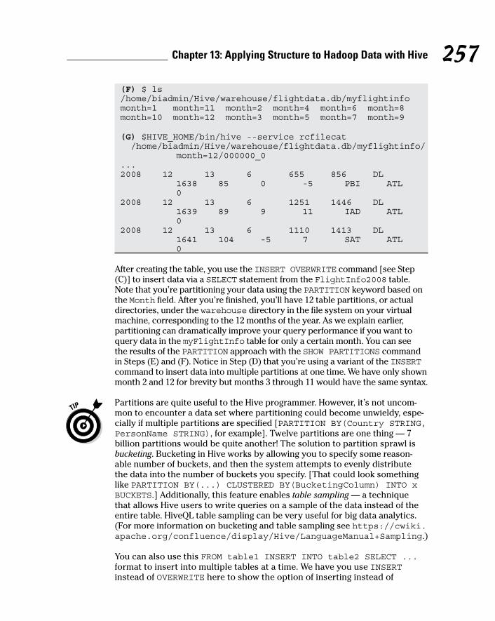
(F) $ ls /home/biadmin/Hive/warehouse/flightdata.db/myflightinfomonth=1 month=11 month=2 month=4 month=6 month=8month=10 month=12 month=3 month=5 month=7 month=9 (G) $HIVE_HOME/bin/hive --service rcfilecat /home/biadmin/Hive/warehouse/flightdata.db/myflightinfo/
month=12/000000_0...2008 12 13 6 655 856 DL
1638 85 0 -5 PBI ATL 0
2008 12 13 6 1251 1446 DL 1639 89 9 11 IAD ATL 0
2008 12 13 6 1110 1413 DL 1641 104 -5 7 SAT ATL 0
After creating the table, you use the INSERT OVERWRITE command [see Step (C)] to insert data via a SELECT statement from the FlightInfo2008 table. Note that you’re partitioning your data using the PARTITION keyword based on the Month field. After you’re finished, you’ll have 12 table partitions, or actual directories, under the warehouse directory in the file system on your virtual machine, corresponding to the 12 months of the year. As we explain earlier, partitioning can dramatically improve your query performance if you want to query data in the myFlightInfo table for only a certain month. You can see the results of the PARTITION approach with the SHOW PARTITIONS command in Steps (E) and (F). Notice in Step (D) that you’re using a variant of the INSERT command to insert data into multiple partitions at one time. We have only shown month 2 and 12 for brevity but months 3 through 11 would have the same syntax.
Partitions are quite useful to the Hive programmer. However, it’s not uncom-mon to encounter a data set where partitioning could become unwieldy, espe-cially if multiple partitions are specified [PARTITION BY(Country STRING, PersonName STRING), for example]. Twelve partitions are one thing — 7 billion partitions would be quite another! The solution to partition sprawl is bucketing. Bucketing in Hive works by allowing you to specify some reason-able number of buckets, and then the system attempts to evenly distribute the data into the number of buckets you specify. [That could look something like PARTITION BY(...) CLUSTERED BY(BucketingColumn) INTO x BUCKETS.] Additionally, this feature enables table sampling — a technique that allows Hive users to write queries on a sample of the data instead of the entire table. HiveQL table sampling can be very useful for big data analytics. (For more information on bucketing and table sampling see https://cwiki.apache.org/confluence/display/Hive/LanguageManual+Sampling.)
You can also use this FROM table1 INSERT INTO table2 SELECT ... format to insert into multiple tables at a time. We have you use INSERT instead of OVERWRITE here to show the option of inserting instead of
258 Part III: Hadoop and Structured Data
overwriting. Hive allows only appends, not inserts, into tables, so the INSERT keyword simply instructs Hive to append the data to the table. Finally, note in Step (G) that you have to use a special Hive command service (rcfilecat) to view this table in your warehouse, because the RCFILE format is a binary format, unlike the previous TEXTFILE format examples.
We say at the beginning of this subsection that the INSERT DML command has three variants. (You’ve been dying to find out what the third variant is, right?) Well, the third one is the Dynamic Partition Inserts variant. In Listing 13-16, you partition the myFlightInfo table into 12 segments, 1 per month. If you had hundreds of partitions, this task would have become quite diffi-cult, and it would have required scripting to get the job done. Instead, Hive supports a technique for dynamically creating partitions with the INSERT OVERWRITE statement. So, if you find yourself needing to leverage table partitioning with a large, and possibly variable, number of partitions, check out the Dynamic Partition Inserts feature in the Hive DML Language Manual at https://cwiki.apache.org/confluence/display/Hive/Tutorial - Tutorial-Dynamic-PartitionInsert.
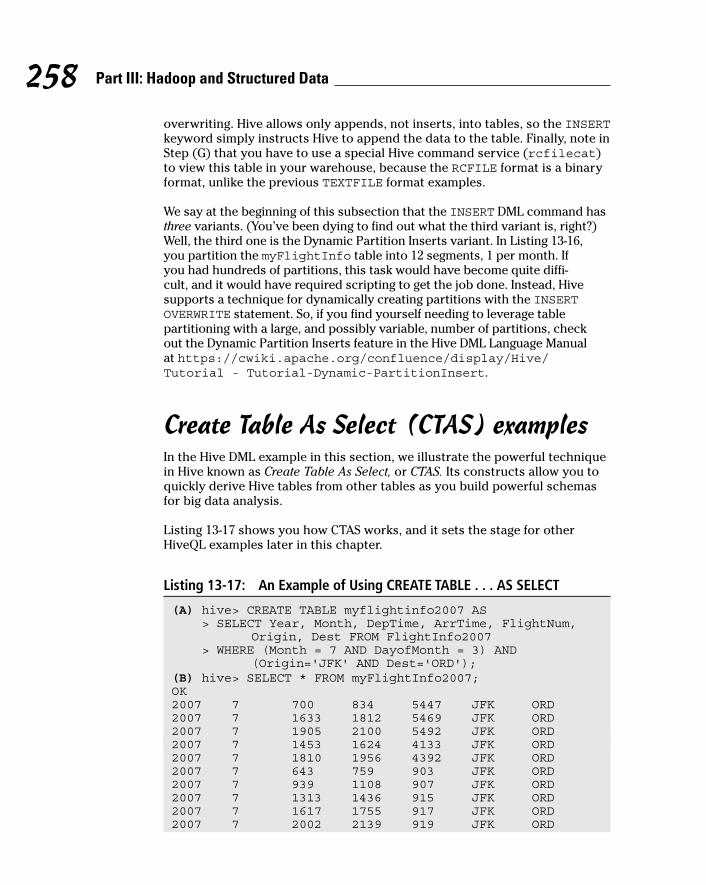
Create Table As Select (CTAS) examplesIn the Hive DML example in this section, we illustrate the powerful technique in Hive known as Create Table As Select, or CTAS. Its constructs allow you to quickly derive Hive tables from other tables as you build powerful schemas for big data analysis.
Listing 13-17 shows you how CTAS works, and it sets the stage for other HiveQL examples later in this chapter.
Listing 13-17: An Example of Using CREATE TABLE . . . AS SELECT
(A) hive> CREATE TABLE myflightinfo2007 AS > SELECT Year, Month, DepTime, ArrTime, FlightNum,
Origin, Dest FROM FlightInfo2007 > WHERE (Month = 7 AND DayofMonth = 3) AND
(Origin='JFK' AND Dest='ORD');(B) hive> SELECT * FROM myFlightInfo2007;OK2007 7 700 834 5447 JFK ORD2007 7 1633 1812 5469 JFK ORD2007 7 1905 2100 5492 JFK ORD2007 7 1453 1624 4133 JFK ORD2007 7 1810 1956 4392 JFK ORD2007 7 643 759 903 JFK ORD2007 7 939 1108 907 JFK ORD2007 7 1313 1436 915 JFK ORD2007 7 1617 1755 917 JFK ORD2007 7 2002 2139 919 JFK ORD
259 Chapter 13: Applying Structure to Hadoop Data with Hive
Time taken: 0.089 seconds, Fetched: 10 row(s)hive> CREATE TABLE myFlightInfo2008 AS > SELECT Year, Month, DepTime, ArrTime, FlightNum,
Origin, Dest FROM FlightInfo2008 > WHERE (Month = 7 AND DayofMonth = 3) AND
(Origin='JFK' AND Dest='ORD');hive> SELECT * FROM myFlightInfo2008;OK2008 7 930 1103 5199 JFK ORD2008 7 705 849 5687 JFK ORD2008 7 1645 1914 5469 JFK ORD2008 7 1345 1514 4392 JFK ORD2008 7 1718 1907 1217 JFK ORD2008 7 757 929 1323 JFK ORD2008 7 928 1057 907 JFK ORD2008 7 1358 1532 915 JFK ORD2008 7 1646 1846 917 JFK ORD2008 7 2129 2341 919 JFK ORDTime taken: 0.186 seconds, Fetched: 10 row(s)
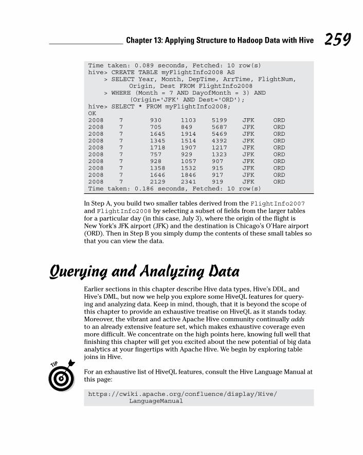
In Step A, you build two smaller tables derived from the FlightInfo2007 and FlightInfo2008 by selecting a subset of fields from the larger tables for a particular day (in this case, July 3), where the origin of the flight is New York’s JFK airport (JFK) and the destination is Chicago’s O’Hare airport (ORD). Then in Step B you simply dump the contents of these small tables so that you can view the data.
Querying and Analyzing DataEarlier sections in this chapter describe Hive data types, Hive’s DDL, and Hive’s DML, but now we help you explore some HiveQL features for query-ing and analyzing data. Keep in mind, though, that it is beyond the scope of this chapter to provide an exhaustive treatise on HiveQL as it stands today. Moreover, the vibrant and active Apache Hive community continually adds to an already extensive feature set, which makes exhaustive coverage even more difficult. We concentrate on the high points here, knowing full well that finishing this chapter will get you excited about the new potential of big data analytics at your fingertips with Apache Hive. We begin by exploring table joins in Hive.
For an exhaustive list of HiveQL features, consult the Hive Language Manual at this page:
https://cwiki.apache.org/confluence/display/Hive/LanguageManual
260 Part III: Hadoop and Structured Data
Joining tables with HiveYou probably know already that experts in relational database modeling and design typically spend a lot of their time designing normalized databases, or schemas. Database normalization is a technique that guards against data loss, redundancy, and other anomalies as data is updated and retrieved. The experts follow a number of rules to arrive at a normalized database, but Rule 1 is that you must end up with a group of tables. (One large table storing all your data is not normal — pun intended.) There are exceptions, depending on the use case, but the law of many tables is generally followed closely, especially for databases that support transactions or analytic processing (business intelligence, for example). When you begin to query and analyze your data, tables are joined based on the defined relationships between them using SQL — which means that the disks are ultimately busy on your server when you start joining tables, and busy disks usually result in slower user response times. However, the good news is that RDBMSs and EDWs are tuned to make joins as fast as possible.
What does all this have to do with joins in Hive? Well, remember that the underlying operating system for Hive is (surprise!) Apache Hadoop: MapReduce is the engine for joining tables, and the Hadoop File System (HDFS) is the underlying storage. It’s all good news for the user who wants to create, manage, and analyze large tables with Hive. The potential to unlock information that’s hidden in massive data structures is exciting. However, joins with Hive usually don’t perform as well as they do in the RDBMS/EDW world, so first-time users are often surprised by the “pokiness” of the system response. Remember that MapReduce and HDFS are optimized for through-put with big data analytics and that, in this world, latencies — user response times, in other words — are usually high. Hive is designed for batch-style analytic processing, not for fast online transaction processing. Users who want the best possible performance with SQL on Apache Hadoop have solu-tions available, and we look at those solutions in more detail in Chapter 14. For now, keep this dynamic in mind when you start joining tables with Hive. Also note that Hive architects usually denormalize their databases to some extent, so having fewer larger tables is commonplace. That’s why complex data types such as STRUCTs and ARRAYs are provided. You can use these complex data types to pack a lot more data into a single table. Because Hive table reads and writes via HDFS usually involve very large blocks of data, the more data you can manage altogether in one table, the better the overall performance.
Disk and network access is a lot slower than memory access, so minimize HDFS reads and writes as much as possible.
With this background information in mind, you can tackle making joins with Hive. Fortunately, the Hive development community was realistic and understood that users would want and need to join tables with HiveQL.
261 Chapter 13: Applying Structure to Hadoop Data with Hive
This knowledge becomes especially important with EDW augmentation, as explained in Chapter 10. Use cases such as “queryable” archives often require joins for data analysis.
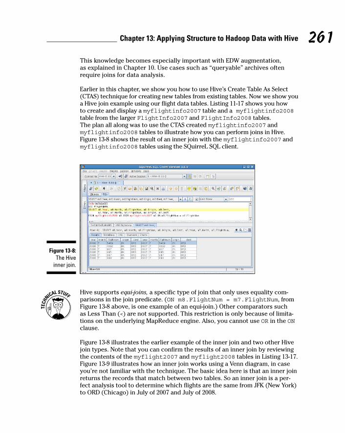
Earlier in this chapter, we show you how to use Hive’s Create Table As Select (CTAS) technique for creating new tables from existing tables. Now we show you a Hive join example using our flight data tables. Listing 11-17 shows you how to create and display a myflightinfo2007 table and a myflightinfo2008 table from the larger FlightInfo2007 and FlightInfo2008 tables. The plan all along was to use the CTAS created myflightinfo2007 and myflightinfo2008 tables to illustrate how you can perform joins in Hive. Figure 13-8 shows the result of an inner join with the myflightinfo2007 and myflightinfo2008 tables using the SQuirreL SQL client.
Figure 13-8: The Hive
inner join.
Hive supports equi-joins, a specific type of join that only uses equality com-parisons in the join predicate. (ON m8.FlightNum = m7.FlightNum, from Figure 13-8 above, is one example of an equi-join.) Other comparators such as Less Than (<) are not supported. This restriction is only because of limita-tions on the underlying MapReduce engine. Also, you cannot use OR in the ON clause.
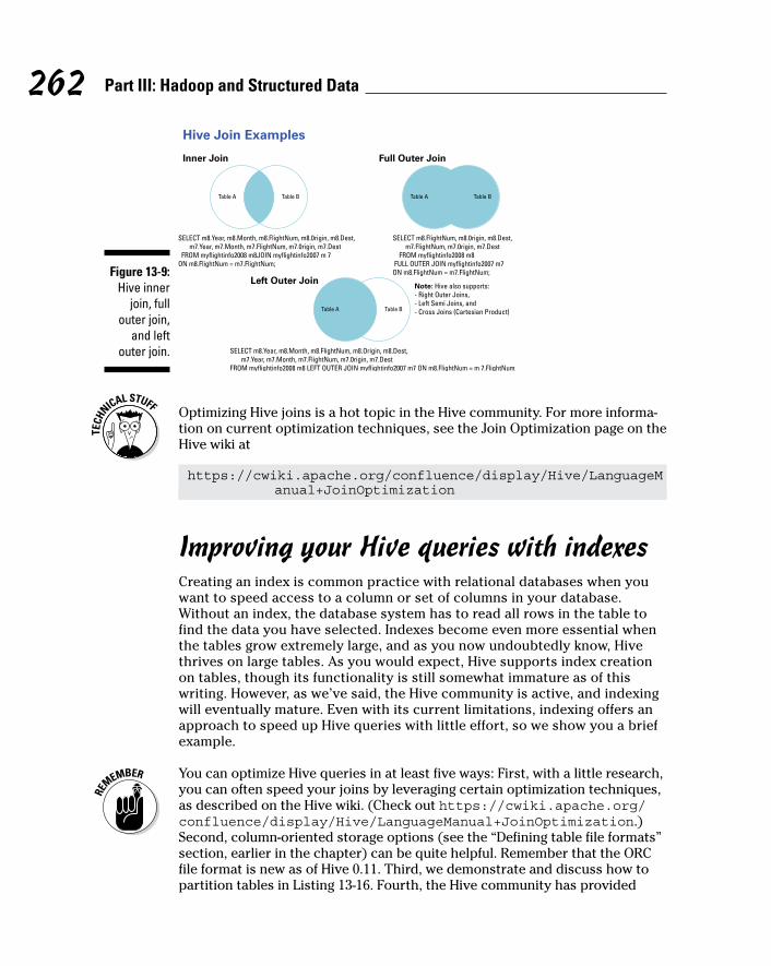
Figure 13-8 illustrates the earlier example of the inner join and two other Hive join types. Note that you can confirm the results of an inner join by reviewing the contents of the myflight2007 and myflight2008 tables in Listing 13-17. Figure 13-9 illustrates how an inner join works using a Venn diagram, in case you’re not familiar with the technique. The basic idea here is that an inner join returns the records that match between two tables. So an inner join is a per-fect analysis tool to determine which flights are the same from JFK (New York) to ORD (Chicago) in July of 2007 and July of 2008.
262 Part III: Hadoop and Structured Data
Figure 13-9: Hive inner
join, full outer join,
and left outer join.
Optimizing Hive joins is a hot topic in the Hive community. For more informa-tion on current optimization techniques, see the Join Optimization page on the Hive wiki at
https://cwiki.apache.org/confluence/display/Hive/LanguageManual+JoinOptimization
Improving your Hive queries with indexesCreating an index is common practice with relational databases when you want to speed access to a column or set of columns in your database. Without an index, the database system has to read all rows in the table to find the data you have selected. Indexes become even more essential when the tables grow extremely large, and as you now undoubtedly know, Hive thrives on large tables. As you would expect, Hive supports index creation on tables, though its functionality is still somewhat immature as of this writing. However, as we’ve said, the Hive community is active, and indexing will eventually mature. Even with its current limitations, indexing offers an approach to speed up Hive queries with little effort, so we show you a brief example.
You can optimize Hive queries in at least five ways: First, with a little research, you can often speed your joins by leveraging certain optimization techniques, as described on the Hive wiki. (Check out https://cwiki.apache.org/confluence/display/Hive/LanguageManual+JoinOptimization.) Second, column-oriented storage options (see the “Defining table file formats” section, earlier in the chapter) can be quite helpful. Remember that the ORC file format is new as of Hive 0.11. Third, we demonstrate and discuss how to partition tables in Listing 13-16. Fourth, the Hive community has provided
263 Chapter 13: Applying Structure to Hadoop Data with Hive
indexing, as illustrated in Listing 13-18. Finally, don’t forget the hive.exec.mode.local.auto configuration variable we mention earlier, in the section “Seeing How the Hive Data Manipulation Language Works.”
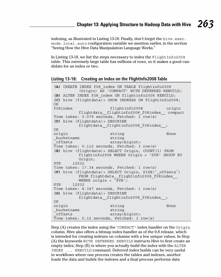
In Listing 13-18, we list the steps necessary to index the FlightInfo2008 table. This extremely large table has millions of rows, so it makes a good can-didate for an index or two.
Listing 13-18: Creating an Index on the FlightInfo2008 Table
(A) CREATE INDEX f08_index ON TABLE flightinfo2008 (Origin) AS 'COMPACT' WITH DEFERRED REBUILD;
(B) ALTER INDEX f08_index ON flightinfo2008 REBUILD;(C) hive (flightdata)> SHOW INDEXES ON FlightInfo2008;OKf08index flightinfo2008 origin
flightdata__flightinfo2008_f08index__ compactTime taken: 0.079 seconds, Fetched: 1 row(s)(D) hive (flightdata)> DESCRIBE
flightdata__flightinfo2008_f08index__;OKorigin string None_bucketname string_offsets array<bigint>Time taken: 0.112 seconds, Fetched: 3 row(s)(E) hive (flightdata)> SELECT Origin, COUNT(1) FROM
flightinfo2008 WHERE Origin = 'SYR' GROUP BY Origin;
SYR 12032Time taken: 17.34 seconds, Fetched: 1 row(s)(F) hive (flightdata)> SELECT Origin, SIZE(`_offsets`)
FROM flightdata__flightinfo2008_f08index__ WHERE origin = 'SYR';
SYR 12032Time taken: 8.347 seconds, Fetched: 1 row(s)(G) hive (flightdata)> DESCRIBE
flightdata__flightinfo2008_f08index__;OKorigin string None_bucketname string_offsets array<bigint>Time taken: 0.12 seconds, Fetched: 3 row(s)
Step (A) creates the index using the ‘COMPACT' index handler on the Origin column. Hive also offers a bitmap index handler as of the 0.8 release, which is intended for creating indexes on columns with a few unique values. In Step (A) the keywords WITH DEFERRED REBUILD instructs Hive to first create an empty index; Step (B) is where you actually build the index with the ALTER INDEX ... REBUILD command. Deferred index builds can be very useful in workflows where one process creates the tables and indexes, another loads the data and builds the indexes and a final process performs data
264 Part III: Hadoop and Structured Data
analysis. (For more on workflows — more specifically, Oozie workflows — check out Chapter 9. As of this writing, Hive doesn’t provide automatic index maintenance, so you need to rebuild the index if you overwrite or append data to the table. Also, Hive indexes support table partitions, so a rebuild can be limited to a partition. (Refer to Listing 13-16 for more information on partitions.) Step (C) illustrates how you can list or show the indexes created against a particular table. Step (D) illustrates an important point regarding Hive indexes: Hive indexes are implemented as tables. This is why you need to first create the index table and then build it to populate the table. Therefore, you can use indexes in at least two ways:
✓ Count on the system to automatically use indexes that you create.
✓ Rewrite some queries to leverage the new index table (as we demon-strate in Listing 13-18).
The automatic use of indexes is progressing, but this aspect is a work in prog-ress. Focusing on the second option, in Step (E) you write a query that seeks to determine how many flights left the Syracuse airport during 2008. To get this information, you leverage the COUNT aggregate function. You can see that Hive took 17.32 seconds on our virtual machine to report that 12,032 flights originated from Syracuse, New York. In Step (F), you leverage the new index table and use the SIZE function instead. Step (F) makes more sense after you study Step (D): Step (D) shows you what an index table looks like, where records each hold the column _bucketname, which is the location of the data in the Hive warehouse (/home/biadmin/Hive/warehouse, in this case), and an _offsets array, which is the index into the table (FlightInfo2008) in this case. So now the query in Step (F) makes sense. All Hive has to do is find the SYR origin (for Syracuse) in the flightdata__flightinfo2008_f08index__ table and then count the rows in the _offsets’ array to get the number of flights — a simple yet elegant way to double the performance (8.347 secs in Step (F) versus 17.34 in Step (E)) of the original query.
Windowing in HiveQLThe concept of windowing, introduced in the SQL:2003 standard, allows the SQL programmer to create a frame from the data against which aggregate and other window functions can operate. HiveQL now supports windowing per the SQL standard. Examples are quite helpful when explaining windowing and aggregate functions, so we start with an introductory example.
In our experience (and as other frequent flyers can attest), departure delays come with the territory when flying is your chosen mode of travel. It comes as no surprise, then, that the RITA-compiled flight data includes this information. One question we had when we first discovered this data set was, “What exactly is the average flight delay per day?” So we created a query in Listing 13-19 that produces the average departure delay per day in 2008.
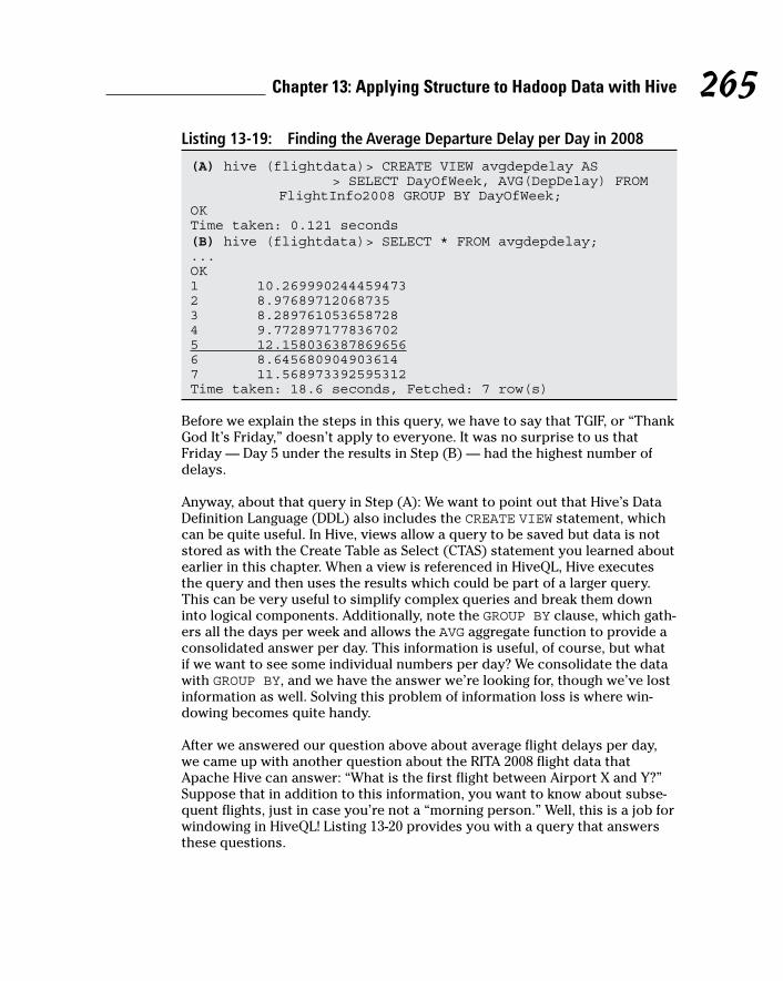
265 Chapter 13: Applying Structure to Hadoop Data with Hive
Listing 13-19: Finding the Average Departure Delay per Day in 2008
(A) hive (flightdata)> CREATE VIEW avgdepdelay AS > SELECT DayOfWeek, AVG(DepDelay) FROM
FlightInfo2008 GROUP BY DayOfWeek;OKTime taken: 0.121 seconds(B) hive (flightdata)> SELECT * FROM avgdepdelay;...OK1 10.2699902444594732 8.976897120687353 8.2897610536587284 9.7728971778367025 12.1580363878696566 8.6456809049036147 11.568973392595312Time taken: 18.6 seconds, Fetched: 7 row(s)
Before we explain the steps in this query, we have to say that TGIF, or “Thank God It’s Friday,” doesn’t apply to everyone. It was no surprise to us that Friday — Day 5 under the results in Step (B) — had the highest number of delays.
Anyway, about that query in Step (A): We want to point out that Hive’s Data Definition Language (DDL) also includes the CREATE VIEW statement, which can be quite useful. In Hive, views allow a query to be saved but data is not stored as with the Create Table as Select (CTAS) statement you learned about earlier in this chapter. When a view is referenced in HiveQL, Hive executes the query and then uses the results which could be part of a larger query. This can be very useful to simplify complex queries and break them down into logical components. Additionally, note the GROUP BY clause, which gath-ers all the days per week and allows the AVG aggregate function to provide a consolidated answer per day. This information is useful, of course, but what if we want to see some individual numbers per day? We consolidate the data with GROUP BY, and we have the answer we’re looking for, though we’ve lost information as well. Solving this problem of information loss is where win-dowing becomes quite handy.
After we answered our question above about average flight delays per day, we came up with another question about the RITA 2008 flight data that Apache Hive can answer: “What is the first flight between Airport X and Y?” Suppose that in addition to this information, you want to know about subse-quent flights, just in case you’re not a “morning person.” Well, this is a job for windowing in HiveQL! Listing 13-20 provides you with a query that answers these questions.
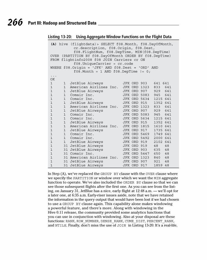
266 Part III: Hadoop and Structured Data
Listing 13-20: Using Aggregate Window Functions on the Flight Data
(A) hive (flightdata)> SELECT f08.Month, f08.DayOfMonth, cr.description, f08.Origin, f08.Dest, f08.FlightNum, f08.DepTime, MIN(f08.DepTime)
OVER (PARTITION BY f08.DayOfMonth ORDER BY f08.DepTime)FROM flightinfo2008 f08 JOIN Carriers cr ON
f08.UniqueCarrier = cr.codeWHERE f08.Origin = 'JFK' AND f08.Dest = 'ORD' AND
f08.Month = 1 AND f08.DepTime != 0;...OK1 1 JetBlue Airways JFK ORD 903 641 6411 1 American Airlines Inc. JFK ORD 1323 833 6411 1 JetBlue Airways JFK ORD 907 929 6411 1 Comair Inc. JFK ORD 5083 945 6411 1 Comair Inc. JFK ORD 5634 1215 6411 1 JetBlue Airways JFK ORD 915 1352 6411 1 American Airlines Inc. JFK ORD 1323 833 6411 1 JetBlue Airways JFK ORD 907 929 6411 1 Comair Inc. JFK ORD 5083 945 6411 1 Comair Inc. JFK ORD 5634 1215 6411 1 JetBlue Airways JFK ORD 915 1352 6411 1 American Airlines Inc. JFK ORD 1815 1610 6411 1 JetBlue Airways JFK ORD 917 1735 6411 1 Comair Inc. JFK ORD 5469 1749 6411 1 Comair Inc. JFK ORD 5492 2000 6411 1 JetBlue Airways JFK ORD 919 2102 6411 31 JetBlue Airways JFK ORD 919 48 481 31 JetBlue Airways JFK ORD 903 635 481 31 Comair Inc. JFK ORD 5447 650 481 31 American Airlines Inc. JFK ORD 1323 840 481 31 JetBlue Airways JFK ORD 907 921 481 31 JetBlue Airways JFK ORD 917 1859 48
In Step (A), we’ve replaced the GROUP BY clause with the OVER clause where we specify the PARTITION or window over which we want the MIN aggregate function to operate. We’ve also included the ORDER BY clause so that we can see those subsequent flights after the first one. As you can see from the list-ing, on January 31, JetBlue has a nice, early flight at 12:48 a.m. — we’ll opt for a later one, at 6:35 a.m. Early-riser issues aside, note that we have retained the information in the query output that would have been lost if we had chosen to use a GROUP BY clause again. This capability alone makes windowing a powerful feature, and there’s more. Along with windowing in the Hive 0.11 release, the community provided some analytics functions that you can use in conjunction with windowing. Also at your disposal are these functions: RANK, ROW_NUMBER, DENSE_RANK, CUME_DIST, PERCENT_RANK, and NTILE. Finally, don’t miss the use of JOIN in Listing 13-20: It’s a real-life,
267 Chapter 13: Applying Structure to Hadoop Data with Hive
practical example of an inner join in which we join the FlightInfo2008 table with the Carriers table to get the airline name — rather than the cryptic code found in the FlightInfo2008 table.
At the beginning of this chapter, we make the point that Hive is a key com-ponent of EDW augmentation. By importing, transforming, and analyzing the RITA flight data, we demonstrate how an EDW augmentation workflow might take shape. If data in your RDBMS or EDW can be enhanced by this flight data, Hive is the enabling technology to augment your existing IT system. Similarly, data from your RDBMS or EDW could have been exported to Apache Hive (perhaps using Apache Sqoop, as discussed in Chapter 13) and joined with this new flight data.
Other key HiveQL featuresIf this chapter is to be complete, we cannot leave a few other HiveQL features unmentioned. The following list summarizes them for you:
✓ Security: Apache Hive provides a security subsystem that can be quite helpful in preventing accidental data corruption or compromise among trusted members of workgroups. However, as of this writing, the Hive Language Manual clearly states that the Hive Security subsystem isn’t designed to prevent nefarious users from compromising a Hive system. Hive security can be established for individual users, groups, and admin-istrative roles. Hive provides privileges that can be granted or revoked to users, groups, or administrative roles. The Hive 0.10 release improved security in multi-user environments by providing authorization to the metastore, and future Hive releases will provide increasing integration with the Hadoop security framework. Kerberos is emerging as the tech-nology of choice for securing Apache Hadoop.
✓ Multi-User Locking: Hive supports multi-user warehouse access when configured with Apache Zookeeper. Without this support, one user may read a table at the same time another user is deleting that table — which is, obviously, unacceptable. (For more information on Apache Zookeeper, see Chapter 12.) Multi-user access is enabled via configura-tion variables in the hive-site.xml file. Once configured, Hive implicitly acquires locks through Zookeeper for certain table operations. Users can also explicitly manage locks in the Hive CLI. Locks and associated configuration properties/variables are described in the Hive Language Manual.
✓ Compression: Data compression can not only save space on the HDFS but also improve performance by reducing the overall size of input/output operations. Additionally, compression between the Hadoop
268 Part III: Hadoop and Structured Data
mappers and reducers can improve performance, because less data is passed between nodes in the cluster. Hive supports intermediate com-pression between the mappers and reducers as well as table output compression. Hive also understands how to ingest compressed data into the warehouse. Files compressed with Gzip or Bzip2 can be read by Hive’s LOAD DATA command.
✓ Functions: HiveQL provides a rich set of built-in operators, built-in func-tions, built-in aggregate functions, and built-in table-generating func-tions. Several examples in this chapter use built-in operators as well as built-in aggregate functions ( AVG, MIN, and COUNT, for example). To list all built-in functions for any particular Hive release, use the SHOW FUNCTIONS HiveQL command. You can also retrieve information about a built-in function by using the HiveQL commands DESCRIBE FUNCTION function_name and DESCRIBE FUNCTION EXTENDED function_name. Using the EXTENDED keyword sometimes returns usage examples for the specified built-in function. Additionally, Hive allows users to create their own functions, called user-defined functions, or UDFs. Using Hive’s Java-based UDF framework, you can create additional functions, including aggregates and table-generating functions. This feature is one of the reasons that Hive can function as an ETL tool.