Unit 3 Computer Applications - Mrs. Klein€¦ · Unit 3 Computer Applications Spreadsheet Projects Database Projects Presentation Projects ... Wizard • Add chart and axis titles

Unit 3Computer Applications

Spreadsheet ProjectsDatabase ProjectsPresentation ProjectsWeb Projects

227

Spreadsheet Projects

Project 1 Working with Budgets (240 minutes) . . . . . . . . . . . . . . . . . . . . . . . . . . . . . 229

Project 2 Calculating Loans, Payments, and Interest (320 minutes) . . . . . . . . . . . . . . 239

Project 3 Creating School-Related Spreadsheets (330 minutes) . . . . . . . . . . . . . . . . . 253

Project 4 Managing the Application Process (255 minutes) . . . . . . . . . . . . . . . . . . . . 265

Project 5 Managing Stocks and Investments (315 minutes) . . . . . . . . . . . . . . . . . . . . 279

Project 6 Using Advanced Applications (240 minutes) . . . . . . . . . . . . . . . . . . . . . . . . 291

228

O B J E C T I V E S

• Create a personal budget spreadsheet• Enter labels, values, formulas, and functions• Sort data• Format cells• Save a spreadsheet• Enter a comment• Prepare a custom footer• Preview and print a spreadsheet• Prepare and format column charts using the Chart

Wizard• Add chart and axis titles

Project 1 � Working with Budgets

Data Files: None

In this project, you will complete a variety of activities that require you todevelop and use a number of spreadsheets related to budgets. In the variousactivities, you will build spreadsheets for budgeting, enter budget data, pre-pare charts, link worksheets, and perform what-if analyses.

Activity 1 � Build the Personal Budget Worksheet

Objectives

• Create a personal budget spreadsheet• Enter labels, values, formulas, and functions• Sort data• Format cells• Save a spreadsheet• Enter a comment

Completion Time: 45 minutes

Directions

1. Open your spreadsheet program and begin a new spreadsheet.2. Enter the headings (i.e., Week 1, etc.) and labels for expenses (i.e.,

Allowance, etc.) as shown in Figure 1-1 on the following page.

Unit 3 � Spreadsheet Projects � Project 1 229

• Add and name worksheets• Enter data into a new worksheet• Copy and paste an entire spreadsheet• Add a custom footer• Enter labels, functions, and formulas• Link data• Use AutoFormat• Change the result of a formula or function to a value• Perform what-if analyses• Use the Goal Seek function

Vocabulary

BudgetFunds availableExpensesBalance forwardMonthly summaryBalance

Tip

You can quickly copy datainto adjacent cells by clickingand dragging on the fill han-dle of a cell.

230 Unit 3 � Spreadsheet Projects � Project 1

Copyright 2006 Thomson Learning/South-Western

3. Format the cells as Number cells with two decimal places. Insert a sin-gle underline under the last item to be summed in each section.

4. Enter the SUM function for the Total Funds Available and Total Expensesrows, as well as the Monthly Summary column. (Note: When calculatingthe Monthly Summary for Total Funds Available, you will need to modifythe formula to subtract the amount brought forward each month.That extraamount is not additional income; it represents funds not spent and carried for-ward from the previous month.)

5. Key the following comment in the cell for the Monthly Summary: Youmust subtract the balance brought forward from the previousmonth when calculating the Total Funds Available, since theseare not additional funds.

6. Enter a formula to calculate the Balance by subtracting Total Expensesfrom Total Funds Available.

7. Enter a formula to calculate the Percent of Budget Used. You will need todivide the Total Expenses by the Total Funds Available. (Note: An errormessage, such as #DIV/0!, will be displayed in cells with this formula unlessyou include an IF function that keeps the cell blank under specified conditions(i.e., =IF(B14>0,B31/B14,"")) ).

8. If the expense types (i.e.,Allowance, etc.) are not already in alphabeticalorder, sort them by letter.

9. Using the Tools drop-down menu, check all spelling in the spread-sheet.

10. Save the spreadsheet as ssp1a1xx (ss = spreadsheets, p1 = project 1,a1 = activity 1, xx = your initials).

Figure 1-1 Budget Spreadsheet

Help Index

Enter keywords:

Merge and split cellsEnter functionsEnter formulasSave a fileFormat cell(s)

Activity 2 � Enter Data into Personal Budget Spreadsheet

Objectives

• Enter data in a worksheet• Prepare a custom footer• Preview a worksheet• Print a worksheet


Directions

1. Open the spreadsheet you completed in Activity 1, ssp1a1xx.2. Enter the following data for each budget week.

Week 1 Week 2 Week 3 Week 4

Allowance 20.00 20.00 20.00 20.00Balance Forward 8.50 8.10 10.31 26.96Earnings 56.00 59.55 57.10 65.95Financial Gifts 0.00 10.00 0.00 0.00Miscellaneous 0.00 0.00 0.00 0.00

Expenses

Cell Phone 0.00 21.34 0.00 0.00Charity 0.00 0.00 3.00 0.00Clothing 11.05 0.00 15.95 0.00Entertainment 16.50 22.10 11.00 32.00Food and snacks 5.00 8.00 7.50 9.00Gas/fuel for car 10.00 12.50 13.00 18.00Gifts 0.00 0.00 0.00 12.50Gym fees 0.00 14.00 0.00 14.00Magazine Subscriptions 0.00 0.00 0.00 23.95Miscellaneous 2.00 3.50 0.00 0.00Music, CDs 21.85 0.00 0.00 0.00Placed in savings 5.00 5.00 5.00 5.00Video/DVD rentals 3.00 0.00 3.00 0.00

3. If your spreadsheet is accurate, your Total Funds Available for the monthshould total 338.60 and the Monthly Summary Balance should be 4.86. Ifyou did not get these results, check your entries for accuracy, as well asall formulas and functions.

4. Add a custom footer with your name left-aligned, Project 1 centered,and Activity 2 right-aligned as shown below.

Your Name Project 1 Activity 2



Vocabulary

Page SetupPrint PreviewFooter

Tips

You can access the Header/Footer toolbar from the Viewmenu. Select the Switch be-tween header/footer but-ton to add a header or footer.

You can access the PageSetup dialog box from theFile menu.



5. Using the Print Preview function, preview your spreadsheet to verifycorrect placement of your footer.

6. Print a copy of your worksheet.7. Save your spreadsheet as ssp1a2xx.

Activity 3 � Prepare Charts

Objectives

• Prepare column charts using the Chart Wizard• Add chart and axis titles• Format charts• Name worksheets


Directions

1. Open the spreadsheet you completed in Activity 2, ssp1a2xx.2. Using the guidelines below and the Chart Wizard, prepare two charts.

One chart will show funds available for the month and one will displayexpenses for the month, based on the totals for each category.a. Use a Column chart type.b. Use the data from the Monthly Summary column in ssp1a2xx.c. Add chart titles and X and Y axis titles, as shown in Figures 1-2 and

1-3 on the following page.d. Use different colors for the Funds and Expenses columns.e. Place each chart on a separate worksheet. Name the worksheets

January Funds and January Expenses.f. Save your workbook as ssp1a3xx.

Help Index

Enter keywords:

Printing

Vocabulary

Column chartWorkbookWorksheet (spreadsheet)

Tip

Right-click anywhere on achart to display the pop-upmenu.

You can access the ChartWizard by clicking the Chart Wizard button on the Formatting toolbar or fromthe Insert menu.

Help Index

Enter keywords:

Creating charts



Figure 1-2 January Funds Available

Figure 1-3 January Expenses



Activity 4 � Enter Data into a New Worksheet

Objectives

• Add a worksheet• Enter data into a new worksheet• Copy and paste an entire spreadsheet• Add a custom footer• Preview and print a spreadsheet


Directions

1. Open the workbook you saved in Activity 3, ssp1a3xx.2. Add a new worksheet and name it February.3. Copy the entire January worksheet and paste it onto the new February

worksheet.4. Delete all numeric values and enter the February data shown in Figure

1-4.

Vocabulary

Worksheet tab

Tip

Use the Select All button lo-cated to the left of column Aand above row 1 to select anentire spreadsheet.

Select All button

Figure 1-4 February Values



Help Index

Enter keywords:

Add or remove sheetRename a sheet

Vocabulary

LinkingAutoFormat

5. If your spreadsheet is accurate, your Total Funds Available for the monthshould be 341.70 and the Monthly Summary Balance should be 0.79. Ifyou did not get these results, check your entries for accuracy, as well asall formulas and functions.

6. Add a footer like the one you used in Activity 3, but specify Activity 4.7. Preview your worksheet to ensure that the footer displays correctly.8. Print a copy of your worksheet.9. Save your spreadsheet as ssp1a4xx.

Activity 5 � Link Worksheets

Objectives

• Add worksheets• Enter labels, functions, and formulas• Link data• Use AutoFormat


In Activity 5, you will link and summarize the budget funds and expendi-tures for January and February.

Directions

1. Open the spreadsheet you completed in Activity 4, ssp1a4xx.2. Add a new worksheet and name it January-February Summary.3. Enter the labels as shown in Figure 1-5, on the following page.4. Enter the appropriate formulas to link the Monthly Summary

amounts for January and February to each source of funds or expenses.Asample formula for linking is as follows:

=SUM(January!F8)+(February!F8)5. Enter the appropriate formulas to calculate the totals, balances, and

percentages. Balances brought forward are not included in total fundsavailable.

6. Use AutoFormat to format your spreadsheet like the oneshown in Figure 1-5.

7. Save your spreadsheet as ssp1a5xx.

Tips

When linking data in cells,you can quickly point to andclick a cell or range of cellsto select a reference, ratherthan manually keying cell references.

You can save time by copyingand pasting labels used onother worksheets.

Help Index

Enter keywords:

Creating links



Figure 1-5 January-February Summary



Activity 6 � Use Goal Seek

Objectives

• Change the result of a formula or function to a value• Perform what-if analyses• Use the Goal Seek function


The funds and expenditures in your budget don’t allow for any additionalexpenses or increases in savings, since you are spending nearly all of youravailable funds. In this activity, you will use Goal Seek to automaticallymodify your budget to limit the percent of funds used to 90 percent.

Directions

1. Open your Activity 5 worksheet, ssp1a5xx.2. Add two new worksheets and name them Goal Seek 1 and Goal

Seek 2.3. Copy the Activity 5 worksheet onto these two new sheets.4. Save your workbook as ssp1a6xx.5. Go to the Goal Seek 1 worksheet. Using the Paste Special function,

change the necessary numeric cell contents to values. (Note: The cell inwhich you are setting a value must contain a formula; the cell you are changing toachieve the desired value must contain a value.) The Paste Special dialogbox is shown in Figure 1-6.

Vocabulary

What-if analysisGoal SeekValue

Figure 1-6 Paste Special Dialog Box

Tip

To change the result of a for-mula in a cell to a value, usethe Paste Special option.

Help Index

Enter keywords:

Performing what-if analysis ona worksheet



6. Use Goal Seek to determine the total funds you would have needed inyour January and February budgets to keep the percent of the budgetspent at 90 percent. (See Figure 1-7.)

Figure 1-7 Goal Seek

7. Once you achieve the desired results, save your worksheet again.8. Go to the Goal Seek 2 worksheet. Using the Paste Special function,

change the necessary numeric cell contents to values. Use Goal Seek todetermine how much you would have to reduce total expenses to keepthe percent of the budget spent to 90 percent.

9. Once you achieve the desired results, save your worksheet again.

O B J E C T I V E S

• Format and add patterns to cells• Use the PMT (Payment) function• Enter formulas• Lock cells and protect worksheets• Add comments• Make loan decisions and complete loan

calculations• Integrate spreadsheets and word processing• Determine the monthly payment for a mortgage• Use Page Setup to change the page orientation of

a spreadsheet• Add worksheets• Print and save a worksheet

Project 2 � Calculating Loans, Payments, and Interest

Data Files: None

In this project, you will build worksheets that will enable you to determinemonthly payments for various types of loans.You will identify the cost ofvarious loan options and select the best option for financing based on vari-ous scenarios.

Activity 1 � Build the Loan Worksheet

Objectives

• Format cells• Add patterns to cells• Use the PMT (Payment) function• Enter formulas• Lock cells and protect worksheets• Add comments



• Link data from another worksheet• Determine amount of principal and interest included

in a payment• Determine the total interest paid on a mortgage• Determine the interest paid for a specific period of

the loan• Calculate the percentage of principal paid each year• Calculate the payoff amount for a mortgage• Combine functions and formulas• Use the Freeze Pane function• Determine equity in an investment• Look up specific months

Vocabulary

Interest ratePaymentAbsolute valueRelative value



Directions

1. Open a new worksheet.2. Enter the labels and format cells for color or patterns as shown in

Figure 2-1.

Tip

To convert a negative value toa positive value, use the ABSfunction. This function returnsthe absolute value of a num-ber, without a positive or negative sign.

Help Index

Enter keywords:

ABS

3. Format the Loan Amount cell as currency, with no dollar sign and twodecimals.

4. Format the Annual Interest Rate cell as a percentage with two decimals.5. Format the Loan Period in Years cell as a number with no decimal places.6. Enter the Payment (PMT) function into the Monthly Payment cell.The

PMT function requires that you make three entries, as shown in Figure2-2 on the following page:• Rate (annual interest rate): Since you are determining monthly pay-

ment, you will need to use a formula to divide the rate by 12, asshown in Figure 2-3.

• Nper (total number of payments): Since the loan is expressed inyears, you will need to use a formula to multiply the number of yearsin the loan period by 12, as shown in Figure 2-3 on the followingpage.

• Pv: Present value of the loan (loan amount).A sample PMT function is =PMT(D5/D12,D6*12,D4).

7. Format the cell for Number of Payments as a number with no decimalplaces. Enter a formula to calculate the total number of payments.

8. Format the cell for Total Cost of the Loan as currency, with a dollar signand two decimal places. Enter the appropriate formula to calculate thetotal cost of the loan, including interest, as shown in Figure 2-4 on page242. (Note: You will need to add the ABS (absolute function) to generate apositive number since the monthly payment is enclosed in parentheses and inter-preted as a negative number.A sample formula would be =ABS(D8*D9).)

9. Format the cell for Total Interest Paid as currency, with a dollar sign andtwo decimal places. Enter the appropriate formula to calculate the totalinterest.

Figure 2-1 Activity 1



10. Enter the comments shown in Figures 2-3 to 2-5 (on this page and thefollowing page) for the cell labels Monthly Payment and Total Cost of theLoan, as well as the cell containing the Monthly Payment amount.

11. Lock the cells containing formulas and functions and protect the work-sheet for locked and unlocked cells without a password.

12. Save the worksheet as ssp2a1xx (ss = spreadsheets, p2 = project 2, a1 =activity 1, xx = your initials).

Figure 2-2 PMT Dialog Box

Figure 2-3 Monthly Payment Cell Comment



Figure 2-4 Total Cost of the Loan Comment

Figure 2-5 Monthly Payment Comment

Activity 2 � Analyze the Expense of Borrowing MoneyThis is an integrated activity and requires students to participate in activedecision making.

Objectives

• Complete loan calculations• Make loan decisions• Integrate spreadsheets and word processing


Directions

Open the Cost of Loan spreadsheet you prepared in Activity 1, ssp2a1xx,and use that worksheet to determine the total cost of a loan for purchasinga car at the cost of $23,850, given the following three scenarios:

Scenario 1:1. Loan amount: $23,8502. Annual interest rate: 4.5%3. Loan period in years: 64. Save your completed worksheet as ssp2a2axx.

Scenario 2:1. Loan amount: $23,8502. Annual interest rate: 4.2%3. Loan period in years: 54. Save your completed worksheet as ssp2a2bxx.

Scenario 3:1. Loan amount: $23,8502. Annual interest rate: 3.5%3. Loan period in years: 44. Save your completed worksheet as ssp2a2cxx.

Decision-Making ActivityAssume that you have just been given your first job and that your annualincome is $33,500.You do not have an automobile, but you have a goodjob and a good credit rating.You need to purchase an automobile and areapproved for the loans identified in Scenarios 1–3 above. Prepare a work-sheet for each scenario to determine the total cost of each of the loan op-tions. Select one of the options and prepare a one-page report (using yourword processing program) explaining why you selected that option. Paste acopy of the worksheet representing the scenario you selected as a pictureinto your report. Save your report as ssp2a2dxx.



Vocabulary

Total cost of loanTotal interest

Tip

Select the Paste Specialfunction to access a varietyof formats for pasting copiedmaterial.

Help Index

Enter keywords:

CopyPastePaste special



Activity 3 � Analyze the Cost of a Mortgage

Objectives

• Determine the monthly payment for a mortgage• Determine the interest paid for a specific loan payment• Change the page orientation of your spreadsheet• Print and save a worksheet


A mortgage is a lien against property in which the borrower is givenmoney and the property is used as collateral for the loan. (A loan usuallyrequires the payment of interest in exchange for use of the money.)Mortgages generally span a longer period of time than other types of loans,often 10 to 30 years or more.The interest paid for most mortgages is tax-deductible.

In this activity, you will build a spreadsheet that calculates the interestcosts for a mortgage over various periods of time.

Directions

1. Open a new spreadsheet.2. Open your spreadsheet from Activity 1, ssp2a1xx, and unprotect the

worksheet.3. Copy the appropriate range of cells as shown in Figure 2-6, and paste

the range into cell A1 of the new spreadsheet.

Vocabulary

MortgageLienLoanCollateralPresent valueTax-deductibleOrientationIPMT function

Tip

Use the fill handle to quicklycopy data to a range of cells.

Help Index

Enter keywords:

IPMTAbsolute referenceRelative referenceOrientation

Figure 2-6 Range to Copy

4. Enter the following values into their respective cells:• Loan amount: $100,000• Annual interest rate: 9.5%• Loan period in years: 20

5. Change the title from Determining the Cost of a Loan to Cost ofMortgage.Add the labels shown in row 8.Your worksheet should looksimilar to Figure 2-7 on the following page.

6. The mortgage in this example spans 20 years, or 240 monthly pay-ments. It is important to be able to calculate the interest paid for a spe-cific period of time, such as the first or second year, so that you canidentify the amount of interest that can be used for a tax deduction.Perform this calculation by using the IPMT function.

7. Use the fill handle to enter the month numbers into the appropriatecolumns, as shown below.

B D F H J L1 – 40 41 – 80 81 – 120 121 – 160 161 – 200 201 – 240

8. Enter the IPMT function in the cell to the right of Month 1.TheIPMT function requires the following four entries, as shown in the dia-log box displayed in Figure 2-8. (Note: It is important to use absolute andrelative cell references so you can copy this function to other cells.)• Rate: should reference the cell with the interest rate• Per: should reference the cell indicating the month• Nper: should reference the cell with the number of payments• Pv: should reference the cell with the amount mortgaged



Figure 2-7 Cost of Mortgage Worksheet

Figure 2-8 PMT Dialog Box

9. The amount of interest paid in Month 1 of the mortgage should be$791.67. If you got this result, copy the IPMT formula into the cells formonths 2 to 240. If you did not get the correct result, check your for-mula. (A partial worksheet is shown in Figure 2-9 on the followingpage.)



Figure 2-9 Partial Solution

10. Lock any cells containing formulas or functions and protect the work-sheet. Name the worksheet Activity 3.

11. Print a copy of the worksheet, changing the orientation to Landscapeand modifying it to fit on a single page.

12. Save your worksheet as ssp2a3xx.

Activity 4 � Calculate the Cost of a Mortgage

Objectives

• Add a worksheet• Link data from another worksheet• Determine amount of principal included in a payment• Determine amount of interest included in a payment• Determine total interest paid on a mortgage• Determine interest paid for a specific period of the loan


Directions

1. Open the spreadsheet from Activity 3, ssp2a3xx.2. Add a new worksheet and name it Yearly Interest.3. Copy the range of cells A1:A7 from the Activity 3 worksheet to the

Yearly Interest worksheet, leaving row 8 blank as shown in Figure 2-10on the following page.

4. In row A9, enter the label Total Interest.5. In the range A10:A29, enter the labels Year 1, Year 2, Year 3, etc.,

ending with Year 20.6. In the range B10:B29, enter the total interest paid for each year by

linking to that information in the Activity 3 worksheet.7. In the range C10:C29, enter the absolute values of the numbers in the

range B10:B29.8. Center the headings in rows 1 and 9 to span columns A, B, and C.

Vocabulary

PrincipalInterestTax deduction

Help Index

Enter keywords:

ABS

Tip

Hold down Ctrl when select-ing ranges in differentcolumns.

9. Fill row 8, columns A–C with a color.10. In cell A31, enter the label Total Interest. In cell B31, enter the appro-

priate SUM formula to calculate the total interest. In C31, enter theappropriate SUM function to calculate the absolute value of the totalinterest.

11. In cell A32, enter the label Total Payments. In cell B32, enter a for-mula to calculate the sum of the total payments. In cell C32, enter theabsolute value of cell B32.

12. In cell A33, enter the label Interest Percentage of Total Paid.13. In cell C33, enter a formula to calculate the interest percentage of the

total amount paid for the mortgage.14. Format cell C33 as a percentage with two decimal places. Format all

other cells in the range B10:B32 and C10:C32 as currency, with twodecimals and a dollar sign.

15. If your spreadsheet is accurate, the total interest paid for the mortgageshould be $123,711.49. If you did not get this amount, check yourspreadsheet for errors.




Figure 2-10 Cost of Mortgage



Activity 5 � Pay Off a Mortgage

Objectives

• Calculate principal and interest of each payment• Calculate payoff amount for a mortgage• Combine functions and formulas• Use the Freeze Pane function• Use Page Setup


Directions

1. Open your spreadsheet from Activity 4, ssp2a4xx.2. Add a new worksheet and name it Payoff Amount.3. Insert two new columns as needed to display the principal and balance

of the loan after each payment, similar to that shown in Figure 2-11 onthe following page.

4. Enter a formula in the appropriate cells (in the Principal column) to cal-culate the amount of each payment that represents the amount of prin-cipal paid.This amount is equal to the monthly payment less theamount of interest paid that month. (Note: An efficient way to do thiswould be to insert a formula within the ABS function and to use absolute refer-ences where necessary.After entering the first formula, you can use the Copy andPaste functions or the fill handle to quickly fill in the rest of the cells.)

5. Enter a formula in the appropriate cells (in the Balance column) to cal-culate the balance of the loan after each monthly payment is made.Youwill need to subtract the amount of the payment that represents princi-pal paid from the amount of the loan remaining at the beginning of themonth. (Note: After entering the first formula, you can use the Copy andPaste functions or the fill handle to quickly fill in the rest of the cells.)

6. If your spreadsheet is accurate, the balance after payment 12 should be$98,239.06.The balance after the final payment (240) should be $0.00.If you did not get these results, check the formulas in your spreadsheet.

7. Freeze the panes after the column showing the months and below theInterest, Principal, and Balance column headings. Scroll down to ensurethat the column headers still appear.

8. Use Page Setup to change the page orientation to Landscape and fit thespreadsheet to a single page.

9. Preview the spreadsheet and then print a copy of it.10. Save the spreadsheet as ssp2a5xx.

Vocabulary

PrincipalPayoff amount

Tip

When you use a functionsuch as the ABS function, adialog box prompts you toenter required data (argu-ments). In addition to enteringdata, you can also use formu-las as arguments.

Help Index

Enter keywords:

ABSFunctionsFormulasFreeze panePage setup



Fig

ure

2-1

1P

ayo

ff A

mo

un

t S

pre

adsh

eet

(par

tial

sh

eet)



Activity 6 � Analyze the Mortgage Process

Objectives

• Calculate the percentage of principal paid each year• Calculate the payoff amount for a mortgage at the end of a specified year• Determine interest paid on a mortgage for a specified year• Determine equity in an investment• Look up specific months


Directions

1. Open the spreadsheet from Activity 5, ssp2a5xx.2. Beginning at row 50, add a new section with the labels and format

shown in Figure 2-12 on the following page. Use wordwrap as neces-sary so that all text displays.

3. In cells C52:C56, enter formulas to determine the percentage of prin-cipal that will be paid off at the end of each year specified. If your formula is accurate, the amount of principal paid off at the end of Year 1 should be 1.76%.

4. In cells C58:C60, enter formulas to determine the payoff amount at theend of each year specified. If your formula is accurate, the amount ofthe payoff at the end of Year 3 should be $94,175.53.

5. In cells C62:C65, enter formulas to calculate the amount of interestpaid during each specified period of time. If your formula is accurate,the amount of interest paid during Year 1 should be $9,424.64.

6. In cells C67:C69, enter formulas to determine the equity acquired foreach specified year. If your formula is accurate, the amount of equityacquired at the end of Year 5 should be $30,734.61.

7. Save your spreadsheet as ssp2a6axx.8. Print only the new section of your worksheet.9. Add a new worksheet and name it Look Up Data. Copy your

ssp2a6axx worksheet onto the new worksheet.10. In the Look Up Data worksheet, delete the data you added for

Activity 6. Cut and paste the repeating columns for Month, Interest,Principal, and Balance so they appear in columns B, C, D, and E, asshown in Figure 2-13 on page 252.

11. Enter the label shown in E3, using wordwrap to display all text in thecell.

12. Cell F3 should be left blank, allowing you to enter the number of themonth you want to look up.

13. In cell G3, enter a formula with the VLOOKUP function to calculatethe balance of the loan based on the month entered in F3.

Vocabulary

AppreciateEquityWordwrapVLOOKUP

Tip

Use parentheses to encloseoperations to be completedprior to other calculations in a formula.

Help Index

Enter keywords:

OperatorsFormat cellsAlignmentPrintVLOOKUP

14. Enter various months in cell F3 to be sure the VLOOKUP function isworking properly. (You can check it against the figures shown in theBalance column.)

15. Save your spreadsheet as ssp2a6bxx.



Figure 2-12 Analyses Questions



Figure 2-13 VLOOKUP Function

O B J E C T I V E S

• Write formulas with nested functions• Lock cells• Protect a worksheet• Print a selection of a worksheet• Save a spreadsheet as a template• Enter data into a template• Print a selected area of a worksheet• Work with cell borders and patterns• Use the Page Setup function• Split cells• Combine functions

Project 3 � Creating School-Related Spreadsheets

Data Files: None

In this project, you will build various school-related worksheets, which willperform such functions as estimating and tracking grades, attendance, andvarious class-related activities.

Activity 1 � Prepare a Grade Tracking Spreadsheet

Objectives

• Write formulas with nested functions• Lock cells• Protect a worksheet• Print a selection of a worksheet• Save a spreadsheet as a template


Directions

1. Open a new spreadsheet.2. As shown in Figure 3-1 on the following page, enter the labels in the

upper and lower sections of the spreadsheet. Be sure to format thenumbers as shown.

3. Format the cells in the Credit Hours column as numbers with one deci-mal place. Enter the SUM function in the appropriate cell (C18) to cal-culate the total credit hours taken.


• Apply advanced formatting• Enter data into an Attendance Records spreadsheet• Fit records to a single page• Change the page orientation of spreadsheets• Use functions (including HLOOKUP) and formulas• Use drawing tools• Enter student records• Find and filter records• Save a spreadsheet• Print a spreadsheet

Vocabulary

GPATemplateNested functions

Tip

When entering required argu-ments in a function such asthe IF function, entering “” forthe THEN portion of the for-mula will leave the cell blankif that argument is true.



Tip

You can combine the IF func-tion with the AVG function to keep a cell blank for a specific argument.

Help Index

Enter keywords:

IF functionVLOOKUP functionTemplatesCreating formulas

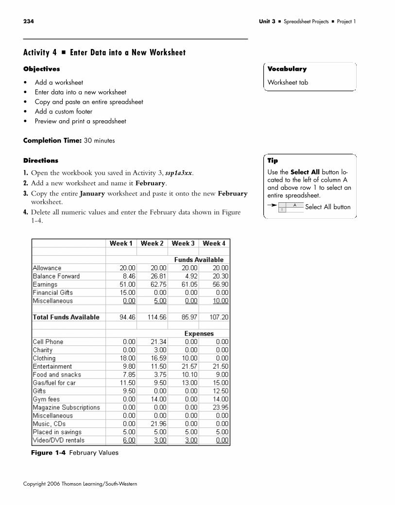
4. Format the cells in the Current Percent column as percentages withoutdecimal places. Enter the AVG function in the appropriate cell (D18) toaverage the percentages for all classes.

5. Format the cells in the GPA column as numbers with one decimalplace. Enter the VLOOKUP function in the appropriate cells (E7:E16)to look up the GPAs based on the percentage scale from the appropri-ate table in the lower section of the worksheet. Enter the AVG functionin the appropriate cell (E18) to average the GPA. Format this cell as apercentage with no decimal place.

6. In the Grade column, enter the VLOOKUP function in the appropriatecells (F7:F16, F18) to look up the grades based on the percentage scalefrom the appropriate table in the lower section of the worksheet. For-mat the column to center the grades.

7. In the Comments column, enter the VLOOKUP function in the appro-priate cells (G7:G16, G18) to look up the comment based on the Cur-rent Percent.

8. For all VLOOKUP functions, add an IF statement to ensure that thecells remain blank if no percentage is entered.

9. Format the spreadsheet so values can be entered for the Student Name,up to ten Classes, the GPA for each class, and the Current Percentagefor each class. Lock all other cells and protect the worksheet.

Figure 3-1 Tracking Grades Worksheet

10. Save the worksheet as ssp3a1xx, as a template with an .xlt extension (ss = spreadsheets, p3 = project 3, a1 = activity 1, xx = your initials).

11. Print the entire spreadsheet, then print only the top section of thespreadsheet.

Activity 2 � Enter Data for Tracking Grades

Objectives

• Enter data into a template• Save a spreadsheet• Print a spreadsheet• Print a selected area of a worksheet


Directions

1. Open the spreadsheet template (ssp3a1xx) you completed in Activity 1.2. In the top portion of the spreadsheet, enter the information from the

first grade-tracking worksheet shown below and on the following page.Save the spreadsheet as ssp3a2axx.

3. Fill out the spreadsheet with the information from the second and thirdgrade-tracking worksheets, saving each separately as ssp3a2bxx andssp3a2cxx.

4. Print a copy of the top section of each grade-tracking sheet.

Name: Antoinette Dorazio

Class Credit Hours Current Percent

English Composition I 1 72

American Literature 1 79

Algebra I 1 69

American History 1 87

Music .5 92

Art .5 97

Spanish I 1 77



Vocabulary

Template

Tip

To print a specific area of aspreadsheet, select the range,and then select File, Print,and click Selection in thePrint Dialog box.

Help Index

Enter keywords:

Print options



Name: Randy Hutchinson



Biology 1 70

Algebra I 1 83

Business Technology 1 92

Recreational Sports .5 75

Marching Band .5 95

Economics 1 62

World Literature 1 56

Name: Tomeka Brown



American Literature 1 63

Algebra I 1 58

American History 1 72

Music .5 90

Art .5 98

Spanish I 1 52

Biology 1 71

Activity 3 � Create Attendance Records

Objectives

• Work with cell borders• Work with patterns• Use the Page Setup function• Split cells• Combine functions• Apply advanced formatting


Directions

1. Open a new worksheet.2. Enter the labels and patterns as shown in the worksheet in Figure 3-2,

on the following page.3. In the Attendance Record section of this worksheet, use the COUNT

function to calculate the number of times a student was present, tardy,had an excused absence, or had an unexcused absence.

4. In the Totals row, use the SUM function to total the number of times astudent was present, tardy, excused, or unexcused.

5. Lock all cells that have labels, patterns, and formulas and protect theworksheet.

6. Change the page orientation to Landscape.7. Save your spreadsheet as ssp3a3xx.



Vocabulary

Cell patternsSplitting cellsMerging cellsFill cellsLandscape orientation

Tip

You can remove the linesused to identify rows andcolumns by changing the fillcolor of a cell or cells towhite.

You can add a border aroundmultiple cells by selecting arange of cells and adding aborder. If you didn’t changethe fill color to white, you willneed to merge the cells first.

Help Index

Enter keywords:

COUNT functionMerge or split cellsFormat cells



Fig

ure

3-2

Stu

den

t A

tten

dan

ce R

eco

rd

Activity 4 � Enter Attendance Records

Objectives

• Enter data into an Attendance Records spreadsheet• Fit records to a single page• Change the page orientation of spreadsheets• Print records


Directions

1. Open the ssp3a3xx spreadsheet that you created in Activity 3.2. Enter the records for the individual shown in Figure 3-3. Save your

spreadsheet as ssp3a4axx.



Tip

Before printing, you canchange the page orientation(and Scaling settings) by ac-cessing the Page Setup dialog box from the Filedrop-down menu.

Figure 3-3 Record 1

Help Index

Enter keywords:

Orientation

Entry Title Entry

Name Linda G. Eagley

ID 587322901

Gender F

Birth Date 6/27/89

School East High School

Grade 10

Teacher Anthony Hemandez

Room 207

Parent or Guardian Dennis P. Eagley

Relationship Father

Work Number 662-325-0938

Home Number 662-615-1919

Parent or Guardian Sandra Eagley

Relationship Mother

Work Number


Emergency Contact Mary D. Keel

Relationship Grandmother

Work Number


Dates Tardy 1/5, 1/25, 5/12, 1/7, 10/8

Dates Excused 3/7, 3/8, 3/9, 8/31, 12/15

Dates Unexcused 2/10, 11/12

3. Enter the records for each of the individuals shown in Figures 3-4 and3-5, and save these spreadsheets separately as ssp3a4bxx and ssp3a4cxx.

4. Format each worksheet to fit on a single page, then print each sheetwith a Landscape orientation.



Figure 3-4 Record 2 Figure 3-5 Record 3

Entry Title Entry

Name Heishum Lawrence

ID 482-39-2979

Gender M

Birth Date 10/12/90


Grade 10

Teacher Wylma Dickerson

Room 111

Parent or Guardian Benjamin P. Lawrence

Relationship Father



Parent or Guardian Mary Lawrence

Relationship Mother



Emergency Contact Shawn Brown

Relationship Uncle



Dates Tardy 4/14

Dates Excused 2/14, 6/1, 12/1

Dates Unexcused

Entry Title Entry

Name Josh Abrams

ID 5002-45-1991

Gender M

Birth Date 2/22/89


Grade 10

Teacher Elisabeth Burns

Room 119

Parent or Guardian Marian Collins

Relationship Grandmother



Parent or Guardian

Relationship

Work Number

Home Number

Emergency Contact Albert Abrams

Relationship Brother



Dates Tardy

Dates Excused

Dates Unexcused

Activity 5 � Create an Electronic Grade Book

Objectives

• Apply advanced formatting• Use the HLOOKUP function• Use functions and formulas• Use drawing tools• Save a spreadsheet as a template


Directions

1. Open a new spreadsheet and format cells A1:S55 as shown in Figure 3-6 on the following page.As needed, you will be required to mergeand split cells, change patterns and borders of cells, adjust cell width,and change font size.

2. Use the Arrow drawing tool to draw an arrow between lines 17 and 18as shown. Change the arrow type and line style as needed.

3. Enter the appropriate formula and functions in cell D17 to count thenumber of assignments entered. Ensure that the cell remains blank if noassignments are entered.

4. Enter the appropriate formula and functions in cell D18 to sum thetotal points for each assignment entered. Ensure that the cell remainsblank if no points are entered.

5. Enter the appropriate formula and functions in cells C24:C46 to deter-mine the total points earned for each student. Ensure that the cells re-main blank if no points were earned.

6. Enter the appropriate formula and functions in cells D24:D46 to deter-mine the percentage for each student. Ensure that the cells remainblank if no points were earned.

7. Enter the appropriate formula and functions in cells E24:E46 to lookup the GPA for each student. Ensure that the cells remain blank if nopoints were earned.

8. Enter the appropriate formulas and functions in cells F24:F46 to lookup the grade for each student. Ensure that the cells remain blank if nopoints were earned.

9. Enter some sample data to ensure that all formulas and functions areworking properly.

10. If desired, lock any cells that have fixed data or formulas and protect theworksheet.

11. Save the file as a template, ssp3a5xx.



Vocabulary

HLOOKUP functionBorderMergeSplitFunction

Tip

To remove cell borders, fill thecell with the color white.

To place a border around arange of cells with no bor-ders, select the range and se-lect Format, Cells, Border,Outline.

Help Index

Enter keywords:

Merge cellSplit cellFormat cellIF functionCOUNTHLOOKUP



Fig

ure

3-6

Gra

de

Bo

ok



Vocabulary

Ascending orderFilter

Activity 6 � Enter Grades in the Electronic Grade Book

Objectives

• Enter student records• Find records• Filter records


Directions

1. Open the spreadsheet template you created in Activity 5, ssp3a5xx.2. Enter the records as shown in Figure 3-7 on the following page.

(Note: The Total Points, Percent, GPA, and Grade columns will be calculatedautomatically.)

3. Sort the student records in ascending order by last name.4. Save the spreadsheet as ssp3a6xx.5. Delete the row separating the column headings from the student records.6. Filter the records of students who receive an A or A- and print those

records.7. Filter the records of students who have a GPA lower than 2.0 and print

those records.8. Find the records for Daniel Stumpf and Cynthia Hammer. Print only

those two records.

Tip

Be sure to select completerecords when you sort or filtera list; otherwise, the fields inthe records will be separated.

Help Index

Enter keywords:

FilterSort



Fig

ure

3-7

Stu

den

t R

eco

rds

O B J E C T I V E S

• Prepare a resume• Build a Tracking Applications spreadsheet• Insert clip art• Insert a hyperlink• Change page orientation• Fit a spreadsheet to a page• Add and name a new worksheet• Prepare a letter• Enter and update records• Use the Copy and Paste functions

Project 4 � Managing the Application Process

Data Files: High School Job Application Resume

In this project you will work with documents related to applying for a job.You will complete activities such as preparing a resume and buildingspreadsheets to compare the benefits of specific job options and to track applications you have submitted.

Activity 1 � Prepare a Resume andTracking Applications Spreadsheet

Objectives

• Prepare a resume• Build a Tracking Applications spreadsheet• Insert clip art• Insert a hyperlink• Change page orientation• Fit spreadsheet to a page

Completion time: 45 minutes

Directions

1. Open your word processing application and open the data file HighSchool Job Application Resume.doc, as shown in Figure 4-1 on the following page.


• Build a Position Comparison worksheet• Use wordwrap• Merge and split cells• Enter formulas and functions• Enter and analyze data• Add new rows• Create and format charts• Add axis and chart titles• Insert WordArt

Vocabulary

HyperlinkClip art

Tip

To replace placeholder data,highlight all the data to be replaced and begin keyingthe new data.



2. Replace the placeholder information with the following informationfor a student who will soon be graduating from high school and is beginning the application process.

Melissa Jones211 Crossgate StreetStarkville, MS 39759

662-215-0908

Professional GoalTechnical Staff Assistant while attending local college part time in theevenings.

Qualifications

Business Technology Skills

• Expert Level, Microsoft Office• Good knowledge of Windows operating system• Desktop publishing training• Keyboarding skill of 65 wpm

Communication Skills

• Member of yearbook staff• Member of debate team• Publication of three articles in the school newspaper• Senior class president speaking responsibilities

Figure 4-1 High School Job Resume

Organizational Skills

• Editor of school newspaper• Prepared various brochures and advertisements for the school’s

Future Business Leaders Association

Education

Graduation date or expected graduation date and school

• June 11, 20xx• Starkville Academy, Starkville, MS 39762

Grade Point Average and Curriculum

• GPA – 3.7• College Preparation Curriculum

Related course work

• Visual Basic• Advanced Microsoft Office Applications• Technical Writing• Business Communications• Desktop Publishing

Awards and Honors

• Senior class president• National Honor Society• State high school debate champion

Memberships and Extracurricular Activities

• National Honor Society• Debating team• Yearbook staff• Editor of school newspaper• Member FBLA

3. Save your document as ssp4a1axx (ss = spreadsheet, p4 = Project 4,a1 = Activity 1, xx = your initials).

4. Open a new spreadsheet.5. Insert clip art similar to that shown in Figure 4-2. Make the clip art

into a hyperlink to the resume you prepared (ssp4a1axx.doc).6. As shown in Figure 4-2 on the following page, freeze the panes below

the column headings and to the right of the Phone column. Change thewidth of columns to accommodate projected data. (You can adjustcolumns later as needed.)

7. Enter all labels, headings, and cell colors as shown in Figure 4-2.8. Name the worksheet Submissions.9. Change the page orientation to Landscape, and fit the spreadsheet to a

single page.10. Save the workbook as ssp4a1bxx.



Help Index

Enter keywords:

Freeze panesHyperlink



Fig

ure

4-2

Ap

plic

atio

ns

and

/or

Res

um

es S

ub

mit

ted

Activity 2 � Enter Records, Add a Worksheet, and Craft a Thank-You Letter

Objectives

• Enter records• Add a new worksheet• Name a worksheet• Prepare a letter


Directions

1. Open the worksheet you created in Activity 1, ssp4a1bxx. On the Sub-missions worksheet, enter the following records. Each record should beseparated by a shaded row.

Date: 5/10/xxPosition: Help Desk TechnicianCompany: Mississippi State UniversityContact Name: Helen YoungAddress: 100 IED Building, Starkville, MS 39762Phone: 662-325-1919Email: [email protected]: 662-325-5892Company Web Site: http://www.msstate.edu/dept/its_help/References Sent:YesStatus of Application:Comments:

Date: 5/12/xxPosition: Staff AssistantCompany:Women’s health CenterContact Name: Jacob HowellAddress: 3480 Bluecutt Road, Columbus, MS 39705Phone: 662-329-5001Email:Fax: 662-329-1878Company Web Site: www.womenshealth.netReferences sent:YesStatus of Application:Comments:



Vocabulary

RecordForm letter

Tip

A workbook is used to holdmultiple, related spreadsheetslike those you will build in thisactivity.

Help Index

Enter keywords:

Sheet tabs



Date: 5/18/xxPosition: Media SpecialistCompany: Golden Triangle Media GroupContact Name: Barry HowardAddress: 2002 Hwy 45 N, Columbus, MS 39701Phone: 662-243-9673Email:Fax: 662-243-7599Company Web Site: www.gtmedia.netReferences sent:YesStatus of application:Comments:

2. Save your spreadsheet as ssp4a2axx.3. Add a new worksheet to the workbook and name it Interviews.4. Format the Interviews spreadsheet similar to that shown in Figure 4-3

on the following page. (Note: Estimate the necessary width of the columns;you can adjust them later if necessary.)

5. Save your spreadsheet again using the same name.6. Open a blank word processing document and prepare the following

thank-you form letter (see Figure 4-4 on page 272) to be sent to eachpotential employer that grants you an interview. Save your letter asssp4a2bxx.



Fig

ure

4-3

Inte

rvie

w S

hee

t



Activity 3 � Update Records and Create a Hyperlink

Objectives

• Update and enter records• Insert clip art• Create a hyperlink• Use the Copy and Paste functions


Directions

1. Open the spreadsheet you created in Activity 2, ssp4a2axx.

Figure 4-4 Thank-You Letter

Vocabulary

Placeholder

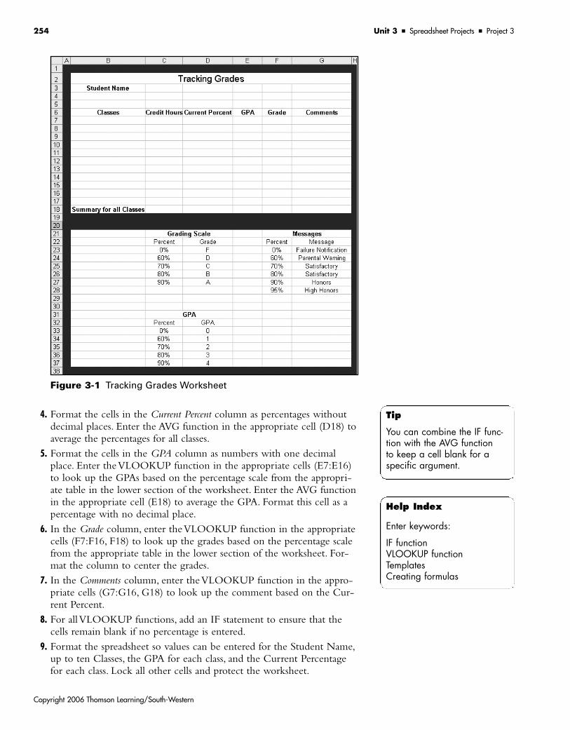
2. Add the following information to the Submission records:

Mississippi State University

Status: Called for an interview.Comments: Interview scheduled for 5/15/xx at 10:00 a.m.

Women’s Health Center

Status: Called for an interview.Comments: Interview scheduled for 5/17/xx at 9:00 a.m.

Golden Triangle Media Group

Status: Called on 5/23/xx.Comments:Application not reviewed.

Status: Received letter on 5/27/xx.Comments: Not invited for an interview.

3. Save your spreadsheet as ssp4a3axx.4. Enter the following records on the Interviews worksheet:

Date: 5/15/xxPosition: Help Desk TechnicianCompany: Mississippi State UniversityAddress: 100 IED Building, Starkville, MS 39762Interviewer: Helen YoungPhone: 662-325-1919Email: [email protected] you: SentComments:Thank you sent on 5/16/xx

Date: 5/17/xxPosition: Staff AssistantCompany:Women’s Health CenterAddress: 3480 Bluecutt Road, Columbus, MS 39705Interviewer: Jacob HowellPhone: 662-329-5001Email:Thank you: SentComments:Thank you sent on 5/18/xx

5. Save your spreadsheet again using the same name.6. Insert appropriate clip art above the Thank You heading. Format the clip

art as a hyperlink to the thank-you letter you created in Activity 2(ssp4a2bxx).

7. Save your spreadsheet again using the same name.8. Using the form letter you created in Activity 2, prepare thank-you letters

for the two interviews completed. Save the first letter as ssp4a3bxx andthe second as ssp4a3cxx.

9. Print both thank-you letters.



Tip

When entering information ina placeholder, select theplaceholder information andkey the new information.

Right-click on an email ad-dress, Web address, or hy-perlink to select the cell or towork with the data.

If you use the Copy/Pastefunctions to copy informationfrom a spreadsheet to a wordprocessing document, use theFormat Painter to change thefont when necessary.

Help Index

Enter keywords:

Format painter



Vocabulary

Position ComparisonVAR

Activity 4 � Build a Position Comparison Worksheet

Objectives

• Build a Position Comparison worksheet• Use wordwrap• Merge and split cells


Directions

1. Open a new spreadsheet.2. Enter the labels as shown in Figure 4-5 on the following page. Use

wordwrap and formatting as necessary. (Note: You will enter any necessaryformulas and functions in the next activity.)


Tip

Click the Increase Indentbutton to indent items.



Fig

ure

4-5

Po

siti

on

Co

mp

aris

on

Wo

rksh

eet

Activity 5 � Perform Statistical Analyses

Objectives

• Enter formulas and functions• Enter data• Add new rows• Analyze data


Directions

1. Open the spreadsheet you created in Activity 4, ssp4a4xx.2. Enter the appropriate formulas in cells C9:E9 to calculate the Estimated

Weekly Earnings for each position. For an employee paid hourly, youshould multiply the number of hours worked by the hourly rate. Foremployees paid a salary, you should divide the salary by 52 weeks.

3. For offer 2, the Staff Assistant position, it is estimated that you wouldwork six overtime hours per week.The overtime rate is 1.5 times thehourly rate. For salaried employees, you should divide the weekly salaryby 40 hours to get the hourly rate. Enter the appropriate formula intocell E10 to calculate the amount of overtime to be paid.

4. Enter the estimated expenses for each position, as shown in Figure 4-6.



Figure 4-6 Expenses

5. The ratings for the variables are shown in Figure 4-7. Enter these valuesinto your worksheet.

6. In the Total Points section of your worksheet, cells G41:J51, insert a newrow below the Count row to display the Variance values. Enter the ap-propriate formula to calculate the variance.

Vocabulary

MeanMedianModeCountT testVarianceMINMAX

Tip

Pay careful attention to the re-quired entries in the dialogbox displayed when you se-lect a specific function.

Help Index

Enter keywords:

VarianceTest

7. Enter all other necessary formulas to perform the functions indicated(i.e., Mean, Median, etc.) in the Total Points section.The T test functionreturns the probability that the two groups are different within a speci-fied error range.This function requires four parameters:• The range of group 1• The range of group 2• Tails (one or two distributions)• Variance (equal or unequal)

8. After making all required calculations, save your spreadsheet as ssp4a5xx.

Activity 6 � Perform Graphic Analyses

Objectives

• Create charts• Add axis and chart titles• Insert WordArt• Format charts


In this activity, you will use the total points earned for the three positionsin Activity 5 to develop a column chart similar to the one shown in Figure 4-8 on the following page.



Tip

The T test calculates the prob-ability that the two groups,such as the variables for offer1 compared to the variablesfor offer 2, are significantlydifferent within a given rangeof probability. For example,.05 would indicate there is a5 percent chance the groupsare not different, and .01would mean that there is onlya 1 percent chance thegroups aren’t different.

Figure 4-7 Job Ratings

Vocabulary

Column chartBar chartAxis

Tip

Right-click anywhere within achart to display a pop-upmenu.

Directions

1. Open the spreadsheet you created in Activity 5, ssp4a5xx.2. Add a new worksheet and name it Position Comparison. Insert the col-

umn chart and axis titles as shown in Figure 4-8.Add WordArt to thecolumns as shown.

3. Add a new worksheet and name it Income Comparison. Prepare a newbar chart based on the Estimated Weekly Earnings for each position be-fore taxes, similar to the chart shown in Figure 4-9.Add the chart andaxis title as shown.

4. Save your workbook as ssp4a6xx.



Help Index

Enter keywords:

Chart wizardWordArt

Figure 4-9 Outdoor Bar Chart

Figure 4-8 Column Chart

O B J E C T I V E S

• Build a Stock Performance spreadsheet• Enter formulas and functions• Use a variety of formatting options• Add new worksheets• Rename and arrange worksheets• Enter weekly data• Use advanced functions and formulas

Project 5 � Managing Stocks and Investments

Data Files: None

In Project 5, you will work with spreadsheets related to stock investments,performance, and analyses. Each share of stock represents a portion of theownership of a corporation.The market value of a share of stock is its cur-rent value which might be less or more than the amount paid when it waspurchased.

Activity 1 � Build a Stock Performance and Analyses Spreadsheet

Objectives

• Build a Stock Performance spreadsheet• Enter formulas and functions• Use a variety of formatting options


Directions

1. Open a new spreadsheet.2. Enter the labels and values shown in columns A:K in Figure 5-1 on the

following page.3. Format the values in the Quantity column as Numbers with no decimals.4. Format the Purchase Price, Fees Charged, Total Cost, Current Value Per Share,

Current Market Value, and Gain or Loss columns as Currency, with twodecimals and no dollar sign.

5. Format the % Gain or Loss column as a Percentage with two decimals.6. Enter an appropriate formula in column G to determine the Total Cost.


• Link data from one sheet to another• Copy and paste data• Prepare charts• Add titles and text to charts• Use logical functions• Add, delete, and sort records

Vocabulary

Stock Market value

Tip

The total cost of stock is equalto the quantity purchasedtimes the number of sharesplus any fees charged.

Help Index

Enter keywords:

Borders



Fig

ure

5-1

Sto

ck P

erfo

rman

ce A

nal

yses

7. Enter the SUM function into row 29 to total the Quantity, Fees Charged,and Total Cost columns.

8. Place a border around the cell to be used for the date entry. Format thiscell as a Date in mm/dd/yy format.

9. Save your spreadsheet as ssp5a1xx (ss = Spreadsheet, p5 = Project 5,a1 = Activity 1, xx = your initials).

Activity 2 � Create Additional Worksheets; Update and Analyze Data

Objectives

• Add new worksheets• Name worksheets• Enter weekly data


Directions

1. Open the spreadsheet you created in Activity 1, ssp5a1xx.2. Name the first worksheet Week 1.3. Add three additional worksheets to the workbook and name the sheets

Week 2, Week 3, and Week 4.4. On the Week 1 worksheet, arrange the investments alphabetically by

name.5. Copy the entire Week 1 worksheet to the Week 2,Week 3, and Week 4

sheets.6. Add a fifth worksheet as shown in Figure 5-2 on the following page.

Enter the labels and values as shown. (You can copy the investmentnames from one of the existing worksheets.) Name the worksheet StockWeekly Performance.

7. Save your workbook as ssp5a2xx.



Vocabulary

Record

Tip

Use the Select All button toselect the entire spreadsheet.

Help Index

Enter keywords:

Name sheet

Activity 3 � Analyze Investment Performance

Objectives

• Enter data• Use advanced functions and formulas• Link data from one sheet to another• Copy and paste data


Directions

1. Open the workbook you modified in Activity 2, ssp5a2xx.2. On the Week 1 worksheet, link to and/or copy and paste the market

value of the stock on 6/7/xx from the Stock Weekly Performance work-sheet to column H.

3. In column I of the Week 1 worksheet, enter an appropriate formula tocalculate the Current Market Value Per Share (Quantity � Current Market Value per share).

4. In column J, enter an appropriate formula to calculate the Gain or Loss(Current Market Value – Total Cost)

5. In column K, enter a logical function and formula to display the % Gainor Loss.

6. Enter the SUM function in the Performance Summary row to total eachcolumn. (Note: You do not need to total the Purchase Price column.)

7. Refer to Figure 5-3 on the following page to view the completed Work1 worksheet.



Figure 5-2 Stock Weekly Performance

Vocabulary

Weekly performance

Tip

You can use the ISERR func-tion to keep a cell blankunder specified conditions.

Help Index

Enter keywords:

Logical function



Fig

ure

5-3

Sto

ck P

erfo

rman

ce a

nd

An

alys

es W

eek

1

8. Repeat steps 2–8 for worksheets Week 2–4.9. Save your worksheet as ssp5a3xx.

Activity 4 � Create Charts

Objectives

• Prepare charts• Add titles to charts• Add text to charts


Directions

1. Open the spreadsheet you worked on in Activity 3, ssp5a3xx.2. Open the Chart Wizard.3. Prepare a 3-D column chart like the one shown in Figure 5-4 based on

the Week 4 worksheet. Use the Total Cost and Current Market Value cellsas the basis for the chart.

4. Add the chart and axis titles as shown in Figure 5-4.



Vocabulary

3-D column chartPie chart

Tip

To select non-adjacent rangesof cells, select the first range,hold down Ctrl, and selectthe additional ranges.

Figure 5-4 Column Chart of Growth Comparison

5. Add the abbreviated names for the stocks above the columns.6. Save the chart on a new worksheet. Name the sheet Growth

Comparison.7. If it is not still open, open the Chart Wizard.8. Prepare a pie chart like the one shown in Figure 5-5 based on the

Week 4 worksheet. Use the Current Market Value cell as the basis for thechart.

9. Add the chart title as shown in Figure 5-5.



Help Index

Enter keywords:

Chart wizardColumn chart

Figure 5-5 Distribution of Investments

10. Be sure the abbreviated stock name and the percentage of the total investment is displayed on the chart.

11. Save the chart on a new worksheet. Name the sheet Distribution ofInvestments.




Activity 5 � Perform Analyses and Logical Functions

Objectives

• Add new worksheets• Arrange worksheets• Name worksheets• Copy and paste data• Use logical functions


Directions

1. Open the spreadsheet from Activity 4, ssp5a4xx.2. Add two new worksheets and name them Week 5 and Week 6.3. Make sure the sheets in the workbook are arranged in the following

order:Week 1,Week 2,Week 3,Week 4,Week 5,Week 6, Stock WeeklyPerformance, Growth Comparison, and Distribution of Investments.

4. Add the data shown in Figure 5-6 to your Stock Weekly Performancesheet.

Vocabulary

WorkbookSheet (worksheet)Logical functions

Tip

Using “ ” in an argument in alogical function will keep thecell blank if the preceding ar-gument is not met.

Figure 5-6 Current Value Per Share

Help Index

Enter keywords:

Logical function

5. Select cell A1 in the destination worksheet. Copy and paste the entireWeek 4 worksheet onto the Week 5 and Week 6 worksheets.

6. From the Stock Weekly Performance sheet, copy the Week 5 currentstock values and paste them onto the Week 5 spreadsheet in the CurrentValue Per Share column.

7. From the Stock Weekly Performance sheet, copy the Week 6 currentstock values and paste them onto the Week 6 spreadsheet in the Cur-rent Value Per Share column.

8. As shown in Figure 5-7, add two additional columns (L and M) to yourWeek 5 and Week 6 worksheets.



Figure 5-7 Additional Columns

9. Enter an appropriate logical function in column L that will display theword Sell in red if the value in the % Gain or Loss column is less than -.15%.

10. Enter an appropriate logical function in column M that will display theword Buy in blue if the value in the % Gain or Loss column is greaterthan 15%.


Activity 6 � Add and Delete Records

Objectives

• Delete rows• Add records• Delete records• Sort records


Directions

1. Open the spreadsheet from Activity 5, ssp5a5xx.2. On the Week 6 worksheet, add a new section called Long-Term

Profit/Loss, as shown in Figure 5-8 on page 289.This section should bebelow the existing Stock Performance and Analyses section.

Vocabulary

Stock

Tip

Be sure to select completerecords when you sort them.

Help Index

Enter keywords:

Sort



3. Copy and paste the records that are to be sold as shown. Delete thoserecords from the Stock Performance and Analyses section of the work-sheet.

4. Enter the SUM function to calculate the Total Cost, Current MarketValue, and % Gain or Loss. Remove the function from the Consider Selland Consider Additional Investment columns.

5. Delete the rows where records were removed, and delete five additionalrows below the last record in the Stock Performance and Analyses section.

6. Arrange the Long-Term Profit/Loss records in alphabetical order.7. Additional shares (as shown in Figure 5-9 on the following page) were

purchased at different prices than the shares already owned.Add thesenew listings to your spreadsheet.

8. Sort the records in alphabetical order.9. Save your spreadsheet as ssp5a6xx.



Fig

ure

5-8

Lon

g-T

erm

Pro

fit/

Loss

Fig

ure

5-9

Ad

dit

ion

al S

har

es

O B J E C T I V E S

• Use the Paste Special option• Link data• Create a folder• Insert a hyperlink• Update documents with linked data• Insert clip art• Insert a text box• Group objects• Use advanced formatting• Use Page Setup

Project 6 � Using Advanced Applications

Data Files: None

As Project 6 requires integration, you must have completed Project 5 priorto beginning this project. In Project 6, you will link data and work withmacros.

Activity 1 � Link Data

Objectives

• Use the Paste Special function• Link data• Create a folder


Directions

1. Create a new folder in your file system and name it Project 6. Be sureto save all documents created in this project in the Project 6 folder.

2. Open a new workbook.3. Open the workbook from Activity 6 of Project 5, ssp5a6xx, and go to

the Week 6 worksheet.4. Copy the top section (cells A1:M24) of the first sheet and paste it onto

the first worksheet in your new workbook.5. Name the worksheet Third Quarter.


• Record, run, and assign a macro• Run a macro from a graphic• Group objects• Compose and key a letter• Process a stock liquidation• Edit and move records• Delete records• Prepare a linked letter• Prepare a letter with an embedded object

Vocabulary

Source documentDestination document

Help Index

Enter keywords:

Creating Links



Tip

Documents that are linked toother documents can be up-dated to automatically reflectchanges in the source docu-ment. You will be promptedas to whether you want thedestination document to beupdated each time it isopened. Be careful not tochange the name or locationof the source document sothat the link is not broken.

6. Close the first spreadsheet (ssp5a6xx).7. The investments in this spreadsheet have been turned over to an invest-

ment company for management.The company will send the investorquarterly statements.The value of each share of stock on September 30is shown in Figure 6-1. Update your spreadsheet to reflect these figures.

Figure 6-1 Current Investment Value Per Share

8. Save your spreadsheet as ssp6a1xx (ss = Spreadsheet, p6 = Project 6,a1 = Activity 1, xx = your initials).

9. Save a second copy of your spreadsheet as Activity 1 Solution A.Thissecond file should not be updated in the future.

10. Open a new word processing document and prepare the letter shownin Figure 6-2 on the following page.

11. Use the Paste Special function to copy your ssp6a1xx spreadsheet intothe letter as a linked worksheet object.

12. Save your letter as ssp6a1bxx.13. Save a second copy of your letter as Activity 1 Solution B.This second

file should not be updated in the future, as it will be changed to reflectthe current value of the investments.

14. Print a copy of your letter.



Figure 6-2 Letter to Investor

Activity 2 � Work with Linked Data

Objectives

• Insert a hyperlink• Update documents with linked data• Insert clip art• Insert a text box• Group objects


Directions

1. Open the spreadsheet from Activity 1, ssp6a1xx.2. Add clip art similar to that shown in Figure 6-3. Size as necessary to

place it in the upper-right corner of the spreadsheet.



Vocabulary

Text box

Figure 6-3 Clip Art

3. Add text to the clip art that says Quarter Report. Group the clip artand the text as a single object.

4. Format the clip art as a hyperlink to the letter you created in Activity 1,ssp6a1bxx.

5. Save your spreadsheet using the same name.6. The market value of the stock at the end of the fourth quarter,

December 31, is shown in Figure 6-4 on the following page. Updateyour spreadsheet with this information and save it again using the samename.

7. Save a second copy of the spreadsheet as ssp6a2axx. (Note:Yourssp6a1xx spreadsheet is linked to your word processing documents.That linkmust remain active in order for updates to be reflected in linked letters, which iswhy you must save the spreadsheet using the same name.)

8. Click your hyperlink to access your Quarter Report letter. Change thedate to December 31. (Note: The spreadsheet image that you inserted intothe document should be updated automatically to reflect the current market valueof the stock you entered into your spreadsheet.)

9. Print a copy of the letter.10. Save the letter as ssp6a2bxx.11. Save a second copy of the letter as Activity 2 Solution B, so that you

will know not to update this file.

Tip

To group objects, click thefirst object, hold down Shift,and click the second object.Next, select Group from theDrawing toolbar.

Help Index

Enter keywords:

Link data

Activity 3 � Use Advanced Formatting and Macros

Objectives

• Use advanced formatting• Use Page Setup• Record a macro• Run a macro• Group objects• Assign a macro


Directions

1. Open the spreadsheet you worked with in Activity 1, ssp6a1xx.2. Create a new worksheet in this workbook and name it Liquidation

Request. In the next few steps, you will prepare a Liquidation Requestspreadsheet similar to that shown in Figure 6-5 on the following page.

3. Add all necessary formatting, including patterns, borders, and cellmerges, as shown.

4. Format the ID cell as a Social Security Number.5. Format the Shares to Sell column as a Number with no decimal places.6. Format the Date Sold column as a Date, in the format of mm/dd/yy.7. Format the Shares Sold column as a Number with no decimal places.



Figure 6-4 Market Value of Stock

Vocabulary

Macro

Help Index

Enter keywords:

Macros



Fig

ure

6-5

Liq

uid

atio

n R

equ

est

8. Format the Purchase Price Per Share, Current Market Value Per Share, Fee atPurchase, Transaction Fee, Total Expenses, Revenue, and Profit or Losscolumns as Currency with two decimal places and no dollar sign.

9. Enter formulas in the appropriate cells (J11:J20) to calculate the Trans-action Fees.This formula should multiply the Shares Sold by .50.

10. Enter formulas in the appropriate cells (K11:K20) to calculate Total Ex-penses.This formula should calculate (Shares Sold � Purchase Price PerShare) + Fees at Purchase + Transaction Fee.

11. Enter formulas in the appropriate cells (L11:L20) to calculate Revenue.This formula should calculate Shares Sold � Current Market Value PerShare.

12. Enter formulas in the appropriate cells (M11:M20) to calculate Profitor Loss.This formula should calculate Revenue – Total Expenses.

13. Enter the SUM function in cells G22:M22 to total each column, andformat these cells as Currency with two decimal places and no dollarsign.

14. Add clip art of a printer and size to fit as shown.Add text of the wordprint on the graphic. Group the clip art and text together.

15. Record a macro that prints this Liquidation Request form.16. Use the clip art object you inserted to run the macro.17. Save the workbook as ssp6a3xx.18. Save it again as ssp6a1xx.

Activity 4 � Run a Macro; Compose and Key a Letter

Objectives

• Run a macro from a graphic• Compose and key a letter


Directions

1. Mrs. Karen Higgins (209 Crossgate Street, Starkville, MS 39759-1103)has requested a Liquidation Request form. Open the spreadsheet youcreated in Activity 3, ssp6a3xx. Go to the Liquidation Request work-sheet and click the graphic to activate your macro and print a blankform.

2. Open a blank word processing document and write a letter dated Febru-ary 19, 20xx from Janet Henderson, Investment Manager, to Mrs. Hig-gins. In the letter, you should indicate that the form is enclosed and thatshe must completed the top section, the name of the stocks, and thenumber of shares to sell. She must also sign the form.

3. Save the letter as ssp6a4xx.



Vocabulary

Liquidation

Tip

Be sure to keep all linked andreferenced documents in thesame location once they arereferenced. Otherwise, themacro or hyperlink will notwork.

Help Index

Enter keywords:

Macros



Activity 5 � Process Stock Liquidations and Run a Macro

Objectives

• Process a stock liquidation• Edit and move records• Delete records


Directions

1. Open the spreadsheet you created in Activity 3, ssp6a3xx.2. The Liquidation Request shown in Figure 6-6 on the following page

was received from Karen Higgins. Go to the Liquidation Request work-sheet and complete the document based on the information receivedfrom Mrs. Higgins and the information available on the PerformanceAnalysis worksheet located in the same workbook.The date of sale willbe 2/15/xx.The current market values of the stocks are 20.10 (StewardCommunications) and 99.8 (DACUM Telcom).

3. When you have completed the Liquidation Request, save your spread-sheet as ssp6a5xx. Save it again as ssp6a1xx.

4. Now that these stocks have been sold, you must also remove them fromthe Performance Analysis worksheet in this workbook. Leave the nameof the sold investments in the record, key the word SOLD in red in theSymbols column, and delete the remainder of the information for eachstock sold.

5. Save your spreadsheet again as ssp6a5xx and ssp6a1xx.



Fig

ure

6-6

Liq

uid

atio

n R

equ

est



Tip

When you link a document,that document is connected to the source document; any changes in the sourcedocument can be updated automatically.

When you embed a docu-ment, you can access toolsfor editing the document byclicking the object. It is notupdated automatically whenthe source document changes.

Activity 6 � Use Dynamic Data Exchange and Object Linking and Embedding

Objectives

• Prepare a linked letter• Prepare a letter with an embedded object


Directions

1. Open the spreadsheet you worked on in Activity 5, ssp6a5xx.2. Click the graphic that links to the Quarter Report letter.This will open

the letter you created in Activity 1, ssp6a1bxx.3. Prepare a letter to Mrs. Higgins with a date of February 15, 20xx.This

report is sent quarterly, as well as each time an investor sells stock.4. Save the letter as ssp6a6axx.5. Compose a second letter to Mrs. Higgins from Janet Henderson, Invest-

ment Manager, in which you explain that her liquidation request hasbeen processed. Embed a copy of the form by pasting it into the letter asa spreadsheet. Mention that a check for the revenue is also enclosed.

6. Save your letter as ssp6a6bxx.

Vocabulary

DDEOLE

Help Index

Enter keywords:

Edit linked or embedded object