UNIT 3: ANALYSIS OF AUTOMATED FLOW LINE & LINE · PDF file · 2013-03-31ANALYSIS OF AUTOMATED FLOW LINE & LINE BALANCING ... Process Technology refers to the body of knowledge about

UNIT 3:

ANALYSIS OF AUTOMATED FLOW LINE & LINE BALANCING

General Terminology & Analysis:

There are two problem areas in analysis of automated flow lines which must be addressed:

1. Process Technology 2. Systems Technology

Process Technology refers to the body of knowledge about the theory & principles of the particular manufacturing process used on the production line. E.g. in the manufacturing process, process technology includes the metallurgy & machinability of the work material, the correct applications of the cutting tools, chip control, economics of machining, machine tools alterations & a host of other problems. Many problems encountered in machining can be overcome by application of good machining principles. In each process, a technology is developed by many years of research & practice. Terminology & Analysis of transfer lines with no Internal storage:

There are a few assumptions that we will have to make about the operation of the Transfer line & rotary indexing machines:

1. The workstations perform operations such as machining & not assembly. 2. Processing times at each station are constant though they may not be equal. 3. There is synchronous transfer of parts. 4. No internal storage of buffers.

In the operation of an automated production line, parts are introduced into the first workstation & are processed and transported at regular intervals to the succeeding stations. This interval defines the ideal cycle time, Tc of the production line. Tc is the processing time for the slowest station of the line plus the transfer time; i.e. :

Tc = max (Tsi) + Tr ---------------- (1)

Tc = ideal cycle on the line (min)

Tsi = processing time at station (min)

Tr = repositioning time, called the transfer time (min)

In equation 1, we use the max (Tsi) because the longest service time establishes the pace of the production line. The remaining stations with smaller service times will have to wait for the slowest station. The other stations will be idle. In the operation of a transfer line, random breakdowns & planned stoppages cause downtime on the line. Common reasons for downtime on an Automated Production line:

1. Tool failures at workstations. 2. Tool adjustments at workstations 3. Scheduled tool charges 4. Limit switch or other electrical malfunctions.

www.bookspar.com | VTU NOTES | QUESTION PAPERS | NEWS | RESULTS | FORUMS




5. Mechanical failure of a workstation. 6. Mechanical failure of a transfer line. 7. Stock outs of starting work parts. 8. Insufficient space for completed parts. 9. Preventive maintenance on the line worker breaks.

The frequency of the breakdowns & line stoppages can be measured even though they occur randomly when the line stops, it is down for a certain average time for each downtime occurrence. These downtime occurrences cause the actual average production cycle time of the line to be longer than the ideal cycle time.

The actual average production time Tp:

Tp = Tc + FTd ------------------------ 2 F = downtime frequency, line stops / cycle Td = downtime per line stop in minutes The downtime Td includes the time for the repair crew to swing back into action, diagnose the cause of failure, fix it & restart the drive.

FTd = downtime averaged on a per cycle basis Production can be computed as a reciprocal of Tp

Rp = 1 ----------------------------- 3

Tp

Where, Rp = actual average production rate (pc / min)

Tp = the actual average production time The ideal production rate is given by

Rc = 1 ------------------------------ 4

Tc

Where Rc = ideal production rate (pc / min) Production rates must be expressed on an hourly basis on automated production lines. The machine tool builder uses the ideal production rate, Rc, in the proposal for the automated transfer line & calls it as the production rate at 100% efficiency because of downtime. The machine tool builder may ignore the effect of downtime on production rate but it should be stated that the amount of downtime experienced on the line is the responsibility of the company using the production line. Line efficiency refers to the proportion of uptime on the line & is a measure of reliability more than efficiency. Line efficiency can be calculated as follows:

E = Tc = Tc + FTd ----------------- 5

Tp Tc





Where E = the proportion of uptime on the production line. An alternative measure of the performance is the proportion of downtime on the line which is given by:

D = FTd = FTd + FTd ----------------- 6 Tp Tc Where D = proportion of downtime on the line E + D = 1.0 An important economic measure of the performance of an automated production line is the cost of the unit produced. The cost of 1 piece includes the cost of the starting blank that is to processed, the cost of time on the production line & the cost of the tool consumed. The cost per unit can be expressed as the sum of three factors: Cpc = Cm + CoTp + Ct ------------------------ 7 Where Cpc = cost per piece (Rs / pc) Cm = cost per minute to operate the time (Rs / min) Tp = average production time per piece (min / pc) Ct = cost of tooling per piece (Rs / pc) Co = the allocation of capital cost of the equipment over the service life, labour to operate the line, applicable overheads, maintenance, & other relevant costs all reduced to cost per min. Problem on Transfer line performance:

A 30 station Transfer line is being proposed to machine a certain component currently produced by conventional methods. The proposal received from the machine tool builder states that the line will operate at a production rate of 100 pc / hr at 100% efficiency. From a similar transfer line it is estimated that breakdowns of all types will occur at a frequency of F = 0.20 breakdowns per cycle & that the average downtime per line stop will be 8.0 minutes. The starting blank that is machined on the line costs Rs. 5.00 per part. The line operates at a cost for 100 parts each & the average cost per tool = Rs. 20 per cutting edge. Compute the following: 1. Production rate 2. Line efficiency 3. Cost per unit piece produced on the line Solution:

1. At 100% efficiency, the line produces 100 pc/hr. The reciprocal gives the unit time

or ideal cycle time per piece. Tc = 1 = 0.010hr / pc = 0.6 mins 100

The average production time per piece is given by:





Tp = Tc + FTd = 0.60 + 0.20 (8.0)

= 0.60 + 1.60 = 2.2 mins / piece Rp = 1 / 2.2m = 0.45 pc / min = 27 pc / hr Efficiency is the ratio of the ideal cycle time to actual production time E = 0.6 / 2.2 = 27 % Tooling cost per piece Ct = (30 tools) (Rs 20 / tool) 100 parts = Rs. 6 / piece The hourly ratio of Rs 100 / hr to operate the line is equivalent to Rs. 1.66 / min. Cpc = 5 + 1.66 (2.2) + 6 = 5 + 3.65 + 6 = Rs 14.65 / piece Upper Bound Approach:

The upper bound approach provides an upper limit on the frequency on the line stops per cycle. In this approach we assume that the part remains on the line for further processing. It is possible that there will be more than one line stop associated with a given part during its sequence of processing operations. Let Pr = probability or frequency of a failure at station i where i = 1, 2,………. η Station i where i = 1, 2, ……………. η

Since a part is not removed from the line when a station jam occurs it is possible that the part will be associated with a station breakdown at every station. The expected number of lines stops per part passing through the line is obtained by summing the frequencies Pi over the n stations. Since each of the n stations is processing a part of each cycle, then the expected frequency of line stops per cycle is equal to the expected frequency of line stops per part i.e. η F = ∑ Pi ----------------------------- 8 i = 1 where F = expected frequency of line stops per cycle Pi = frequency of station break down per cycle, causing a line stop

η = number of workstations on the line If all the Pi are assumed equal, which is unlikely but useful for computation purposes, then F = η.p where all the Pi are equal ---------------- 9 p = p = ………….. p = p 1 2 η





Lower Bound Approach:

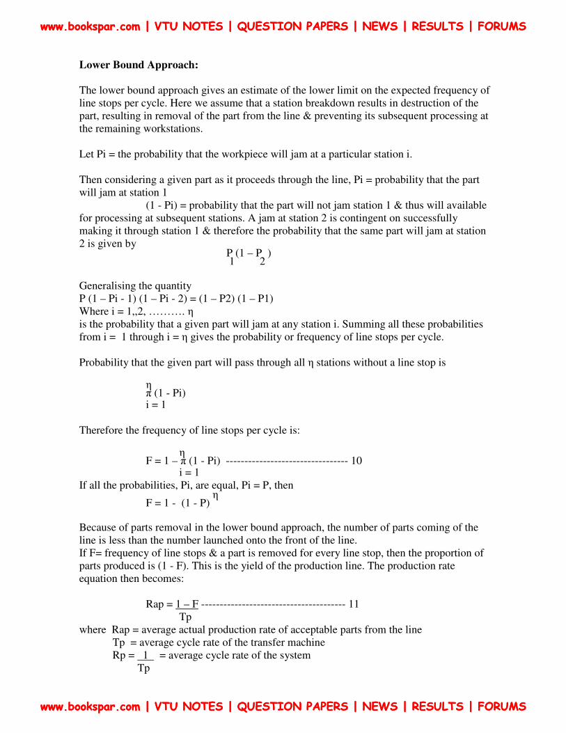
The lower bound approach gives an estimate of the lower limit on the expected frequency of line stops per cycle. Here we assume that a station breakdown results in destruction of the part, resulting in removal of the part from the line & preventing its subsequent processing at the remaining workstations. Let Pi = the probability that the workpiece will jam at a particular station i. Then considering a given part as it proceeds through the line, Pi = probability that the part will jam at station 1 (1 - Pi) = probability that the part will not jam station 1 & thus will available for processing at subsequent stations. A jam at station 2 is contingent on successfully making it through station 1 & therefore the probability that the same part will jam at station 2 is given by

P (1 – P ) 1 2

Generalising the quantity P (1 – Pi - 1) (1 – Pi - 2) = (1 – P2) (1 – P1) Where i = 1,,2, ………. η is the probability that a given part will jam at any station i. Summing all these probabilities from i = 1 through i = η gives the probability or frequency of line stops per cycle. Probability that the given part will pass through all η stations without a line stop is η π (1 - Pi) i = 1 Therefore the frequency of line stops per cycle is: η F = 1 – π (1 - Pi) --------------------------------- 10 i = 1 If all the probabilities, Pi, are equal, Pi = P, then η F = 1 - (1 - P) Because of parts removal in the lower bound approach, the number of parts coming of the line is less than the number launched onto the front of the line. If F= frequency of line stops & a part is removed for every line stop, then the proportion of parts produced is (1 - F). This is the yield of the production line. The production rate equation then becomes: Rap = 1 – F --------------------------------------- 11 Tp where Rap = average actual production rate of acceptable parts from the line Tp = average cycle rate of the transfer machine Rp = 1 = average cycle rate of the system Tp





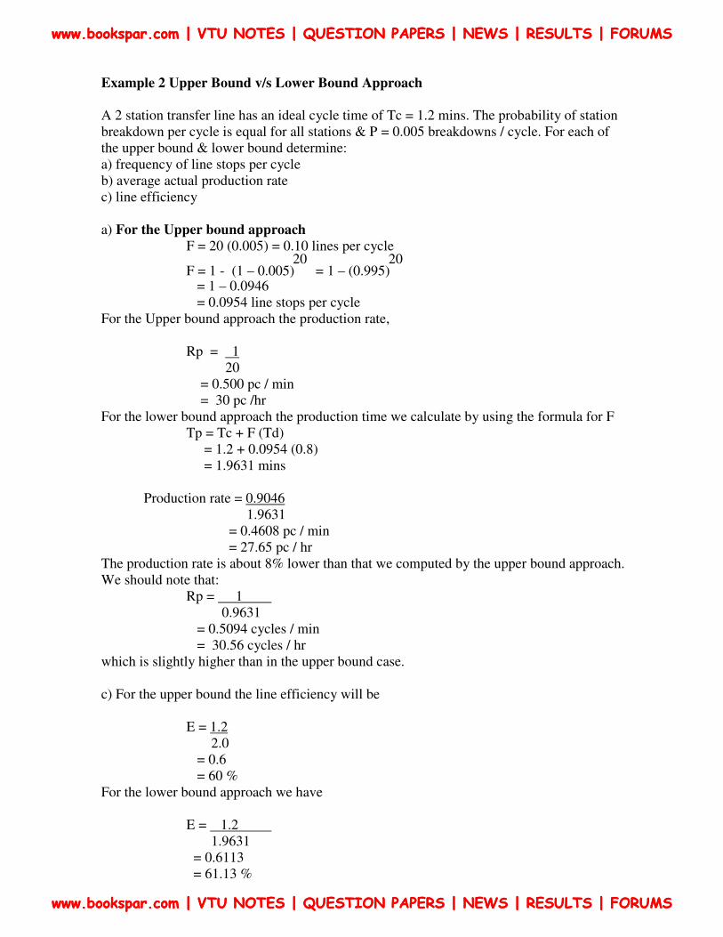
Example 2 Upper Bound v/s Lower Bound Approach

A 2 station transfer line has an ideal cycle time of Tc = 1.2 mins. The probability of station breakdown per cycle is equal for all stations & P = 0.005 breakdowns / cycle. For each of the upper bound & lower bound determine: a) frequency of line stops per cycle b) average actual production rate c) line efficiency a) For the Upper bound approach F = 20 (0.005) = 0.10 lines per cycle 20 20 F = 1 - (1 – 0.005) = 1 – (0.995) = 1 – 0.0946 = 0.0954 line stops per cycle For the Upper bound approach the production rate, Rp = 1 20 = 0.500 pc / min = 30 pc /hr For the lower bound approach the production time we calculate by using the formula for F Tp = Tc + F (Td) = 1.2 + 0.0954 (0.8) = 1.9631 mins Production rate = 0.9046 1.9631 = 0.4608 pc / min = 27.65 pc / hr The production rate is about 8% lower than that we computed by the upper bound approach. We should note that: Rp = 1 0.9631 = 0.5094 cycles / min = 30.56 cycles / hr which is slightly higher than in the upper bound case. c) For the upper bound the line efficiency will be E = 1.2 2.0 = 0.6 = 60 % For the lower bound approach we have E = 1.2 1.9631 = 0.6113 = 61.13 %





Line efficiency is greater with lower bound approach even though production rate is lower. This is because lower bound approach leaves fewer parts remaining on the line to jam. Analysis of Transfer Lines with Storage Buffers:

In an automated production line with no internal storage of parts, the workstations

are interdependent. When one station breaks down all other stations on the line are affected either immediately or by the end of a few cycles of operation. The other stations will be forced to stop for one or two reasons 1) starving of stations 2) Blocking of stations Starving on an automated production line means that a workstation is prevented from performing its cycle because it has no part to work on. When a breakdown occurs at any workstation on the line, the stations downstream from the affected station will either immediately or eventually become starved for parts.

Blocking means that a station is prevented from performing its work cycle because it cannot pass the part it just completed to the neighbouring downstream station. When a break down occurs at a station on the line, the stations upstreams from the affected station become blocked because the broken down station cannot accept the next part for processing from the neighbouring upstream station. Therefore none of the upstream stations can pass their just completed parts for work.

By Adding one or more parts storage buffers between workstations production lines can be designed to operate more efficiently. The storage buffer divides the line into stages that can operate independently for a number of cycles. The number depending on the storage capacity of the buffer

If one storage buffer is used, the line is divided into two stages. If two storage buffers are used at two different locations along the line, then a three stage line is formed. The upper limit on the number of storage buffers is to have a storage between every pair of adjacent stations. The number of stages will then be equal to the number of workstations. For an η stage line, there will be η – 1 storage buffers. This obviously will not include the raw parts inventory at the front of the line or the finished parts inventory that accumulates at the end of the line. Consider a two – stage transfer line, with a storage buffer separating the stages. If we assume that the storage buffer is half full. If the first stage breaks down, the second stage can continue to operate using parts that are in the buffer. And if the second stage breaks down, the first stage can continue to operate because it has the buffer to receive its output. The reasoning for a two stage line can be extended to production lines with more than two stages. Limit of Storage Buffer Effectiveness:

Two extreme cases of storage buffer effectiveness can be identified:

1. No buffer storage capacity at all. 2. Infinite capacity storage buffers

If we assume in our Analysis that the ideal cycle time Tc is the same for all stages considered.





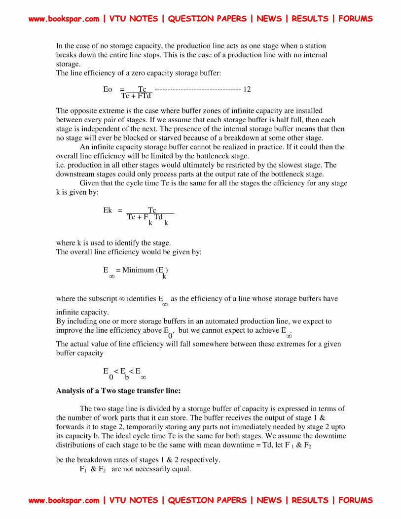
In the case of no storage capacity, the production line acts as one stage when a station breaks down the entire line stops. This is the case of a production line with no internal storage. The line efficiency of a zero capacity storage buffer: Eo = Tc --------------------------------- 12 Tc + FTd The opposite extreme is the case where buffer zones of infinite capacity are installed between every pair of stages. If we assume that each storage buffer is half full, then each stage is independent of the next. The presence of the internal storage buffer means that then no stage will ever be blocked or starved because of a breakdown at some other stage. An infinite capacity storage buffer cannot be realized in practice. If it could then the overall line efficiency will be limited by the bottleneck stage. i.e. production in all other stages would ultimately be restricted by the slowest stage. The downstream stages could only process parts at the output rate of the bottleneck stage. Given that the cycle time Tc is the same for all the stages the efficiency for any stage k is given by: Ek = Tc Tc + F Td k k

where k is used to identify the stage. The overall line efficiency would be given by: E = Minimum (E ) ∞ k where the subscript ∞ identifies E as the efficiency of a line whose storage buffers have ∞ infinite capacity. By including one or more storage buffers in an automated production line, we expect to improve the line efficiency above E , but we cannot expect to achieve E .

0 ∞ The actual value of line efficiency will fall somewhere between these extremes for a given buffer capacity E < E < E 0 b ∞ Analysis of a Two stage transfer line:

The two stage line is divided by a storage buffer of capacity is expressed in terms of the number of work parts that it can store. The buffer receives the output of stage 1 & forwards it to stage 2, temporarily storing any parts not immediately needed by stage 2 upto its capacity b. The ideal cycle time Tc is the same for both stages. We assume the downtime distributions of each stage to be the same with mean downtime = Td, let F 1 & F2 be the breakdown rates of stages 1 & 2 respectively. F1 & F2 are not necessarily equal.





Over the long run both stages must have equal efficiencies. If the efficiency of stage 1 is greater than the efficiency of stage 2 then inventory would build up on the storage buffer until its capacity is reached. Thereafter stage 1 would eventually be blocked when it outproduced stage 2. Similarly if the efficiency of stage 2 is greater than the efficiency of stage 1 the inventory would get depleted thus stage 2 would be starved. Accordingly the efficiencies would tend to equalize overtime in the two stages. The overall efficiency for the two stage line can be expressed as: 1 E = E + { D η (b) } E ------------------------- 13 b 0 1 2 where Eb = overall efficiency for a two stage line with a buffer capacity E = line efficiency for the same line with no internal storage buffer 0 1 { D η (b) } E represents the improvement in efficiency that results from having a 1 storage buffer with b > 0 when b = 0 E = Tc ----------------------------------14 0 Tc + (F + F ) Td 1 2 1 The term D can be thought of as the proportion of total time that stage 1 is down 1 1 D = F Td 1 1 ----------------------------------------- 15 Tc + (F + F ) Td 1 2

The term h (b) is the proportion of the downtime D'1 (when the stage 1 is down) that stage 2 could be up & operating within the limits of storage buffer capacity b. The equations cover several different downtime distributions based on the assumption that both stages are never down at the same time. Four of these equations are presented below: Assumptions & definitions: Assume that the two stages have equal downtime distributions (Td1 = Td2 = Td) & equal cycle times (Tc1 = Tc2 = Tc). Let F1 = downtime frequency for stage 1, & F2 = downtime frequency for stage 2. Define r to be the ration of breakdown frequencies as follows:

r = F1 ------------------- 16 F2 Equations for h(b) : With these definitions & assumptions, we can express the relationships for h(b)for two theoretical downtime distributions :





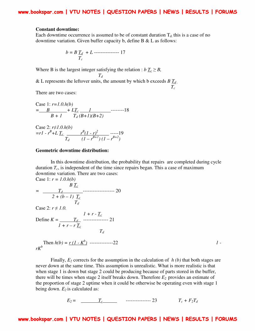
Constant downtime: Each downtime occurrence is assumed to be of constant duration Td. this is a case of no downtime variation. Given buffer capacity b, define B & L as follows: b = B Td + L --------------- 17 Tc

Where B is the largest integer satisfying the relation : b Tc ≥ B,

Td

& L represents the leftover units, the amount by which b exceeds B Td . Tc

There are two cases: Case 1: r=1.0.h(b)

= B + LTc 1 --------18

B + 1 Td (B+1)(B+2) Case 2: r≠1.0.h(b)

=r1 - rB+L Tc r

B(1 - r)

2 -----19

Td (1 – rB+1

) (1 – rB+2

)

Geometric downtime distribution:

In this downtime distribution, the probability that repairs are completed during cycle duration Tc, is independent of the time since repairs began. This a case of maximum downtime variation. There are two cases: Case 1: r = 1.0.h(b)

B Tc

= Td ------------------- 20

2 + (b – 1) Tc

Td

Case 2: r ≠ 1.0.

1 + r - Tc

Define K = Td --------------- 21

1 + r – r Tc

Td

Then h(b) = r (1 - K

b) --------------22 1 -

rKb

Finally, E2 corrects for the assumption in the calculation of h (b) that both stages are never down at the same time. This assumption is unrealistic. What is more realistic is that when stage 1 is down but stage 2 could be producing because of parts stored in the buffer, there will be times when stage 2 itself breaks down. Therefore E2 provides an estimate of the proportion of stage 2 uptime when it could be otherwise be operating even with stage 1 being down. E2 is calculated as:

E2 = Tc --------------- 23 Tc + F2Td





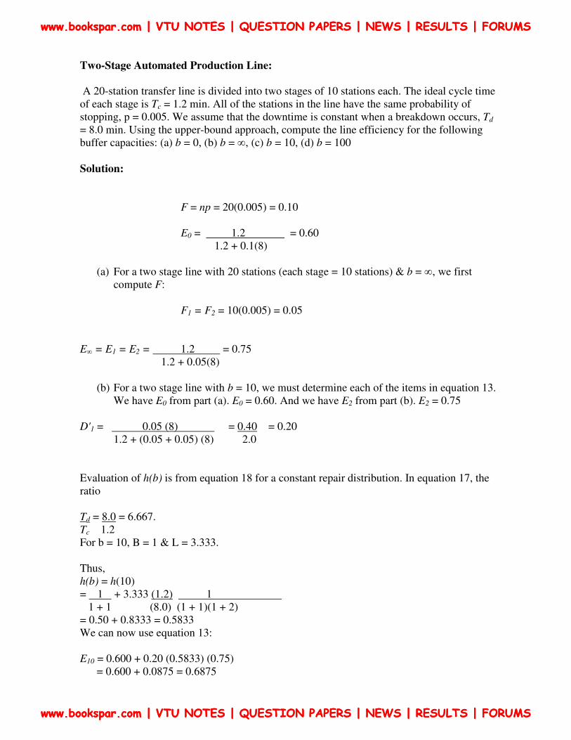
Two-Stage Automated Production Line:

A 20-station transfer line is divided into two stages of 10 stations each. The ideal cycle time of each stage is Tc = 1.2 min. All of the stations in the line have the same probability of stopping, p = 0.005. We assume that the downtime is constant when a breakdown occurs, Td = 8.0 min. Using the upper-bound approach, compute the line efficiency for the following buffer capacities: (a) b = 0, (b) b = ∞, (c) b = 10, (d) b = 100 Solution:

F = np = 20(0.005) = 0.10 E0 = 1.2 = 0.60 1.2 + 0.1(8)

(a) For a two stage line with 20 stations (each stage = 10 stations) & b = ∞, we first

compute F:

F1 = F2 = 10(0.005) = 0.05

E∞ = E1 = E2 = 1.2 = 0.75 1.2 + 0.05(8)

(b) For a two stage line with b = 10, we must determine each of the items in equation 13. We have E0 from part (a). E0 = 0.60. And we have E2 from part (b). E2 = 0.75

D'1 = 0.05 (8) = 0.40 = 0.20 1.2 + (0.05 + 0.05) (8) 2.0 Evaluation of h(b) is from equation 18 for a constant repair distribution. In equation 17, the ratio Td = 8.0 = 6.667. Tc 1.2 For b = 10, B = 1 & L = 3.333. Thus, h(b) = h(10) = 1 + 3.333 (1.2) 1 1 + 1 (8.0) (1 + 1)(1 + 2) = 0.50 + 0.8333 = 0.5833 We can now use equation 13: E10 = 0.600 + 0.20 (0.5833) (0.75) = 0.600 + 0.0875 = 0.6875





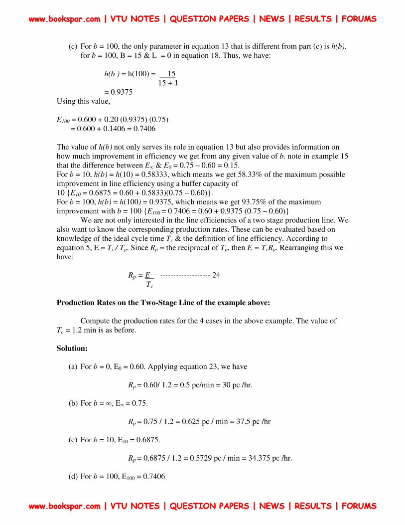
(c) For b = 100, the only parameter in equation 13 that is different from part (c) is h(b). for b = 100, B = 15 & L = 0 in equation 18. Thus, we have:

h(b ) = h(100) = 15 15 + 1 = 0.9375

Using this value, E100 = 0.600 + 0.20 (0.9375) (0.75) = 0.600 + 0.1406 = 0.7406 The value of h(b) not only serves its role in equation 13 but also provides information on how much improvement in efficiency we get from any given value of b. note in example 15 that the difference between E∞ & E0 = 0.75 – 0.60 = 0.15. For b = 10, h(b) = h(10) = 0.58333, which means we get 58.33% of the maximum possible improvement in line efficiency using a buffer capacity of 10 {E10 = 0.6875 = 0.60 + 0.5833)(0.75 – 0.60)}. For b = 100, h(b) = h(100) = 0.9375, which means we get 93.75% of the maximum improvement with b = 100 {E100 = 0.7406 = 0.60 + 0.9375 (0.75 – 0.60)} We are not only interested in the line efficiencies of a two stage production line. We also want to know the corresponding production rates. These can be evaluated based on knowledge of the ideal cycle time Tc & the definition of line efficiency. According to equation 5, E = Tc / Tp. Since Rp = the reciprocal of Tp, then E = TcRp. Rearranging this we have:

Rp = E ------------------- 24

Tc

Production Rates on the Two-Stage Line of the example above:

Compute the production rates for the 4 cases in the above example. The value of Tc = 1.2 min is as before. Solution:

(a) For b = 0, E0 = 0.60. Applying equation 23, we have

Rp = 0.60/ 1.2 = 0.5 pc/min = 30 pc /hr.

(b) For b = ∞, E∞ = 0.75.

Rp = 0.75 / 1.2 = 0.625 pc / min = 37.5 pc /hr

(c) For b = 10, E10 = 0.6875.

Rp = 0.6875 / 1.2 = 0.5729 pc / min = 34.375 pc /hr.

(d) For b = 100, E100 = 0.7406





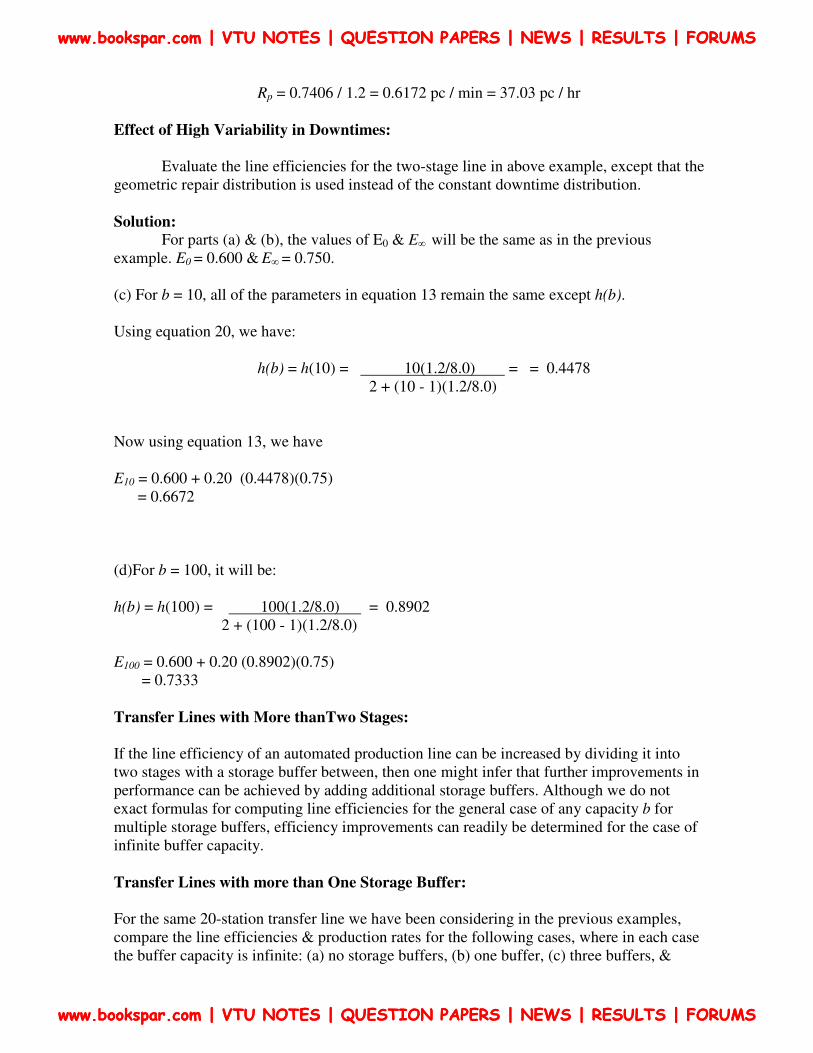
Rp = 0.7406 / 1.2 = 0.6172 pc / min = 37.03 pc / hr Effect of High Variability in Downtimes:

Evaluate the line efficiencies for the two-stage line in above example, except that the geometric repair distribution is used instead of the constant downtime distribution. Solution:

For parts (a) & (b), the values of E0 & E∞ will be the same as in the previous example. E0 = 0.600 & E∞ = 0.750. (c) For b = 10, all of the parameters in equation 13 remain the same except h(b). Using equation 20, we have:

h(b) = h(10) = 10(1.2/8.0) = = 0.4478 2 + (10 - 1)(1.2/8.0)

Now using equation 13, we have E10 = 0.600 + 0.20 (0.4478)(0.75) = 0.6672 (d)For b = 100, it will be: h(b) = h(100) = 100(1.2/8.0) = 0.8902 2 + (100 - 1)(1.2/8.0) E100 = 0.600 + 0.20 (0.8902)(0.75) = 0.7333 Transfer Lines with More thanTwo Stages:

If the line efficiency of an automated production line can be increased by dividing it into two stages with a storage buffer between, then one might infer that further improvements in performance can be achieved by adding additional storage buffers. Although we do not exact formulas for computing line efficiencies for the general case of any capacity b for multiple storage buffers, efficiency improvements can readily be determined for the case of infinite buffer capacity.

Transfer Lines with more than One Storage Buffer:

For the same 20-station transfer line we have been considering in the previous examples, compare the line efficiencies & production rates for the following cases, where in each case the buffer capacity is infinite: (a) no storage buffers, (b) one buffer, (c) three buffers, &





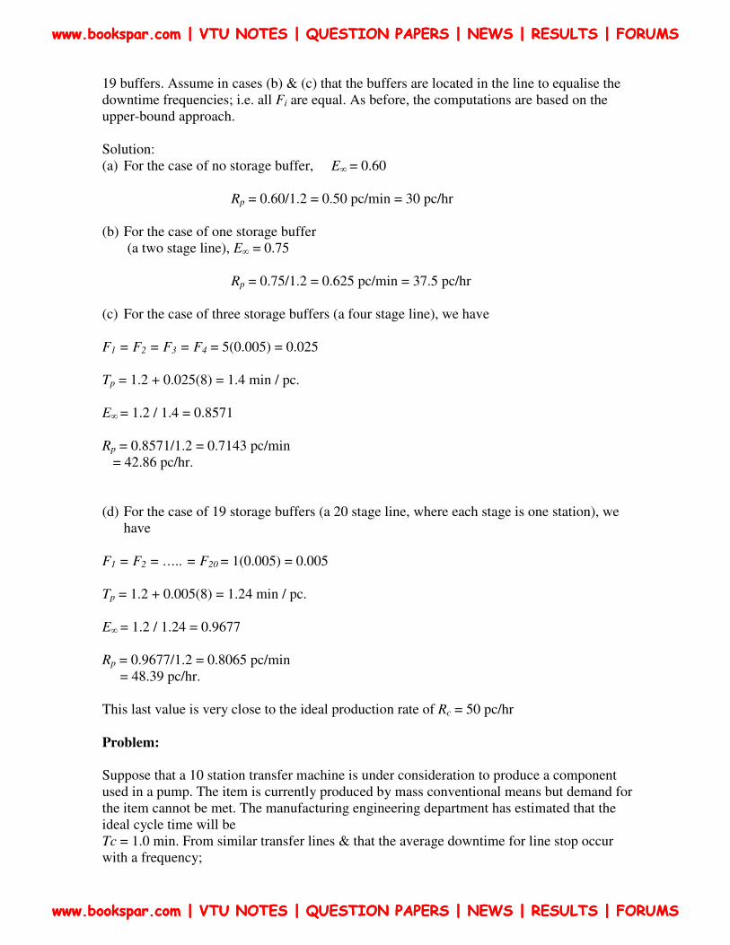
19 buffers. Assume in cases (b) & (c) that the buffers are located in the line to equalise the downtime frequencies; i.e. all Fi are equal. As before, the computations are based on the upper-bound approach. Solution: (a) For the case of no storage buffer, E∞ = 0.60

Rp = 0.60/1.2 = 0.50 pc/min = 30 pc/hr (b) For the case of one storage buffer

(a two stage line), E∞ = 0.75

Rp = 0.75/1.2 = 0.625 pc/min = 37.5 pc/hr (c) For the case of three storage buffers (a four stage line), we have F1 = F2 = F3 = F4 = 5(0.005) = 0.025

Tp = 1.2 + 0.025(8) = 1.4 min / pc.

E∞ = 1.2 / 1.4 = 0.8571

Rp = 0.8571/1.2 = 0.7143 pc/min = 42.86 pc/hr. (d) For the case of 19 storage buffers (a 20 stage line, where each stage is one station), we

have

F1 = F2 = ….. = F20 = 1(0.005) = 0.005 Tp = 1.2 + 0.005(8) = 1.24 min / pc.

E∞ = 1.2 / 1.24 = 0.9677

Rp = 0.9677/1.2 = 0.8065 pc/min = 48.39 pc/hr. This last value is very close to the ideal production rate of Rc = 50 pc/hr Problem:

Suppose that a 10 station transfer machine is under consideration to produce a component used in a pump. The item is currently produced by mass conventional means but demand for the item cannot be met. The manufacturing engineering department has estimated that the ideal cycle time will be Tc = 1.0 min. From similar transfer lines & that the average downtime for line stop occur with a frequency;





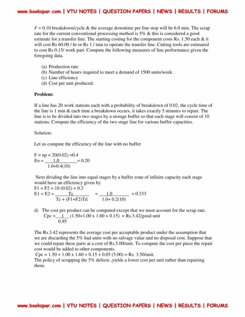
F = 0.10 breakdown/cycle & the average downtime per line stop will be 6.0 min. The scrap rate for the current conventional processing method is 5% & this is considered a good estimate for a transfer line. The starting costing for the component costs Rs. 1.50 each & it will cost Rs 60.00 / hr or Rs 1 / min to operate the transfer line. Cutting tools are estimated to cost Rs 0.15/ work part. Compute the following measures of line performance given the foregoing data.

(a) Production rate (b) Number of hours required to meet a demand of 1500 units/week. (c) Line efficiency (d) Cost per unit produced.

Problem:

If a line has 20 work stations each with a probability of breakdown of 0.02, the cycle time of the line is 1 min & each time a breakdown occurs, it takes exactly 5 minutes to repair. The line is to be divided into two stages by a storage buffer so that each stage will consist of 10 stations. Compute the efficiency of the two stage line for various buffer capacities. Solution: Let us compute the efficiency of the line with no buffer F = np = 20(0.02) =0.4 Eo = 1.0 = 0.20 1.0+0.4(10) Next dividing the line into equal stages by a buffer zone of infinite capacity each stage would have an efficiency given by F1 = F2 = 10 (0.02) = 0.2 E1 = E2 = Tc = 1.0 = 0.333 Tc + (F1+F2)Td 1.0+ 0.2(10) d) The cost per product can be computed except that we must account for the scrap rate. Cpc = 1 (1.50+1.00 x 1.60 + 0.15) = Rs.3.42/good unit 0.95 The Rs.3.42 represents the average cost per acceptable product under the assumption that we are discarding the 5% bad units with no salvage value and no disposal cost. Suppose that we could repair these parts at a cost of Rs.5.00/unit. To compute the cost per piece the repair cost would be added to other components. Cpc = 1.50 + 1.00 x 1.60 + 0.15 + 0.05 (5.00) = Rs. 3.50/unit. The policy of scrapping the 5% defects ,yields a lower cost per unit rather than repairing them.





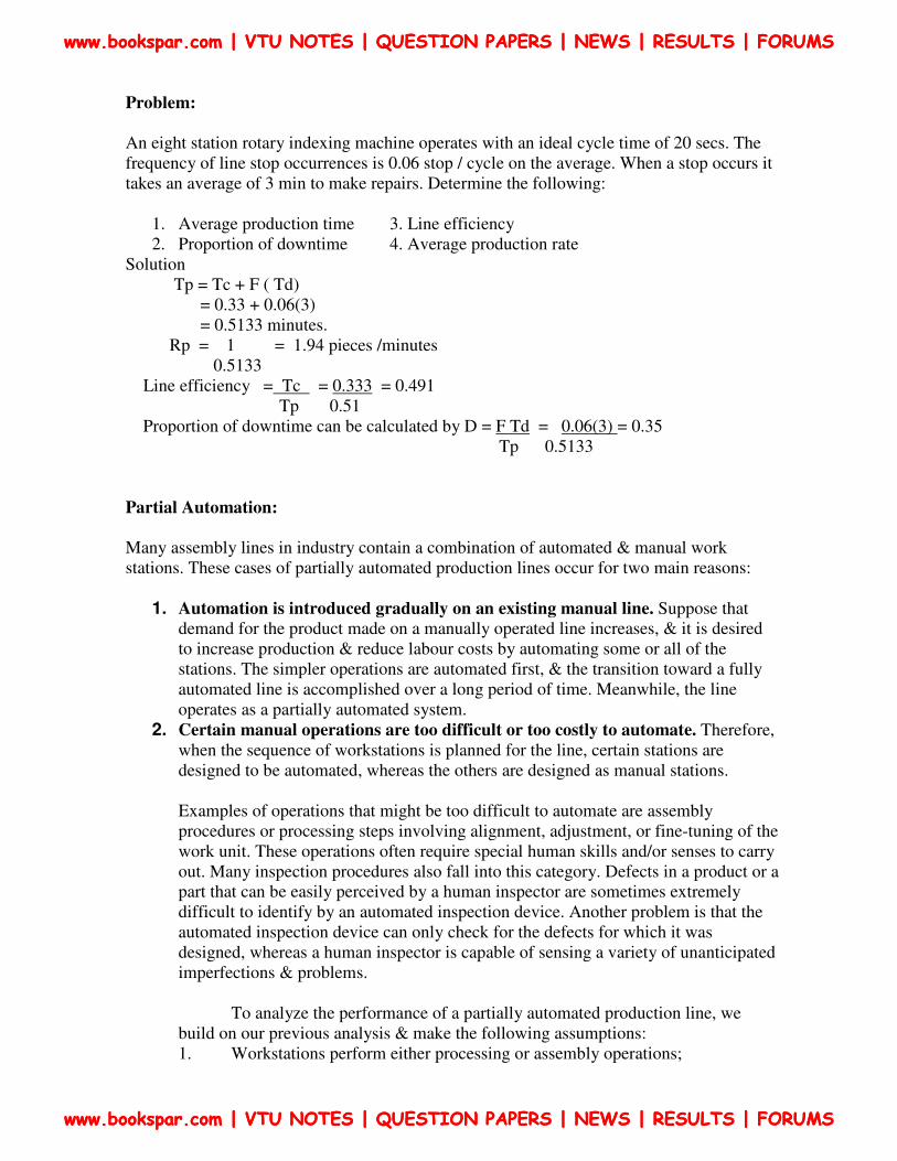
Problem:

An eight station rotary indexing machine operates with an ideal cycle time of 20 secs. The frequency of line stop occurrences is 0.06 stop / cycle on the average. When a stop occurs it takes an average of 3 min to make repairs. Determine the following:

1. Average production time 3. Line efficiency 2. Proportion of downtime 4. Average production rate

Solution Tp = Tc + F ( Td) = 0.33 + 0.06(3) = 0.5133 minutes. Rp = 1 = 1.94 pieces /minutes 0.5133 Line efficiency = Tc = 0.333 = 0.491 Tp 0.51 Proportion of downtime can be calculated by D = F Td = 0.06(3) = 0.35 Tp 0.5133 Partial Automation:

Many assembly lines in industry contain a combination of automated & manual work stations. These cases of partially automated production lines occur for two main reasons:

1. Automation is introduced gradually on an existing manual line. Suppose that demand for the product made on a manually operated line increases, & it is desired to increase production & reduce labour costs by automating some or all of the stations. The simpler operations are automated first, & the transition toward a fully automated line is accomplished over a long period of time. Meanwhile, the line operates as a partially automated system.

2. Certain manual operations are too difficult or too costly to automate. Therefore, when the sequence of workstations is planned for the line, certain stations are designed to be automated, whereas the others are designed as manual stations. Examples of operations that might be too difficult to automate are assembly procedures or processing steps involving alignment, adjustment, or fine-tuning of the work unit. These operations often require special human skills and/or senses to carry out. Many inspection procedures also fall into this category. Defects in a product or a part that can be easily perceived by a human inspector are sometimes extremely difficult to identify by an automated inspection device. Another problem is that the automated inspection device can only check for the defects for which it was designed, whereas a human inspector is capable of sensing a variety of unanticipated imperfections & problems. To analyze the performance of a partially automated production line, we build on our previous analysis & make the following assumptions: 1. Workstations perform either processing or assembly operations;





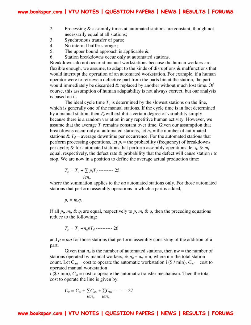
2. Processing & assembly times at automated stations are constant, though not necessarily equal at all stations;

3. Synchronous transfer of parts; 4. No internal buffer storage ; 5. The upper bound approach is applicable & 6. Station breakdowns occur only at automated stations. Breakdowns do not occur at manual workstations because the human workers are flexible enough, we assume, to adapt to the kinds of disruptions & malfunctions that would interrupt the operation of an automated workstation. For example, if a human operator were to retrieve a defective part from the parts bin at the station, the part would immediately be discarded & replaced by another without much lost time. Of course, this assumption of human adaptability is not always correct, but our analysis is based on it. The ideal cycle time Tc is determined by the slowest stations on the line, which is generally one of the manual stations. If the cycle time is in fact determined by a manual station, then Tc will exhibit a certain degree of variability simply because there is a random variation in any repetitive human activity. However, we assume that the average Tc remains constant over time. Given our assumption that breakdowns occur only at automated stations, let na = the number of automated stations & Td = average downtime per occurrence. For the automated stations that perform processing operations, let pi = the probability (frequency) of breakdowns per cycle; & for automated stations that perform assembly operations, let qi & mi equal, respectively, the defect rate & probability that the defect will cause station i to stop. We are now in a position to define the average actual production time: Tp = Tc + ∑ piTd --------- 25

iєna

where the summation applies to the na automated stations only. For those automated stations that perform assembly operations in which a part is added, pi = miqi

If all pi, mi, & qi are equal, respectively to p, m, & q, then the preceding equations reduce to the following: Tp = Tc +napTd ---------- 26 and p = mq for those stations that perform assembly consisting of the addition of a part. Given that na is the number of automated stations, then nw = the number of stations operated by manual workers, & na + nw = n, where n = the total station count. Let Casi = cost to operate the automatic workstation i ($ / min), Cwi = cost to operated manual workstation i ($ / min), Cat = cost to operate the automatic transfer mechanism. Then the total cost to operate the line is given by: Co = Cat + ∑Casi + ∑Cwi -------- 27 iєna iєnw





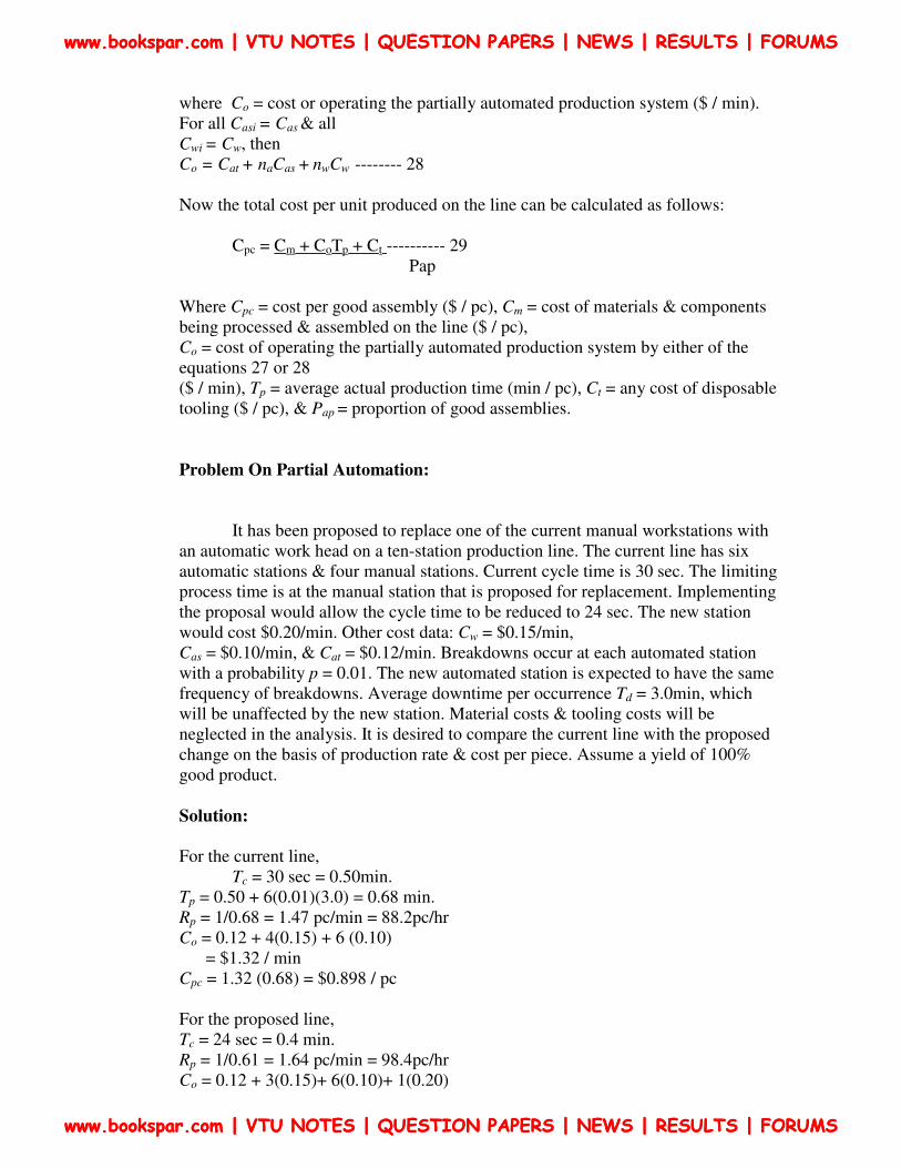
where Co = cost or operating the partially automated production system ($ / min). For all Casi = Cas & all Cwi = Cw, then Co = Cat + naCas + nwCw -------- 28 Now the total cost per unit produced on the line can be calculated as follows: Cpc = Cm + CoTp + Ct ---------- 29 Pap Where Cpc = cost per good assembly ($ / pc), Cm = cost of materials & components being processed & assembled on the line ($ / pc), Co = cost of operating the partially automated production system by either of the equations 27 or 28 ($ / min), Tp = average actual production time (min / pc), Ct = any cost of disposable tooling ($ / pc), & Pap = proportion of good assemblies.

Problem On Partial Automation:

It has been proposed to replace one of the current manual workstations with an automatic work head on a ten-station production line. The current line has six automatic stations & four manual stations. Current cycle time is 30 sec. The limiting process time is at the manual station that is proposed for replacement. Implementing the proposal would allow the cycle time to be reduced to 24 sec. The new station would cost $0.20/min. Other cost data: Cw = $0.15/min, Cas = $0.10/min, & Cat = $0.12/min. Breakdowns occur at each automated station with a probability p = 0.01. The new automated station is expected to have the same frequency of breakdowns. Average downtime per occurrence Td = 3.0min, which will be unaffected by the new station. Material costs & tooling costs will be neglected in the analysis. It is desired to compare the current line with the proposed change on the basis of production rate & cost per piece. Assume a yield of 100% good product. Solution:

For the current line,

Tc = 30 sec = 0.50min. Tp = 0.50 + 6(0.01)(3.0) = 0.68 min. Rp = 1/0.68 = 1.47 pc/min = 88.2pc/hr Co = 0.12 + 4(0.15) + 6 (0.10) = $1.32 / min Cpc = 1.32 (0.68) = $0.898 / pc For the proposed line, Tc = 24 sec = 0.4 min. Rp = 1/0.61 = 1.64 pc/min = 98.4pc/hr Co = 0.12 + 3(0.15)+ 6(0.10)+ 1(0.20)





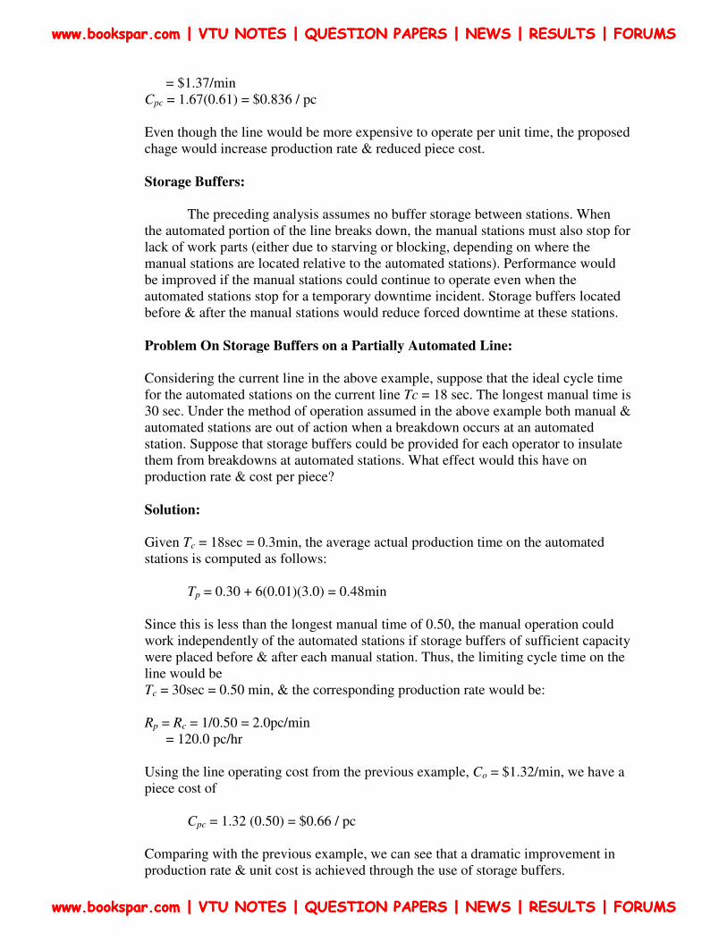
= $1.37/min Cpc = 1.67(0.61) = $0.836 / pc Even though the line would be more expensive to operate per unit time, the proposed chage would increase production rate & reduced piece cost. Storage Buffers:

The preceding analysis assumes no buffer storage between stations. When the automated portion of the line breaks down, the manual stations must also stop for lack of work parts (either due to starving or blocking, depending on where the manual stations are located relative to the automated stations). Performance would be improved if the manual stations could continue to operate even when the automated stations stop for a temporary downtime incident. Storage buffers located before & after the manual stations would reduce forced downtime at these stations. Problem On Storage Buffers on a Partially Automated Line:

Considering the current line in the above example, suppose that the ideal cycle time for the automated stations on the current line Tc = 18 sec. The longest manual time is 30 sec. Under the method of operation assumed in the above example both manual & automated stations are out of action when a breakdown occurs at an automated station. Suppose that storage buffers could be provided for each operator to insulate them from breakdowns at automated stations. What effect would this have on production rate & cost per piece? Solution:

Given Tc = 18sec = 0.3min, the average actual production time on the automated stations is computed as follows: Tp = 0.30 + 6(0.01)(3.0) = 0.48min Since this is less than the longest manual time of 0.50, the manual operation could work independently of the automated stations if storage buffers of sufficient capacity were placed before & after each manual station. Thus, the limiting cycle time on the line would be Tc = 30sec = 0.50 min, & the corresponding production rate would be: Rp = Rc = 1/0.50 = 2.0pc/min = 120.0 pc/hr Using the line operating cost from the previous example, Co = $1.32/min, we have a piece cost of Cpc = 1.32 (0.50) = $0.66 / pc Comparing with the previous example, we can see that a dramatic improvement in production rate & unit cost is achieved through the use of storage buffers.





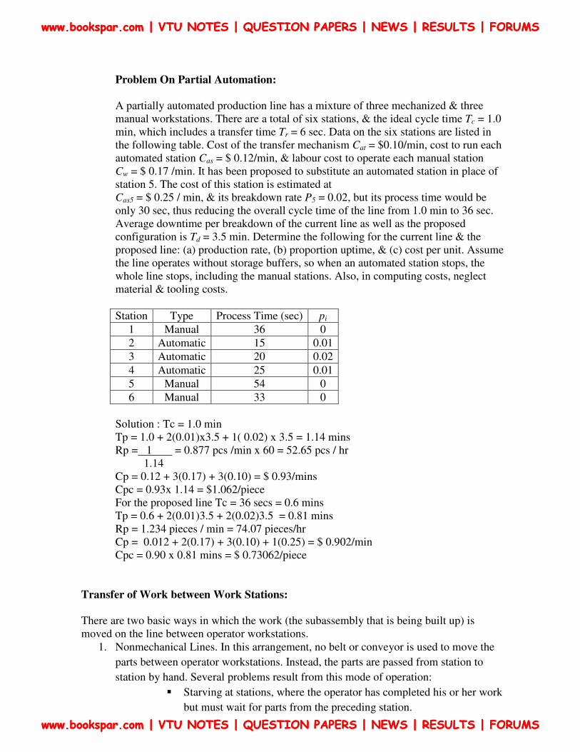
Problem On Partial Automation:

A partially automated production line has a mixture of three mechanized & three manual workstations. There are a total of six stations, & the ideal cycle time Tc = 1.0 min, which includes a transfer time Tr = 6 sec. Data on the six stations are listed in the following table. Cost of the transfer mechanism Cat = $0.10/min, cost to run each automated station Cas = $ 0.12/min, & labour cost to operate each manual station Cw = $ 0.17 /min. It has been proposed to substitute an automated station in place of station 5. The cost of this station is estimated at Cas5 = $ 0.25 / min, & its breakdown rate P5 = 0.02, but its process time would be only 30 sec, thus reducing the overall cycle time of the line from 1.0 min to 36 sec. Average downtime per breakdown of the current line as well as the proposed configuration is Td = 3.5 min. Determine the following for the current line & the proposed line: (a) production rate, (b) proportion uptime, & (c) cost per unit. Assume the line operates without storage buffers, so when an automated station stops, the whole line stops, including the manual stations. Also, in computing costs, neglect material & tooling costs.

Station Type Process Time (sec) pi

1 Manual 36 0

2 Automatic 15 0.01

3 Automatic 20 0.02

4 Automatic 25 0.01

5 Manual 54 0

6 Manual 33 0

Solution : Tc = 1.0 min Tp = 1.0 + 2(0.01)x3.5 + 1( 0.02) x 3.5 = 1.14 mins Rp = 1 = 0.877 pcs /min x 60 = 52.65 pcs / hr 1.14 Cp = 0.12 + 3(0.17) + 3(0.10) = $ 0.93/mins Cpc = 0.93x 1.14 = $1.062/piece For the proposed line Tc = 36 secs = 0.6 mins Tp = 0.6 + 2(0.01)3.5 + 2(0.02)3.5 = 0.81 mins Rp = 1.234 pieces / min = 74.07 pieces/hr Cp = 0.012 + 2(0.17) + 3(0.10) + 1(0.25) = $ 0.902/min Cpc = 0.90 x 0.81 mins = $ 0.73062/piece

Transfer of Work between Work Stations:

There are two basic ways in which the work (the subassembly that is being built up) is moved on the line between operator workstations.

1. Nonmechanical Lines. In this arrangement, no belt or conveyor is used to move the

parts between operator workstations. Instead, the parts are passed from station to

station by hand. Several problems result from this mode of operation:

� Starving at stations, where the operator has completed his or her work

but must wait for parts from the preceding station.





� Blocking of stations, where the operator has completed his or her

work but must wait for the next operator to finish the task before

passing along the part.

As a result of these problems, the flow of work on a nonmechanical line is usually uneven. The cycle times vary, and this contributes to the overall irregularity. Buffer stocks of parts between workstations are often used to smooth out the production flow.

• Moving conveyor lines. These flow lines use a conveyor (e.g., a moving belt,

conveyor, chain-in-the-floor, etc.) to move the subassemblies between workstations.

The transport system can be continuous, intermittent (synchronous), or

asynchronous. Continuous transfer is most common in assembly lines, although

asynchronous transfer is becoming more popular. With the continuously moving

conveyor, the following problems can arise:

� Starving can occur as with non mechanical lines.

� Incomplete items are sometimes produced when the operator is

unable to finish the current part & the next part travels right by on the

conveyor. Blocking does not occur.

Again, buffer stocks are sometimes used to overcome these problems. Also stations overlaps can sometimes be allowed, where the worker is permitted to travel beyond the normal boundaries of the station in order to complete work.

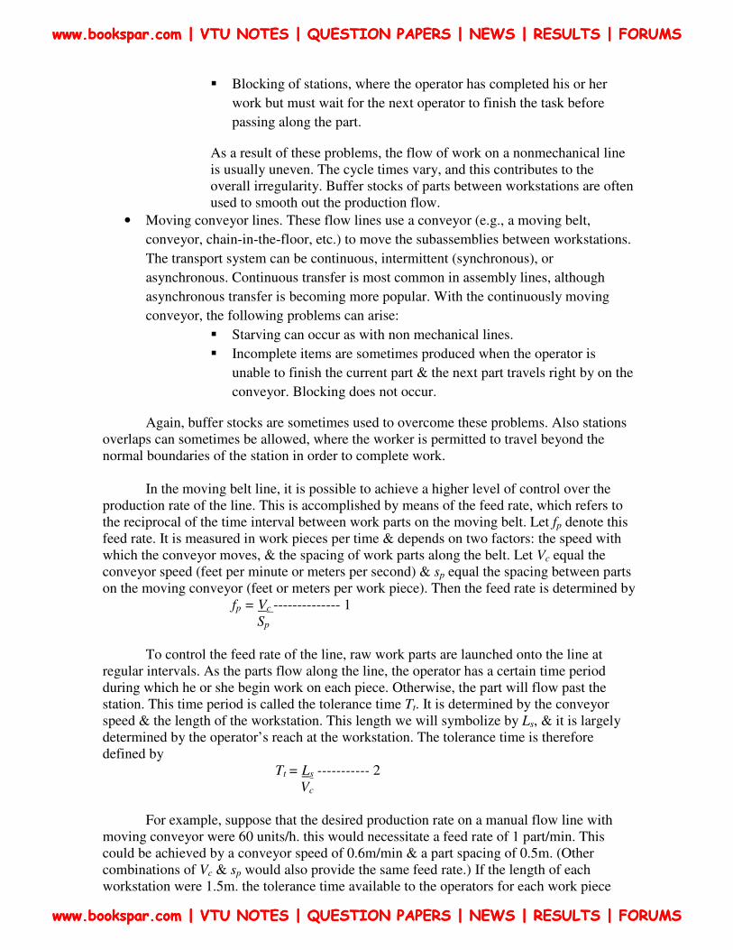
In the moving belt line, it is possible to achieve a higher level of control over the production rate of the line. This is accomplished by means of the feed rate, which refers to the reciprocal of the time interval between work parts on the moving belt. Let fp denote this feed rate. It is measured in work pieces per time & depends on two factors: the speed with which the conveyor moves, & the spacing of work parts along the belt. Let Vc equal the conveyor speed (feet per minute or meters per second) & sp equal the spacing between parts on the moving conveyor (feet or meters per work piece). Then the feed rate is determined by fp = Vc -------------- 1 Sp

To control the feed rate of the line, raw work parts are launched onto the line at regular intervals. As the parts flow along the line, the operator has a certain time period during which he or she begin work on each piece. Otherwise, the part will flow past the station. This time period is called the tolerance time Tt. It is determined by the conveyor speed & the length of the workstation. This length we will symbolize by Ls, & it is largely determined by the operator’s reach at the workstation. The tolerance time is therefore defined by Tt = Ls ----------- 2 Vc

For example, suppose that the desired production rate on a manual flow line with

moving conveyor were 60 units/h. this would necessitate a feed rate of 1 part/min. This could be achieved by a conveyor speed of 0.6m/min & a part spacing of 0.5m. (Other combinations of Vc & sp would also provide the same feed rate.) If the length of each workstation were 1.5m. the tolerance time available to the operators for each work piece





would be 3 min. It is generally desirable to make the tolerance time large to compensate for worker process time variability.

Mode Variations:

In both nonmechanical lines & moving conveyor lines it is highly desirable to assign

work to the stations so as to equalize the process or assembly times at the workstations. The problem is sometimes complicated by the fact that the same production line may be called upon to process more than one type of product. This complication gives rise to the identification of three flow line cases (and therefore three different types of line balancing problems). The three production situations on flow lines are defined according to the product or products to be made on the line. Will the flow line be used exclusively to produce one particular model? Or, will it be used to produce several different models, & if so how will they be scheduled on line? There are three cases that can be defined in response to these questions:

1. Single-model line. This is a specialized line dedicated to the production of a single model or product. The demand rate for the product is great enough that the line is devoted 100% of the time to the production of that product.

2. Batch-model line. This line is used for the production of two or more models. Each model is produced in batches on the line. The models or products are usually similar in the sense of requiring a similar sequence of processing or assembly operations. It is for this reason that the same line can be used to produce the various models.

3. Mixed-model lines. This line is also used for the production of two or more models, but the various models are intermixed on the line so that several different models are being produced simultaneously rather than in batches. Automobile & truck assembly lines are examples of this case.

To gain a better perspective of the three cases, the reader might consider the following. In the case of the batch-model line, if the batch sizes are very large, the batch-model line approaches the case of the single-model line. If the batch sizes become very small (approaching a batch size of 1), the batch-model line approximates to the case of the mixed-model line.

In principle, the three cases can be applied in both manual flow lines & automated flow lines. However, in practice, the flexibility of human operators makes the latter two cases more feasible on the manual assembly line. It is anticipated that future automated lines will incorporate quick changeover & programming capabilities within their designs to permit the batch-model, & eventually the mixed-model, concepts to become practicable.

Achieving a balanced allocation of work load among stations of the line is a problem in all three cases. The problem is least formidable for the single-model case. For the batch-model line, the balancing problem becomes more difficult; & for the mixed-model case, the problem of line balancing becomes quite complicated.

In this chapter we consider only the single-model line balancing problem, although the same concepts & similar terminology & methodology apply for the batch & mixed model cases.





The Line Balancing Problem:

In flow line production there are many separate & distinct processing & assembly

operations to be performed on the product. Invariably, the sequence of processing or assembly steps is restricted, at least to some extent, in terms of the order in which the operations can be carried out. For example, a threaded hole must be drilled before it can be tapped. In mechanical fastening, the washer must be placed over the bolt before the nut can be turned & tightened. These restrictions are called precedence constraints in the language of line balancing. It is generally the case that the product must be manufactured at some specified production rate in order to satisfy demand for the product. Whether we are concerned with performing these processes & assembly operations on automatic machines or manual flow lines, it is desirable to design the line so as to satisfy all of the foregoing specifications as efficiently as possible.

The line balancing problem is to arrange the individual processing & assembly tasks at the workstations so that the total time required at each workstation is approximately the same. If the work elements can be grouped so that all the station times are exactly equal, we have perfect balance on the line & we can expect the production to flow smoothly. In most practical situations it is very difficult to achieve perfect balance. When the workstations times are unequal, the slowest station determines the overall production rate of the line.

In order to discuss the terminology & relationships in line balancing, we shall refer to the following example. Later, when discussing the various solution techniques, we shall apply the techniques to this problem.





Documents

UNIT 3: ANALYSIS OF AUTOMATED FLOW LINE & LINE · PDF file · 2013-03-31ANALYSIS OF AUTOMATED FLOW LINE & LINE BALANCING ... Process Technology refers to the body of knowledge about