Unit 2 ppt2

8/13/2019 Unit 2 ppt2

http://slidepdf.com/reader/full/unit-2-ppt2 1/29

Noise Models and Filtering

8/13/2019 Unit 2 ppt2


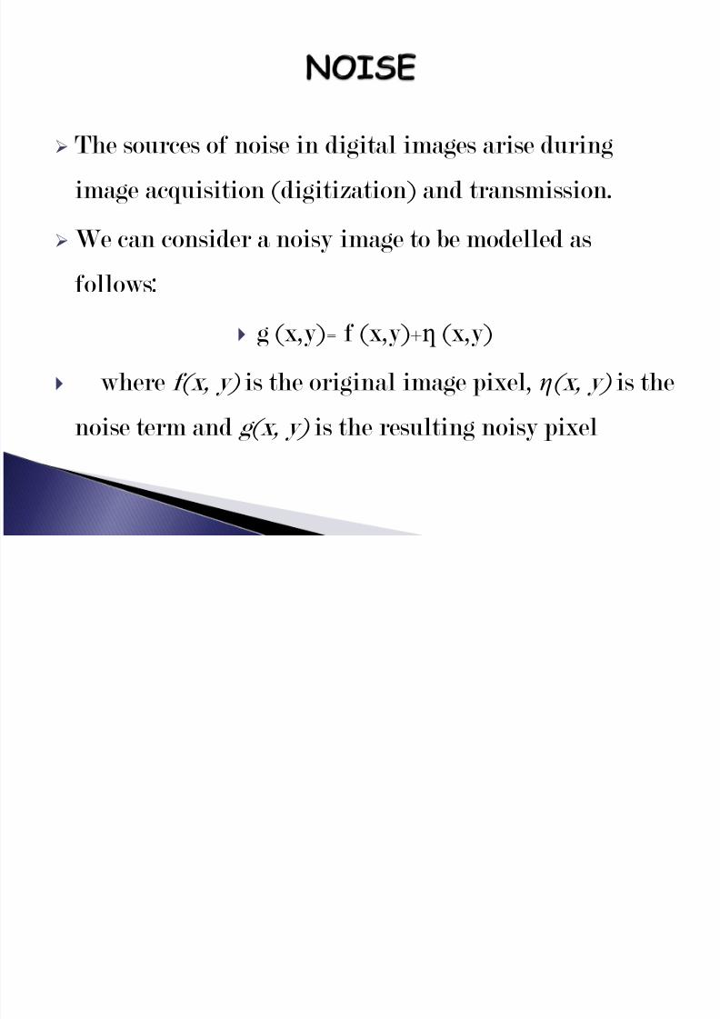
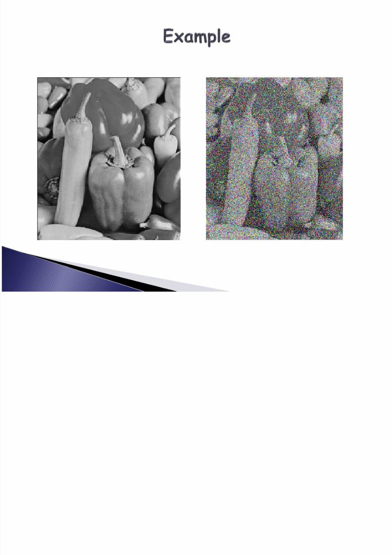
The sources of noise in digital images arise during

image acquisition (digitization) and transmission.

We can consider a noisy image to be modelled asfollows:

g (x,y)= f (x,y)+ ƞ (x,y)

where f(x, y) is the original image pixel, η (x, y) is the

noise term and g(x, y) is the resulting noisy pixel

8/13/2019 Unit 2 ppt2


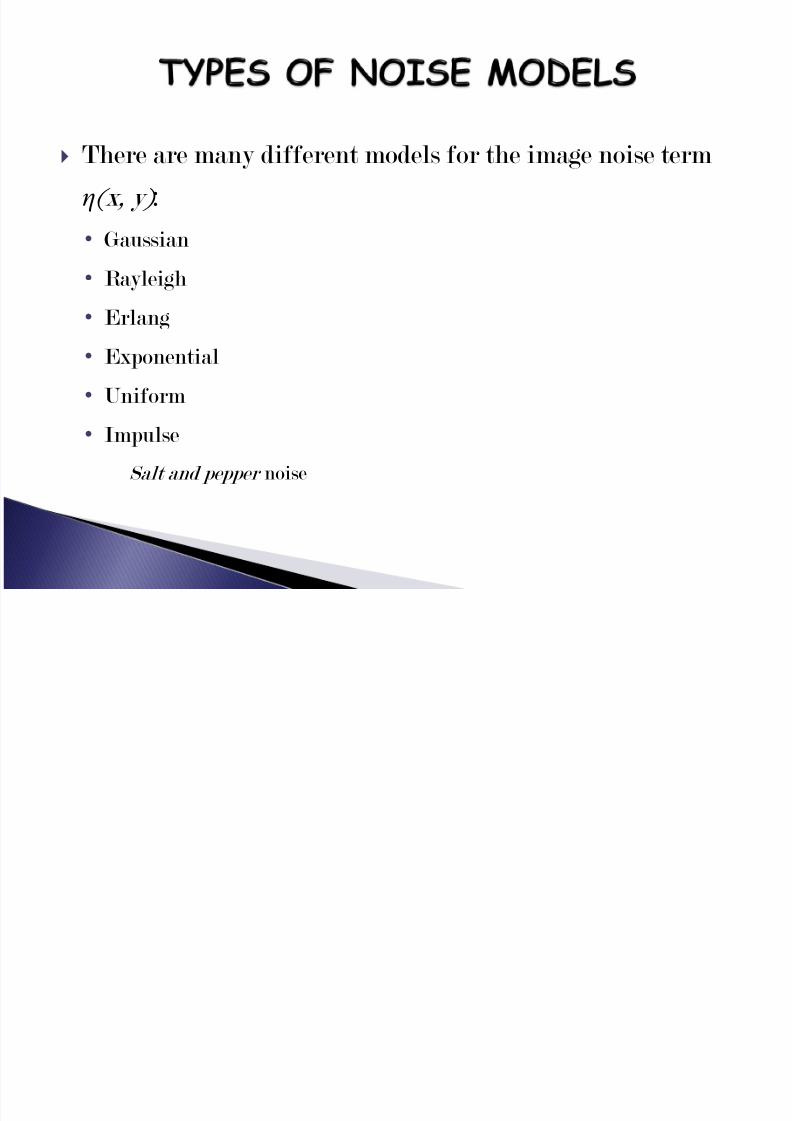
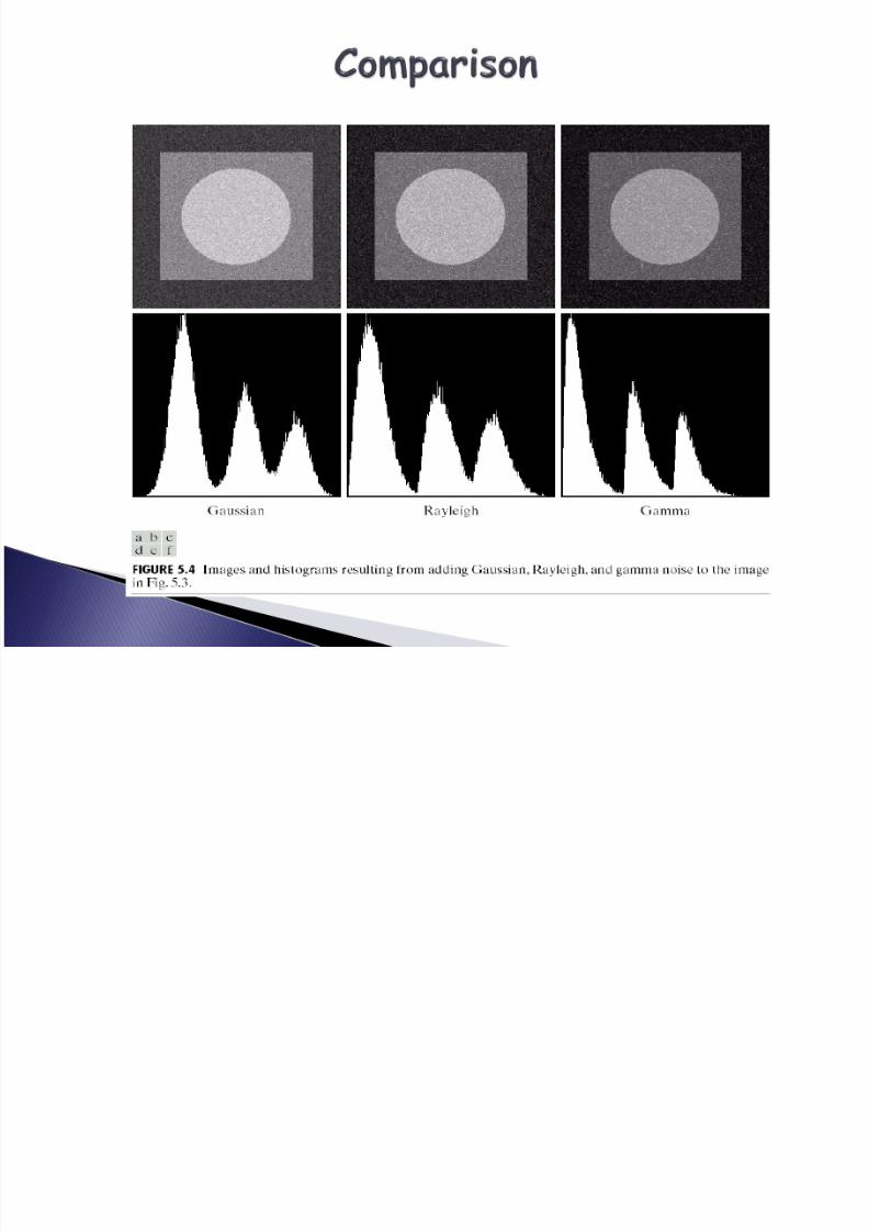
There are many different models for the image noise term

η (x, y) :• Gaussian

• Rayleigh• Erlang• Exponential• Uniform• Impulse

Salt and pepper noise

8/13/2019 Unit 2 ppt2


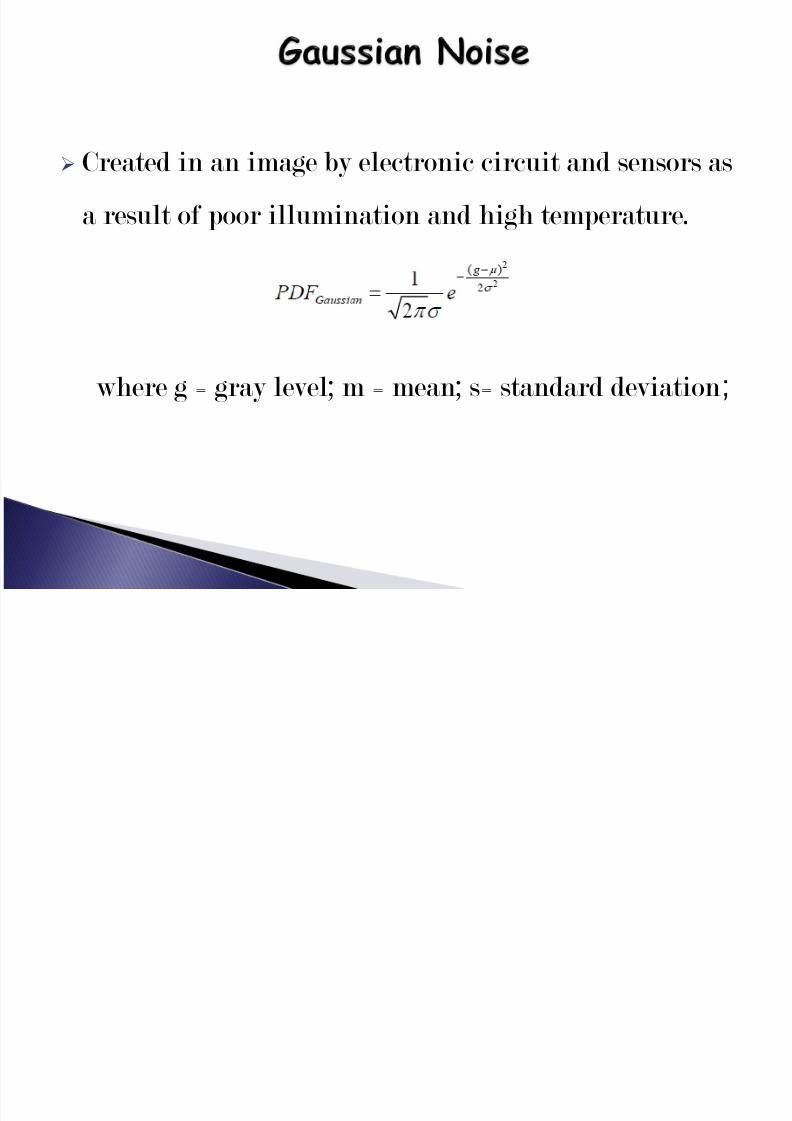
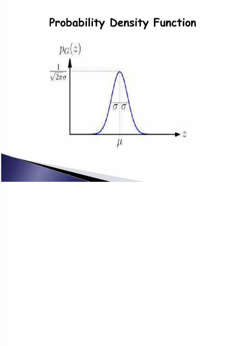
Created in an image by electronic circuit and sensors as

a result of poor illumination and high temperature.

where g = gray level; m = mean; s= standard deviation ;

8/13/2019 Unit 2 ppt2


8/13/2019 Unit 2 ppt2


8/13/2019 Unit 2 ppt2


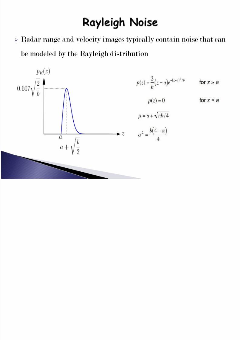
Radar range and velocity images typically contain noise that can be modeled by the Rayleigh distribution

8/13/2019 Unit 2 ppt2


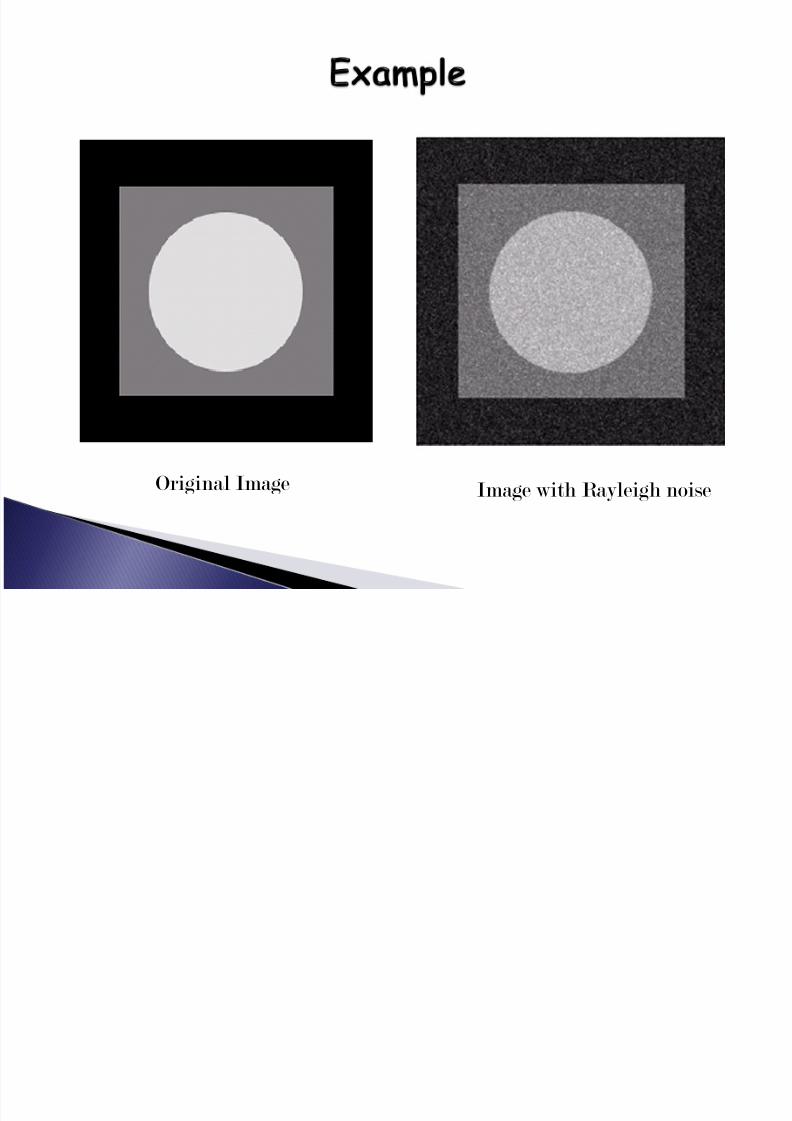
Original Image Image with Rayleigh noise

8/13/2019 Unit 2 ppt2


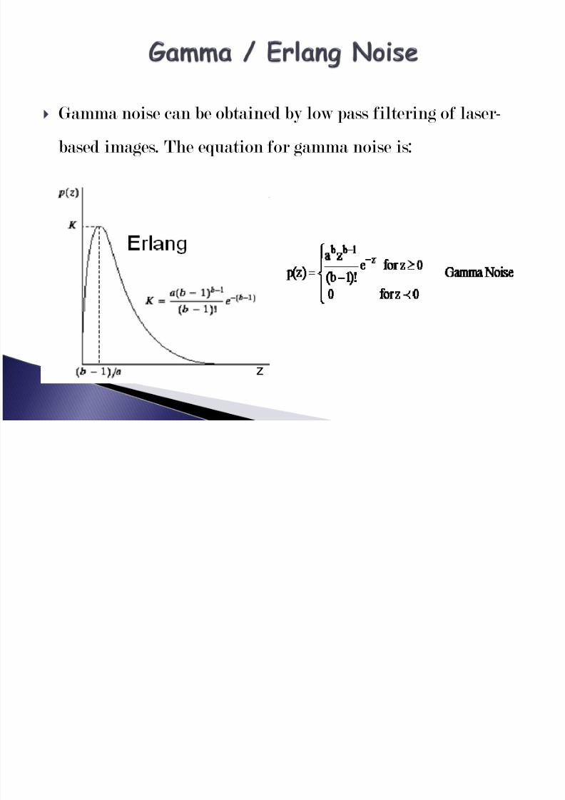
Gamma noise can be obtained by low pass filtering of laser-

based images. The equation for gamma noise is:

z

8/13/2019 Unit 2 ppt2


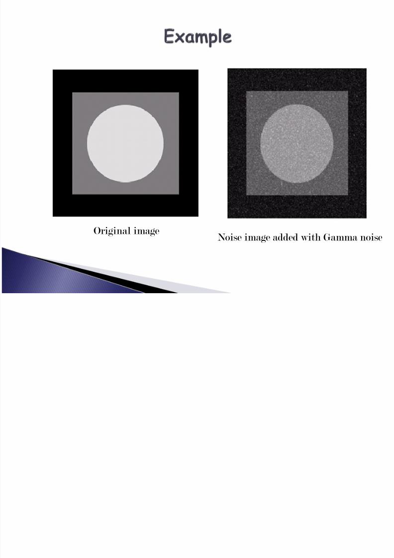
Original imageNoise image added with Gamma noise

8/13/2019 Unit 2 ppt2


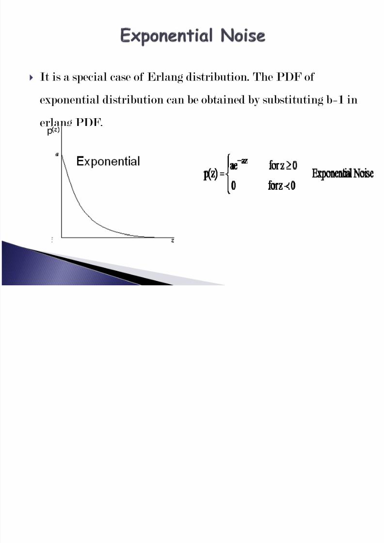
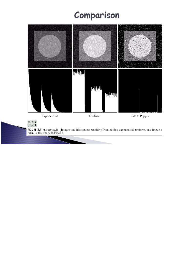
It is a special case of Erlang distribution. The PDF of

exponential distribution can be obtained by substituting b=1 in

erlang PDF.p

8/13/2019 Unit 2 ppt2


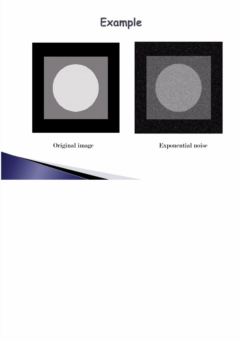
Original image Exponential noise

8/13/2019 Unit 2 ppt2


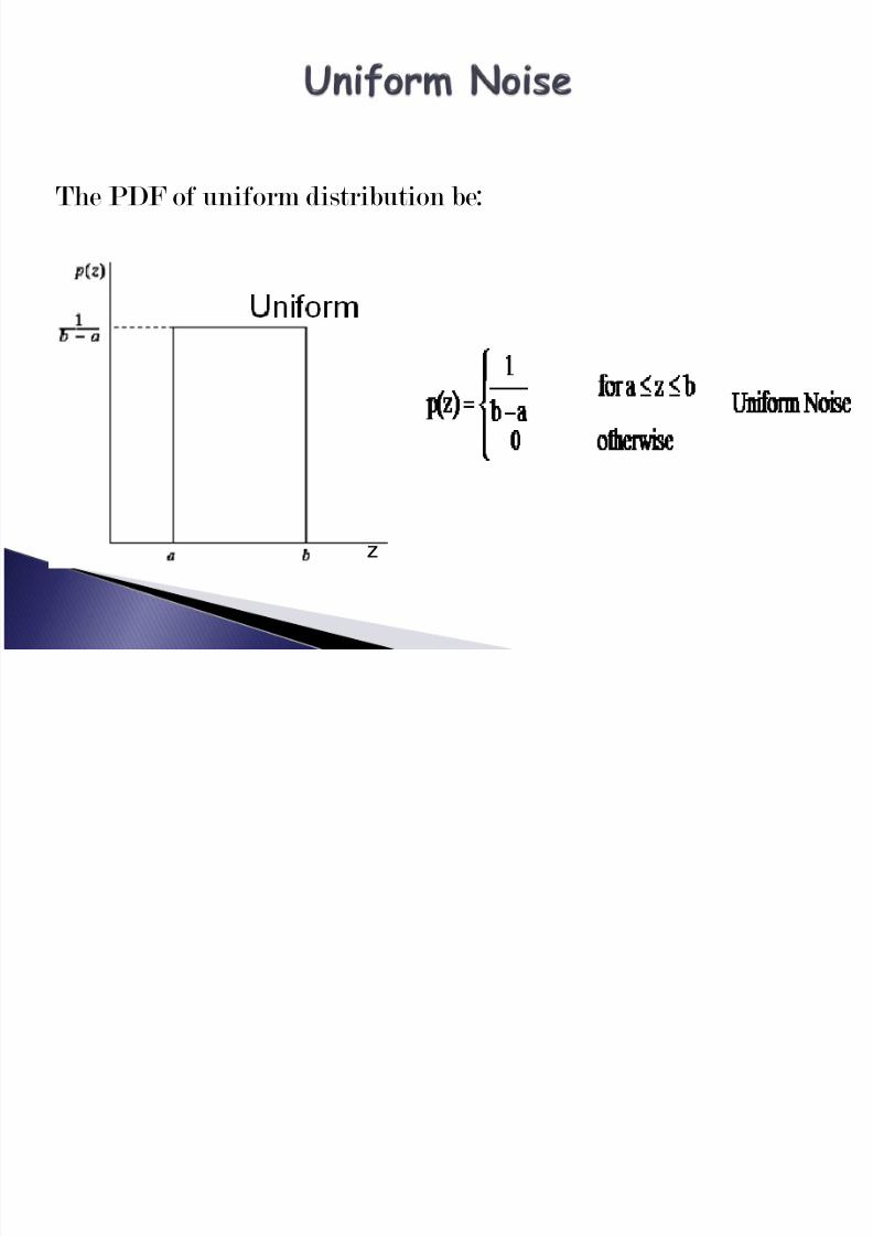
The PDF of uniform distribution be:

z

8/13/2019 Unit 2 ppt2


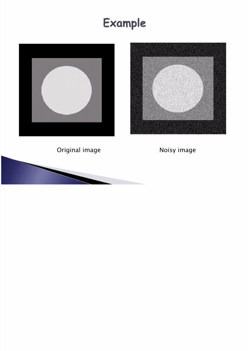
Original image Noisy image

8/13/2019 Unit 2 ppt2


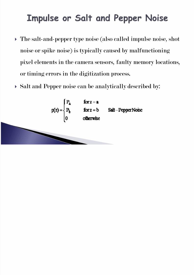
The salt-and-pepper type noise (also called impulse noise, shot

noise or spike noise) is typically caused by malfunctioning

pixel elements in the camera sensors, faulty memory locations,

or timing errors in the digitization process.

Salt and Pepper noise can be analytically described by:

8/13/2019 Unit 2 ppt2


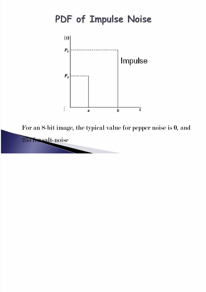
For an 8-bit image, the typical value for pepper noise is 0, and

255 for salt-noise

8/13/2019 Unit 2 ppt2


8/13/2019 Unit 2 ppt2


8/13/2019 Unit 2 ppt2


8/13/2019 Unit 2 ppt2


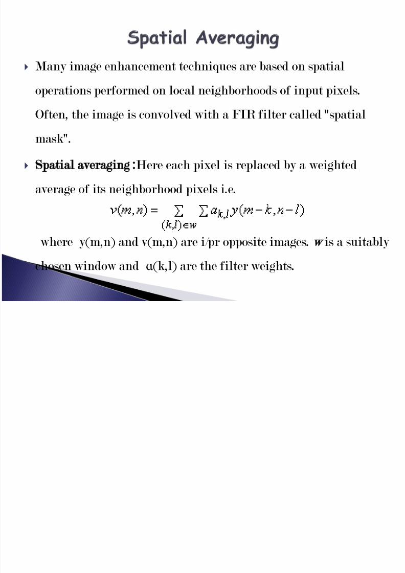
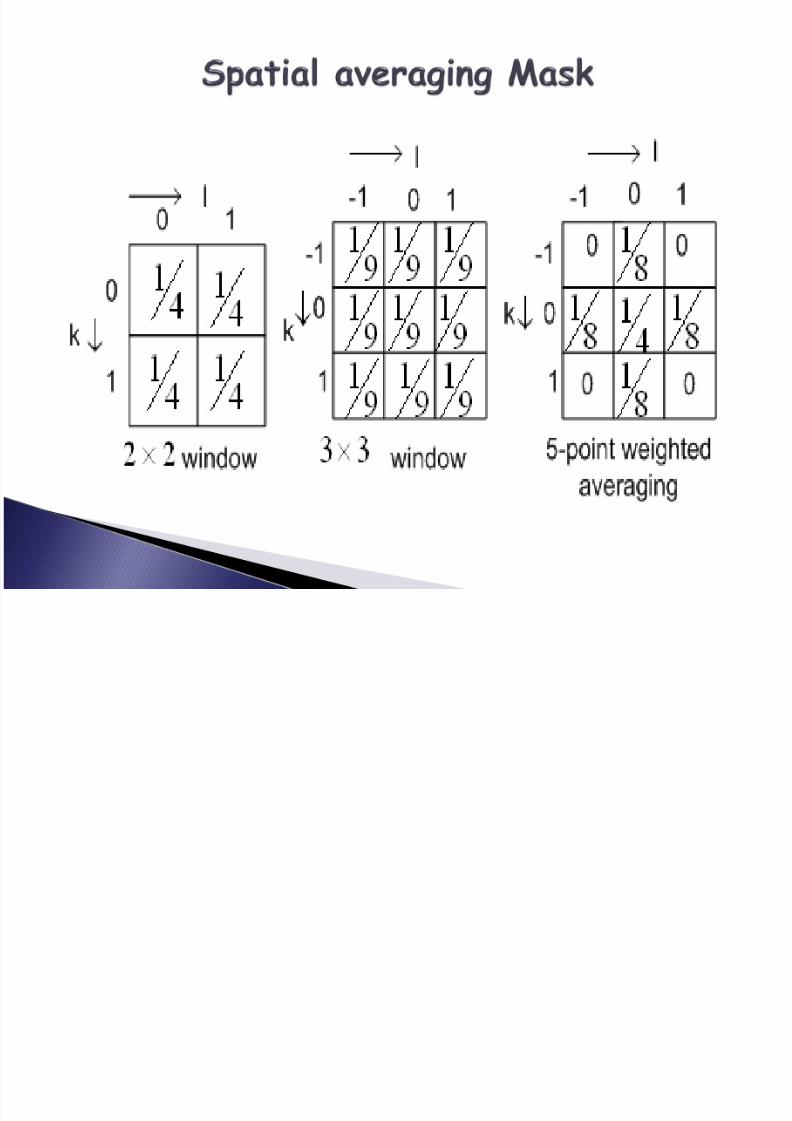
Many image enhancement techniques are based on spatialoperations performed on local neighborhoods of input pixels.

Often, the image is convolved with a FIR filter called "spatial

mask".Spatial averaging Here each pixel is replaced by a weighted

average of its neighborhood pixels i.e.

where y(m,n) and v(m,n) are i/pr opposite images. is a suitably

chosen window and ɑ (k,l) are the filter weights.

8/13/2019 Unit 2 ppt2


8/13/2019 Unit 2 ppt2


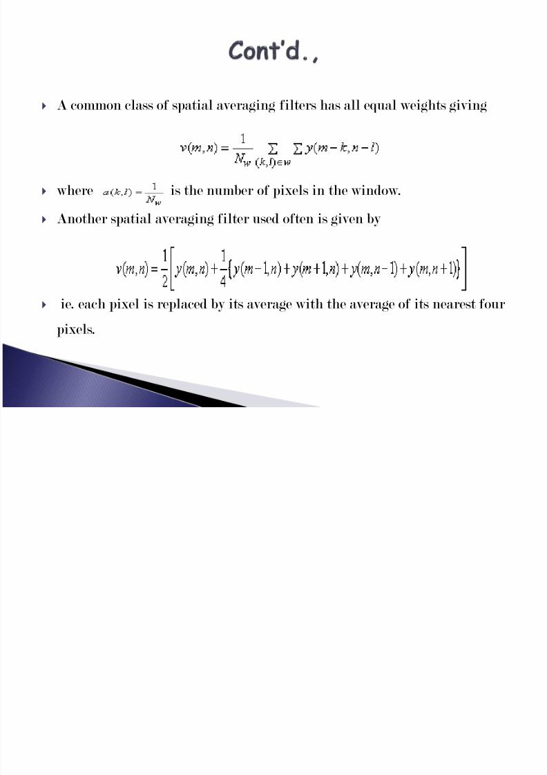
A common class of spatial averaging filters has all equal weights giving

where is the number of pixels in the window.Another spatial averaging filter used often is given by

ie. each pixel is replaced by its average with the average of its nearest four

pixels.

8/13/2019 Unit 2 ppt2


8/13/2019 Unit 2 ppt2


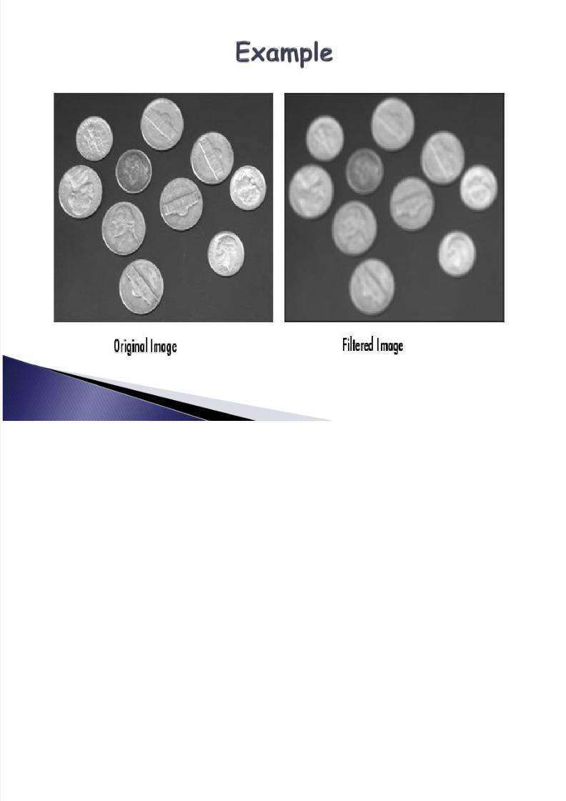
In practice, the pixels are not constant. Hence the window size

is limited. Due to this, the output image of spatial averaging is

distorted in the form of BLURRING.

To protect the edges from blurring while smoothing, a

DIRECTIONAL AVERAGING FILTER is needed. Such a

filtering process is called Directional Smoothing.

8/13/2019 Unit 2 ppt2


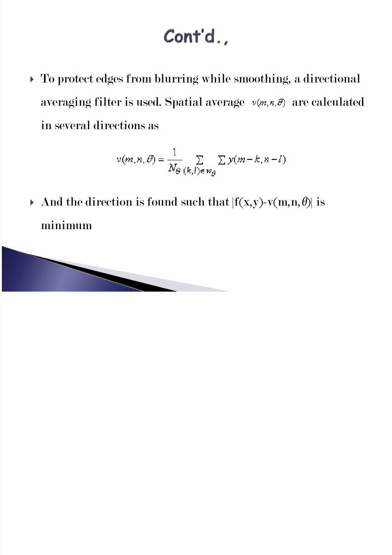
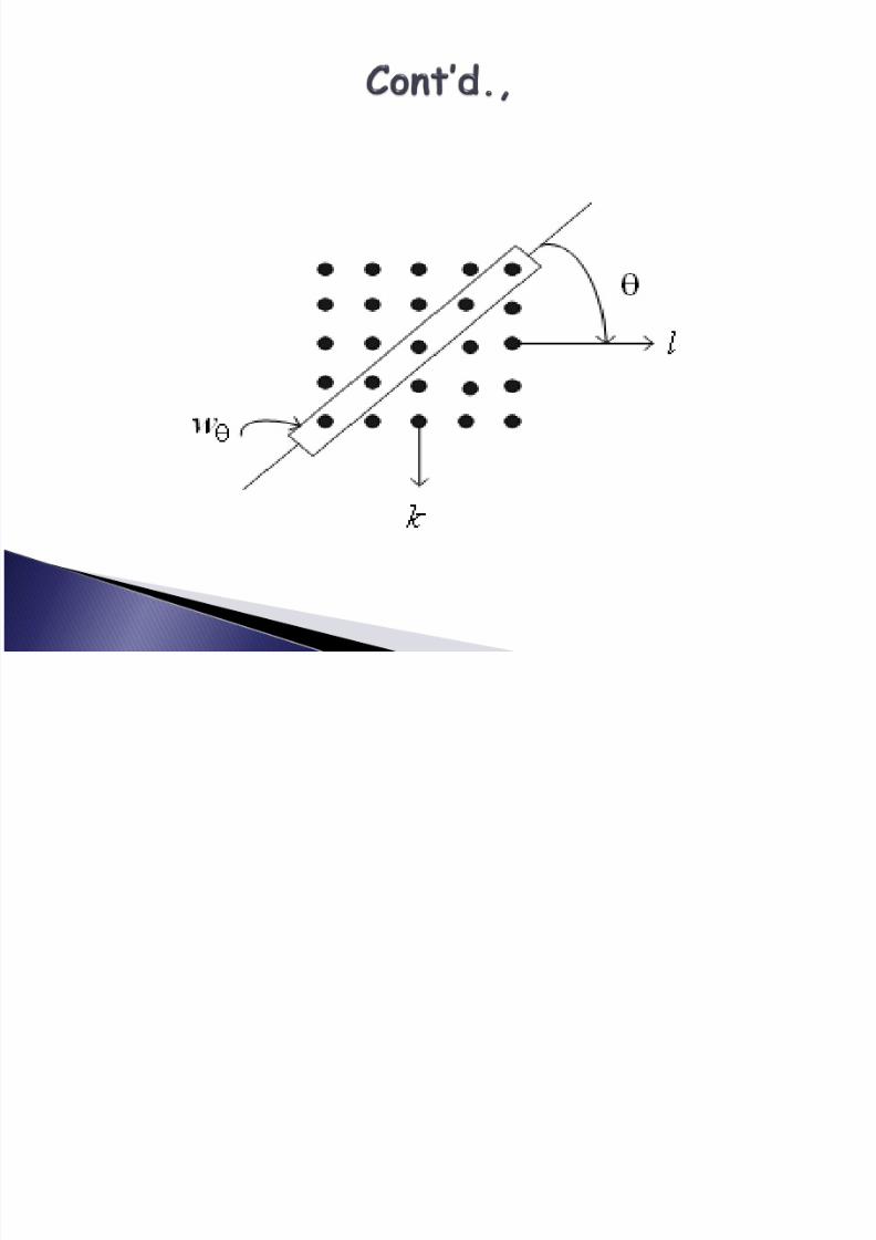
To protect edges from blurring while smoothing, a directional

averaging filter is used. Spatial average are calculated

in several directions as

And the direction is found such that |f(x,y)-v(m,n,θ )| is

minimum

8/13/2019 Unit 2 ppt2


8/13/2019 Unit 2 ppt2


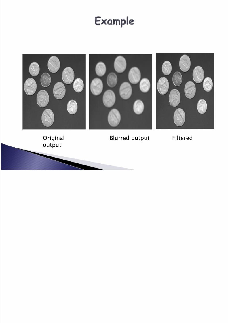
Original Blurred output Filteredoutput

8/13/2019 Unit 2 ppt2


Recap

◦ Noise models

◦ Spatial Averaging

◦ Directional Smoothing

8/13/2019 Unit 2 ppt2


Documents

Unit 2 ppt2