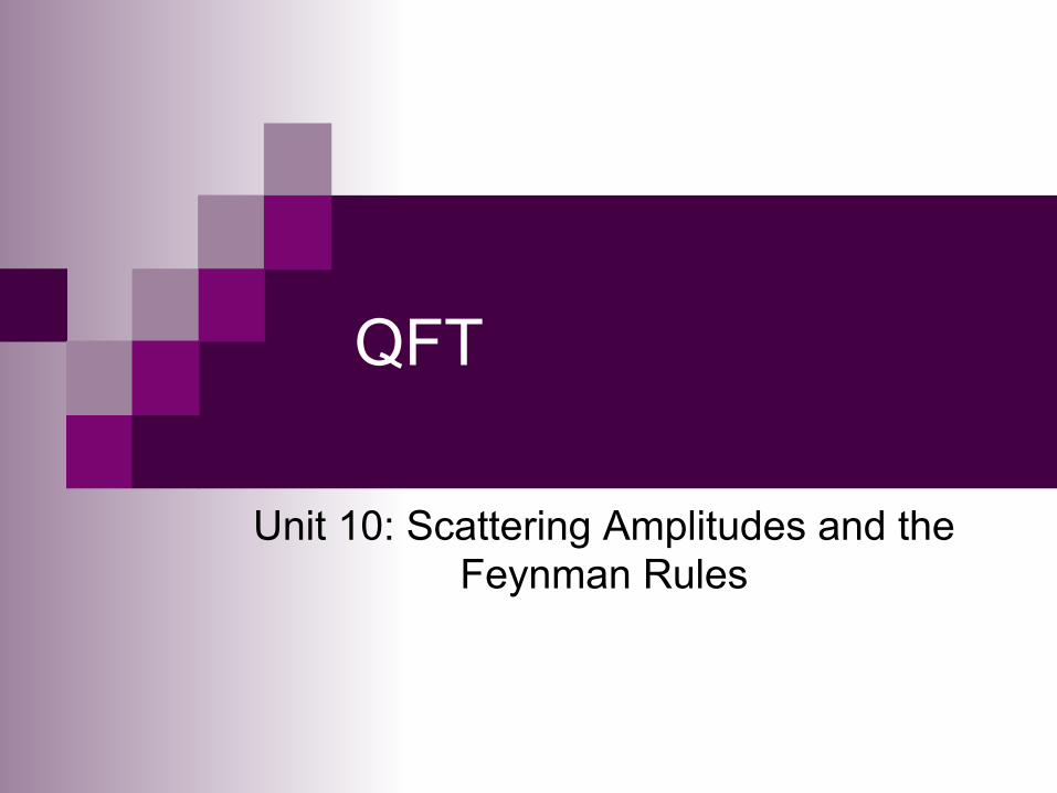
QFT

Unit 10: Scattering Amplitudes and the Feynman Rules

Overview n  Time to find a use for Z(J) that we so painstakingly

calculated in the previous section!

n  The main use is to evaluate the correlation functions in the LSZ formula, giving scattering amplitudes.

n  It turns out we can save a lot of math by introducing the Feynman Rules.

n  The next step will be to turn this scattering amplitude into a cross-section (that’s the next section).

Correlation Functions

n  Let’s start here:

¨ The first equality is taken as the definition of the propagator

¨ The second equality is our usual trick for evaluating correlation functions from path integrals, see eqns. 7.15 and 8.14.

n  For notational simplicity, we’ll write this as:

Correlation Functions, Cntd.

n Simply by doing the calculus, the right hand side becomes:

n This second term has two factors of , both of which are 0 by our choice of renormalization. Thus, only the first term survives.

Correlation Functions, Cntd. n  So, we’ve shown that:

n  What the hell is this? W(J)|J=0 is the sum of diagrams with 2 sources, with both the sources removed. ¨  The propagator endpoints are labeled x1 and x2. This will reduce

the symmetry factor. ¨  How many diagrams are there? An infinite number, but only one

has less than two vertices, it looks like this (after source removal):

¨  So, we’ve shown this fascinating fact:

x1 x2

Correlation Functions, Cntd. n  Let’s keep going with this. By doing the

calculus as before, and dropping all the terms with any factors of , we find:

n  When we insert these last three terms into the LSZ formula, the answer includes the following:

n  So, these terms represent only scattering in the trivial (non-interacting sense). Let’s drop them.

Correlation Functions, Cntd.

n  In fact, we must drop all terms except those with fully connected diagrams. These “connected correlation functions” are defined via:

n  For the two-body scattering as before, there are three connected, zeroth-order (“tree-level”) diagrams that contribute

1 1 1

2

2 2

1’ 1’

1’ 2’

2’

2’

Tree-Level Diagrams

n  Called tree-level diagrams because there are no loops. ¨  For all processes, the tree-level diagrams represent the lowest order (in

g) contributions to that process. n  Notice that we’ve stripped off (by the derivatives) the sources,

adding labels to indicate which derivative was used. n  There are 8 copies of each diagram (4! matches between δ and

source, divided by three diagrams), which cancels the symmetry factor. So, overall symmetry factor is one. ¨  In fact, all tree diagrams with the sources stripped off and the endpoints

labeled have an overall symmetry factor of one. n  This last diagram is often drawn with

the right propagators crossed, but this is not a third vertex:

1 1 1

2 2 2

1’ 1’

1’ 2’ 2’

2’

1

2

1’

2’

Correlation Functions, Cntd.

n So, we’ve shown that:

n Using the tree-level diagrams, we can calculate that:

The LSZ Formula, again

n Now let’s take this result and put it into the LSZ formula. Lots of math later, we end up with:

¨ Note that the delta function tells us that 4-momentum is conserved, which is good.

The Feynman Rules

n  But that sucked! Do we really have to do that every time we want a scattering amplitude?

n  No, we can instead define:

where the iτ is determined by the Feynman Rules

The Feynman Rules will be different for each

theory being considered

The Feynman Rules for φ3 Theory

1.  Draw external lines for each incoming and outgoing particle.

2.  Leave one end of these lines free. The other end must be hooked up to a vertex, which joins three lines. Internal lines may be drawn to do this.

3.  Draw arrows: toward vertex for incoming, away from vertex for outgoing, in arbitrary direction for internal.

4.  Assign each line a 4-momentum.

The Feynman Rules for φ3 Theory

5.  Four momentum flows along the arrows, and must be conserved at each vertex. So, internal lines have constrained four-momentum.

6.  Assign your diagram a value: n  1 for each external line n  -i/(k2 + m2 – iε) for each internal line n  iZgg for each vertex

7.  Any unfixed internal momenta must be integrated over, with measure d4l/(2π)4

The Feynman Rules for φ3 Theory

8.  Divide the value by the symmetry factor associated with exchanges of internal propagators and vertices.

9.  Include diagrams with the counterterm vertex that connects two propagators with the same 4-momentum.

n  The value of this vertex is –i((Zφ -1)k2 + (Zm - 1)m2),

and each is O(g2) because the Z’s are. 10.  The value of iτ is the sum over all these

diagrams.

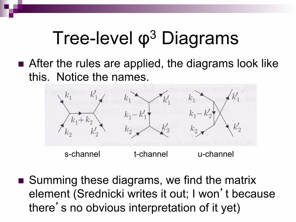
Tree-level φ3 Diagrams n  After the rules are applied, the diagrams look like

this. Notice the names.

s-channel t-channel u-channel

n  Summing these diagrams, we find the matrix element (Srednicki writes it out; I won’t because there’s no obvious interpretation of it yet)

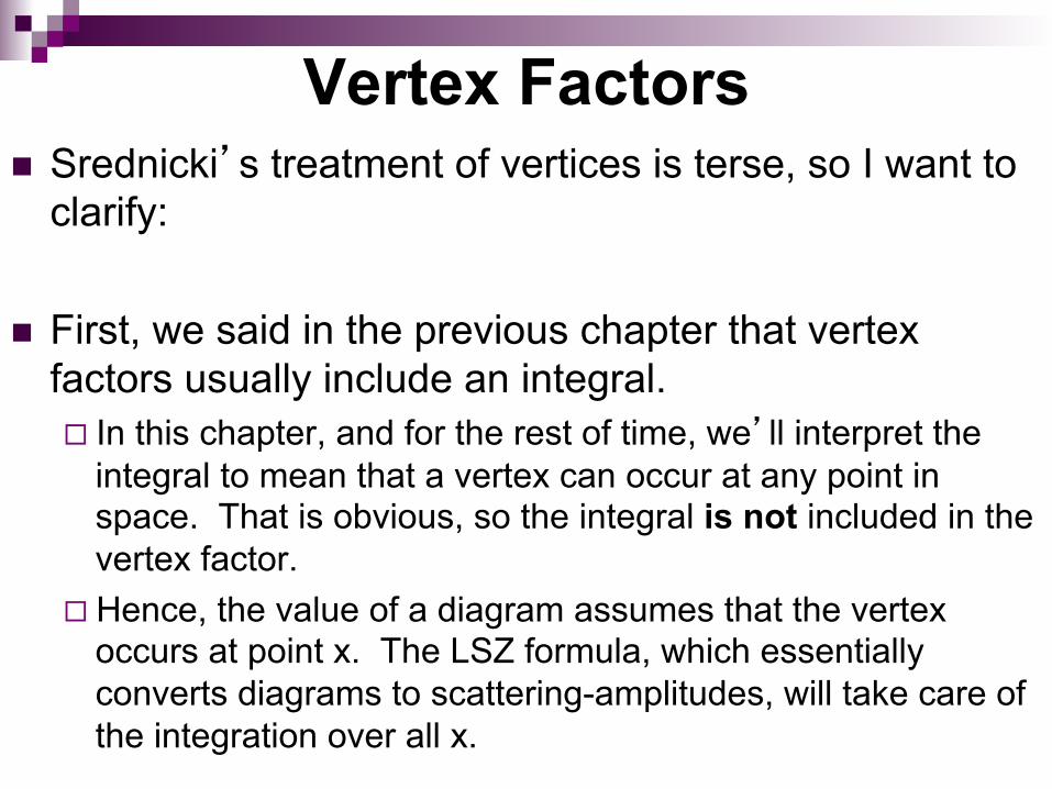
Vertex Factors n  Srednicki’s treatment of vertices is terse, so I want to

clarify:

n  First, we said in the previous chapter that vertex factors usually include an integral. ¨  In this chapter, and for the rest of time, we’ll interpret the

integral to mean that a vertex can occur at any point in space. That is obvious, so the integral is not included in the vertex factor.

¨ Hence, the value of a diagram assumes that the vertex occurs at point x. The LSZ formula, which essentially converts diagrams to scattering-amplitudes, will take care of the integration over all x.

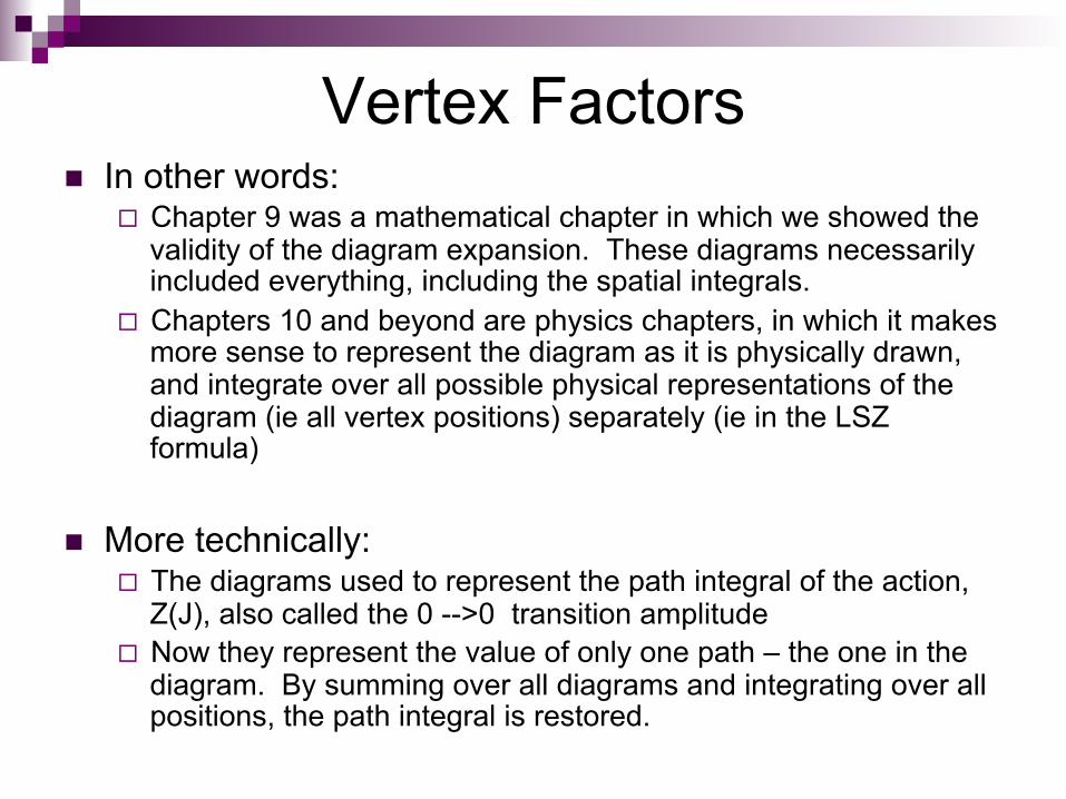
Vertex Factors n  In other words:

¨  Chapter 9 was a mathematical chapter in which we showed the validity of the diagram expansion. These diagrams necessarily included everything, including the spatial integrals.

¨  Chapters 10 and beyond are physics chapters, in which it makes more sense to represent the diagram as it is physically drawn, and integrate over all possible physical representations of the diagram (ie all vertex positions) separately (ie in the LSZ formula)

n  More technically: ¨  The diagrams used to represent the path integral of the action,

Z(J), also called the 0 -->0 transition amplitude ¨  Now they represent the value of only one path – the one in the

diagram. By summing over all diagrams and integrating over all positions, the path integral is restored.

Calculating Vertex Factors n  The procedure for determining vertex factors is a little

ambiguous, so let’s specify it here:

where i sums over all the propagators in the vertex.

n  Where does this come from? is the term in Z(J) represented by the vertices. Once the three incoming propagators are removed by the partial derivative, the remainder is the value assigned to the vertex itself (there may also be a plane wave, but that can be ignored)

n  Remember that Feynman Diagrams live in momentum space, hence the momentum derivative.

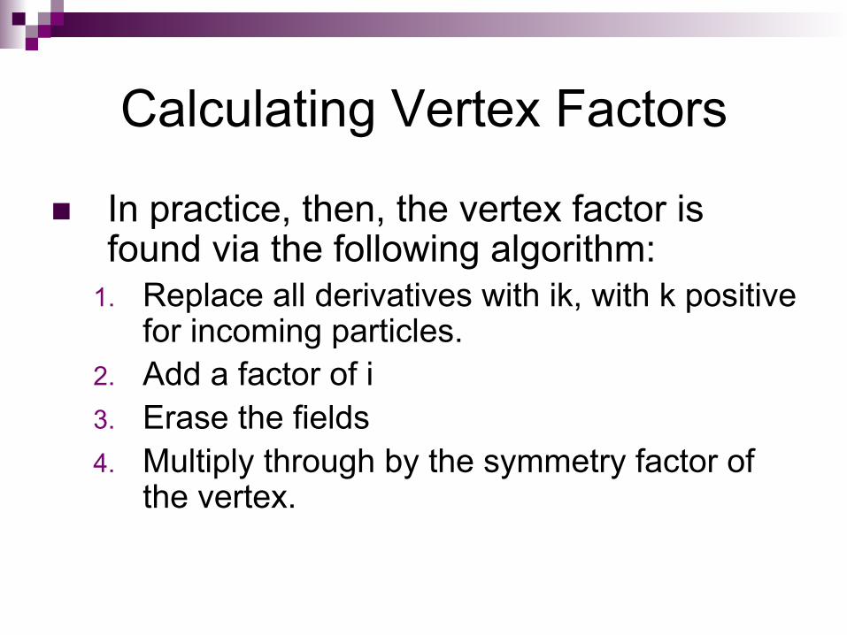
Calculating Vertex Factors

n  In practice, then, the vertex factor is found via the following algorithm:

1.  Replace all derivatives with ik, with k positive for incoming particles.

2.  Add a factor of i 3.  Erase the fields 4.  Multiply through by the symmetry factor of

the vertex.

Conclusions

n We now have the scattering amplitude. ¨ This procedure will work in general, but notice

that our specific results – including our Feynman Rules – only work for φ3 theory.

n Scattering amplitudes are not something that can be measured in a lab. Our next step is to use scattering amplitudes to determine cross-sections, which can be experimentally measured.