Embed Size (px)
Citation preview
Unit 1 – Review of Mathematical Theory
1
Dixita Kagathara, CE Department | 2160704 – Theory of Computation
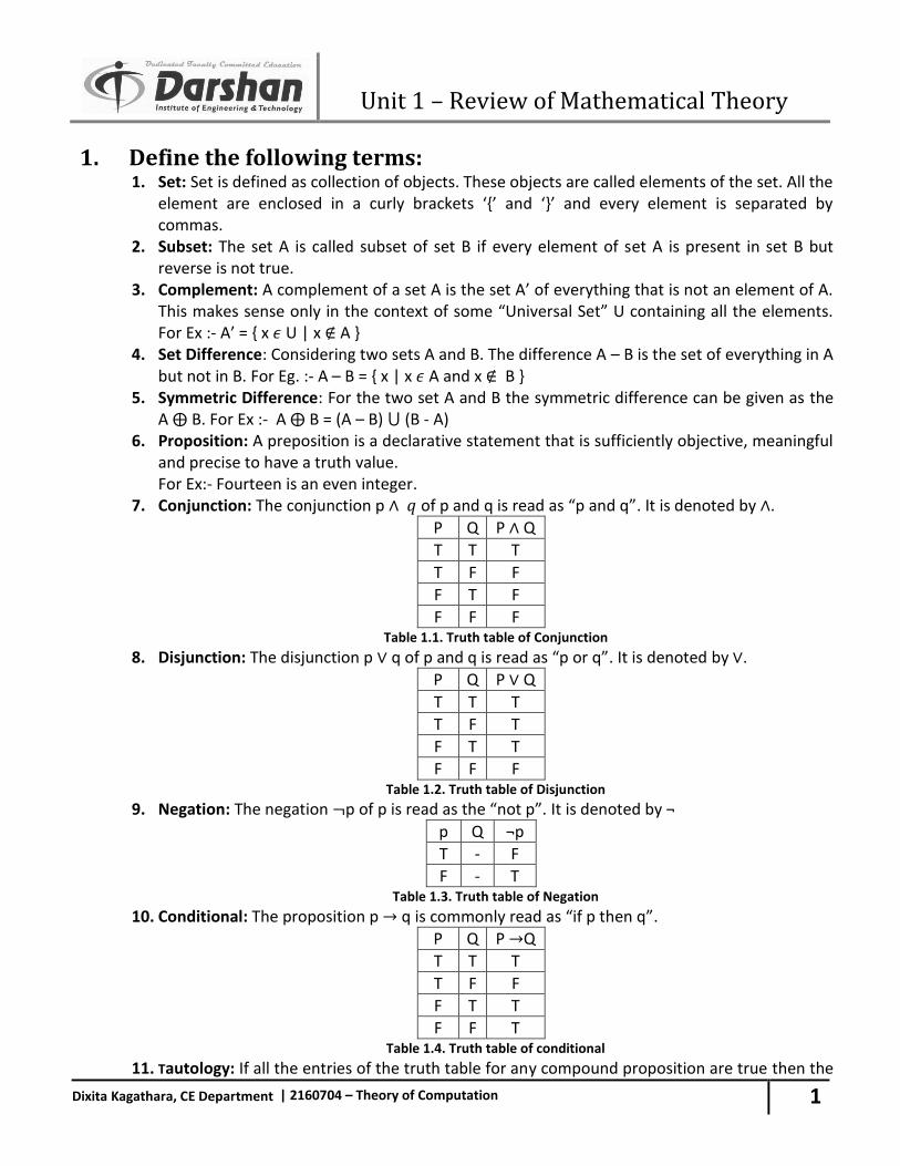
1. Define the following terms: 1. Set: Set is defined as collection of objects. These objects are called elements of the set. All the
element are enclosed in a curly brackets ‘{’ and ‘}’ and every element is separated by commas.
2. Subset: The set A is called subset of set B if every element of set A is present in set B but reverse is not true.
3. Complement: A complement of a set A is the set A’ of everything that is not an element of A. This makes sense only in the context of some “Universal Set” U containing all the elements. For Ex :- A’ = { x U | x A }
4. Set Difference: Considering two sets A and B. The difference A – B is the set of everything in A but not in B. For Eg. :- A – B = { x | x A and x B }
5. Symmetric Difference: For the two set A and B the symmetric difference can be given as the A B. For Ex :- A B = (A – B) (B - A)
6. Proposition: A preposition is a declarative statement that is sufficiently objective, meaningful and precise to have a truth value. For Ex:- Fourteen is an even integer.
7. Conjunction: The conjunction p of p and q is read as “p and q”. It is denoted by .
P Q P Q
T T T
T F F
F T F
F F F Table 1.1. Truth table of Conjunction
8. Disjunction: The disjunction p q of p and q is read as “p or q”. It is denoted by .
P Q P Q
T T T
T F T
F T T
F F F Table 1.2. Truth table of Disjunction
9. Negation: The negation p of p is read as the “not p”. It is denoted by ¬
p Q ¬p
T - F
F - T Table 1.3. Truth table of Negation
10. Conditional: The proposition p q is commonly read as “if p then q”.
P Q P Q
T T T
T F F
F T T
F F T Table 1.4. Truth table of conditional
11. Tautology: If all the entries of the truth table for any compound proposition are true then the
Unit 1 – Review of Mathematical Theory
2
Dixita Kagathara, CE Department | 2160704 – Theory of Computation
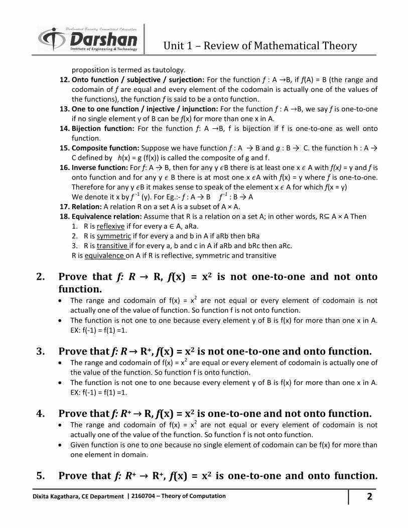
proposition is termed as tautology. 12. Onto function / subjective / surjection: For the function f : A B, if f(A) = B (the range and
codomain of f are equal and every element of the codomain is actually one of the values of the functions), the function f is said to be a onto function.
13. One to one function / injective / injunction: For the function f : A B, we say f is one-to-one if no single element y of B can be f(x) for more than one x in A.
14. Bijection function: For the function f: A B, f is bijection if f is one-to-one as well onto function.
15. Composite function: Suppose we have function f : A → B and g : B → C. the function h : A → C defined by h(x) = g (f(x)) is called the composite of g and f.
16. Inverse function: For f: A → B, then for any y B there is at least one x A with f(x) = y and f is onto function and for any y B there is at most one x A with f(x) = y where f is one-to-one. Therefore for any y B it makes sense to speak of the element x A for which f(x = y) We denote it x by f -1 (y). For Eg.:- f : A → B f -1 : B → A
17. Relation: A relation R on a set A is a subset of A × A. 18. Equivalence relation: Assume that R is a relation on a set A; in other words, R⊆ A × A Then
1. R is reflexive if for every a ∈ A, aRa. 2. R is symmetric if for every a and b in A if aRb then bRa 3. R is transitive if for every a, b and c in A if aRb and bRc then aRc. R is equivalence on A if R is reflective, symmetric and transitive
2. Prove that f: R → R, f(x) = x2 is not one-to-one and not onto function.
The range and codomain of f(x) = x2 are not equal or every element of codomain is not actually one of the value of function. So function f is not onto function.
The function is not one to one because every element y of B is f(x) for more than one x in A. EX: f(-1) = f(1) =1.
3. Prove that f: R → R+, f(x) = x2 is not one-to-one and onto function. The range and codomain of f(x) = x2 are equal or every element of codomain is actually one of
the value of the function. So function f is onto function.
The function is not one to one because every element y of B is f(x) for more than one x in A. EX: f(-1) = f(1) =1.
4. Prove that f: R+ → R, f(x) = x2 is one-to-one and not onto function. The range and codomain of f(x) = x2 are not equal or every element of codomain is not
actually one of the value of the function. So function f is not onto function.
Given function is one to one because no single element of codomain can be f(x) for more than one element in domain.
5. Prove that f: R+ → R+, f(x) = x2 is one-to-one and onto function.
Unit 1 – Review of Mathematical Theory
3
Dixita Kagathara, CE Department | 2160704 – Theory of Computation
(bijection). The range and codomain of f(x) = x2 are equal or every element of codomain is actually one of
the value of the function. So function f is onto function.
Given function is one to one because no single element of codomain can be f(x) for more than one element in domain.
The function f(x) = x2 is onto function as well as one-to-one function. So, it is called as bijection function.
6. Give quantified statement saying that p is prime. Let us consider that statement “P is prime” involving the free variable p over the universe N of
natural number.
We take our definition of a prime number, a number greater than 1 whose only divisor are itself and 1.
The first statement is now to express the fact that one number is a divisor of another.
The statement “k is a divisor of p” means that p is a multiple of k or there is an integer m with p = m * k
Next saying that the only divisors of p are p and 1 is the same as saying that every divisor of p is either p or 1.
Adapting the statement that “for every k, if k is a divisor of p, then k is either p or 1”.
Considering all these together we get that “p is prime”.{ ( p > 1 ) ∀ k (∃m ( p = m * k ) )→ (k = 1) (k = p ) }
7. What is Proof? A proof of a statement is essentially just a convincing argument that the statement is true.
There are several methods for establishing a proof, some of them are : 1. Direct Proof 2. By Contradiction 3. By Contra positive 4. By Mathematical Induction
8. For any integers a and b, if a and b are odd, then ab is odd. Proof:
An integer n is odd if there exists an integer x so that n=2x+1.
Now let a and b be any odd integers. Then according to this definition, there is an integer x so that a=2x+1, and there is an integer y so that b=2y+1.
We wish to show that there is an integer z so that ab=2z+1. Let us therefore calculate ab: =(2x+1)(2y+1) =4xy+2x+2y+1 =2(2xy+x+y)+1
Since we have shown that is a z, namely, 2xy+x+y, so that ab=2z+1, the proof is complete.
Example:
Unit 1 – Review of Mathematical Theory
4
Dixita Kagathara, CE Department | 2160704 – Theory of Computation
X=45 & y= 11 xy= 2(2xy+x+y)+1 = 2(2(45)(11)+45+11)+1 = 2(1046)+1 xy=2093 Hence proved.
9. To Prove: For every three positive integers i, j, and n, if i*j = n,
then i ≤ or j ≤ . The statement we wish to prove is of the general form “for every x, if p(x) then q(x).” For each
x, the statement “if p(x) then q(x)” is logically equivalent to “if not p(x) then not q(x).” and therefore the statement we want to prove is equivalent to this: For any positive integer i, j,
and n, if it is not the case that i ≤ or j ≤ then i*j≠n.
If it is not true that i ≤ or j ≤ , then i > and j> . A generally accepted fact from mathematical is that if a and b are number with a> b, and c is a number >0, then ac>bc.
Applying this to the inequality i> with c=j, we obtain i*j > * j. since n>0, we know that
>0, and we may apply the same fact again to the inequality j> , this time letting c= , to
obtain j > =n. We now have i*j > j >n, and it follow that i*j ≠ n.
Hence, the proof is complete.
10. (Root two) is irrational number. (Most IMP) Suppose for the sake of contradiction that is rational. Then there are integers m’ and n’
with = m’/ n’.
By dividing both m’ and n’ by all the factors that are common to both, we obtain =m/n, for
some integer m and n having no common factors. Since m/n= , m= n . Squaring both sides of this equation, we obtain m2=2n2, and therefore m2 is even.
If a and b are odd, then ab is odd. Since a conditional statement is logically equivalent to its contra positive, we may conclude that for any a and b, if ab is not odd, then either a is not odd or b is not odd.
However, an integer is not odd if and only if it is even, and so for any a and b, if ab is even, m must be even.
This means that for some k, m=2k. Therefore, (2k) 2=2n2.
Simplifying this and canceling 2 from both side, we obtain 2k2=n2. Therefore n2 is even.
The same argument that we have already used to show that n must be even, and so n=2j for some j.
We have shown that m and n are both divisible by 2. This contradicts the previous statement
that m and n have no common factor. The assumption that is rational therefore it leads to
a contradiction, and the conclusion is that is irrational.
11. Explain principle of Mathematical Induction.
Unit 1 – Review of Mathematical Theory
5
Dixita Kagathara, CE Department | 2160704 – Theory of Computation
Suppose P(n) is a statement involving an integer n. Then to prove that P(n) is true for every n>=n0, it is sufficient to show these two things:
1. P (n0) is true. 2. For every k>= n0, if P(k) is true, P(k+1) is true.
12. Prove
Step-1: Basic step We must show that p(0) is true. 0 = 0(0+1)/2 And, this is obviously true. Step-2: Induction Hypothesis k >= 0 and
1+2+3+4…..+k =
Step-3: Proof of Induction p(k+1) = 1+2+3+….+k+(k+1)
=
+ (k+1) by induction hypothesis
=
=
P(k+1) =
Hence by principle of mathematical induction is true.
13. Prove
Step-1: Basic We must show that p(0) is true.
P(0)=
=0
And, this is obviously true. Step-2: Induction Hypothesis k >= 0 and
P(k) = 1+4+9+….k2 =
Step-3:Proof of Induction
P(k+1) =
+ (k+1)2
=
=
=
Unit 1 – Review of Mathematical Theory
6
Dixita Kagathara, CE Department | 2160704 – Theory of Computation
=
=
=
=
=
=
=
Hence by principle of mathematical induction is true.
14. Prove
Step-1: Basic We must show that p(0) is true.
P(0) =
=0
And, this is obviously true. Step-2: Induction Hypothesis k >= 0 and
p(k)=
Step-3: Proof of Induction
p(k+1) =
=
=
=
=
=
=
Unit 1 – Review of Mathematical Theory
7
Dixita Kagathara, CE Department | 2160704 – Theory of Computation
=
=
=
=
Hence by principle of mathematical induction
is true.
15. Prove 7+ 13+19+…..+(6n+1)= n(3n+4) Step-1: Basic
We must show that p(0) is true. P(0)= 0(3(0)+4)=0 And, this is obviously true. Step-2: Induction Hypothesis k >= 0 and p(k) = 7+13+19+…..+(6k+1)=k(3k+4) Step-3: Proof of Induction P(k+1) = 7+13+19+…..+(6k+1)+(6(k+1)+1) = k(3k+4)+(6(k+1)+1) = k(3k+4)+(6k+6+1) = 3k2+4k+6k+7 = 3k2+10k+7 = 3k2+3k+7k+7 = 3k(k+1)+7(k+1) = (k+1)(3k+7) = (k+1)(3k+3+4) = (k+1)(3(k+1)+4) Hence by principle of mathematical induction is true.
16. Prove 1+
Step-1: Basic We must show that p(0) is true. P(0)= (0+1)! =(1)! = 1 And, this is obviously true. Step-2: Induction Hypothesis k >= 0 and p(k) = 1+(1+4+18+…..+(k*k!)) = (k+1)! Step-3: Proof of Induction
Unit 1 – Review of Mathematical Theory
8
Dixita Kagathara, CE Department | 2160704 – Theory of Computation
P(k+1) = 1+(1+4+18+…..+(k*k!) + (k+1)*(k+1)!) = (k+1)! + (k+1)(k+1)!) = (k+1)! (1+(k+1)) = (k+1)! ((k+1)+1) = ((k+1) + 1)! Hence by principle of mathematical induction
is true.
17. Prove
Step-1: Basic We must show that P(1) is true. P(1) = (1)2 = 1 And, this is obviously true. Step-2: Induction Hypothesis k >= 0 and p(k) = 1+3+5+…..+(2k-1)=k2 Step-3: Proof of Induction P(k+1) = 1+3+5+….+(2k-1)+(2(k+1)-1)
= k2 + (2(k+1)-1) = k2 + (2k+2-1) = k2 + 2k+1 =(k+1)2
Hence by principle of mathematical induction is
true.
18. Prove that 2n>n3 where n>=10, Using Principle of Mathematical Induction.
Step-1: Basic step We must show that p(10) is true. 210=1024 and 103=1000 So,1024>1000 And, this is obviously true. Step-2: Induction Hypothesis For k>=10 P(k)= 2k>k3 Statement to be shown in Induction step is, P(k+1)=2k+1>(k+1)3 Step-3: Proof of Induction 2k+1>(k+1)3
Where, 2k+1=(2k )(2)>2k (1.331)
>2k (1+
)3
Unit 1 – Review of Mathematical Theory
9
Dixita Kagathara, CE Department | 2160704 – Theory of Computation
>2k(1+
)3 for k>=10
>(
)3 (2k)
>(
)3 (k3) ,because 2k>k3
(2k )(2)>(k+1)3
2k+1>(k+1)3 ;k>=10 Hence by principle of mathematical induction 2n>n3 is true.
19. Prove n(n2+5) is divisible by 6 for n>=0, Using Principle of Mathematical Induction.
Step-1: Basic step We must show that p(0) is true. P(0)=0(02+5)=0*6/6=0 And, this is obviously true. Step-2: Induction Hypothesis For k>=0 and P(k)=k(k2+5) is divisible by 6. Statement to be shown in Induction step is, P(k+1)=(k+1)[(k+1)2+5] is divisible by 6. Step-3: Proof of Induction (k+1)[(k+1)2+5] =k[(k+1)2+5]+1[(k+1)2+5] =k(k2+2k+1+5)+(k2+2k+1+5) =k3+2k2+k+5k+(k2+2k+6) =k(k2+5)+k(2k+1)+(k2+2k+6) = k(k2+5)+2k2+k+k2+2k+6 = k(k2+5)+3k2+3k+6 = k(k2+5)+3k(k+1)+6
Here, k(k2+5) is divisible by 6 ,given in induction hypothesis.
In Second term k and k+1 are consecutive. So, one number is even and one is odd. So, even number is always multiple of 2 and here 3 is also present .So, second term having (2*3) is also divisible by 6.
Last term 6 is obviously divisible by 6.Hence proved.
20. Strong Principle of Mathematical Induction Suppose p(n) is a statement involving on integer n then to prove that p(n) is true for every n>= n0.
It is sufficient to show these two condition 1) P(n0) is true 2) For any k >=n0 , if p(n) is true for every n satisfying n0<=n<=k then p(k+1) is true.
Unit 1 – Review of Mathematical Theory
10
Dixita Kagathara, CE Department | 2160704 – Theory of Computation
21. Prove that Integer Bigger than 2 have prime factorization using strong PMI
Basic step:
P(2) is the statement that 2 is either a prime or a product of two or more primes. This is true because 2 is prime.
Induction hypothesis:
K ≥ 2, and for every n with 2≤n≤k,n is either prime or a product of two or more primes. Statement to be shown in induction step:
K+1 is either prime or a product of two or more primes. Proof of induction step:
We consider two cases. If k+1 is prime, the statement p(k+1) is true. Otherwise, by definition of a prime, k+1 = r*s, for some positive integer r and s, neither of which is 1 or k+1. It follows that 2 ≤ r ≤ k and 2 ≤ s ≤ k. therefore, by the induction hypothesis; both r and s are either prime or the product of two or more primes.
Therefore, their product k+1 is the product of two or more primes, and p(k+1) is true.
Hence, integer bigger than 2 have prime factorization.
Unit 2 – Regular Languages & Finite Automata
1
Dixita Kagathara, CE Department | 2160704 – Theory of Computation
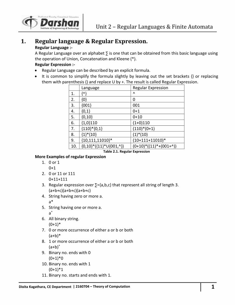
1. Regular language & Regular Expression. Regular Language :-
A Regular Language over an alphabet ∑ is one that can be obtained from this basic language using the operation of Union, Concatenation and Kleene (*). Regular Expression :-
Regular Language can be described by an explicit formula.
It is common to simplify the formula slightly by leaving out the set brackets {} or replacing them with parenthesis () and replace U by +. The result is called Regular Expression.
Language Regular Expression
1. {^} ^
2. {0} 0
3. {001} 001
4. {0,1} 0+1
5. {0,10} 0+10
6. {1,0}110 (1+0)110
7. {110}*{0,1} (110)*(0+1)
8. {1}*{10} (1)*(10)
9. {10,111,11010}* (10+111+11010)*
10. {0,10}*({11}*U{001,^}) (0+10)*((11)*+(001+^)) Table 2.1. Regular Expression
More Examples of regular Expression 1. 0 or 1
0+1 2. 0 or 11 or 111 0+11+111 3. Regular expression over ∑={a,b,c} that represent all string of length 3.
(a+b+c)(a+b+c)(a+b+c) 4. String having zero or more a. a* 5. String having one or more a. a+ 6. All binary string. (0+1)* 7. 0 or more occurrence of either a or b or both (a+b)* 8. 1 or more occurrence of either a or b or both (a+b)+ 9. Binary no. ends with 0 (0+1)*0 10. Binary no. ends with 1 (0+1)*1 11. Binary no. starts and ends with 1.
Unit 2 – Regular Languages & Finite Automata
2
Dixita Kagathara, CE Department | 2160704 – Theory of Computation
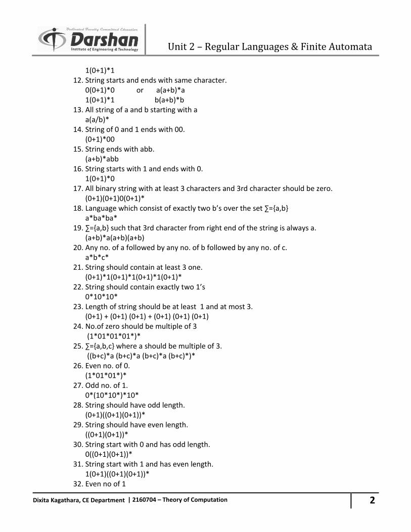
1(0+1)*1 12. String starts and ends with same character. 0(0+1)*0 or a(a+b)*a 1(0+1)*1 b(a+b)*b 13. All string of a and b starting with a a(a/b)* 14. String of 0 and 1 ends with 00. (0+1)*00 15. String ends with abb. (a+b)*abb 16. String starts with 1 and ends with 0. 1(0+1)*0 17. All binary string with at least 3 characters and 3rd character should be zero. (0+1)(0+1)0(0+1)* 18. Language which consist of exactly two b’s over the set ∑={a,b} a*ba*ba* 19. ∑={a,b} such that 3rd character from right end of the string is always a. (a+b)*a(a+b)(a+b) 20. Any no. of a followed by any no. of b followed by any no. of c. a*b*c* 21. String should contain at least 3 one. (0+1)*1(0+1)*1(0+1)*1(0+1)* 22. String should contain exactly two 1’s 0*10*10* 23. Length of string should be at least 1 and at most 3. (0+1) + (0+1) (0+1) + (0+1) (0+1) (0+1) 24. No.of zero should be multiple of 3 (1*01*01*01*)* 25. ∑={a,b,c} where a should be multiple of 3. ((b+c)*a (b+c)*a (b+c)*a (b+c)*)* 26. Even no. of 0. (1*01*01*)* 27. Odd no. of 1. 0*(10*10*)*10* 28. String should have odd length. (0+1)((0+1)(0+1))* 29. String should have even length. ((0+1)(0+1))* 30. String start with 0 and has odd length. 0((0+1)(0+1))* 31. String start with 1 and has even length. 1(0+1)((0+1)(0+1))* 32. Even no of 1
Unit 2 – Regular Languages & Finite Automata
3
Dixita Kagathara, CE Department | 2160704 – Theory of Computation
(0*10*10*)* 33. String of length 6 or less (0+1+^)6 34. String ending with 1 and not contain 00. (1+01)+ 35. All string begins or ends with 00 or 11. (00+11)(0+1)*+(0+1)*(00+11) 36. Language of all string containing both 11 and 00 as substring. ((0+1)*00(0+1)*11(0+1)*)+ ((0+1)*11(0+1)*00(0+1)*) 37. Language of C identifier.
(_+L)(_+L+D)*
2. Definition of Finite Automata. A finite Automata or finite state machine is a 5-tuple(Q,∑,q0,A,δ) where,
Q is finite set of states; ∑ is finite alphabet of input symbols; q0 ∈ Q (Initial state); A (set of accepting states); δ is a function from Q×∑Q(Transition function);
For any element q of Q and any symbol a ∈ ∑, we interpret δ (q, a) as the state to which the Finite Automata moves, if it is in state q and receives the input a. Application of finite automata A finite automaton is used to solve several common types of computer algorithm. Some of them are:
1. Design of digital circuit. 2. String matching. 3. Communication protocols for information exchange. 4. Lexical analysis phase of a compiler.
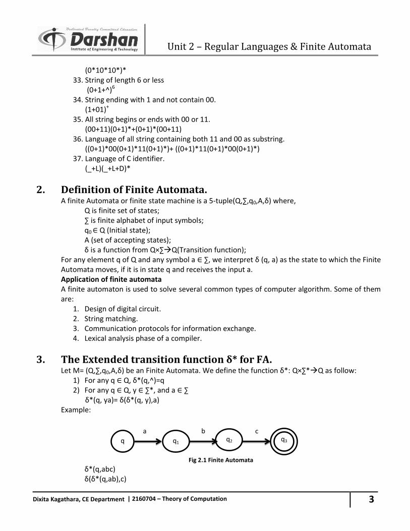
3. The Extended transition function δ* for FA. Let M= (Q,∑,q0,A,δ) be an Finite Automata. We define the function δ*: Q×∑*Q as follow:
1) For any q ∈ Q, δ*(q,^)=q 2) For any q ∈ Q, y ∈ ∑*, and a ∈ ∑
δ*(q, ya)= δ(δ*(q, y),a) Example:
Fig 2.1 Finite Automata
δ*(q,abc) δ(δ*(q,ab),c)
q q1 q2
a b
c q3
Unit 2 – Regular Languages & Finite Automata
4
Dixita Kagathara, CE Department | 2160704 – Theory of Computation
δ(δ*( δ*(q,a),b),c) δ(δ(δ* (q,^a),b),c) δ(δ(δ(δ*(q,^),a),b),c) δ(δ(δ(q,a),b),c) δ(δ(q1,b),c) δ(q2,c) q3
4. Acceptance by an Finite Automata. Let M= (Q1, ∑, q0, A, δ) be an FA. A string x ∈ ∑* is accepted by M if δ*(q0, x) ∈ A. If string is not
accepted, we can say it is rejected by M. The language accepted by M, or the language recognized by M, is the set L(M) = {x ∈ ∑*/x is accepted by M} If L is any Language over ∑, L is accepted or recognized by M if and only if L=L(M).
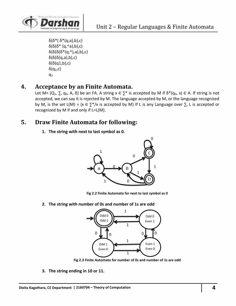
5. Draw Finite Automata for following:
1. The string with next to last symbol as 0.
Fig 2.2 Finite Automata for next to last symbol as 0
2. The string with number of 0s and number of 1s are odd
Fig 2.3 Finite Automata for number of 0s and number of 1s are odd
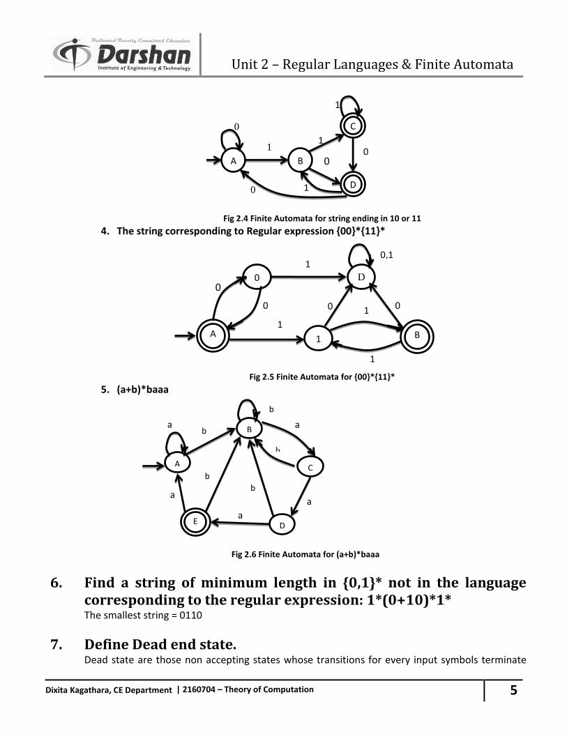
3. The string ending in 10 or 11.
1 Odd 0
Odd 1
1
1
0 0
1
0 0
Odd 0
Even 1
Even 1
Even 0
Odd 1
Even 0
0 B
C
D 1 0
1
1
0
1 A
0
Unit 2 – Regular Languages & Finite Automata
5
Dixita Kagathara, CE Department | 2160704 – Theory of Computation
A
0 D
1
0
0
1
1
0
0,1
0
0
1
1
1
B
Fig 2.4 Finite Automata for string ending in 10 or 11
4. The string corresponding to Regular expression {00}*{11}*
Fig 2.5 Finite Automata for {00}*{11}*
5. (a+b)*baaa
Fig 2.6 Finite Automata for (a+b)*baaa
6. Find a string of minimum length in {0,1}* not in the language corresponding to the regular expression: 1*(0+10)*1*
The smallest string = 0110
7. Define Dead end state. Dead state are those non accepting states whose transitions for every input symbols terminate
a
E
b
A
B b
C
a
D a
b b
a
a
b
1
A
1
B
C
D 0 1
0
0
1
0
Unit 2 – Regular Languages & Finite Automata
6
Dixita Kagathara, CE Department | 2160704 – Theory of Computation
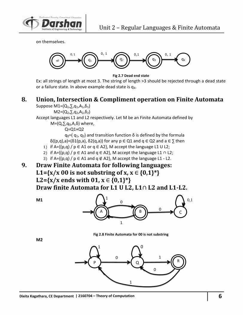
on themselves.
Fig 2.7 Dead end state
Ex: all strings of length at most 3. The string of length >3 should be rejected through a dead state or a failure state. In above example dead state is q4.
8. Union, Intersection & Compliment operation on Finite Automata Suppose M1=(Q1,∑,q1,A1,δ1)
M2=(Q2,∑,q2,A2,δ2) Accept languages L1 and L2 respectively. Let M be an Finite Automata defined by M=(Q,∑,q0,A,δ) where, Q=Q1×Q2 q0=( q1, q2) and transition function δ is defined by the formula δ((p,q),a)=(δ1(p,a), δ2(q,a)) for any p ∈ Q1 and q ∈ Q2 and a ∈ ∑ then
1) if A={(p,q) / p ∈ A1 or q ∈ A2}, M accept the language L1 U L2; 2) if A={(p,q) / p ∈ A1 and q ∈ A2}, M accept the language L1 ∩ L2; 3) if A={(p,q) / p ∈ A1 and q A2}, M accept the language L1 - L2.
9. Draw Finite Automata for following languages: L1={x/x 00 is not substring of x, x ∈ {0,1}*} L2={x/x ends with 01, x ∈ {0,1}*} Draw finite Automata for L1 U L2, L1∩ L2 and L1-L2.
M1
Fig 2.8 Finite Automata for 00 is not substring M2
q1 q2
0, 1 0, 1 0,1
q3 q0 q4 0, 1
A B
1
C
0,1
0
0
1
P
1
Q R
0
0 1
0
1
Unit 2 – Regular Languages & Finite Automata
7
Dixita Kagathara, CE Department | 2160704 – Theory of Computation
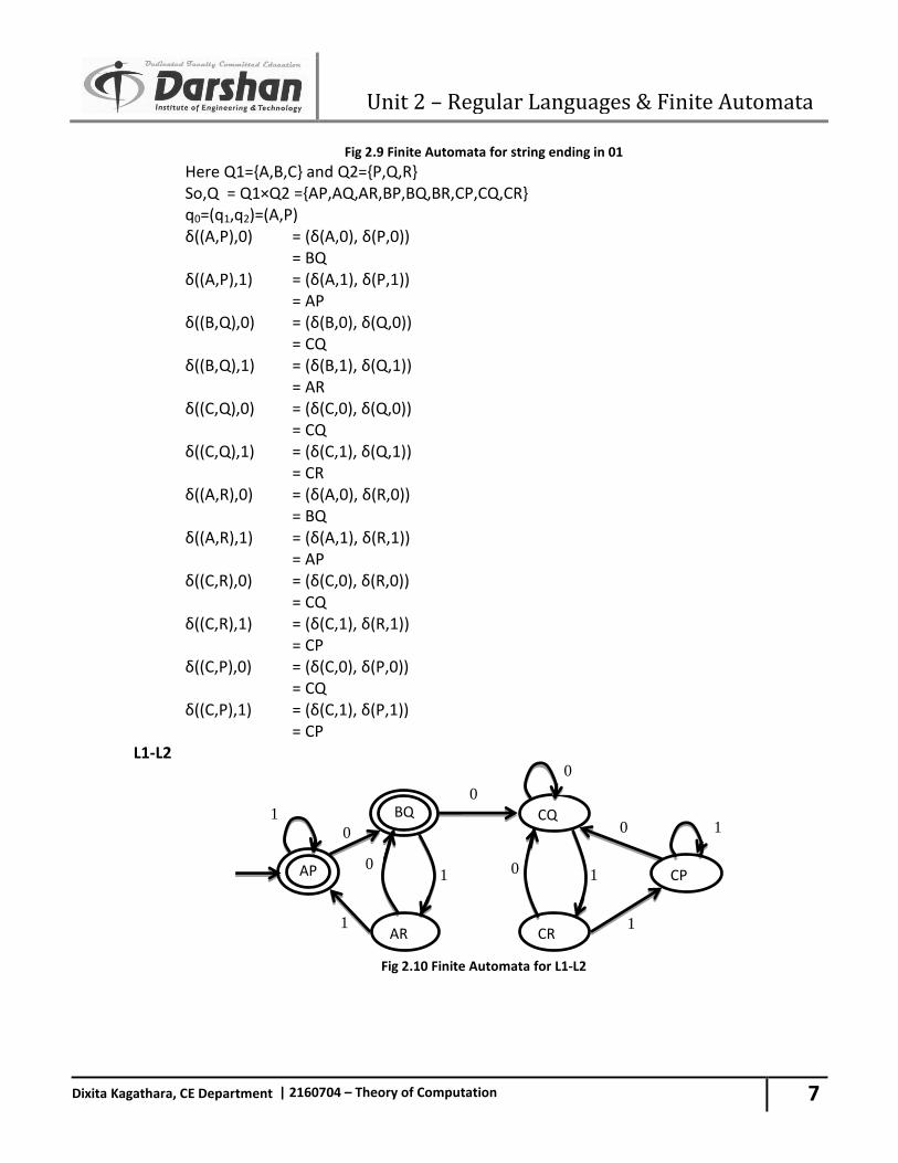
Fig 2.9 Finite Automata for string ending in 01 Here Q1={A,B,C} and Q2={P,Q,R} So,Q = Q1×Q2 ={AP,AQ,AR,BP,BQ,BR,CP,CQ,CR} q0=(q1,q2)=(A,P) δ((A,P),0) = (δ(A,0), δ(P,0)) = BQ δ((A,P),1) = (δ(A,1), δ(P,1)) = AP δ((B,Q),0) = (δ(B,0), δ(Q,0)) = CQ δ((B,Q),1) = (δ(B,1), δ(Q,1)) = AR δ((C,Q),0) = (δ(C,0), δ(Q,0)) = CQ δ((C,Q),1) = (δ(C,1), δ(Q,1)) = CR δ((A,R),0) = (δ(A,0), δ(R,0)) = BQ δ((A,R),1) = (δ(A,1), δ(R,1)) = AP δ((C,R),0) = (δ(C,0), δ(R,0)) = CQ δ((C,R),1) = (δ(C,1), δ(R,1)) = CP δ((C,P),0) = (δ(C,0), δ(P,0)) = CQ δ((C,P),1) = (δ(C,1), δ(P,1)) = CP L1-L2
Fig 2.10 Finite Automata for L1-L2
AP
BQ
AR
CQ
CR
0
0
CP
1
0
1
0
0
1
0 1 1
0
1
Unit 2 – Regular Languages & Finite Automata
8
Dixita Kagathara, CE Department | 2160704 – Theory of Computation
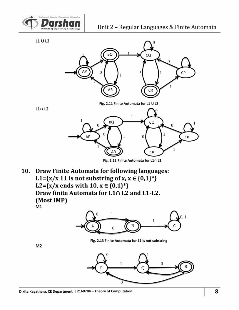
L1 U L2
Fig. 2.11 Finite Automata for L1 U L2 L1∩ L2
10. Draw Finite Automata for following languages: L1={x/x 11 is not substring of x, x ∈ {0,1}*} L2={x/x ends with 10, x ∈ {0,1}*} Draw finite Automata for L1∩ L2 and L1-L2. (Most IMP)
M1
Fig. 2.13 Finite Automata for 11 is not substring M2
AP
BQ CQ
CP
1
1
1
0
0
1
0 1
1
0
1
AR CR
CQ 0
CP
1
1
1
0
0
1
0 1 1
0
1
AR
BQ
AP
CR
0, 1 1
1
A
0
B C 0
0
P 0
Q R 1
0 1
1
Fig. 2.12 Finite Automata for L1∩ L2
Unit 2 – Regular Languages & Finite Automata
9
Dixita Kagathara, CE Department | 2160704 – Theory of Computation
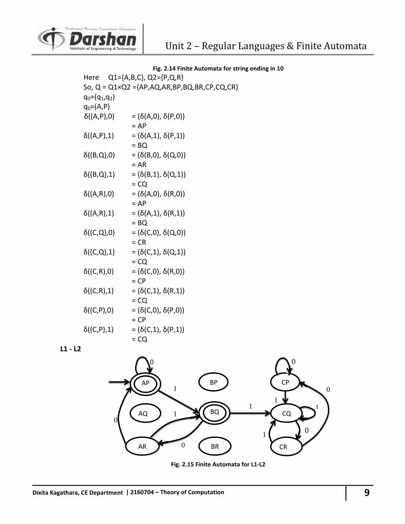
Fig. 2.14 Finite Automata for string ending in 10 Here Q1={A,B,C}, Q2={P,Q,R} So, Q = Q1×Q2 ={AP,AQ,AR,BP,BQ,BR,CP,CQ,CR} q0=(q1,q2) q0=(A,P) δ((A,P),0) = (δ(A,0), δ(P,0)) = AP δ((A,P),1) = (δ(A,1), δ(P,1)) = BQ δ((B,Q),0) = (δ(B,0), δ(Q,0)) = AR δ((B,Q),1) = (δ(B,1), δ(Q,1)) = CQ δ((A,R),0) = (δ(A,0), δ(R,0)) = AP δ((A,R),1) = (δ(A,1), δ(R,1)) = BQ δ((C,Q),0) = (δ(C,0), δ(Q,0)) = CR δ((C,Q),1) = (δ(C,1), δ(Q,1)) = CQ δ((C,R),0) = (δ(C,0), δ(R,0)) = CP δ((C,R),1) = (δ(C,1), δ(R,1)) = CQ δ((C,P),0) = (δ(C,0), δ(P,0)) = CP δ((C,P),1) = (δ(C,1), δ(P,1)) = CQ L1 - L2
Fig. 2.15 Finite Automata for L1-L2
1
0 AQ
AR
BP
BR
CP
CQ 1
1
0
1
0
1 0
1
0
0
BQ
CR
AP
Unit 2 – Regular Languages & Finite Automata
10
Dixita Kagathara, CE Department | 2160704 – Theory of Computation
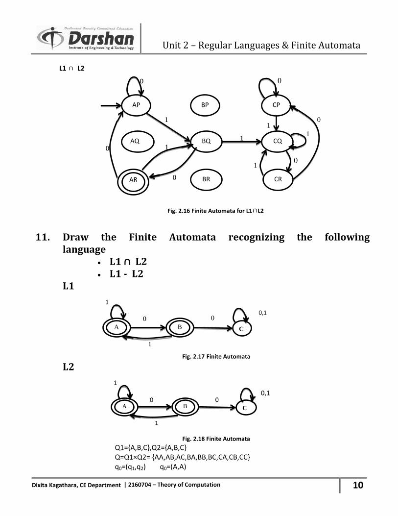
L1 ∩ L2
11. Draw the Finite Automata recognizing the following language
L1 ∩ L2 L1 - L2
L1
Fig. 2.17 Finite Automata
L2
Fig. 2.18 Finite Automata
Q1={A,B,C},Q2={A,B,C} Q=Q1×Q2= {AA,AB,AC,BA,BB,BC,CA,CB,CC} q0=(q1,q2) q0=(A,A)
0,1 0 0
1
A B
1
C
0,1 0 0
1
A B
1
C
1
AP
0 AQ
BP
BQ
BR
CP
CQ 1
1
0
1
0
1 0
1
0
0
AR CR
Fig. 2.16 Finite Automata for L1∩L2
Unit 2 – Regular Languages & Finite Automata
11
Dixita Kagathara, CE Department | 2160704 – Theory of Computation
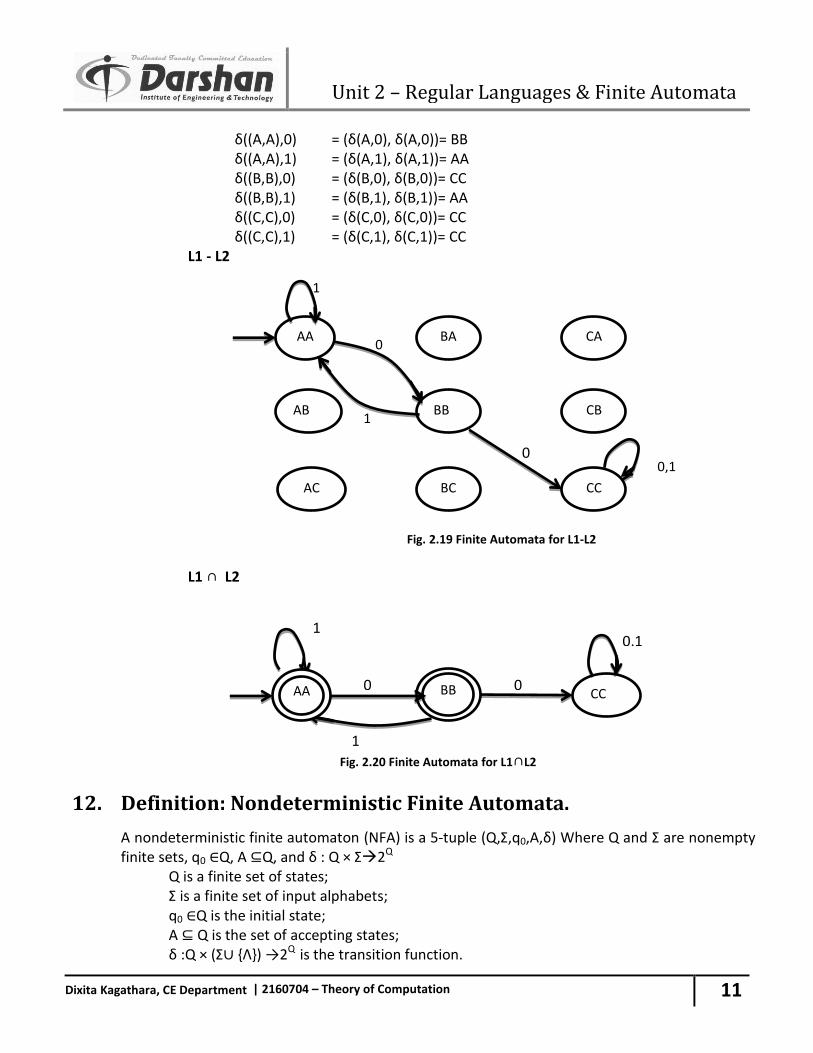
δ((A,A),0) = (δ(A,0), δ(A,0))= BB δ((A,A),1) = (δ(A,1), δ(A,1))= AA δ((B,B),0) = (δ(B,0), δ(B,0))= CC δ((B,B),1) = (δ(B,1), δ(B,1))= AA δ((C,C),0) = (δ(C,0), δ(C,0))= CC δ((C,C),1) = (δ(C,1), δ(C,1))= CC L1 - L2
Fig. 2.19 Finite Automata for L1-L2
L1 ∩ L2
Fig. 2.20 Finite Automata for L1∩L2
12. Definition: Nondeterministic Finite Automata.
A nondeterministic finite automaton (NFA) is a 5-tuple (Q,Ʃ,q0,A,δ) Where Q and Ʃ are nonempty finite sets, q0 ∈Q, A ⊆Q, and δ : Q × Ʃ2Q Q is a finite set of states; Ʃ is a finite set of input alphabets; q0 ∈Q is the initial state; A ⊆ Q is the set of accepting states; δ :Q × (Ʃ∪ {Λ}) →2Q is the transition function.
0,1
0 AA
AB
0
AC
1
BA
BB
BC
CA
CB
1
CC
0
1
0,1 1
0 BB CC
AA
Unit 2 – Regular Languages & Finite Automata
12
Dixita Kagathara, CE Department | 2160704 – Theory of Computation
13. Definition: Non recursive Definition of δ* for an NFA.
For an NFA M=(Q,Ʃ, q0,A, δ), and any p ∈ Q, δ*(p, Λ)= {p}. For any p ∈ Q and x= a1a2….an ∈ Ʃ* (with n≥1), δ*(p ,x) is the set of all states q for which there is a sequence of states p=p0,p1,….pn-
1,pn = q satisfying Pi ∈δ (pi-1 , ai) for each i with1 ≤ i ≤ n
14. Definition: Recursive Definition of δ* for an NFA
Let M=(Q,Ʃ, q0,A, δ), be an NFA. The function δ*: Q × Ʃ* 2Q is defined as follows. 1) For any q ∈ Q, δ*(q, Λ) = {q}. 2) For any q ∈ Q, y ∈Ʃ*, and a ∈Ʃ,
δ*(q, ya)= U δ(r, a) r ∈δ*(q, y)
15. Definition: Acceptance by an NFA Let M= (Q,Ʃ,q0,A,δ) be an NFA. The string x ∈Ʃ* is accepted by M if δ*(q0, x) ∩ A≠Ø. The language
recognized, or accepted, by M is the set L(M) of all string accepted by M. For any language L ⊆ Ʃ*, L is recognized by M if L= L(M).
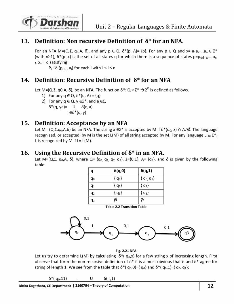
16. Using the Recursive Definition of δ* in an NFA. Let M=(Q,Ʃ, q0,A, δ), where Q= {q0, q1, q2, q3}, Ʃ={0,1}, A= {q3}, and δ is given by the following
table:
q δ(q,0) δ(q,1)
q0 { q0} { q0, q1}
q1 { q2} { q2}
q2 { q3} { q3}
q3 Ø Ø
Table 2.2 Transition Table
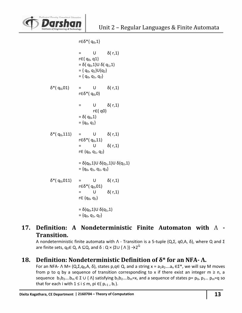
Fig. 2.21 NFA Let us try to determine L(M) by calculating δ*( q0,x) for a few string x of increasing length. First observe that form the non recursive definition of δ* it is almost obvious that δ and δ* agree for string of length 1. We see from the table that δ*( q0,0)={ q0} and δ*( q0,1)={ q0, q1}; δ*( q0,11) = U δ( r,1)
q0 q1 q
2 q3
0,1
0,1 0,1 1
Unit 2 – Regular Languages & Finite Automata
13
Dixita Kagathara, CE Department | 2160704 – Theory of Computation
r∈δ*{ q0,1} = U δ( r,1) r∈{ q0, q1} = δ{ q0,1}U δ( q1,1) = { q0, q1}U{q2} = { q0, q1, q2} δ*( q0,01) = U δ( r,1) r∈δ*( q0,0) = U δ( r,1) r∈( q0) = δ( q0,1) = {q0, q1} δ*( q0,111) = U δ( r,1) r∈δ*( q0,11) = U δ( r,1) r∈ (q0, q1, q2) = δ(q0,1)U δ(q1,1)U δ(q2,1) = {q0, q1, q2, q3} δ*( q0,011) = U δ( r,1) r∈δ*( q0,01) = U δ( r,1) r∈ (q0, q1) = δ(q0,1)U δ(q1,1) = {q0, q1, q2}
17. Definition: A Nondeterministic Finite Automaton with Λ - Transition.
A nondeterministic finite automata with Λ - Transition is a 5-tuple (Q,Ʃ, q0,A, δ), where Q and Ʃ are finite sets, q0∈ Q, A ⊆Q, and δ : Q × (Ʃ∪ { Λ }) →2Q
18. Definition: Nondeterministic Definition of δ* for an NFA- Λ. For an NFA- Λ M= (Q,Ʃ,q0,A, δ), states p,q∈ Q, and a string x = a1a2….an ∈Ʃ*, we will say M moves
from p to q by a sequence of transition corresponding to x if there exist an integer m ≥ n, a sequence b1b2….bm ∈ Ʃ ∪ { Λ} satisfying b1b2….bm=x, and a sequence of states p= p0, p1… pm=q so that for each i with 1 ≤ i ≤ m, pi ∈( pi-1 , bi ).
Unit 2 – Regular Languages & Finite Automata
14
Dixita Kagathara, CE Department | 2160704 – Theory of Computation
For x ∈ Ʃ* and p ∈δ*( p, x) is the set of all states q ∈ Q such that there is a sequence of transition corresponding to x by which M moves from p to q.
19. Definition: Λ- Closure of a Set of States. Let M=(Q,Ʃ, q0,A, δ), be an NFA – Λ, and let S ne any subset of Q. The Λ- closure of S is the set Λ(s)
defined as follows. 1) Every element of S is an element of Λ(s); 2) For any q ∈ Λ(s), every element of δ(q, Λ) is in Λ(s); 3) No other elements of Q are in Λ(s);
20. Definition: Recursive Definition of δ* for an NFA- Λ. Let M= (Q, Ʃ, q0, A, δ) be an NFA – Λ, The extended transition function δ*: Q × Ʃ*→2Q is defined
as follows. 1) For any q ∈ Q, δ*(q, Λ) = Λ({q}). 2) For any q ∈ Q, y ∈Ʃ*, and a∈ Λ,
δ*(q,ya)= Λ( U δ(r,a)) r∈ δ*(q,y)
A string x is accepted by M if δ*(q0, x) ∩ A ≠ Ø. The language recognized by M is the set L(M) of all strings accepted by M.
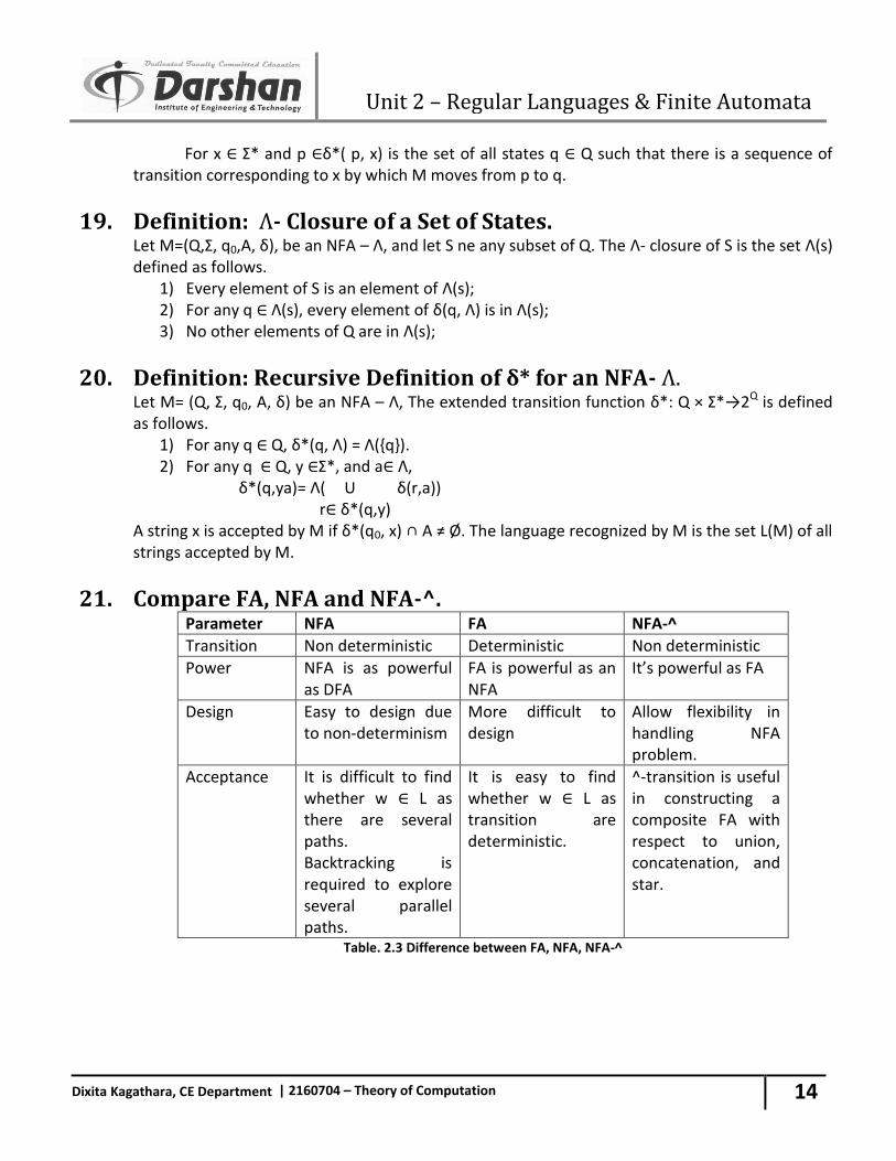
21. Compare FA, NFA and NFA-^. Parameter NFA FA NFA-^
Transition Non deterministic Deterministic Non deterministic
Power NFA is as powerful as DFA
FA is powerful as an NFA
It’s powerful as FA
Design Easy to design due to non-determinism
More difficult to design
Allow flexibility in handling NFA problem.
Acceptance It is difficult to find whether w ∈ L as there are several paths. Backtracking is required to explore several parallel paths.
It is easy to find whether w ∈ L as transition are deterministic.
^-transition is useful in constructing a composite FA with respect to union, concatenation, and star.
Table. 2.3 Difference between FA, NFA, NFA-^
Unit 2 – Regular Languages & Finite Automata
15
Dixita Kagathara, CE Department | 2160704 – Theory of Computation
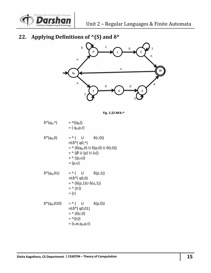
22. Applying Definitions of ^(S) and δ*
Fig. 2.22 NFA-^ δ*(q0,^) = ^({q0}) = { q0,p,t} δ*(q0,0) = ^ ( U δ(r,0)) r∈δ*( q0,^) = ^ (δ(q0,0) U δ(p,0) U δ(t,0)) = ^ (Ø U {p} U {u}) = ^ ({p,u}) = {p,u} δ*(q0,01) = ^ ( U δ(p,1)) r∈δ*( q0,0) = ^ (δ(p,1)U δ(u,1)) = ^ ({r}) = {r} δ*(q0,010) = ^ ( U δ(p,0)) r∈δ*( q0,01) = ^ (δ(r,0) = ^({s}) = {s,w,q0,p,t}
q0
P
t
r
u
S
v
W
^
0 1
^ ^
^ 0 0
0
^
1
0
1
Unit 2 – Regular Languages & Finite Automata
16
Dixita Kagathara, CE Department | 2160704 – Theory of Computation
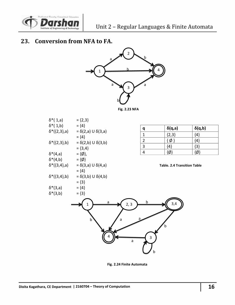
23. Conversion from NFA to FA.
Fig. 2.23 NFA δ*( 1,a) = {2,3} δ*( 1,b) = {4} δ*({2,3},a) = δ(2,a) U δ(3,a) = {4} δ*({2,3},b) = δ(2,b) U δ(3,b) = {3,4} δ*(4,a) = {Ø}, δ*(4,b) = {Ø} δ*({3,4},a) = δ(3,a) U δ(4,a) Table. 2.4 Transition Table = {4} δ*({3,4},b) = δ(3,b) U δ(4,b) = {3} δ*(3,a) = {4} δ*(3,b) = {3}
q δ(q,a) δ(q,b)
1 {2,3} {4}
2 { Ø } {4}
3 {4} {3}
4 {Ø} {Ø}
4 1
a
a
2
3
b
a
b
b
1 2, 3
3 4
a 3,4 b
a b a
a
b
b
Fig. 2.24 Finite Automata
Unit 2 – Regular Languages & Finite Automata
17
Dixita Kagathara, CE Department | 2160704 – Theory of Computation
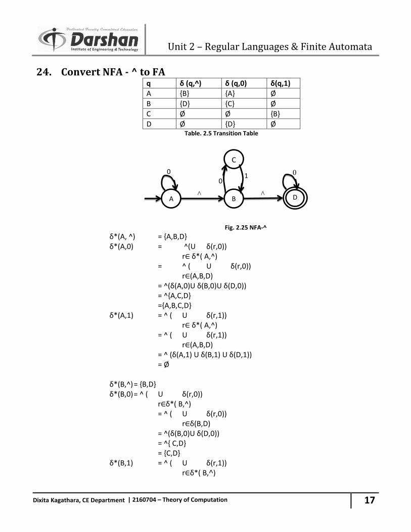
24. Convert NFA - ^ to FA q δ (q,^) δ (q,0) δ(q,1)
A {B} {A} Ø
B {D} {C} Ø
C Ø Ø {B}
D Ø {D} Ø Table. 2.5 Transition Table
Fig. 2.25 NFA-^
δ*(A, ^) = {A,B,D} δ*(A,0) = ^(U δ(r,0)) r∈ δ*( A,^) = ^ ( U δ(r,0)) r∈(A,B,D) = ^(δ(A,0)U δ(B,0)U δ(D,0)) = ^{A,C,D} ={A,B,C,D} δ*(A,1) = ^ ( U δ(r,1)) r∈ δ*( A,^) = ^ ( U δ(r,1)) r∈(A,B,D) = ^ (δ(A,1) U δ(B,1) U δ(D,1)) = Ø δ*(B,^) = {B,D} δ*(B,0) = ^ ( U δ(r,0)) r∈δ*( B,^) = ^ ( U δ(r,0)) r∈δ(B,D) = ^(δ(B,0)U δ(D,0)) = ^{ C,D} = {C,D} δ*(B,1) = ^ ( U δ(r,1)) r∈δ*( B,˄)
0
A B D ^ ^
0
1
0
C
Unit 2 – Regular Languages & Finite Automata
18
Dixita Kagathara, CE Department | 2160704 – Theory of Computation
= ^ ( U δ(r,1)) r∈(B,D) = ^(δ(B,1)U δ(D,1)) = Ø δ*(C,˄) = {C} δ*(C,0) = ^ ( U δ(r,0)) r∈δ*( C,˄) = ^ ( U δ(r,0)) r∈(C) = ^(δ(C,0)) = Ø δ*(C,1) = ^ ( U δ(r,1)) r∈δ*( C,˄) = ^ ( U δ(r,1)) r∈(C) = ^(δ(C,1)) = ^{B} = {B,D} δ*(D,˄) = {D} δ*(D,0) = ^ ( U δ(r,0)) r∈δ*( D,^) = ^ ( U δ(r,0)) r∈(D) = ^(δ(D,0)) = {D} δ*(D,1) = ^ ( U δ(r,1)) r∈δ*( D,^) = ^ ( U δ(r,1)) r∈(D) = ^(δ(D,1)) = Ø
A
D B
A
C
0 0
0 1
0 0
0
0
1
Unit 2 – Regular Languages & Finite Automata
19
Dixita Kagathara, CE Department | 2160704 – Theory of Computation
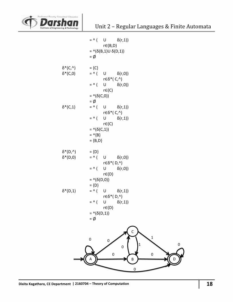
Fig. 2.26 NFA δ({A},0) = {A,B,C,D} δ({A},1) = Ø δ({A,B,C,D},0) = (δ(A,0) U δ(B,0) U δ(C,0) U δ(D,0)) = {A,B,C,D} δ({A,B,C,D},1) = (δ(A,1)U δ(B,1)U δ(C,1)U δ(D,1)) = {B,D} δ({B,D},0) = (δ(B,0)U δ(D,0)) = {C,D} δ({B,D},1) = (δ(B,1)U δ(D,1)) = Ø δ({C,D},0) = (δ(C,0)U δ(D,0)) = {D} δ({C,D},1) = (δ(C,1)U δ(D,1)) = {B,D} δ({D},0) = {D} δ({D},1) = Ø
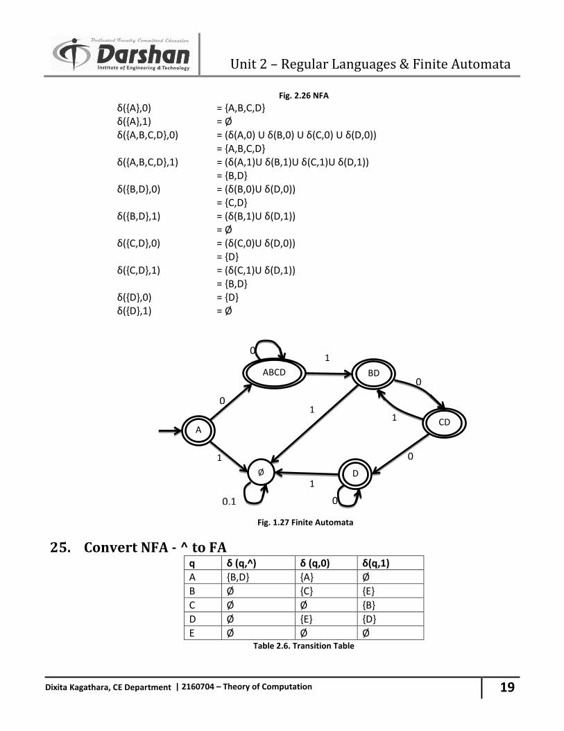
25. Convert NFA - ^ to FA q δ (q,^) δ (q,0) δ(q,1)
A {B,D} {A} Ø
B Ø {C} {E}
C Ø Ø {B}
D Ø {E} {D}
E Ø Ø Ø Table 2.6. Transition Table
A
BD
D
ABCD
1
Ø
CD
1
0
1
1
0
0
0,1 0
1
0
Fig. 1.27 Finite Automata
Unit 2 – Regular Languages & Finite Automata
20
Dixita Kagathara, CE Department | 2160704 – Theory of Computation
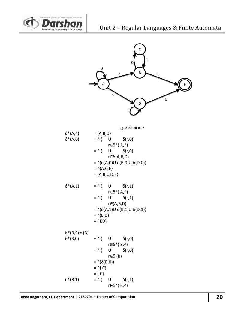
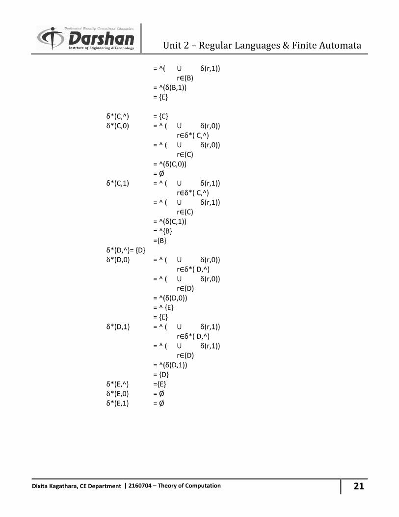
Fig. 2.28 NFA -^ δ*(A,^) = {A,B,D} δ*(A,0) = ^ ( U δ(r,0)) r∈δ*( A,^) = ^ ( U δ(r,0)) r∈δ(A,B,D) = ^(δ(A,0)U δ(B,0)U δ(D,0)) = ^{A,C,E} = {A,B,C,D,E} δ*(A,1) = ^ ( U δ(r,1)) r∈δ*( A,^) = ^ ( U δ(r,1)) r∈(A,B,D) = ^(δ(A,1)U δ(B,1)U δ(D,1)) = ^(E,D) = { ED} δ*(B,^) = {B} δ*(B,0) = ^ ( U δ(r,0)) r∈δ*( B,^) = ^ ( U δ(r,0)) r∈δ (B) = ^(δ(B,0)) = ^{ C} = { C} δ*(B,1) = ^ ( U δ(r,1)) r∈δ*( B,^)
C
B
A
D
E
^
^
0
0
1
0
1
1
Unit 2 – Regular Languages & Finite Automata
21
Dixita Kagathara, CE Department | 2160704 – Theory of Computation
= ^( U δ(r,1)) r∈(B) = ^(δ(B,1)) = {E} δ*(C,^) = {C} δ*(C,0) = ^ ( U δ(r,0)) r∈δ*( C,^) = ^ ( U δ(r,0)) r∈(C) = ^(δ(C,0)) = Ø δ*(C,1) = ^ ( U δ(r,1)) r∈δ*( C,^) = ^ ( U δ(r,1)) r∈(C) = ^(δ(C,1)) = ^{B} ={B} δ*(D,^) = {D} δ*(D,0) = ^ ( U δ(r,0)) r∈δ*( D,^) = ^ ( U δ(r,0)) r∈(D) = ^(δ(D,0)) = ^ {E} = {E} δ*(D,1) = ^ ( U δ(r,1)) r∈δ*( D,^) = ^ ( U δ(r,1)) r∈(D) = ^(δ(D,1)) = {D} δ*(E,^) ={E} δ*(E,0) = Ø δ*(E,1) = Ø
Unit 2 – Regular Languages & Finite Automata
22
Dixita Kagathara, CE Department | 2160704 – Theory of Computation
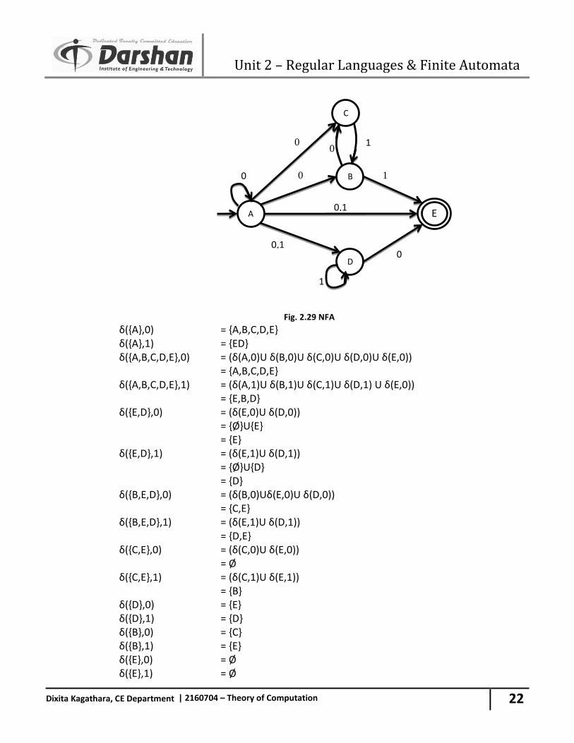
Fig. 2.29 NFA δ({A},0) = {A,B,C,D,E} δ({A},1) = {ED} δ({A,B,C,D,E},0) = (δ(A,0)U δ(B,0)U δ(C,0)U δ(D,0)U δ(E,0)) = {A,B,C,D,E} δ({A,B,C,D,E},1) = (δ(A,1)U δ(B,1)U δ(C,1)U δ(D,1) U δ(E,0)) = {E,B,D} δ({E,D},0) = (δ(E,0)U δ(D,0)) = {Ø}U{E} = {E} δ({E,D},1) = (δ(E,1)U δ(D,1)) = {Ø}U{D} = {D} δ({B,E,D},0) = (δ(B,0)Uδ(E,0)U δ(D,0)) = {C,E} δ({B,E,D},1) = (δ(E,1)U δ(D,1)) = {D,E} δ({C,E},0) = (δ(C,0)U δ(E,0)) = Ø δ({C,E},1) = (δ(C,1)U δ(E,1)) = {B} δ({D},0) = {E} δ({D},1) = {D} δ({B},0) = {C} δ({B},1) = {E} δ({E},0) = Ø δ({E},1) = Ø
0
A
C
B
0
D
0,1 E
0 0,1
1
0
0
1
1
Unit 2 – Regular Languages & Finite Automata
23
Dixita Kagathara, CE Department | 2160704 – Theory of Computation
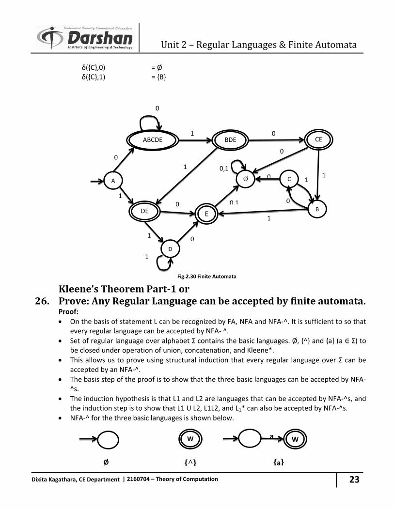
δ({C},0) = Ø δ({C},1) = {B}
26.
Kleene’s Theorem Part-1 or Prove: Any Regular Language can be accepted by finite automata.
Proof:
On the basis of statement L can be recognized by FA, NFA and NFA-^. It is sufficient to so that every regular language can be accepted by NFA- ^.
Set of regular language over alphabet Ʃ contains the basic languages. Ø, {^} and {a} (a ∈ Ʃ) to be closed under operation of union, concatenation, and Kleene*.
This allows us to prove using structural induction that every regular language over Ʃ can be accepted by an NFA-^.
The basis step of the proof is to show that the three basic languages can be accepted by NFA-^s.
The induction hypothesis is that L1 and L2 are languages that can be accepted by NFA-^s, and the induction step is to show that L1 U L2, L1L2, and L1* can also be accepted by NFA-^s.
NFA-^ for the three basic languages is shown below.
a W W
Ø {^} {a}
1
ABCDE
A
E
D
BDE CE
Ø
B
0
0
C
DE
1 0
1 1
0,1
1
0
0
1
0
0
1
0,1
0
1
Fig.2.30 Finite Automata
Unit 2 – Regular Languages & Finite Automata
24
Dixita Kagathara, CE Department | 2160704 – Theory of Computation
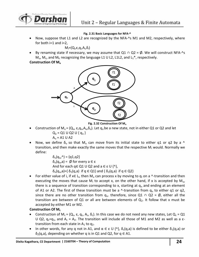
Fig. 2.31 Basic Languages for NFA-^ Now, suppose that L1 and L2 are recognized by the NFA-^s M1 and M2, respectively, where
for both i=1 and i=2, Mi=(Qi,ε,qi,Ai,δi)
By renaming state if necessary, we may assume that Q1 ∩ Q2 = Ø. We will construct NFA-^s Mu, Mc, and Mk recognizing the language L1 U L2, L1L2, and L1*, respectively.
Construction Of Mu
Fig. 2.32 Construction Of Mu
Construction of Mu = (Qu, ε,qu,Au,δu). Let qu be a new state, not in either Q1 or Q2 and let Qu = Q1 U Q2 U { qu } Au = A1 U A2
Now, we define δu so that Mu can move from its initial state to either q1 or q2 by a ^ transition, and then make exactly the same moves that the respective Mi would. Normally we define:
δu(qu,^) = {q1,q2} δu(qu,a) = Ø for every a ∈ ε And for each q∈ Q1 U Q2 and a ∈ ε U {^}, δu(qu,a)={ δ1(q,a) if q ∈ Q1} and { δ2(q,a) if q ∈ Q2}
For either value of i, if x∈ Li, then Mu can process x by moving to qi on a ^-transition and then executing the moves that cause Mi to accept x, on the other hand, if x is accepted by Mu, there is a sequence of transition corresponding to x, starting at qu and ending at an element of A1 or A2. The first of these transition must be a ^-transition from qu to either q1 or q2, since there are no other transition from qu. therefore, since Q1 ∩ Q2 = Ø, either all the transition are between of Q1 or all are between elements of Q2. It follow that x must be accepted by either M1 or M2.
Construction Of Mc
Construction of Mc = (Qc, ε, qc, Ac, δc). In this case we do not need any new states, Let Qc = Q1 U Q2, qc=q1, and Ac = A2. The transition will include all those of M1 and M2 as well as a ε-transition from each state in A1 to q2.
In other words, for any q not in A1, and α ∈ ε U {^}, δc(q,a) is defined to be either δ1(q,a) or δ2(q,a), depending on whether q is in Q1 and Q2, for q ∈ A1.
qu
q1
^ q2
^
f1
f1’
f2
f2’
Unit 2 – Regular Languages & Finite Automata
25
Dixita Kagathara, CE Department | 2160704 – Theory of Computation
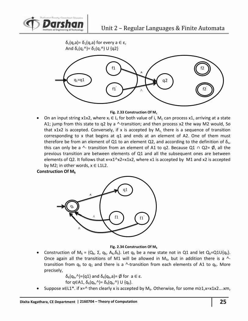
δc(q,a)= δ1(q,a) for every a ∈ ε, And δc(q,˄)= δ1(q,˄) U {q2}
Fig. 2.33 Construction Of Mc
On an input string x1x2, where xi ∈ Li for both value of i, Mc can process x1, arriving at a state A1; jump from this state to q2 by a ˄-transition; and then process x2 the way M2 would, So that x1x2 is accepted. Conversely, if x is accepted by Mc, there is a sequence of transition corresponding to x that begins at q1 and ends at an element of A2. One of them must therefore be from an element of Q1 to an element Q2, and according to the definition of δc, this can only be a ˄- transition from an element of A1 to q2. Because Q1 ∩ Q2= Ø, all the previous transition are between elements of Q1 and all the subsequent ones are between elements of Q2. It follows that x=x1˄x2=x1x2, where x1 is accepted by M1 and x2 is accepted by M2; in other words, x ∈ L1L2.
Construction Of Mk
Fig. 2.34 Construction Of Mk
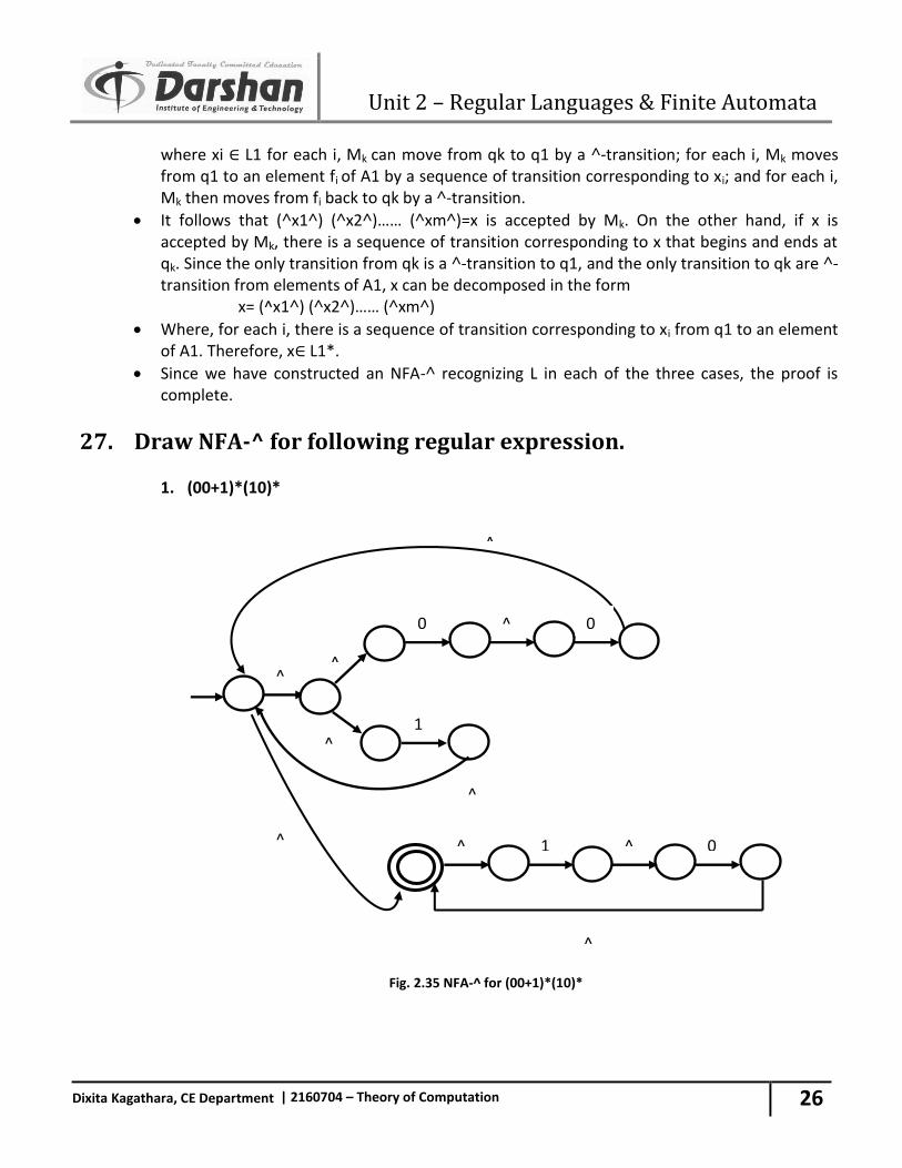
Construction of Mk = (Qk, Ʃ, qk, Ak,δk). Let qk be a new state not in Q1 and let Qk=Q1U{qk}. Once again all the transitions of M1 will be allowed in Mk, but in addition there is a ˄-transition from qk to q1 and there is a ˄-transition from each elements of A1 to qk. More precisely,
δk(qk,˄)={q1} and δk(qk,a)= Ø for a ∈ ε. for q∈A1, δk(qk,˄)= δk(qk,˄) U {qk}.
Suppose x∈L1*. if x=˄ then clearly x is accepted by Mk. Otherwise, for some m≥1,x=x1x2….xm,
^
qk
q1
1
f1
^
^
f1’
^
qc=q1
^
f1
f1’
f2
f2’
q2
Unit 2 – Regular Languages & Finite Automata
26
Dixita Kagathara, CE Department | 2160704 – Theory of Computation
where xi ∈ L1 for each i, Mk can move from qk to q1 by a ˄-transition; for each i, Mk moves from q1 to an element fi of A1 by a sequence of transition corresponding to xi; and for each i, Mk then moves from fi back to qk by a ˄-transition.
It follows that (˄x1˄) (˄x2˄)…… (˄xm˄)=x is accepted by Mk. On the other hand, if x is accepted by Mk, there is a sequence of transition corresponding to x that begins and ends at qk. Since the only transition from qk is a ˄-transition to q1, and the only transition to qk are ˄-transition from elements of A1, x can be decomposed in the form
x= (^x1˄) (˄x2˄)…… (˄xm˄)
Where, for each i, there is a sequence of transition corresponding to xi from q1 to an element of A1. Therefore, x∈ L1*.
Since we have constructed an NFA-˄ recognizing L in each of the three cases, the proof is complete.
27. Draw NFA-^ for following regular expression.
1. (00+1)*(10)*
Fig. 2.35 NFA-^ for (00+1)*(10)*
^
^
^ 0
1
0
^
^
0 ^ 1 ^ ^
^
^
Unit 2 – Regular Languages & Finite Automata
27
Dixita Kagathara, CE Department | 2160704 – Theory of Computation
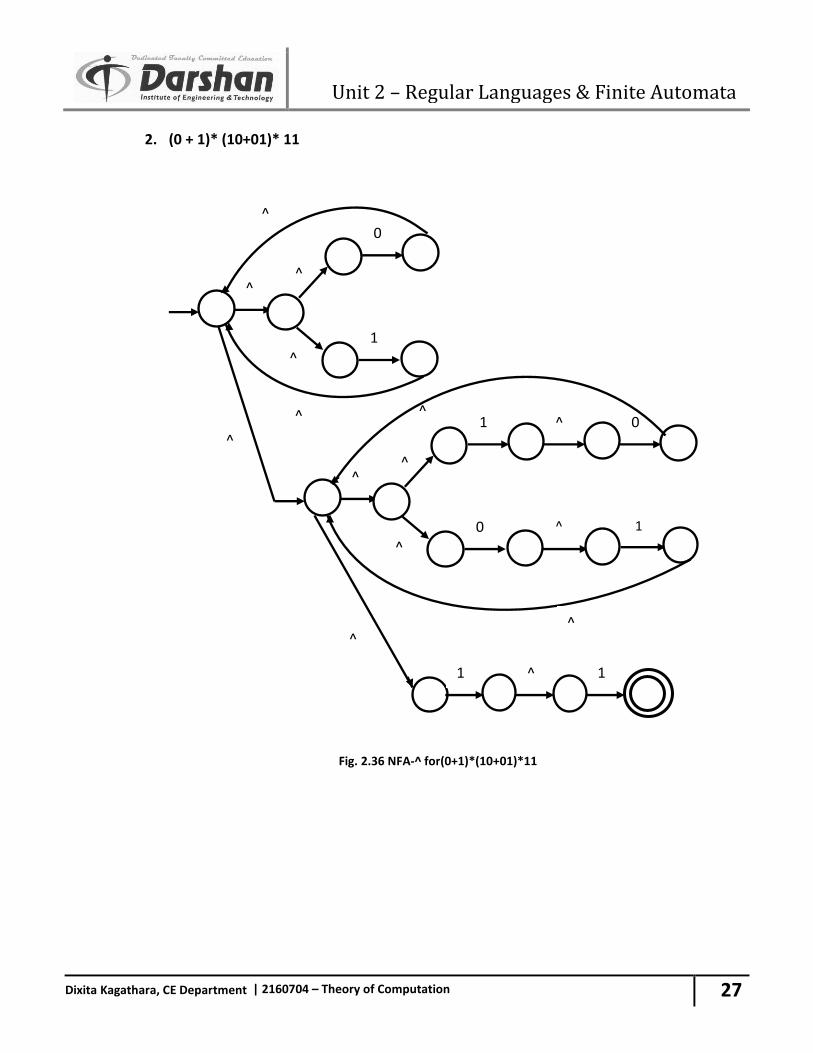
2. (0 + 1)* (10+01)* 11
Fig. 2.36 NFA-^ for(0+1)*(10+01)*11
^
0
1
^
^
1 ^ 1
^
^
^ 1
0
0
^
^
^ ^
^
^
^
1 ^
Unit 2 – Regular Languages & Finite Automata
28
Dixita Kagathara, CE Department | 2160704 – Theory of Computation
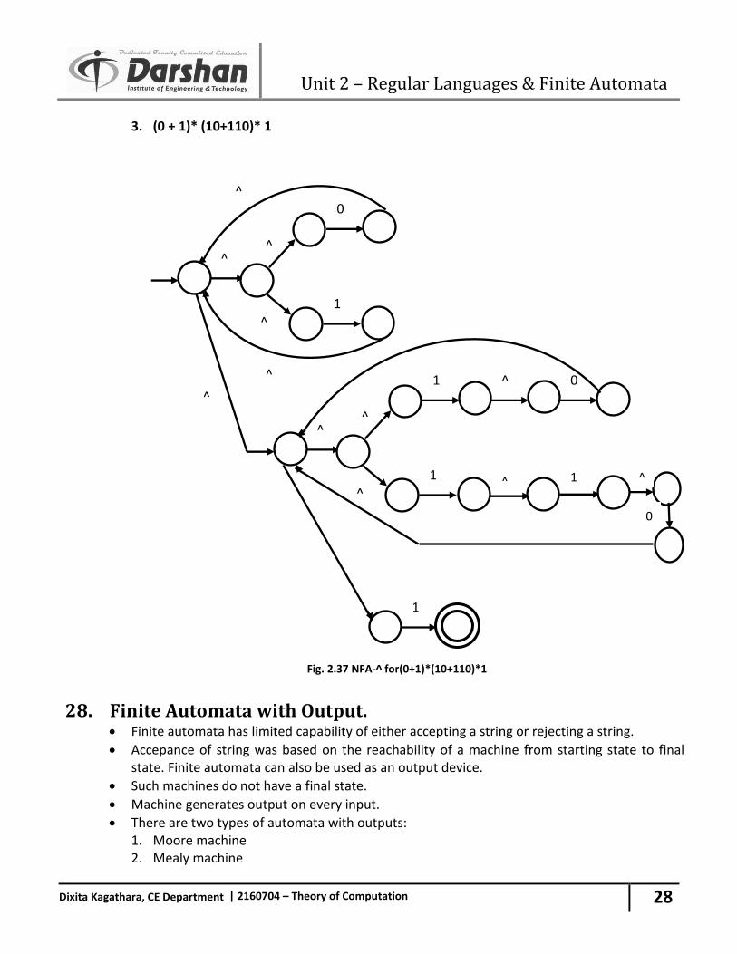
3. (0 + 1)* (10+110)* 1
Fig. 2.37 NFA-^ for(0+1)*(10+110)*1
28. Finite Automata with Output. Finite automata has limited capability of either accepting a string or rejecting a string.
Accepance of string was based on the reachability of a machine from starting state to final state. Finite automata can also be used as an output device.
Such machines do not have a final state.
Machine generates output on every input.
There are two types of automata with outputs: 1. Moore machine 2. Mealy machine
^
0
1
^
^
^
^ 1
1
0
^
^
^
^
^
1
^
0 0
^
^ 1
Unit 2 – Regular Languages & Finite Automata
29
Dixita Kagathara, CE Department | 2160704 – Theory of Computation
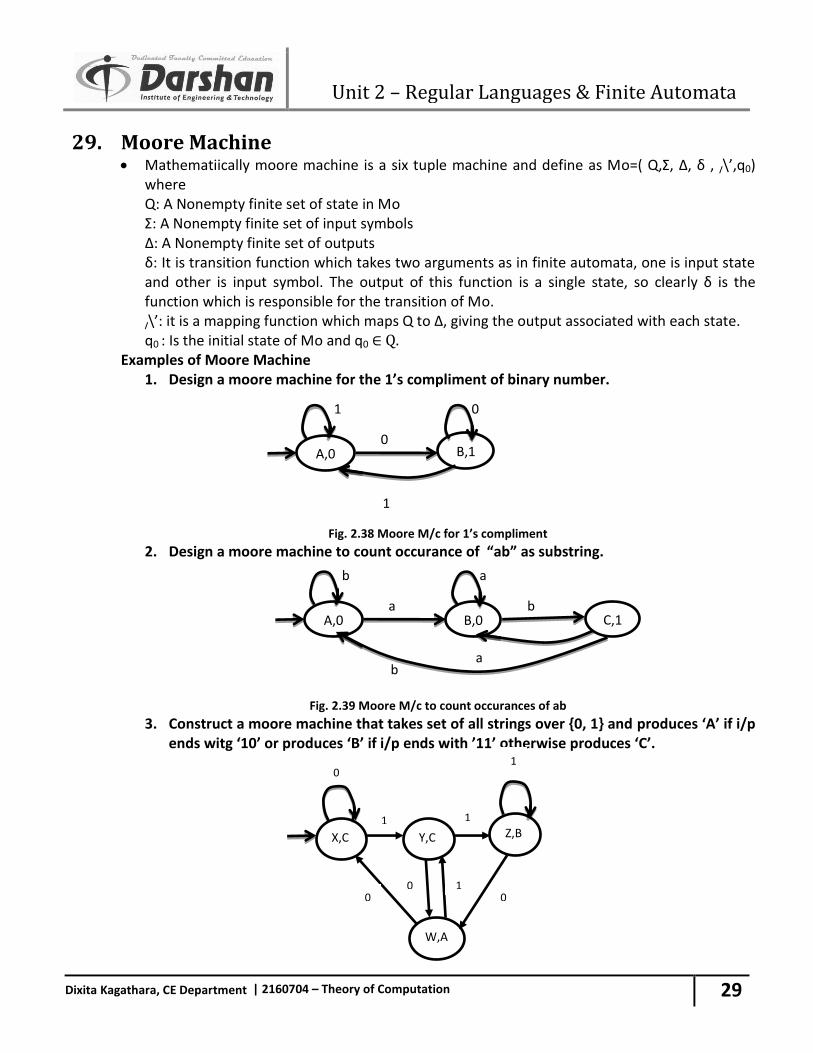
29. Moore Machine Mathematiically moore machine is a six tuple machine and define as Mo=( Q,Ʃ, ∆, δ , /\’,q0)
where Q: A Nonempty finite set of state in Mo Ʃ: A Nonempty finite set of input symbols ∆: A Nonempty finite set of outputs δ: It is transition function which takes two arguments as in finite automata, one is input state and other is input symbol. The output of this function is a single state, so clearly δ is the function which is responsible for the transition of Mo.
/\’: it is a mapping function which maps Q to ∆, giving the output associated with each state. q0 : Is the initial state of Mo and q0 ∈ Q.
Examples of Moore Machine 1. Design a moore machine for the 1’s compliment of binary number.
Fig. 2.38 Moore M/c for 1’s compliment
2. Design a moore machine to count occurance of “ab” as substring.
Fig. 2.39 Moore M/c to count occurances of ab 3. Construct a moore machine that takes set of all strings over {0, 1} and produces ‘A’ if i/p
ends witg ‘10’ or produces ‘B’ if i/p ends with ’11’ otherwise produces ‘C’.
b
A,0 b
B,0 a
b a
a
C,1
1
A,0 B,1 0
1 0
X,C Y,C Z,B
W,A
AA
0
1
1 1
0 0 1 0
Unit 2 – Regular Languages & Finite Automata
30
Dixita Kagathara, CE Department | 2160704 – Theory of Computation
Fig. 2.40 Moore M/c for string ending in 10 or 11
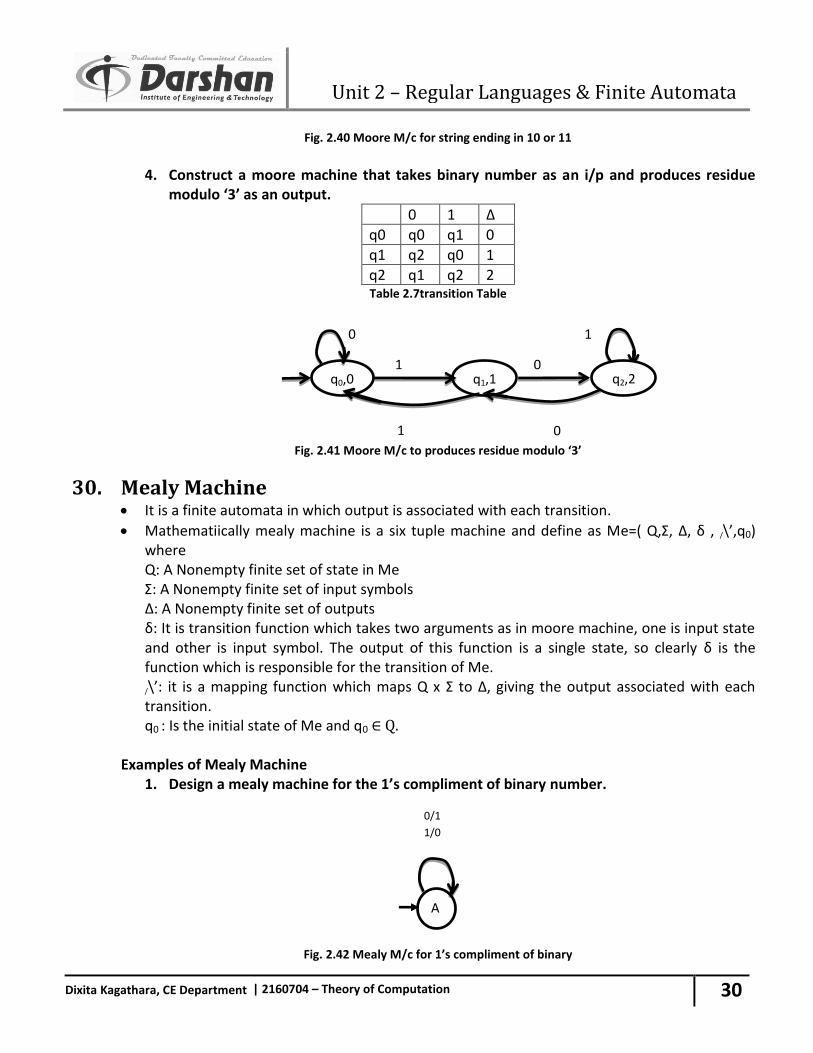
4. Construct a moore machine that takes binary number as an i/p and produces residue modulo ‘3’ as an output.
0 1 ∆
q0 q0 q1 0
q1 q2 q0 1
q2 q1 q2 2 Table 2.7transition Table
Fig. 2.41 Moore M/c to produces residue modulo ‘3’
30. Mealy Machine It is a finite automata in which output is associated with each transition.
Mathematiically mealy machine is a six tuple machine and define as Me=( Q,Ʃ, ∆, δ , /\’,q0) where Q: A Nonempty finite set of state in Me Ʃ: A Nonempty finite set of input symbols ∆: A Nonempty finite set of outputs δ: It is transition function which takes two arguments as in moore machine, one is input state and other is input symbol. The output of this function is a single state, so clearly δ is the function which is responsible for the transition of Me.
/\’: it is a mapping function which maps Q x Ʃ to ∆, giving the output associated with each transition. q0 : Is the initial state of Me and q0 ∈ Q.
Examples of Mealy Machine
1. Design a mealy machine for the 1’s compliment of binary number.
Fig. 2.42 Mealy M/c for 1’s compliment of binary
1
q0,0 0
q1,1 1
0 1
0
q2,2
A
0/1
1/0
Unit 2 – Regular Languages & Finite Automata
31
Dixita Kagathara, CE Department | 2160704 – Theory of Computation
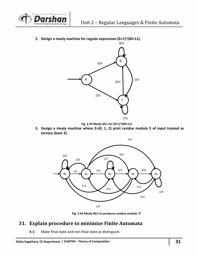
2. Design a mealy machine for regular expression (0+1)*(00+11).
Fig. 2.43 Mealy M/c for (0+1)*(00+11)
3. Design a mealy machine where Ʃ={0, 1, 2} print residue modulo 5 of input treated as ternary (base 3).
Fig. 2.44 Mealy M/c to produces residue modulo ‘5’
31. Explain procedure to minimize Finite Automata
S-1: Make final state and non-final state as distinguish.
1/n
0/n 1/n
0/n
0/x
1/y
A
B
C
1/4
0/0
1/1 0/1 2/3 0/4
0/3
2/2
1/0
0/2
1/3
2/0 1/2
2/4
2/1
q0 q1 q2 q3 q4
Unit 2 – Regular Languages & Finite Automata
32
Dixita Kagathara, CE Department | 2160704 – Theory of Computation
S-2: Recursively interacting over the pairs of state for any transition for δ(p,x) = r δ(q,x) = s and for x ∈ ε. If r and s are distinguishable make p and q as distinguish. S-3: If any iteration over all possible state pairs one fails to find a new pair of states that are distinguishable terminate. S-4: All the states that are not distinguished are equivalence.
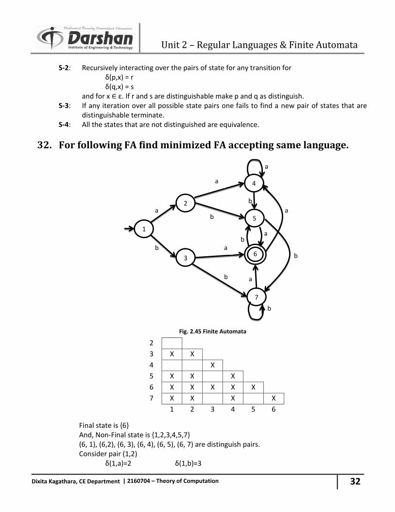
32. For following FA find minimized FA accepting same language.
Fig. 2.45 Finite Automata
Final state is {6} And, Non-Final state is {1,2,3,4,5,7} (6, 1), (6,2), (6, 3), (6, 4), (6, 5), (6, 7) are distinguish pairs.
Consider pair (1,2) δ(1,a)=2 δ(1,b)=3
2
3 X X
4 X
5 X X X
6 X X X X X
7 X X X X
1 2 3 4 5 6
1
b
b
4
5
3
7
a
6
a
b
b
a
a
a
b
b a
a
b
2
Unit 2 – Regular Languages & Finite Automata
33
Dixita Kagathara, CE Department | 2160704 – Theory of Computation
δ(2,a)=4 δ(2,b)=5 Consider pair (1,3) δ(1,a)=2 δ(1,b)=3 δ(3,a)=6 δ(3,b)=7 pair (2,6) is distinguish, so It’s a distinguished pair. Consider pair (1,4) δ(1,a)=2 δ(1,b)=3 δ(4,a)=4 δ(4,b)=5 Consider pair (1,5) δ(1,a)=2 δ(1,b)=3 δ(5,a)=6 δ(5,b)=7 pair (2,6) is distinguish, so It’s a distinguished pair. Consider pair (1,7) δ(1,a)=2 δ(1,b)=3 δ(7,a)=6 δ(7,b)=7 pair (2,6) is distinguish, so It’s a distinguished pair. Consider pair (2,3) δ(2,a)=4 δ(2,b)=5 δ3(,a)=6 δ(3,b)=7 pair (4,6) is distinguish, so It’s a distinguished pair. Consider pair (2,4) δ(2,a)=4 δ(2,b)=5 δ(4,a)=4 δ(4,b)=5 Consider pair (2,5) δ(2,a)=4 δ(2,b)=5 δ(5,a)=6 δ(5,b)=7 pair (4,6) is distinguish, so It’s a distinguished pair. Consider pair (2,7) δ(2,a)=4 δ(2,b)=5 δ(7,a)=6 δ(7,b)=7 pair (4,6) is distinguish, so It’s a distinguished pair. Consider pair (3,4) δ(3,a)=6 δ(3,b)=7 δ(4,a)=4 δ(4,b)=5 pair (6,4) is distinguish, so (3,4) is distinguish. Consider pair (3,5) δ(3,a)=6 δ(3,b)=7 δ(5,a)=6 δ(5,b)=7 Consider pair (3,7) δ(3,a)=6 δ(3,b)=7 δ(7,a)=6 δ(7,b)=7 Consider pair (4,5) δ(4,a)=4 δ(4,b)=5
Unit 2 – Regular Languages & Finite Automata
34
Dixita Kagathara, CE Department | 2160704 – Theory of Computation
δ(5,a)=6 δ(5,b)=7 pair (6,4) is distinguish, so (4,5) is distinguish. Consider pair (4,7) δ(4,a)=4 δ(4,b)=5 δ(7,a)=6 δ(7,b)=7 pair (6,4) is distinguish, so (4,7) is distinguish. Consider pair (5,7) δ(5,a)=6 δ(5,b)=7 δ(7,a)=6 δ(7,b)=7
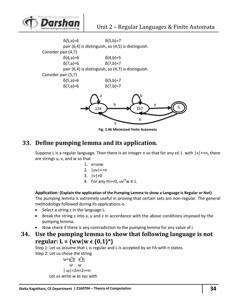
Fig. 2.46 Minimized Finite Automata
33. Define pumping lemma and its application.
Suppose L is a regular language. Then there is an integer n so that for any x∈ L with |x|>=n, there are strings u, v, and w so that
1. x=uvw 2. |uv|<=n 3. |v|>0 4. For any m>=0, uvmw ∈ L
Application: (Explain the application of the Pumping Lemma to show a Language is Regular or Not) The pumping lemma is extremely useful in proving that certain sets are non-regular. The general methodology followed during its applications is :
Select a string z in the language L.
Break the string z into x, y and z in accordance with the above conditions imposed by the pumping lemma.
Now check if there is any contradiction to the pumping lemma for any value of i.
34. Use the pumping lemma to show that following language is not regular: L = {ww|w ϵ {0,1}*}
Step 1: Let us assume that L is regular and L is accepted by an FA with n states. Step 2: Let us chose the string ῳ=anb anb
ῳ ῳ
| ῳ|=2n+2>=n Let us write w as xyz with
a
124 a
357 6 b
a b
b
Unit 2 – Regular Languages & Finite Automata
35
Dixita Kagathara, CE Department | 2160704 – Theory of Computation
|y|>0 And |xy|<=n Since |xy|<=n, x must be of the form as. Since |xy|<=n, y must be of the form ar | r>0 Now ῳ=anbanb= as ar an-s-rbanb x y z Step 3: Let us check whether x yi z for i=2 belongs to L. Xy2z= as a2r an-s-rbanb= an+rbanb Since, r>0, an+rbanb is not of the form ῳῳ as the number of a’s in the first half is n+r and second half is n. Therefore, xy2z L. Hence by contrdiction we can say language is not regular.
35. Prove that the language L = {0n: n is a prime number} is not regular.
Step 1: Let us assume that L is regular and L is accepted by an FA with n states. Step 2: Let us chose the string ῳ=ap ,where p is prime and p>n | ῳ|= | ap| = p>=n Let us write w as xyz with |y|>0 And |xy|<=n Since |xy|<=n, x must be of the form as. We assume that y= am for m>0. Step 3: Length of x yi z can be written as given below. Xyiz= |xyz|+|yi-1|=p+(i-1)m As |y|=| am |=m Let us check whether P(i-1) m is prime for every i. For i=p+1, p+(i-1)m= P+ Pm =P(1+m) So xyp+1z L. Hence by contrdiction we can say language is not regular.
36. Use Pumping Lemma to show that following language is not regular. L = { wwR / w ε {0,1}* }
Step 1: Let us assume that L is regular and L is accepted by an FA with n states. Step 2: Let us chose the string ῳ=anb ban
ῳ ῳR
| ῳ|=2n+2>=n Let us write w as xyz with |y|>0 And |xy|<=n Since |xy|<=n, x must be of the form as. Since |xy|<=n, y must be of the form ar | r>0 Now ῳ=anbban= as ar an-s-rbban x y z
Unit 2 – Regular Languages & Finite Automata
36
Dixita Kagathara, CE Department | 2160704 – Theory of Computation
Step 3: Let us check whether x yi z for i=2 belongs to L. Xy2z= as a2r an-s-rbban= an+rbban Since, r>0, an+rbban is not of the form ῳῳR as the string starts with (n+r) a’s but ends in (n) a’s. Therefore, Xy2z L. Hence by contrdiction we can say language is not regular.
Unit 3 – Context Free Grammar
1
Dixita Kagathara, CE Department | 2160704 – Theory of Computation
1. Define: Context Free Grammar & Context Free Language. Context Free Grammar:
A context free grammar is a 4-tuple G=(V,Ʃ,S,P) where, V is finite set of non terminals, Ʃ is disjoint finite set of terminals, S is an element of V and it’s a start symbol, P is a finite set formulas of the form Aα where A ∈ V and α∈ (V U Ʃ)*. Application of Context Free Grammar(CFG):
1) CFG are extensively used to specify the syntax of programming language. 2) CFG is used to develop a parser.
Context Free Language: Language generated by CFG is called context free language. Let G= (V, Ʃ, S, P) be a CFG. The Language generated by G is L(G) : {x ∈Ʃ*/S⟹G* x} A language L is a context free Language(CFL) if, there is a CFG G so that L=L(G)
2. Define: Regular Grammar. A grammar G=(V,Ʃ,S,P) is regular if every production takes one of the two forms,
BaC Ba Where B and C are Nonterminals and a is terminal.
3. Give Recursive Definitions for following. I. Recursive Definition of {a,b}*
1. ˄∈L. 2. For any S∈L, Sa∈L. 3. For any S∈L, Sb∈L. 4. No other strings are in L.
II. Recursive Definition of Palindrome (pal) 1. ˄, a, b ∈ pal 2. For any S ∈ pal , aSa ∈ pal and bSb ∈ pal 3. No other string are in pal
III. The language {anbn / n≥0} 1. ˄∈ L 2. For every x ∈ L, axb ∈L 3. No other strings are in L
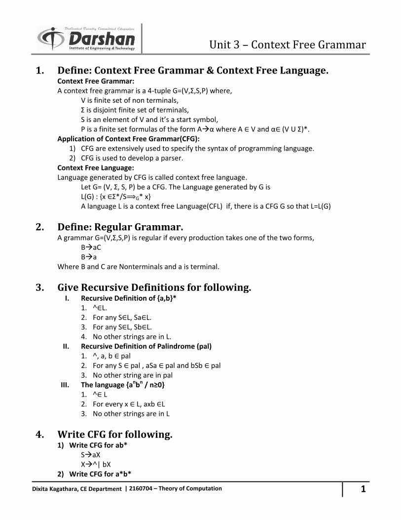
4. Write CFG for following. 1) Write CFG for ab*
SaX X˄| bX
2) Write CFG for a*b*
Unit 3 – Context Free Grammar
2
Dixita Kagathara, CE Department | 2160704 – Theory of Computation
SXY XaX|˄ YbY|˄
3) Write CFG for (011+1)*(01)* SAB A011A | 1A | ^ B01B | ^
4) Write CFG which contains at least three times 1. SA1A1A1A A0A | 1A | ^
5) Write CFG that must start and end with same symbol. S0A0 | 1A1
A0A | 1A | ^ 6) The language of even & odd length palindrome string over {a,b}
SaSa|bSb|a|b|˄ 7) No. of a and no. of b are same
SaSb|bSa|˄ 8) Write CFG for regular expression (a+b)*a(a+b)*a(a+b)* SXaXaX
XaX|bX|˄ 9) Write CFG for L={aibjck | i=j or j=k}
For i=j for j=k S->AB S->CD A->aAb | ab C->aC | a B->cB | c D->bDc | bc
10) Write CFG for L={ aibjck | j>i+k} SABC AaAb |˄ BbB | b CbCc |˄
11) Write CFG for L={ 0i1j0k | j>i+k} SABC A0A1 |˄ B1B | 1 C1C0 |˄
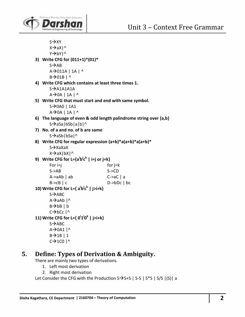
5. Define: Types of Derivation & Ambiguity. There are mainly two types of derivations.
1. Left most derivation 2. Right most derivation
Let Consider the CFG with the Production SS+S | S-S | S*S | S/S |(S)| a
Unit 3 – Context Free Grammar
3
Dixita Kagathara, CE Department | 2160704 – Theory of Computation
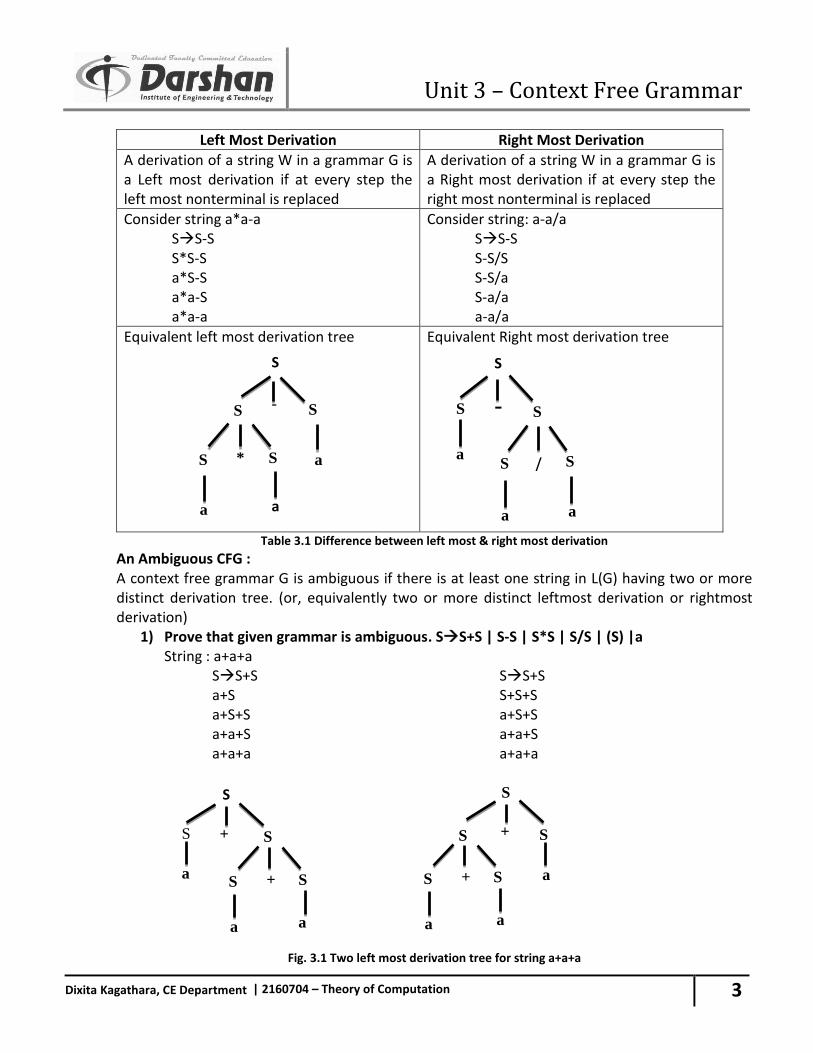
Left Most Derivation Right Most Derivation
A derivation of a string W in a grammar G is a Left most derivation if at every step the left most nonterminal is replaced
A derivation of a string W in a grammar G is a Right most derivation if at every step the right most nonterminal is replaced
Consider string a*a-a SS-S S*S-S a*S-S a*a-S a*a-a
Consider string: a-a/a SS-S
S-S/S S-S/a S-a/a a-a/a
Equivalent left most derivation tree
Equivalent Right most derivation tree
Table 3.1 Difference between left most & right most derivation
An Ambiguous CFG : A context free grammar G is ambiguous if there is at least one string in L(G) having two or more distinct derivation tree. (or, equivalently two or more distinct leftmost derivation or rightmost derivation)
1) Prove that given grammar is ambiguous. SS+S | S-S | S*S | S/S | (S) |a String : a+a+a
SS+S SS+S a+S S+S+S a+S+S a+S+S a+a+S a+a+S a+a+a a+a+a
Fig. 3.1 Two left most derivation tree for string a+a+a
S
S
S
S
+
a
S +
a
a
S
S
S
S +
a
S +
a
a
S
S
S
S
-
a
S /
a
a S
S S
S
-
a
S *
a
a
Unit 3 – Context Free Grammar
4
Dixita Kagathara, CE Department | 2160704 – Theory of Computation
Here, we have two left most derivation for string a+a+a hence, above grammar is ambiguous.
2) Prove that S->a | Sa | bSS | SSb | SbS is ambiguous String: baaab
SbSS SSSb baS bSSSb baSSb baSSb baaSb baaSb baaab baaab
We have two left most derivation for string baaab hence, above grammar is ambiguous.
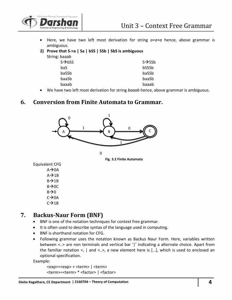
6. Conversion from Finite Automata to Grammar.
Fig. 3.2 Finite Automata
Equivalent CFG A0A A1B B1B B0C B0 C0A C1B
7. Backus-Naur Form (BNF) BNF is one of the notation techniques for context free grammar.
It is often used to describe syntax of the language used in computing.
BNF is shorthand notation for CFG.
Following grammar uses the notation known as Backus Naur Form. Here, variables written between <..> are non terminals and vertical bar ‘|’ indicating a alternate choice. Apart from the familiar notation =, | and <..>, a new element here is […], which is used to enclosed an optional specification.
Example: <exp>=<exp> + <term> | <term> <term>=<term> * <factor> | <factor>
A B 1
C 0
0 1
1
0
Unit 3 – Context Free Grammar
5
Dixita Kagathara, CE Department | 2160704 – Theory of Computation
<factor>=<factor> ^ <primary> | <primary> <primary>=<id> | <const> <id>=<letter> <const>=[+/-]<digit> <letter>=a | b | c |……| z <digit>=0 | 1 |………….| 9
8. Simplified forms & Normal forms. Definition: Nullable Variable
A Nullable variable in a CFG G=(V,Ʃ,S,P) is defined as follows: 1) Any variable A for which P contains A˄ is nullable. 2) if P contains production
AB1B2…..Bn where B1B2…Bn are nullable variable, then A is nullable. 3) No other variables in V are nullable.
Eliminate ˄ production : 1) SaX/Yb
XS/˄ YbY/b Grammar after elimination of ^ production: SaX/Yb/a
XS YbY/b
2) SXaX/bX/Y XXaX/XbX/˄ Yab Grammar after elimination of ^ production: SXaX/bX/Y/aX/Xa/a/b XXaX/aX/Xa/a/XbX/Xb/bX/b Yab
Definition: Unit Production Unit productions are always in the form of AB. Where A & B are single non terminals. Eliminate Unit Production:
1) SABA/BA/AA/AB/A/B AaA/a BbB/b Grammar after elimination of unit production: Unit production are SA and SB SABA/BA/AA/AB/aA/a/bB/b SaA/a SbB/b
2) SAa/B Aa/bc/B BA/bb
Unit 3 – Context Free Grammar
6
Dixita Kagathara, CE Department | 2160704 – Theory of Computation
Grammar after elimination of unit production: Unit production are SB,AB and BA. Aa/bc/B Aa/bc/A/bb Aa/bc/bb BA/bb Ba/bc/bb SAa/B SAa/a/bc/bb So CFG after removing unit production is: SAa/a/bc/bb Aa/bc/bb Ba/bc/bb
Definition: Chomsky Normal Form A context free grammar is in Chomsky normal form (CNF) is every production is one of these two forms: ABC Aa Where A, B, C are nonterminals and a is terminal. Step to convert CFG into CNF:
1) Eliminate ˄-Productions. 2) Eliminate Unit Productions. 3) Restricting the right side of productions to single terminal or string of two or more
nonterminals. (Replace all mixed string with solid NTs)
4) Final step of CNF. (shorten the string of NT to length 2)
9. Convert following CFG to CNF: SaX/Yb XS/˄ YbY/b
Step-1: Eliminate ˄-Production: Nullable production is X˄, new CFG without ˄-production is: SaX/a/Yb XS YbY/b Step-2: Eliminate Unit Production: Unit Production is XS, new CFG without Unit Production is: SaX/a/Yb
Unit 3 – Context Free Grammar
7
Dixita Kagathara, CE Department | 2160704 – Theory of Computation
XaX/a/Yb YbY/b Step-3: Replace all mixed string with solid NT: SAX/YB/a XAX/YB/a YBY/b Aa Bb Step-4 : Shorten the string of NT to length 2 All NT strings on the RHS in the above CFG are already the required length. So, CFG is in CNF.
10. Convert following CFG to CNF SAACD AaAb/˄ CaC/a DaDa/bDb/˄
Step-1: Eliminate ˄-Production: Nullable production is A˄ and D˄, new CFG without ˄-production is: apply for A˄ SAACD/ACD/CD Aab/aAb CaC/a DaDa/bDb/˄ apply for D˄ SAACD/ACD/CD/AAC/AC/C Aab/aAb CaC/a DaDa/bDb/aa/bb Step-2: Eliminate Unit Production: Unit Production is SC, new CFG without Unit Production is: SAACD/ACD/CD/AAC/AC/aC/a Aab/aAb CaC/a DaDa/bDb/aa/bb Step-3:Replace all mixed string with solid NT: SAACD/ACD/CD/AAC/AC/PC/a APQ/PAQ CPC/a DPDP/QDQ/PP/QQ Pa
Unit 3 – Context Free Grammar
8
Dixita Kagathara, CE Department | 2160704 – Theory of Computation
Qb Step-4 : Shorten the string of NT to length 2 SAT1, T1AT2 ,T2CD SAU1,U1CD SAV1,V1AC SCD/AC/PC/a APQ APW1, W1AQ CPC/a DPP/QQ DPY1, Y1DP DQZ1, Z1DQ Pa Qb
11. Convert following CFG to CNF SS(S)/˄
Step-1: Eliminate ˄-Production: Nullable production is S^, new CFG without ˄-production is: SS(S)/(S)/S()/() Step-2: Eliminate Unit Production: Here, there is no unit production, SS(S)/(S)/S()/() Step-3:Replace all mixed string with solid NT: SSXSY/XSY/SXY/XY X( Y) Step-4 : Shorten the string of NT to length 2 SST1, T1XT2, T2SY SXV1 V1SY SSU1 U1XY SXY X( Y)
12. Unions, Concatenations and Kleen’s of Context free language. Theorem:- If L1 and L2 are context - free languages, then the languages L1 U L2, L1L2 , and L1
* are also CFLs. The proof is constructive: Starting with CFGs
G1 = (V1, Ʃ, S1,P1) and G2 = (V2, Ʃ, S2,P2) , Generating L1 and L2, respectively, we show how to construct a new CFG for each of the three cases. A grammar Gu = (Vu, Ʃ, Su, Pu) generating L1 U L2. First we rename the element of V2 if necessary
Unit 3 – Context Free Grammar
9
Dixita Kagathara, CE Department | 2160704 – Theory of Computation
so that V1 ∩ V2= Ø and we define Vu= V1 U V2 U {Su} Where Su is a new symbol not in V1 or V2. Then we let Pu= P1 U P2 U { Su S1 | S2 }
On the one hand, if x is in either L1 or L2, then Su =>*x in the grammar Gu , because we can start a derivation with either Su S1 or Su S2 and continue with the derivation of x in G1
or G2 . Therefore, L1 U L2 ⊆ L(Gu) On the other hand, if x is derivable from Su in Gu, the first step in any derivation must be Su=>S1 or Su=>S2 In the first case, all subsequent productions used must be productions in G1 , because no variables in V2 are involved, and thus x∈ L1; in the second case, x ∈ L2. Therefore, L(Gu) ⊆ L1 U L2
A grammar Gc= (Vc, Ʃ, Sc, Pc) generating L1L2 . Again we relabel variables if necessary so that V1 ∩ V2 = Ø and define
Vc = V1 U V2 U {Sc} This time we let Pc= P1 U P2 U { ScS1S2 } If x ∈L1L2 then x = x1x2 , where xi ∈Li for each i. we may then derive x in Gc as follows: Sc =>S1 S2 => *x1 S2 => * x1x2 = x Where the second step is the derivation of x1 in G1 and the third step is the derivation of x2
in G2. Conversely, if x can be derived from Sc, then since the first step in the derivation must be Sc=>S1 S2 , x must be derivable from S1 S2. Therefore, x=x1x2, where for each i, xi can be derived from Si in Gc. Since V1 n V2 = Ø, being derivable from Si in Gc means being derivable from Si in Gi, and so x ∈ L1L2.
A grammar G* = (V, Ʃ, S, P) generating L1 *.Let V = V1 U {S} Where S V1.The language L1 *contains strings of the form x = x1x2 …xk , where each xi ∈ L1. Since each xi can be derived from S1, then to derive x from S it is enough to be able to derive a string of k S1‘S. We can accomplish this by including the productions
SS1S |
In P. Therefore, let
P = P1U { SS1S | } The proof that L1 * ⊆ L(G*) is straightforward. If x ∈ L(G*) , on the other hand, then either
x = or x can be derived from some string of the form S1k in G* . In the second case,
since the only production in G* beginning with S1 are those in G1, we may conclude that x∈ L(G1)k ⊆ L(G1)* .
Unit 4 – Pushdown Automata, CFL & NCFL
1
Dixita Kagathara, CE Department | 2160704 – Theory of Computation
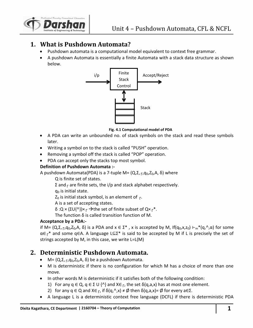
1. What is Pushdown Automata? Pushdown automata is a computational model equivalent to context free grammar.
A pushdown Automata is essentially a finite Automata with a stack data structure as shown below.
Fig. 4.1 Computational model of PDA
A PDA can write an unbounded no. of stack symbols on the stack and read these symbols later.
Writing a symbol on to the stack is called “PUSH” operation.
Removing a symbol off the stack is called “POP” operation.
PDA can accept only the stacks top most symbol. Definition of Pushdown Automata :- A pushdown Automata(PDA) is a 7-tuple M= (Q,Ʃ,┌,q0,Z0,A, δ) where Q is finite set of states. Ʃ and┌ are finite sets, the i/p and stack alphabet respectively. q0 is initial state. Z0 is initial stack symbol, is an element of ┌. A is a set of accepting states. δ :Q × (ƩU{˄})×┌ the set of finite subset of Q×┌*. The function δ is called transition function of M. Acceptance by a PDA:- if M= (Q,Ʃ,┌,q0,Z0,A, δ) is a PDA and x ∈ Ʃ* , x is accepted by M, If(q0,x,z0) ⊢m*(q,˄,α) for some α∈┌* and some q∈A. A language L⊆Ʃ* is said to be accepted by M if L is precisely the set of strings accepted by M, in this case, we write L=L(M)
2. Deterministic Pushdown Automata. M= (Q,Ʃ,┌,q0,Z0,A, δ) be a pushdown Automata.
M is deterministic if there is no configuration for which M has a choice of more than one move.
In other words M is deterministic if it satisfies both of the following condition: 1) For any q ∈ Q, q ∈ Ʃ U {˄} and X∈┌, the set δ(q,a,x) has at most one element. 2) for any q ∈ Q and X∈┌, if δ(q,˄,x) ≠ Ø then δ(q,a,x)= Ø for every a∈Ʃ.
A language L is a deterministic context free language (DCFL) if there is deterministic PDA
Finite
Stack
Control
i/p Accept/Reject
Stack
Unit 4 – Pushdown Automata, CFL & NCFL
2
Dixita Kagathara, CE Department | 2160704 – Theory of Computation
accepting L.
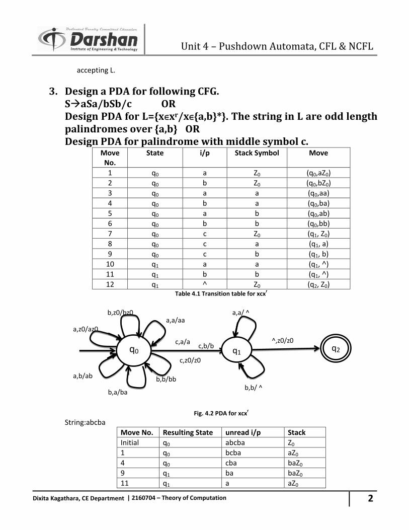
3. Design a PDA for following CFG. SaSa/bSb/c OR Design PDA for L={x∈xr/x∈{a,b}*}. The string in L are odd length palindromes over {a,b} OR Design PDA for palindrome with middle symbol c.
Move No.
State i/p Stack Symbol Move
1 q0 a Z0 (q0,aZ0)
2 q0 b Z0 (q0,bZ0)
3 q0 a a (q0,aa)
4 q0 b a (q0,ba)
5 q0 a b (q0,ab)
6 q0 b b (q0,bb)
7 q0 c Z0 (q1, Z0)
8 q0 c a (q1, a)
9 q0 c b (q1, b)
10 q1 a a (q1, ˄)
11 q1 b b (q1, ˄)
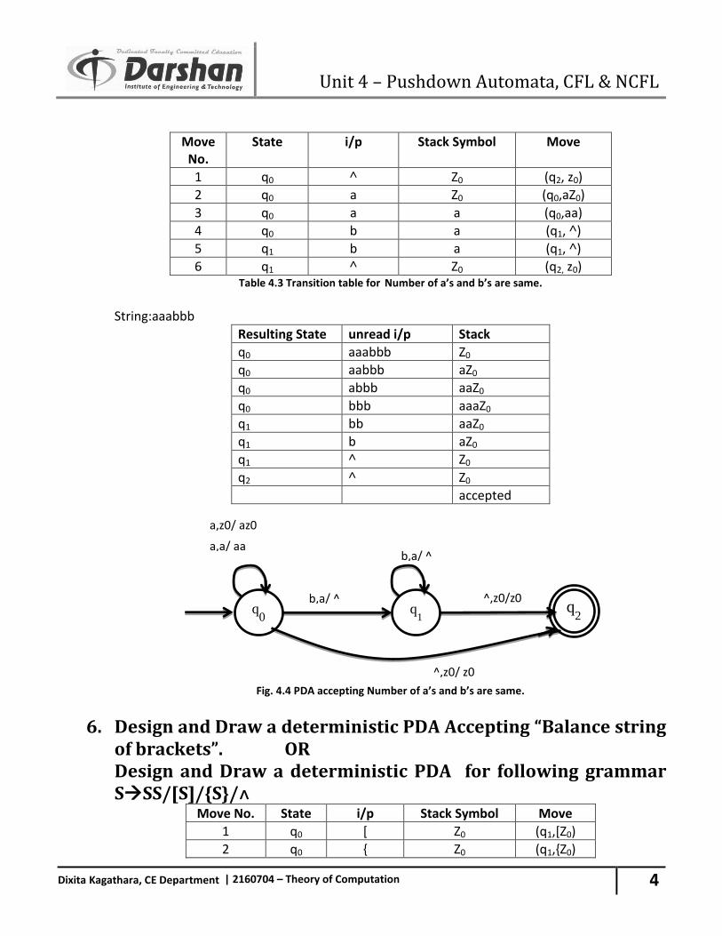
12 q1 ˄ Z0 (q2, Z0) Table 4.1 Transition table for xcx
r
Fig. 4.2 PDA for xcx
r String:abcba
Move No. Resulting State unread i/p Stack
Initial q0 abcba Z0
1 q0 bcba aZ0
4 q0 cba baZ0
9 q1 ba baZ0
11 q1 a aZ0
a,z0/az0
q0
b,z0/bz0 a,a/aa
a,b/ab
b,a/ba
b,b/bb
^,z0/z0
c,z0/z0
c,b/b
q1
a,a/ ^
q2
c,a/a
b,b/ ^
Unit 4 – Pushdown Automata, CFL & NCFL
3
Dixita Kagathara, CE Department | 2160704 – Theory of Computation
10 q1 ^ Z0
12 q2 ^ Z0
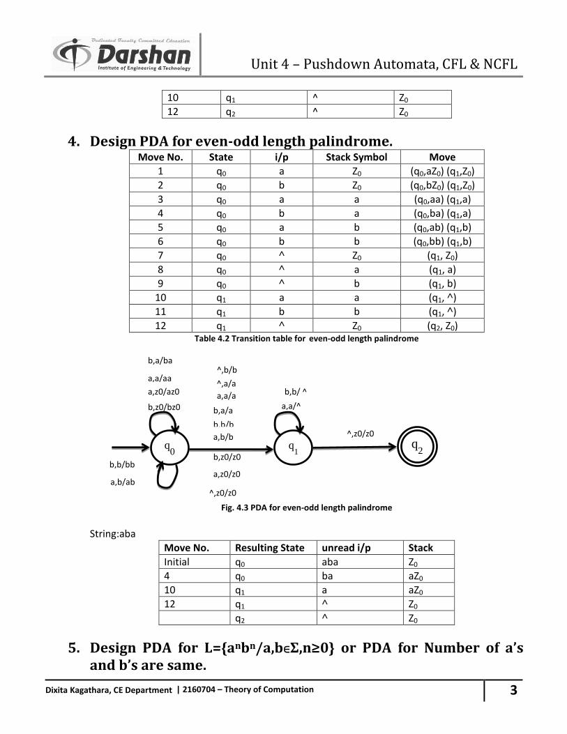
4. Design PDA for even-odd length palindrome. Move No. State i/p Stack Symbol Move
1 q0 a Z0 (q0,aZ0) (q1,Z0)
2 q0 b Z0 (q0,bZ0) (q1,Z0)
3 q0 a a (q0,aa) (q1,a)
4 q0 b a (q0,ba) (q1,a)
5 q0 a b (q0,ab) (q1,b)
6 q0 b b (q0,bb) (q1,b)
7 q0 ˄ Z0 (q1, Z0)
8 q0 ˄ a (q1, a)
9 q0 ˄ b (q1, b)
10 q1 a a (q1, ˄)
11 q1 b b (q1, ˄)
12 q1 ˄ Z0 (q2, Z0) Table 4.2 Transition table for even-odd length palindrome
Fig. 4.3 PDA for even-odd length palindrome
String:aba
Move No. Resulting State unread i/p Stack
Initial q0 aba Z0
4 q0 ba aZ0
10 q1 a aZ0
12 q1 ˄ Z0
q2 ˄ Z0
5. Design PDA for L={anbn/a,b∈Ʃ,n≥0} or PDA for Number of a’s and b’s are same.
a,z0/az0
q0
b,z0/bz0
q1
a,a/^
q2
b,z0/z0
a,z0/z0
^,z0/z0
b,b/b
a,b/ab
b,a/a
a,a/a
^,a/a
^,b/b
b,b/ ^
^,z0/z0 a,b/b
b,a/ba
a,a/aa
b,b/bb
Unit 4 – Pushdown Automata, CFL & NCFL
4
Dixita Kagathara, CE Department | 2160704 – Theory of Computation
Move
No. State i/p Stack Symbol Move
1 q0 ˄ Z0 (q2, z0)
2 q0 a Z0 (q0,aZ0)
3 q0 a a (q0,aa)
4 q0 b a (q1, ˄)
5 q1 b a (q1, ˄)
6 q1 ˄ Z0 (q2, z0) Table 4.3 Transition table for Number of a’s and b’s are same.
String:aaabbb
Resulting State unread i/p Stack
q0 aaabbb Z0
q0 aabbb aZ0
q0 abbb aaZ0
q0 bbb aaaZ0
q1 bb aaZ0
q1 b aZ0
q1 ˄ Z0
q2 ˄ Z0
accepted
Fig. 4.4 PDA accepting Number of a’s and b’s are same.
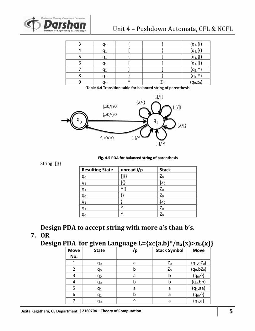
6. Design and Draw a deterministic PDA Accepting “Balance string of brackets”. OR Design and Draw a deterministic PDA for following grammar SSS/[S]/{S}/˄
Move No. State i/p Stack Symbol Move
1 q0 [ Z0 (q1,[Z0)
2 q0 { Z0 (q1,{Z0)
q0
q1
b,a/ ^
q2
^,z0/ z0
^,z0/z0
a,a/ aa
b,a/ ^
a,z0/ az0
Unit 4 – Pushdown Automata, CFL & NCFL
5
Dixita Kagathara, CE Department | 2160704 – Theory of Computation
3 q1 { { (q1,{{)
4 q1 [ { (q1,[{)
5 q1 { [ (q1,{[)
6 q1 [ [ (q1,[[)
7 q1 ] [ (q1,˄)
8 q1 } { (q1,˄)
9 q1 ˄ Z0 (q0,z0) Table 4.4 Transition table for balanced string of parenthesis
Fig. 4.5 PDA for balanced string of parenthesis
String: []{}
Resulting State unread i/p Stack
q0 []{} Z0
q1 ]{} [Z0
q1 ^{} Z0
q0 {} Z0
q1 } {Z0
q1 ˄ Z0
q0 ˄ Z0
7.
Design PDA to accept string with more a’s than b’s. OR Design PDA for given Language L={x∈{a,b}*/na(x)>nb(x)}
Move No.
State i/p Stack Symbol Move
1 q0 a Z0 (q1,aZ0)
2 q0 b Z0 (q0,bZ0)
3 q0 a b (q0,˄)
4 q0 b b (q0,bb)
5 q1 a a (q1,aa)
6 q1 b a (q0,˄)
7 q0 ˄ a (q1,a)
q0
{,{/{{
q1
{,[/{[
[,{/[{
[,[/[[
^,z0/z0 },{/ ^
],[/˄
{,z0/{z0
[,z0/[z0
Unit 4 – Pushdown Automata, CFL & NCFL
6
Dixita Kagathara, CE Department | 2160704 – Theory of Computation
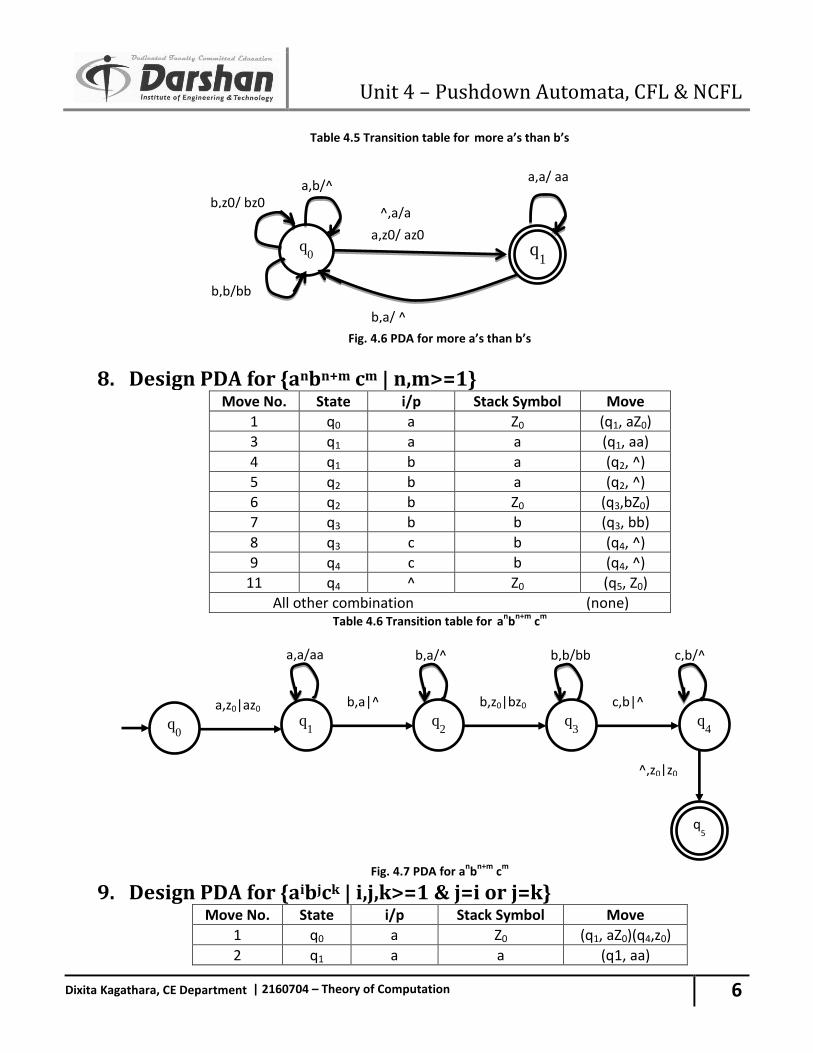
Table 4.5 Transition table for more a’s than b’s
Fig. 4.6 PDA for more a’s than b’s
8. Design PDA for {anbn+m cm | n,m>=1} Move No. State i/p Stack Symbol Move
1 q0 a Z0 (q1, aZ0)
3 q1 a a (q1, aa)
4 q1 b a (q2, ^)
5 q2 b a (q2, ^)
6 q2 b Z0 (q3,bZ0)
7 q3 b b (q3, bb)
8 q3 c b (q4, ^)
9 q4 c b (q4, ^)
11 q4 ^ Z0 (q5, Z0)
All other combination (none) Table 4.6 Transition table for an
bn+m
cm
Fig. 4.7 PDA for anb
n+m c
m
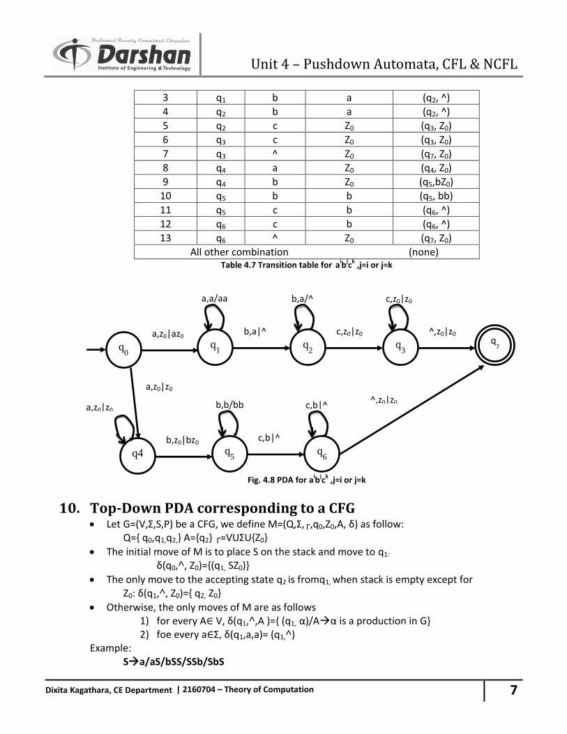
9. Design PDA for {aibjck | i,j,k>=1 & j=i or j=k} Move No. State i/p Stack Symbol Move
1 q0 a Z0 (q1, aZ0)(q4,z0)
2 q1 a a (q1, aa)
q1
a,b/^ b,z0/ bz0
q0
b,b/bb
a,a/ aa
b,a/ ^
a,z0/ az0
^,a/a
q0
a,z0|az0 q
1
b,a|^
q2
b,z0|bz0
q3
c,b|^
q4
^,z0|z0
a,a/aa b,a/^ b,b/bb c,b/^
q5
Unit 4 – Pushdown Automata, CFL & NCFL
7
Dixita Kagathara, CE Department | 2160704 – Theory of Computation
3 q1 b a (q2, ^)
4 q2 b a (q2, ^)
5 q2 c Z0 (q3, Z0)
6 q3 c Z0 (q3, Z0)
7 q3 ^ Z0 (q7, Z0)
8 q4 a Z0 (q4, Z0)
9 q4 b Z0 (q5,bZ0)
10 q5 b b (q5, bb)
11 q5 c b (q6, ^)
12 q6 c b (q6, ^)
13 q6 ^ Z0 (q7, Z0)
All other combination (none) Table 4.7 Transition table for ai
bjc
k ,j=i or j=k
Fig. 4.8 PDA for aib
jc
k ,j=i or j=k
10. Top-Down PDA corresponding to a CFG Let G=(V,Ʃ,S,P) be a CFG, we define M=(Q,Ʃ,┌,q0,Z0,A, δ) as follow:
Q={ q0,q1,q2,} A={q2} ┌=VUƩU{Z0}
The initial move of M is to place S on the stack and move to q1:
δ(q0,˄, Z0)={(q1, SZ0)}
The only move to the accepting state q2 is fromq1, when stack is empty except for Z0: δ(q1,˄, Z0)={ q2, Z0}
Otherwise, the only moves of M are as follows 1) for every A∈ V, δ(q1,˄,A )={ (q1, α)/Aα is a production in G} 2) foe every a∈Ʃ, δ(q1,a,a)= (q1,˄)
Example: Sa/aS/bSS/SSb/SbS
q7
^,z0|z0
a,a/aa b,a/^ c,z0|z0
q0
a,z0|az0 q
1
b,a|^
q2
c,z0|z0
q3
^,z0|z0
b,b/bb c,b|^
q4
b,z0|bz0 q
5
c,b|^
a,z0|z0
a,z0|z0
q6
Unit 4 – Pushdown Automata, CFL & NCFL
8
Dixita Kagathara, CE Department | 2160704 – Theory of Computation
Move No. State i/p Stack Symbol Move
1 q0 ˄ Z0 (q1,SZ0)
2 q1 ˄ S (q1,a) (q1,aS) (q1,bSS) (q1,SSb) (q1,SbS)
3 q1 a a (q1,˄)
4 q1 b b (q1,˄)
5 q1 ˄ Z0 (q2, Z0) Table 4.8 Top down PDA equivalent to CFG
(q0,abbaaa, Z0) ⊢(q1,abbaaa, SZ0) ⊢(q1,abbaaa, SbSZ0) ⊢(q1,abbaaa, abSZ0) ⊢(q1,bbaaa, bSZ0) ⊢(q1,baaa, SZ0) ⊢(q1,baaa, bSSZ0) ⊢(q1,aaa, SSZ0) ⊢(q1,aaa, aSZ0) ⊢(q1, aa,SZ0) ⊢(q1,aa, aSZ0) ⊢(q1, a, SZ0) ⊢(q1, a, aZ0) ⊢(q1,˄, Z0) ⊢(q2,˄, Z0)
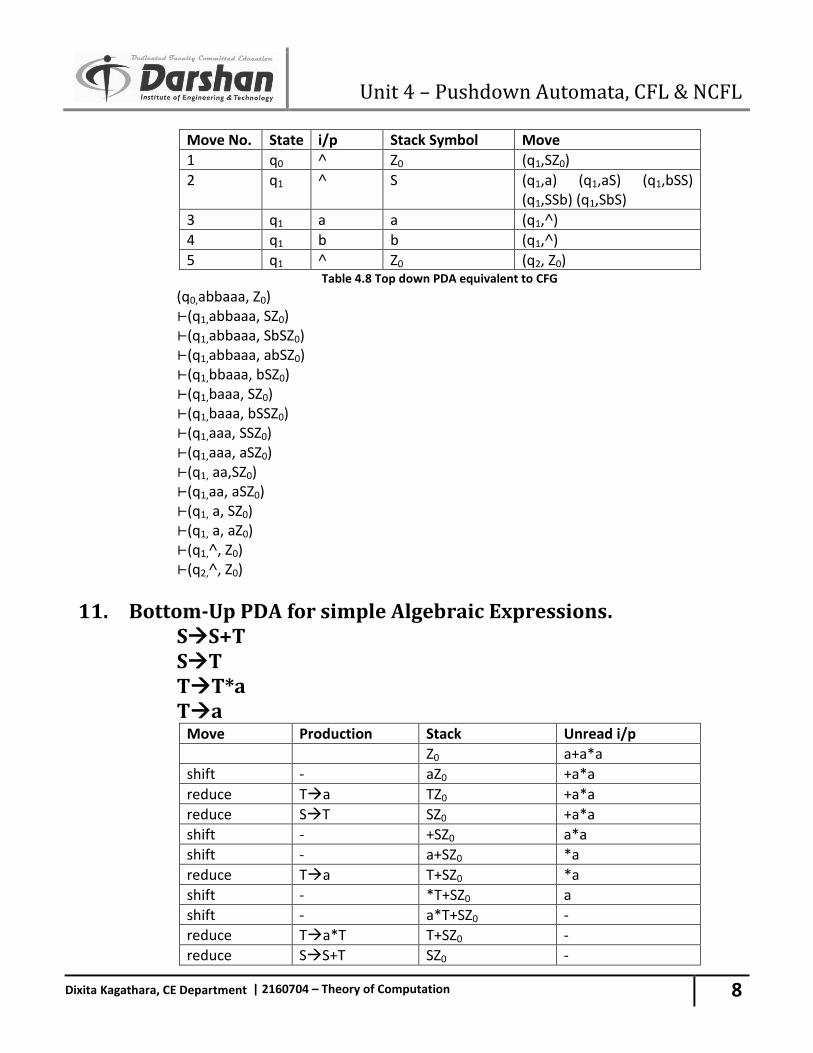
11. Bottom-Up PDA for simple Algebraic Expressions. SS+T
ST TT*a Ta
Move Production Stack Unread i/p
Z0 a+a*a
shift - aZ0 +a*a
reduce Ta TZ0 +a*a
reduce ST SZ0 +a*a
shift - +SZ0 a*a
shift - a+SZ0 *a
reduce Ta T+SZ0 *a
shift - *T+SZ0 a
shift - a*T+SZ0 -
reduce Ta*T T+SZ0 -
reduce SS+T SZ0 -
Unit 4 – Pushdown Automata, CFL & NCFL
9
Dixita Kagathara, CE Department | 2160704 – Theory of Computation
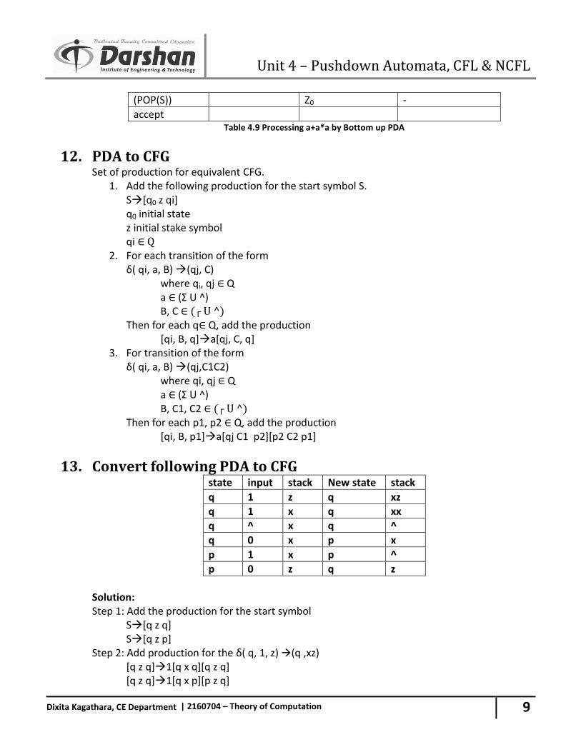
(POP(S)) Z0 -
accept Table 4.9 Processing a+a*a by Bottom up PDA
12. PDA to CFG Set of production for equivalent CFG.
1. Add the following production for the start symbol S. S[q0 z qi]
q0 initial state z initial stake symbol qi ∈ Q
2. For each transition of the form δ( qi, a, B) (qj, C) where qi, qj ∈ Q a ∈ (Ʃ U ^) B, C ∈ (┌ U ^) Then for each q∈ Q, add the production [qi, B, q]a[qj, C, q]
3. For transition of the form δ( qi, a, B) (qj,C1C2) where qi, qj ∈ Q a ∈ (Ʃ U ^) B, C1, C2 ∈ (┌ U ^) Then for each p1, p2 ∈ Q, add the production [qi, B, p1]a[qj C1 p2][p2 C2 p1]
13. Convert following PDA to CFG state input stack New state stack
q 1 z q xz
q 1 x q xx
q ^ x q ^
q 0 x p x
p 1 x p ^
p 0 z q z
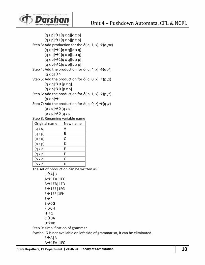
Solution: Step 1: Add the production for the start symbol S[q z q] S[q z p] Step 2: Add production for the δ( q, 1, z) (q ,xz) [q z q]1[q x q][q z q] [q z q]1[q x p][p z q]
Unit 4 – Pushdown Automata, CFL & NCFL
10
Dixita Kagathara, CE Department | 2160704 – Theory of Computation
[q z p]1[q x q][q z p] [q z p]1[q x p][p z p] Step 3: Add production for the δ( q, 1, x) (q ,xx) [q x q]1[q x q][q x q] [q x q]1[q x p][p x q] [q x p]1[q x q][q x p] [q x p]1[q x p][p x p] Step 4: Add the production for δ( q, ^, x) (q ,^) [q x q]^ Step 5: Add the production for δ( q, 0, x) (p ,x) [q x q]0 [p x q] [q x p]0 [p x p] Step 6: Add the production for δ( p, 1, x) (p ,^) [p x p]1 Step 7: Add the production for δ( p, 0, z) (q ,z) [p z q]0 [q z q] [p z p]0 [q z p] Step 8: Renaming variable name
Original name New name
[q z q] A
[q z p] B
[p z q] C
[p z p] D
[q x q] E
[q x p] F
[p x q] G
[p x p] H
The set of production can be written as: SA|B A1EA|1FC B1EB|1FD E1EE|1FG F1EF|1FH E^ E0G F0H H1 C0A D0B Step 9: simplification of grammar Symbol G is not available on left side of grammar so, it can be eliminated. SA|B A1EA|1FC
Unit 4 – Pushdown Automata, CFL & NCFL
11
Dixita Kagathara, CE Department | 2160704 – Theory of Computation
B1EB|1FD E1EE|^ F1EF|1FH|0H H1 C0A D0B
14. Intersection and complement of CFL (Non CFL) Theorem:-There are CFLs L1 and L2 so that L1∩ L2 is not a CFL, and there is a CFL L so that L’ is
not a CFL. we observed that L= { aibjck| i < j and i < k } is not context-free. However, although no PDA can test both conditions i < j and i< k simultaneously, it is easy enough to build two PDAs that test the conditions separately. In other words, although the intersection L of the two languages L1 = {a i bjck | i < j} and L2 = {aibjck | i < k} is not a CFL, both languages themselves are. Another way to verify that L1 is a CFL is to check it is generated by the grammar with productions SABC AaAb|˄ BbB|b CcC|˄ Similarly, L2is generated by the CFG with productions SAC AaAc|B BbB|˄ CcC|c The second statement in the theorem follows from the first and the formula L1∩ L2 =( L1’U L2’)’ If complements of CFLs were always CFLs, then for any CFLs L1 and L2, the language L1’and L2’ would be CFLs, so would their union, and so would its complement. We know now that this is not the case.
15. Give the difference between Top Down & Bottom Up parsing. Top Down Parsing Bottom Up Parsing
A parser is top-down if it discovers a parse tree top to bottom
A top down parser for a given grammar G tries to derive a string through a sequence of derivation starting with a start symbol.
Top down parsing methods are: Top down parsing(with
backtracking/without backtracking)
Recursive decent parser
A parser is bottom up if it discovers a parse tree bottom to top
In bottom up parsing, the source string is reduced to the start symbol of the grammar. Bottom up parsing method is also called shift reduce parsing.
Bottom up parsing methods are: Naïve bottom up parsing Operator precedence
parsing
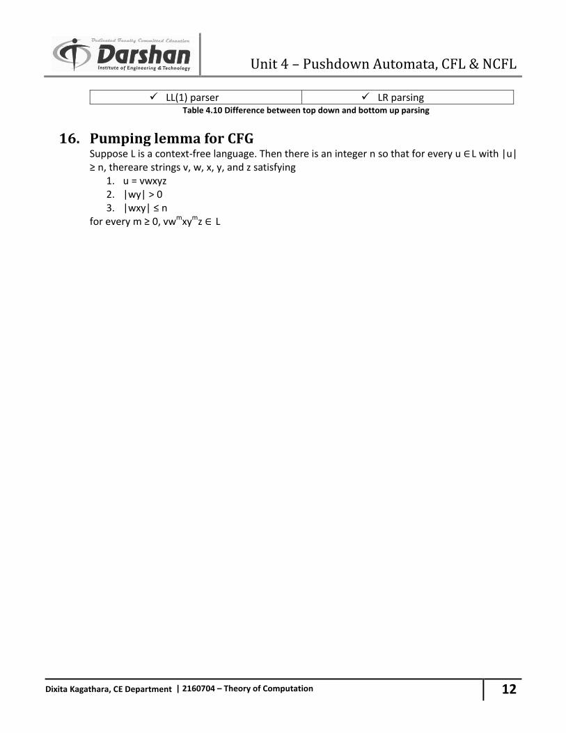
Unit 4 – Pushdown Automata, CFL & NCFL
12
Dixita Kagathara, CE Department | 2160704 – Theory of Computation
LL(1) parser LR parsing Table 4.10 Difference between top down and bottom up parsing
16. Pumping lemma for CFG Suppose L is a context-free language. Then there is an integer n so that for every u ∈ L with |u|
≥ n, thereare strings v, w, x, y, and z satisfying 1. u = vwxyz 2. |wy| > 0 3. |wxy| ≤ n
for every m ≥ 0, vwmxymz ∈ L
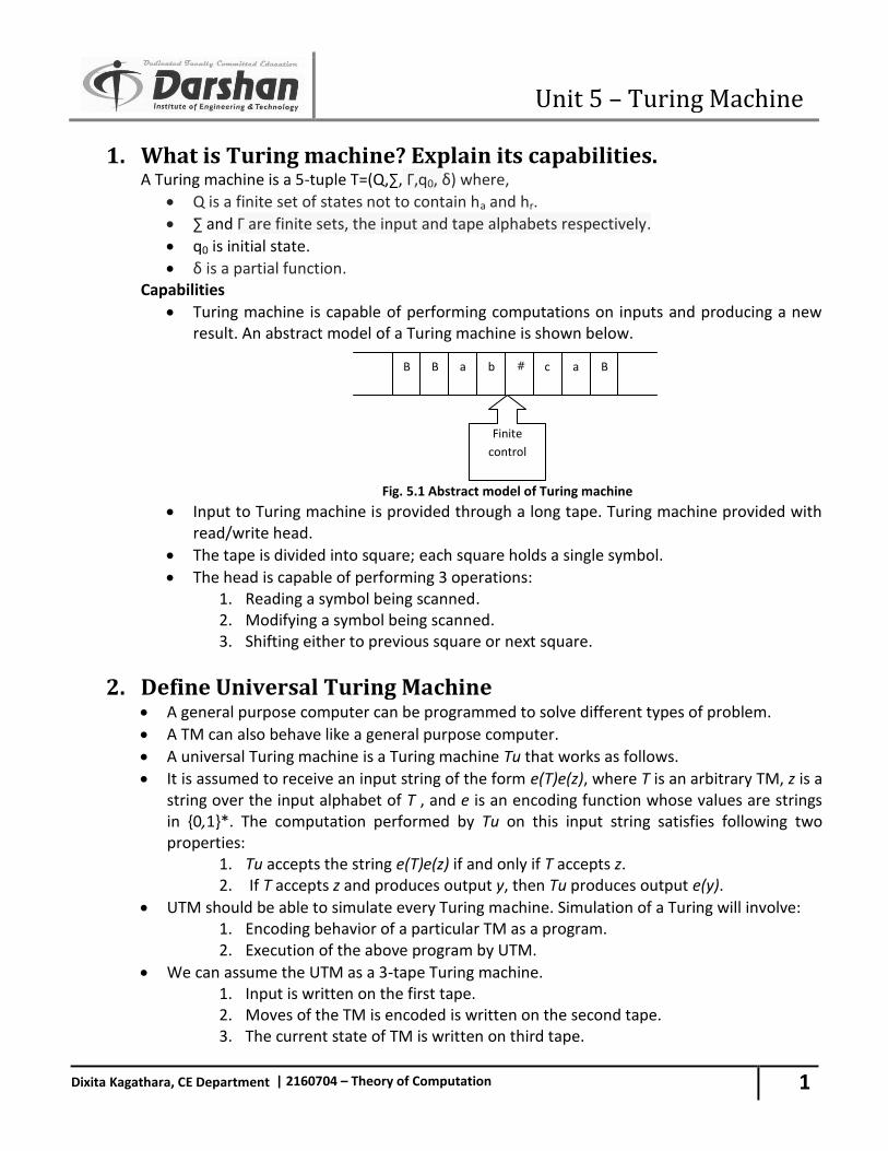
Unit 5 – Turing Machine
1
Dixita Kagathara, CE Department | 2160704 – Theory of Computation
1. What is Turing machine? Explain its capabilities. A Turing machine is a 5-tuple T=(Q,∑, Γ,q0, δ) where,
Q is a finite set of states not to contain ha and hr.
∑ and Γ are finite sets, the input and tape alphabets respectively.
q0 is initial state.
δ is a partial function. Capabilities
Turing machine is capable of performing computations on inputs and producing a new result. An abstract model of a Turing machine is shown below.
Fig. 5.1 Abstract model of Turing machine
Input to Turing machine is provided through a long tape. Turing machine provided with read/write head.
The tape is divided into square; each square holds a single symbol.
The head is capable of performing 3 operations: 1. Reading a symbol being scanned. 2. Modifying a symbol being scanned. 3. Shifting either to previous square or next square.
2. Define Universal Turing Machine A general purpose computer can be programmed to solve different types of problem.
A TM can also behave like a general purpose computer.
A universal Turing machine is a Turing machine Tu that works as follows.
It is assumed to receive an input string of the form e(T)e(z), where T is an arbitrary TM, z is a string over the input alphabet of T , and e is an encoding function whose values are strings in {0,1}*. The computation performed by Tu on this input string satisfies following two properties:
1. Tu accepts the string e(T)e(z) if and only if T accepts z. 2. If T accepts z and produces output y, then Tu produces output e(y).
UTM should be able to simulate every Turing machine. Simulation of a Turing will involve: 1. Encoding behavior of a particular TM as a program. 2. Execution of the above program by UTM.
We can assume the UTM as a 3-tape Turing machine. 1. Input is written on the first tape. 2. Moves of the TM is encoded is written on the second tape. 3. The current state of TM is written on third tape.
B B a b # c a B
Finite
control
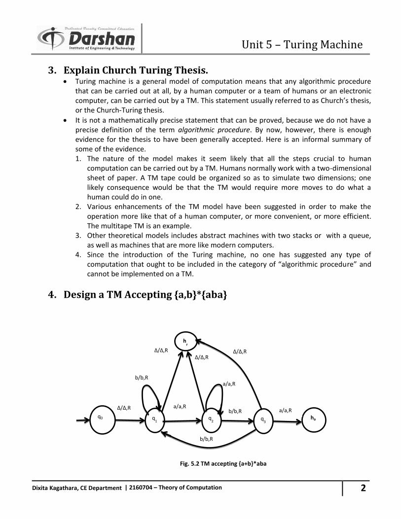
Unit 5 – Turing Machine
2
Dixita Kagathara, CE Department | 2160704 – Theory of Computation
3. Explain Church Turing Thesis. Turing machine is a general model of computation means that any algorithmic procedure
that can be carried out at all, by a human computer or a team of humans or an electronic computer, can be carried out by a TM. This statement usually referred to as Church’s thesis, or the Church-Turing thesis.
It is not a mathematically precise statement that can be proved, because we do not have a precise definition of the term algorithmic procedure. By now, however, there is enough evidence for the thesis to have been generally accepted. Here is an informal summary of some of the evidence. 1. The nature of the model makes it seem likely that all the steps crucial to human
computation can be carried out by a TM. Humans normally work with a two-dimensional sheet of paper. A TM tape could be organized so as to simulate two dimensions; one likely consequence would be that the TM would require more moves to do what a human could do in one.
2. Various enhancements of the TM model have been suggested in order to make the operation more like that of a human computer, or more convenient, or more efficient. The multitape TM is an example.
3. Other theoretical models includes abstract machines with two stacks or with a queue, as well as machines that are more like modern computers.
4. Since the introduction of the Turing machine, no one has suggested any type of computation that ought to be included in the category of “algorithmic procedure” and cannot be implemented on a TM.
4. Design a TM Accepting {a,b}*{aba}
Fig. 5.2 TM accepting {a+b}*aba
b/b,R
∆/∆,R
∆/∆,R
q0 q1
Q
1
q2
b/b,R
∆/∆,R
q3
ha
hr
a/a,R
a/a,R b/b,R
∆/∆,R
a/a,R
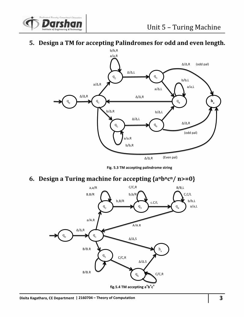
Unit 5 – Turing Machine
3
Dixita Kagathara, CE Department | 2160704 – Theory of Computation
5. Design a TM for accepting Palindromes for odd and even length.
Fig. 5.3 TM accepting palindrome string
6. Design a Turing machine for accepting {anbncn/ n>=0}
fig.5.4 TM accepting a
nb
nc
n
∆/∆,R
c,C/L
q0
b,B/R
q1
b/b,L
q2 q
3 q
4
q6
a/A,R
ha B/B,R
A/A,R
q5
∆/∆,S
C,C/L B,B/R
C/C,R
a,a/R B/B,L
∆/∆,S
B/B,R
b,b/R
C/C,R
C/C,R
a/a,L
a/∆,R
∆/∆,L
∆/∆,R
q0 q
1
q2
q5
a/a,R
∆/∆,R q6
q3
a/a,R
q4
(Even pal)
ha
b/∆,R
∆/∆,R
b/b,L
b/∆,L
(odd pal)
a/∆,L
∆/∆,R
∆/∆,L
a/a,L
b/b,R
∆/∆,R
b/b,R
(odd pal)
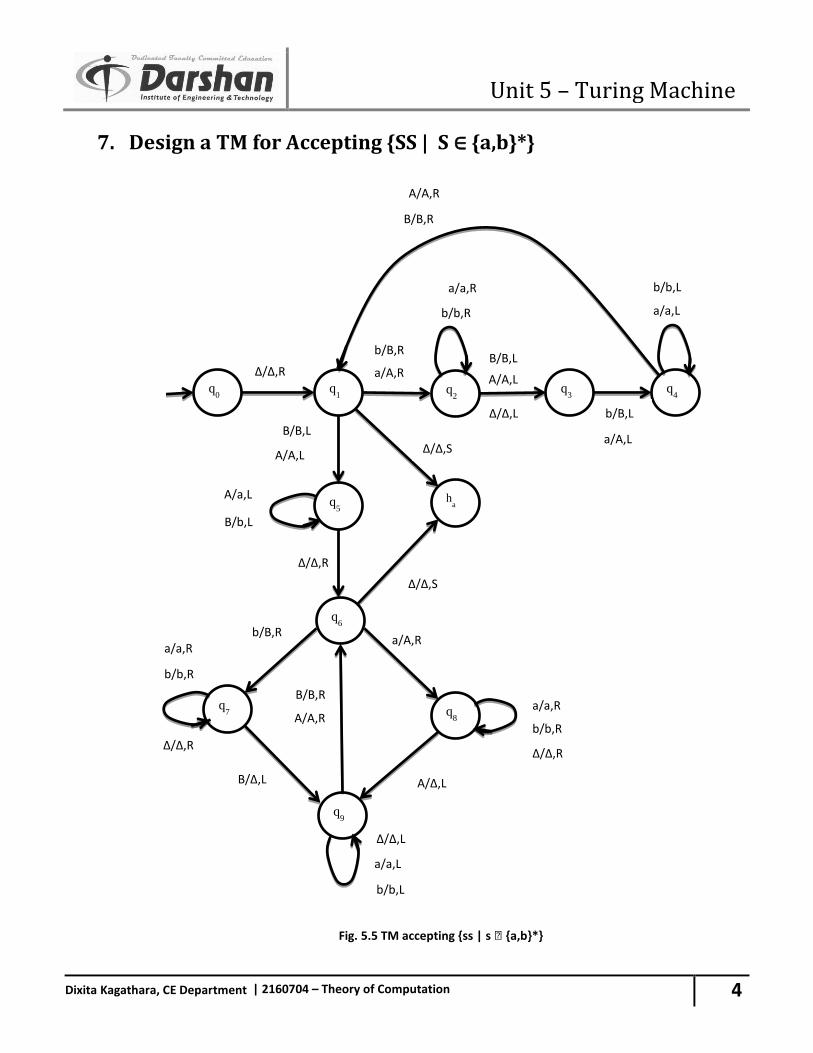
Unit 5 – Turing Machine
4
Dixita Kagathara, CE Department | 2160704 – Theory of Computation
7. Design a TM for Accepting {SS | S ∈ {a,b}*}
Fig. 5.5 TM accepting {ss | s ∈ {a,b}*}
B/B,L
A/A,L
∆/∆,R
q0 q
1
∆/∆,L
q2 q
3 q
4
q5 h
a
q6
q7
q9
B/B,R
q8
A/a,L
a/A,R
∆/∆,S
B/B,R
B/b,L
∆/∆,L
∆/∆,S
A/A,R
∆/∆,R
∆/∆,R ∆/∆,R
a/A,R
b/B,R
b/b,R
a/a,R
A/A,R
B/B,L
b/B,L
a/A,L
a/a,L
b/b,L
A/A,L
a/a,R
b/b,R
b/B,R
B/∆,L A/∆,L
a/a,L
b/b,L
a/a,R
b/b,R
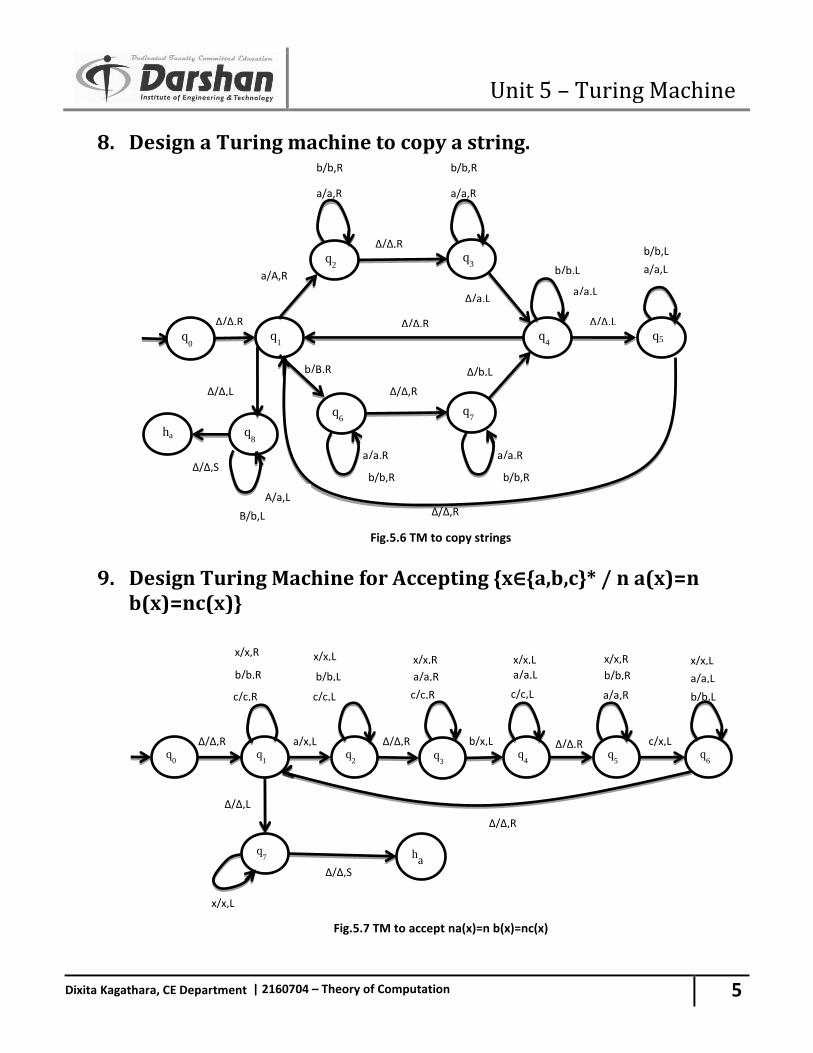
Unit 5 – Turing Machine
5
Dixita Kagathara, CE Department | 2160704 – Theory of Computation
8. Design a Turing machine to copy a string.
Fig.5.6 TM to copy strings
9. Design Turing Machine for Accepting {x∈{a,b,c}* / n a(x)=n b(x)=nc(x)}
Fig.5.7 TM to accept na(x)=n b(x)=nc(x)
c/x,L a/x,L ∆/∆,R ∆/∆,R
R q0 q
1
∆/∆,R
q7 h
a
b/x,L q
2 q
3 q
4 q
5 q
6
∆/∆,L
c/c,R b/b,L c/c,R c/c,L c/c,L a/a,R
x/x,L
∆/∆,S
∆/∆,R
b/b,R b/b,L a/a,R a/a,L b/b,R a/a,L
x/x,R x/x,L x/x,R x/x,L x/x,R x/x,L
a/A,R
∆/∆,R
∆/∆,R
q8
q1
q2
q6
a/a,R
∆/∆,L
q7
q3
a/a,R
q4 q5
b/B,R
∆/∆,R
b/b,L
∆/b,L
∆/a,L
∆/∆,R
∆/∆,R
a/a,L
b/b,R
∆/∆,L
b/b,R
a/a,R
b/b,R
a/a,R
b/b,R
q0
ha
∆/∆,S
A/a,L
B/b,L
a/a,L
b/b,L
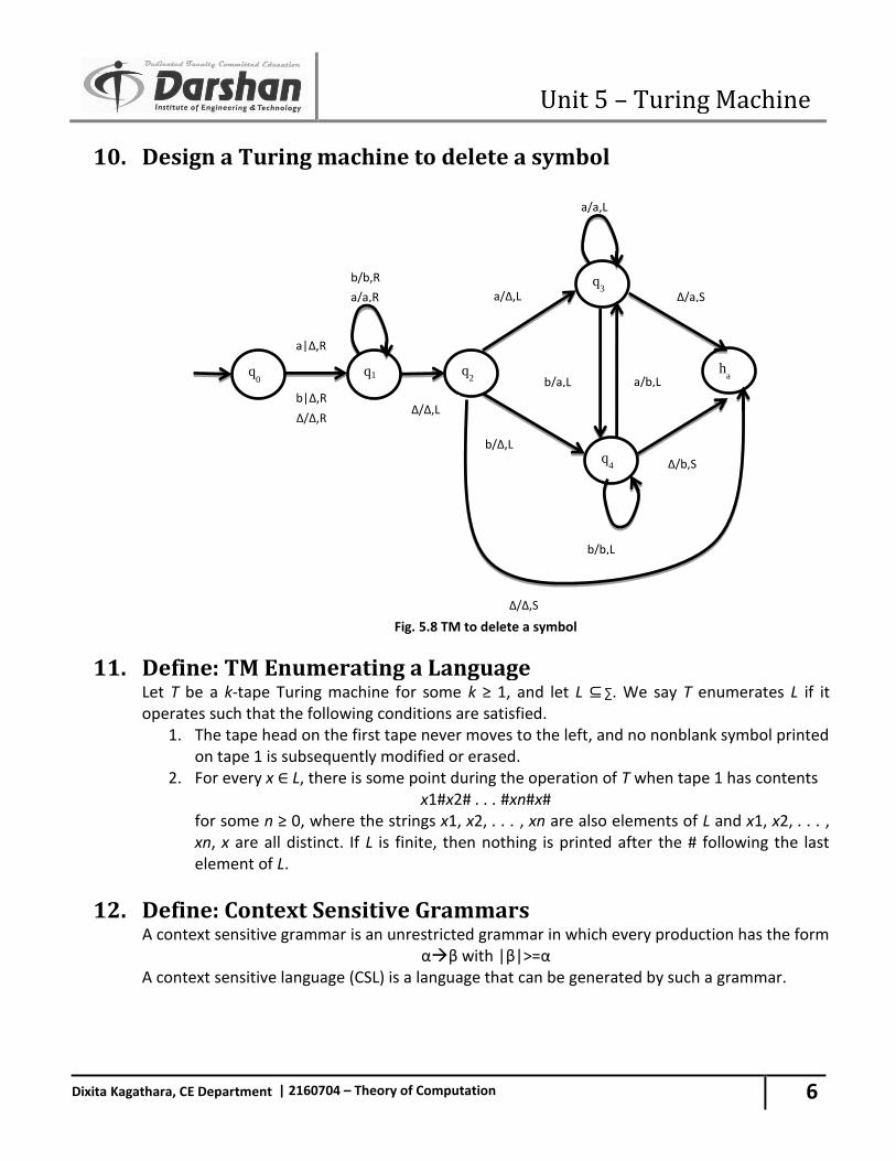
Unit 5 – Turing Machine
6
Dixita Kagathara, CE Department | 2160704 – Theory of Computation
10. Design a Turing machine to delete a symbol
Fig. 5.8 TM to delete a symbol
11. Define: TM Enumerating a Language Let T be a k-tape Turing machine for some k ≥ 1, and let L ⊆ ∑. We say T enumerates L if it
operates such that the following conditions are satisfied. 1. The tape head on the first tape never moves to the left, and no nonblank symbol printed
on tape 1 is subsequently modified or erased. 2. For every x ∈ L, there is some point during the operation of T when tape 1 has contents
x1#x2# . . . #xn#x# for some n ≥ 0, where the strings x1, x2, . . . , xn are also elements of L and x1, x2, . . . , xn, x are all distinct. If L is finite, then nothing is printed after the # following the last element of L.
12. Define: Context Sensitive Grammars A context sensitive grammar is an unrestricted grammar in which every production has the form
αβ with |β|>=α A context sensitive language (CSL) is a language that can be generated by such a grammar.
∆/∆,S
ha
q3
∆/a,S
∆/b,S q4
a/a,L
b/b,L
b/a,L a/b,L q
2
∆/∆,L
a/∆,L
b/∆,L
∆/∆,R
q1 q0
a/a,R
b/b,R
a|∆,R
b|∆,R
Unit 6 – Computable Functions
1
Dixita Kagathara, CE Department | 2160704 – Theory of Computation
1. Define the following terms: Initial Function
The initial function are the following: 1. Constant functions: For each k ≥ 0 and each a ≥ 0, the constant function
: Nk→ N is defined by the formula
(X) = a for every X Nk
In the case k = 0 we may identify the function with the number a.
2. The successor function s : N → N is defined by the formula s(x) = x + 1
3. Projection functions: For each k ≥ 1 and each i with 1 ≤ i ≤ k, the projection function
:Nk→ N is defined by the formula
(x1, x2, … , xi, …., xk) = xi
Composition Suppose f is a partial function from Nk to N, and for each i with 1 ≤ i ≤ k, gi is a partial function from Nm to N. The partial function obtained from f and g1, g2, ... , gk by composition is the partial function h from Nm to N defined by the formula
h(X) = f(g1(X), g2(X), .. , gk(X)) (X ε Nm) Primitive Recursion Operation Suppose n ≥ 0, and g and h are functions of n and n + 2 variables, respectively. The function obtained from g and h by the operation of primitive recursion is the function f : Nn+1→ N defined by the formulas
f(X,0) = g(X) f(X, k + 1) = h(X, k, f(x, k)) for every X Nn and every k ≥ 0.
Primitive Recursive Functions The set PR of primitive recursive functions is defined as follows.
1. All initial functions are elements of PR. 2. For any k ≥ 0 and m ≥ 0, if f : Nk→ N and g1, g2, ... , gk : N
m→ N are elements of PR, then the function f(g1, g2, ... , gk) obtained from f and g1, g2, ... , gk by composition is an element of PR.
3. For any n ≥ 0, any function g : Nn+1→ N in PR, and any function h : Nn+2→ N in PR, the function f : Nn + 1→ N obtained from g and h by primitive recursion is in PR.
4. No other functions are in the set PR. Bounded Quantifications Let P be an (n + 1)-place predicate. The bounded existential quantification of P is the (n + 1)-place predicate Ep defined by
Ep(X, k) = (there exists y with 0 ≤ y ≤ k such that P(X, y) is true) The bounded universal quantification of P is the (n + 1)-place predicate AP defined by
AP(X, k) = (for every y satisfying 0 ≤ y ≤ k, P(X, y) is true) Unbounded Minimalization If P is an (n + 1)-place predicate, the unbounded minimalization of P is the partial function MP : Nn→ N defined by
Mp(X) = min {y | P(X, y) is true}
Unit 6 – Computable Functions
2
Dixita Kagathara, CE Department | 2160704 – Theory of Computation
Mp(X) is undefined at any X ε Nn for which there is no y satisfying P(X, y). The notation μy[P(X, y)] is also used for Mp(X). In the special case in which P(X, y) = (f(X, y) = 0), we write Mp = Mf and refer to this function as the unbounded minimalization of f. Bounded Minimalization For an (n + 1)-place predicate P, the bounded minimalization of P is the function mp : Nn+1→ N defined by min {y | 0 ≤ y ≤ k and P(X, y)} if this set is not empty mp(X, k) = k + 1 otherwise The symbol μ is often used for the minimalization operator, and we sometimes write
mP(X, k) = y[P(X, y)] An important special case is that in which P(X, y) is (f(X, y) = 0), for some f :Nn+ 1→ N. In this case mp is written mf and referred to as the bounded minimalization of f. μ – Recursive Functions The set M of μ - recursive, or simply recursive, partial functions is defined as follows.
1. Every initial function is an element of M. 2. Every function obtained from elements of M by composition or primitive recursion is an
element of M. 3. For every n ≥ 0 and every total function f : Nn+1→ N in M, the function Mf : N
n→ N defined by
Mf(X) = μy[f(X, y) = 0] is an element of M. 4. No other functions are in the set M.
Gödel Number of a sequence of Natural Numbers For any finite sequence x0, x1, … , xn of natural numbers, the Gödel Number of the sequence is the number
gn(x0, x1, … , xn) = 2x03x15x2 … (PrNo(n))xn Where PrNo(n) is the nth prime.
2. Theorem: Let f: Ʃ1*Ʃ2*. Then f is computable if and only if f is μ-recursive.
Proof:
As above, we denote by g1 and g2 the Godel-numbering function for the two alphabets, and by g1’ and g2’ their respective left inverse.
Suppose on the hand that f is computable, and let Tf be a TM (whose tape alphabet contains the symbols of Ʃ1 and Ʃ2) computing f.
We want to show that pf :NN is μ-recursive, it is sufficient to show that pf that a composite Turing machine can be constructed form three simpler ones: one that takes the initial tape ∆1n and halts with tape ∆ g1’; the TM Tf, which then halts with tape ∆f(g1’(n)); and a third that calculates the Godel number of this string to yield the result, g2 (f(g1’(n)))= ρf(n).
On the other hand, suppose that f is μ-recursive. Then by definition, pf is μ-recursive. Let T be a TM computing it. From the formula for pf we have
g2’(ρf(n))= g2’(g2(f(g1’(n)))) = f(g1’(n))
Unit 6 – Computable Functions
3
Dixita Kagathara, CE Department | 2160704 – Theory of Computation
for any n. applying this formula when n= g1(x), we obtain f(x)=f(g1’(g1(x)))= g2’(ρf(g1(x)))
Just as before, we can now construct a composite TM Tf to perform this computation, and it follows that f is computable.


![arXiv:1505.04890v1 [cs.IT] 19 May 2015 · PDF fileA Natural Data Storage: A Review on sending Information from now to then via Nature Dixita Limbachiya, Dhirubhai Ambani Institute](https://img.pdfslide.us/doc/110x75/5a93f25a7f8b9a451b8bcd3d/arxiv150504890v1-csit-19-may-2015-natural-data-storage-a-review-on-sending.jpg)