Embed Size (px)
Citation preview
Overview of graphics system and output primitives (By Bishnu Rawal) Page 1
Unit 1 Overview of graphics systems and output primitives
Computer Graphics Computer Graphics is a field related to creation, storage, and manipulation of images of objects using computers. These objects come from diverse fields such as physical, mathematical, engineering, architectural, abstract structures and natural phenomenon.
In reality, Computer graphics refer different things in different contexts: – Pictures, scenes that are generated by a computer. – Tools used to make such pictures, software and hardware, input/output devices. – The whole field of study that involves these tools and the pictures they produce.
Trends on Computer Graphics
Until the early 1980's computer graphics was a small, specialized field, largely because the hardware was expensive and graphics-based application programs that were easy to use and cost-effective were few. Then, personal computers with built-in raster graphics displays-such as the Xerox Star, Apple Macintosh and the IBM PC- popularized the use of bitmap graphics for user-computer interaction. A bitmap is an ones and zeros representation of the rectangular array points on the screen. Each point is called a pixel, short for "Picture Elements”. Once bitmap graphics became affordable, and explosion of easy-to-use and inexpensive graphics-based applications soon followed. Graphics-based user interfaces allowed millions of new users to control simple, low-cost application programs, such as word-processors, spreadsheets, and drawing programs.
Today, almost all interactive application programs, even those for manipulating text (e.g. word processor) or numerical data (e.g. spreadsheet programs), use graphics extensively in the user interface and for visualizing and manipulating the application-specific objects. Even people who do not use computers encounter computer graphics in TV commercials and as cinematic special effects. Computer graphics is no longer a rarity. It is an integral part of all computer user interfaces, and is indispensable for visualizing 2D, 3D objects in diverse areas such as education, science, engineering, medicine, commerce, the military, advertising, and entertainment.
Historical background Guys, Its quite descriptive but interesting one being pictorial, read/see thoroughly. Some sections provide important video URLs, please see them if feasible.
Prehistory The foundations of computer graphics can be traced to artistic and mathematical ``inventions,'' for example,
Euclid (circa 300 - 250 BC) who's formulation of geometry provides a basis for graphics concepts. Filippo Brunelleschi (1377 - 1446) architect, goldsmith, and sculptor who is noted for his use of
perspective. Rene Descartes’ (1596-1650) who developed analytic geometry, in particular coordinate systems
which provide a foundation for describing the location and shape of objects in space. Gottfried Wilhelm Leibniz (1646 - 1716) and Isaac Newton (1642 - 1727) who co-invented
calculus that allow us to describe dynamical systems. James Joseph Sylvester (1814 - 1897) who invented matrix notation. A lot of graphics can be
done with matrices.
www.csitportal.com
Overview of graphics system and output primitives (By Bishnu Rawal) Page 2
I. Schoenberg who discovered splines, a fundamental type of curve.
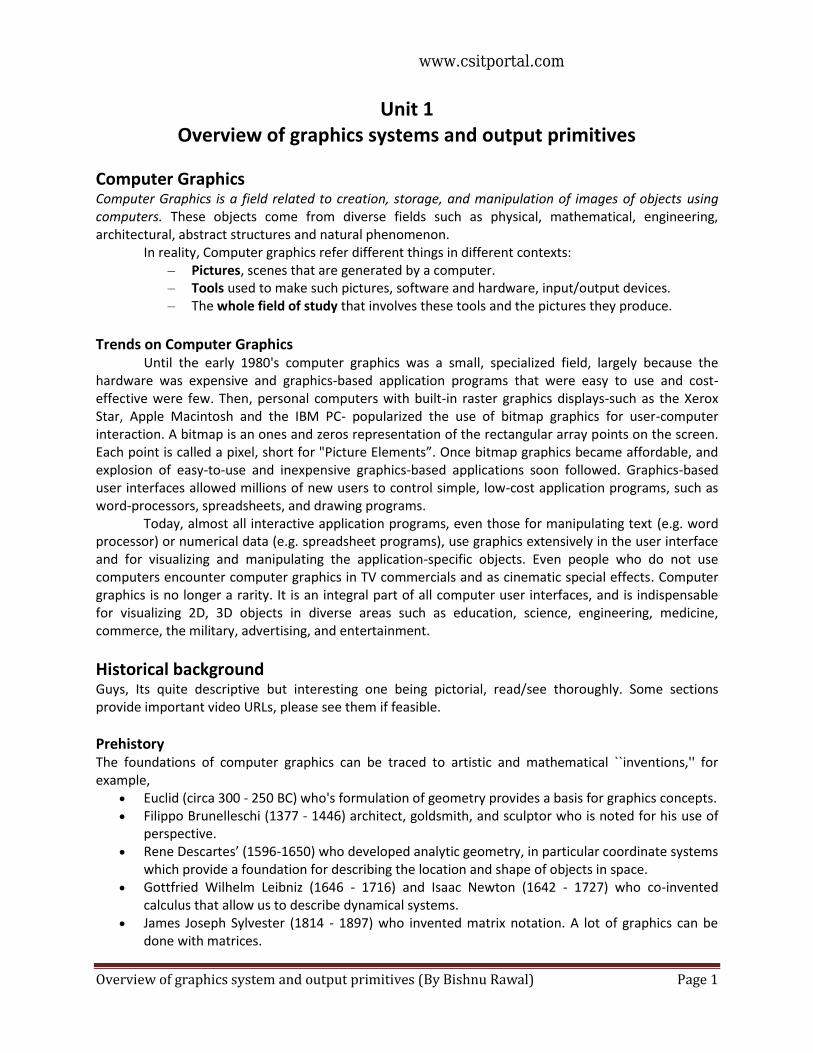
1941
Although the punched card was first used in 1801 to control textile looms, they were first used as an input medium for “computing machines” in 1941. Special typewriter-like devices were used to punch holes through sheets of think paper. These sheets could then be read (usually by optically based machines) by computers. They were the first input device to load programs into computers.
1950
Ben Laposky created the first graphic images, an Oscilloscope, generated by an electronic (analog) machine. The image was produced by manipulating electronic beams and recording them onto high-speed film.
www.csitportal.com
Overview of graphics system and output primitives (By Bishnu Rawal) Page 3
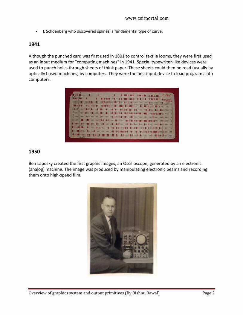
1951
The Whirlwind computer at the Massachusetts Institute of Technology was the first computer with a video display of real time data.
1955
The light pen is introduced.
1960
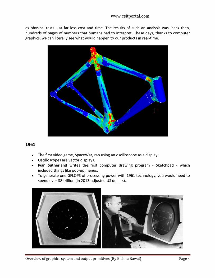
Although known since the 1940's, the first serious work on finite element methods of analysis is now published. FEA allows us to test products virtually and produce results that are as accurate
www.csitportal.com
Overview of graphics system and output primitives (By Bishnu Rawal) Page 4
as physical tests - at far less cost and time. The results of such an analysis was, back then, hundreds of pages of numbers that humans had to interpret. These days, thanks to computer graphics, we can literally see what would happen to our products in real-time.
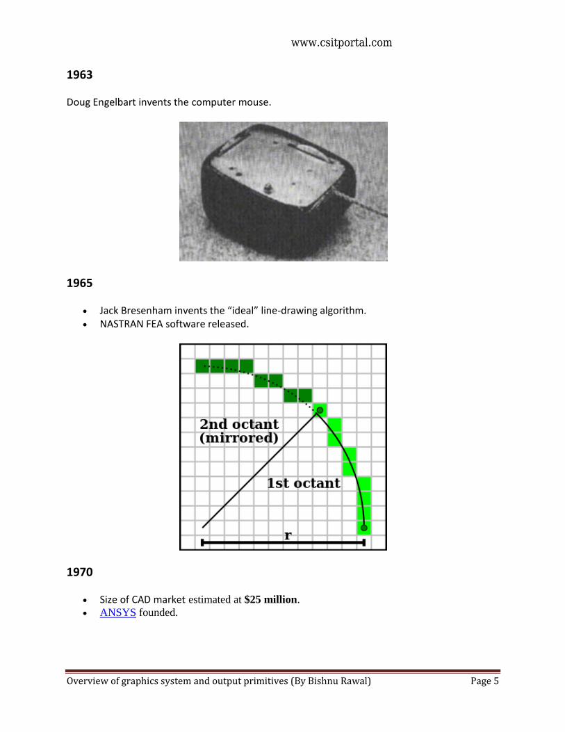
1961
The first video game, SpaceWar, ran using an oscilloscope as a display. Oscilloscopes are vector displays. Ivan Sutherland writes the first computer drawing program - Sketchpad - which
included things like pop-up menus. To generate one GFLOPS of processing power with 1961 technology, you would need to
spend over $8 trillion (in 2013-adjusted US dollars).
www.csitportal.com
Overview of graphics system and output primitives (By Bishnu Rawal) Page 5
1963
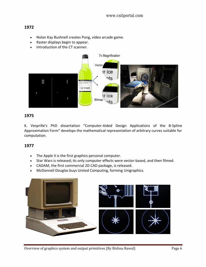
Doug Engelbart invents the computer mouse.
1965
Jack Bresenham invents the “ideal” line-drawing algorithm. NASTRAN FEA software released.
1970
Size of CAD market estimated at $25 million.
ANSYS founded.
www.csitportal.com
Overview of graphics system and output primitives (By Bishnu Rawal) Page 6
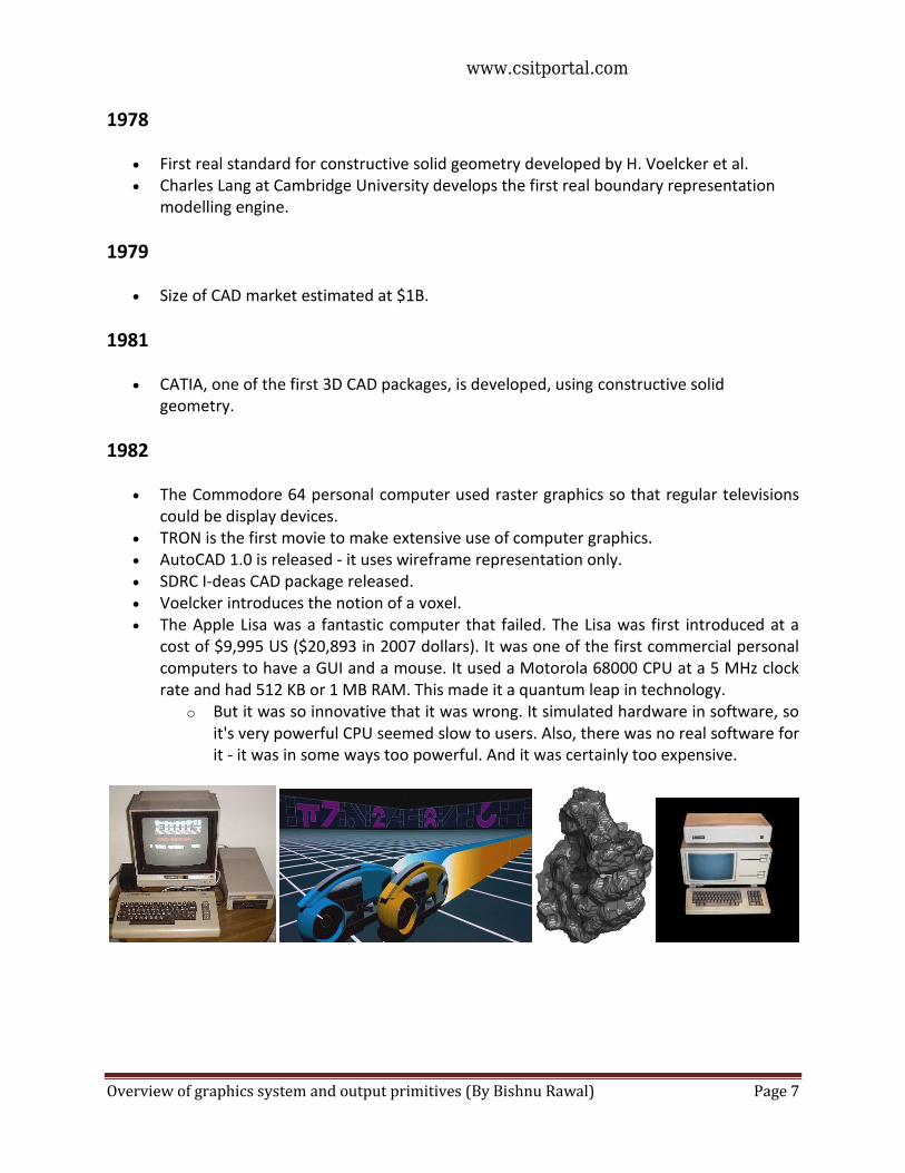
1972
Nolan Kay Bushnell creates Pong, video arcade game. Raster displays begin to appear. Introduction of the CT scanner.
1975
K. Vesprille's PhD dissertation “Computer-Aided Design Applications of the B-Spline Approximation Form” develops the mathematical representation of arbitrary curves suitable for computation.
1977
The Apple II is the first graphics personal computer. Star Wars is released; its only computer effects were vector-based, and then filmed. CADAM, the first commercial 2D CAD package, is released. McDonnell Douglas buys United Computing, forming Unigraphics.
www.csitportal.com
Overview of graphics system and output primitives (By Bishnu Rawal) Page 7
1978
First real standard for constructive solid geometry developed by H. Voelcker et al. Charles Lang at Cambridge University develops the first real boundary representation
modelling engine.
1979
Size of CAD market estimated at $1B.
1981
CATIA, one of the first 3D CAD packages, is developed, using constructive solid geometry.
1982
The Commodore 64 personal computer used raster graphics so that regular televisions could be display devices.
TRON is the first movie to make extensive use of computer graphics. AutoCAD 1.0 is released - it uses wireframe representation only. SDRC I-deas CAD package released. Voelcker introduces the notion of a voxel. The Apple Lisa was a fantastic computer that failed. The Lisa was first introduced at a
cost of $9,995 US ($20,893 in 2007 dollars). It was one of the first commercial personal computers to have a GUI and a mouse. It used a Motorola 68000 CPU at a 5 MHz clock rate and had 512 KB or 1 MB RAM. This made it a quantum leap in technology.
o But it was so innovative that it was wrong. It simulated hardware in software, so it's very powerful CPU seemed slow to users. Also, there was no real software for it - it was in some ways too powerful. And it was certainly too expensive.
www.csitportal.com
Overview of graphics system and output primitives (By Bishnu Rawal) Page 8
1984
To generate one GFLOPS of processing power, you would need to spend over $30 million in 2013-adjusted US dollars. (Compare that to the 1961 data.)
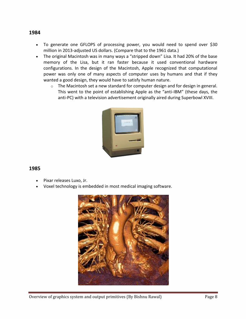
The original Macintosh was in many ways a “stripped down” Lisa. It had 20% of the base memory of the Lisa, but it ran faster because it used conventional hardware configurations. In the design of the Macintosh, Apple recognized that computational power was only one of many aspects of computer uses by humans and that if they wanted a good design, they would have to satisfy human nature.
o The Macintosh set a new standard for computer design and for design in general. This went to the point of establishing Apple as the “anti-IBM” (these days, the anti-PC) with a television advertisement originally aired during Superbowl XVIII.
1985
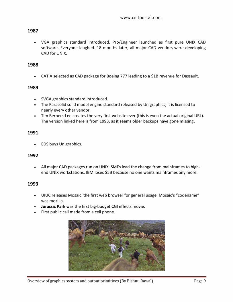
Pixar releases Luxo, Jr. Voxel technology is embedded in most medical imaging software.
Overview of graphics system and output primitives (By Bishnu Rawal) Page 9
1987
VGA graphics standard introduced. Pro/Engineer launched as first pure UNIX CAD software. Everyone laughed. 18 months later, all major CAD vendors were developing CAD for UNIX.
1988
CATIA selected as CAD package for Boeing 777 leading to a $1B revenue for Dassault.
1989
SVGA graphics standard introduced. The Parasolid solid model engine standard released by Unigraphics; it is licensed to
nearly every other vendor. Tim Berners-Lee creates the very first website ever (this is even the actual original URL).
The version linked here is from 1993, as it seems older backups have gone missing.
1991
EDS buys Unigraphics.
1992
All major CAD packages run on UNIX. SMEs lead the change from mainframes to high-end UNIX workstations. IBM loses $5B because no one wants mainframes any more.
1993
UIUC releases Mosaic, the first web browser for general usage. Mosaic's “codename” was mozilla.
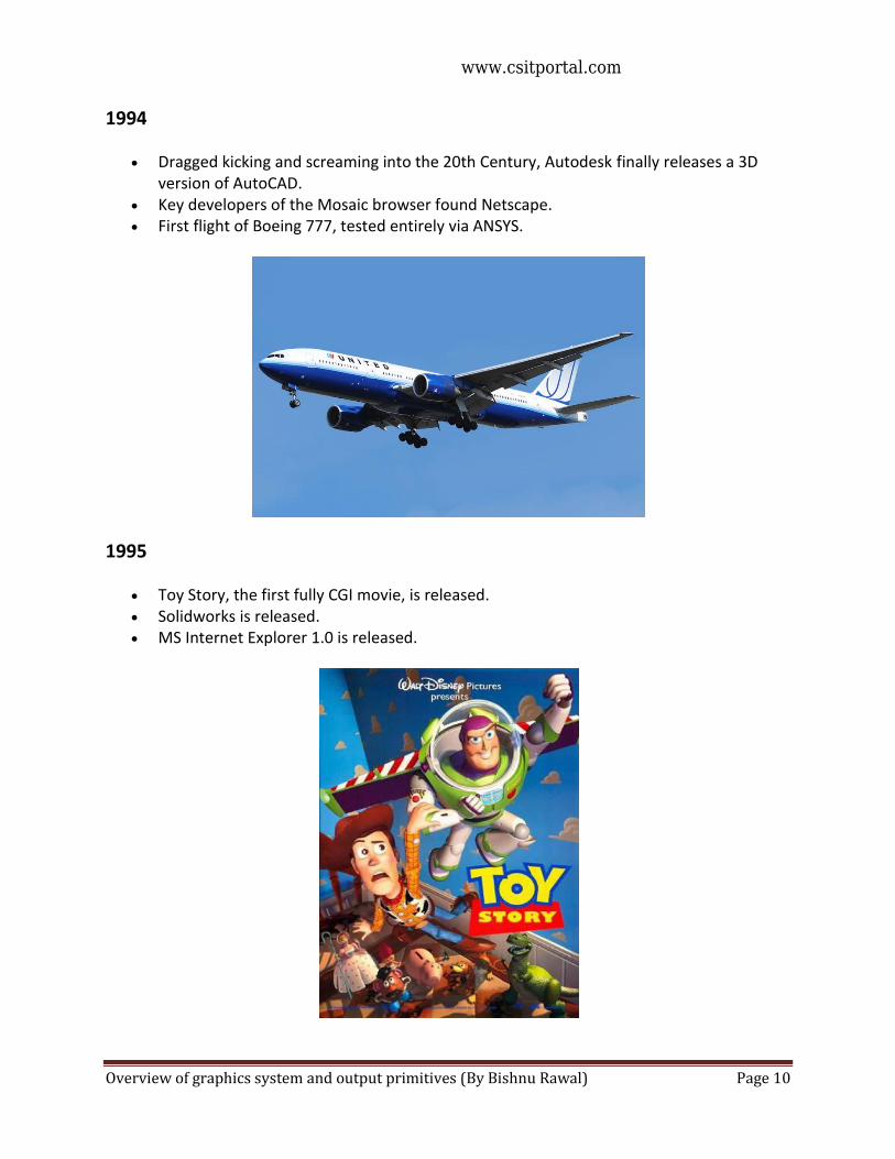
Jurassic Park was the first big-budget CGI effects movie. First public call made from a cell phone.
www.csitportal.com
Overview of graphics system and output primitives (By Bishnu Rawal) Page 10
1994
Dragged kicking and screaming into the 20th Century, Autodesk finally releases a 3D version of AutoCAD.
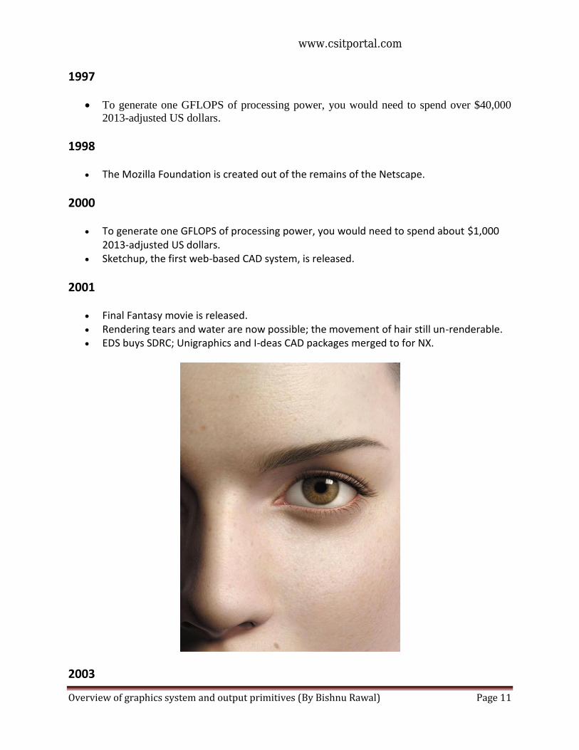
Key developers of the Mosaic browser found Netscape. First flight of Boeing 777, tested entirely via ANSYS.
1995
Toy Story, the first fully CGI movie, is released. Solidworks is released. MS Internet Explorer 1.0 is released.
www.csitportal.com
Overview of graphics system and output primitives (By Bishnu Rawal) Page 11
1997
To generate one GFLOPS of processing power, you would need to spend over $40,000
2013-adjusted US dollars.
1998
The Mozilla Foundation is created out of the remains of the Netscape.
2000
To generate one GFLOPS of processing power, you would need to spend about $1,000 2013-adjusted US dollars.
Sketchup, the first web-based CAD system, is released.
2001
Final Fantasy movie is released. Rendering tears and water are now possible; the movement of hair still un-renderable. EDS buys SDRC; Unigraphics and I-deas CAD packages merged to for NX.
2003
www.csitportal.com
Overview of graphics system and output primitives (By Bishnu Rawal) Page 12
Doom graphics engine for games. ANSYS acquires CFX - a computational fluid now begins to become popular. Mozilla.org is registered as a non-profit organization.
2006 Google acquires Sketchup.
2008 Mozilla.org opens an office in Toronto.
2009 The state of the art of computer graphics, as of 2009, is summarized in this YouTube
video URL: http://www.youtube.com/watch?v=qC5Y9W-E-po.
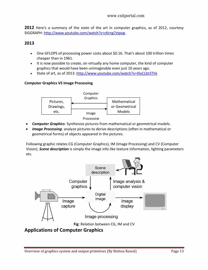
2010 Computations fluids and fluid structure interactions now possible on laptop PCs.
2011 One GFLOPS of processing power costs about $1.80.
www.csitportal.com
Overview of graphics system and output primitives (By Bishnu Rawal) Page 13
2012 Here's a summary of the state of the art in computer graphics, as of 2012, courtesy SIGGRAPH: http://www.youtube.com/watch?v=cKrng7ztpog.
2013
One GFLOPS of processing power costs about $0.16. That's about 100 trillion times cheaper than in 1961.
It is now possible to create, on virtually any home computer, the kind of computer graphics that would have been unimaginable even just 10 years ago.
State of art, as of 2013: http://www.youtube.com/watch?v=XlyCLbt3Thk
Computer Graphics VS Image Processing
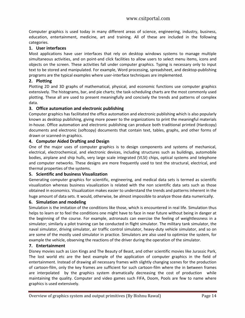
Computer Graphics: Synthesize pictures from mathematical or geometrical models.
Image Processing: analyze pictures to derive descriptions (often in mathematical or geometrical forms) of objects appeared in the pictures.
Following graphic relates CG (Computer Graphics), IM (Image Processing) and CV (Computer Vision). Scene description is simply the image info like texture information, lighting parameters etc.
Fig: Relation between CG, IM and CV
Applications of Computer Graphics
Pictures, Drawings,
etc.
Mathematical or Geometrical
Models
Computer Graphics
Image
Processing
www.csitportal.com
Overview of graphics system and output primitives (By Bishnu Rawal) Page 14
Computer graphics is used today in many different areas of science, engineering, industry, business, education, entertainment, medicine, art and training. All of these are included in the following categories.
1. User interfaces Most applications have user interfaces that rely on desktop windows systems to manage multiple simultaneous activities, and on point-and click facilities to allow users to select menu items, icons and objects on the screen. These activities fall under computer graphics. Typing is necessary only to input text to be stored and manipulated. For example, Word processing, spreadsheet, and desktop-publishing programs are the typical examples where user-interface techniques are implemented.
2. Plotting Plotting 2D and 3D graphs of mathematical, physical, and economic functions use computer graphics extensively. The histograms, bar, and pie charts; the task-scheduling charts are the most commonly used plotting. These all are used to present meaningfully and concisely the trends and patterns of complex data.
3. Office automation and electronic publishing Computer graphics has facilitated the office automation and electronic publishing which is also popularly known as desktop publishing, giving more power to the organizations to print the meaningful materials in-house. Office automation and electronic publishing can produce both traditional printed (Hardcopy) documents and electronic (softcopy) documents that contain text, tables, graphs, and other forms of drawn or scanned-in graphics.
4. Computer Aided Drafting and Design One of the major uses of computer graphics is to design components and systems of mechanical, electrical, electrochemical, and electronic devices, including structures such as buildings, automobile bodies, airplane and ship hulls, very large scale integrated (VLSI) chips, optical systems and telephone and computer networks. These designs are more frequently used to test the structural, electrical, and thermal properties of the systems.
5. Scientific and business Visualization Generating computer graphics for scientific, engineering, and medical data sets is termed as scientific visualization whereas business visualization is related with the non scientific data sets such as those obtained in economics. Visualization makes easier to understand the trends and patterns inherent in the
huge amount of data sets. It would, otherwise, be almost impossible to analyze those data numerically. 6. Simulation and modeling Simulation is the imitation of the conditions like those, which is encountered in real life. Simulation thus helps to learn or to feel the conditions one might have to face in near future without being in danger at the beginning of the course. For example, astronauts can exercise the feeling of weightlessness in a simulator; similarly a pilot training can be conducted in flight simulator. The military tank simulator, the naval simulator, driving simulator, air traffic control simulator, heavy-duty vehicle simulator, and so on are some of the mostly used simulator in practice. Simulators are also used to optimize the system, for example the vehicle, observing the reactions of the driver during the operation of the simulator. 7. Entertainment Disney movies such as Lion Kings and The Beauty of Beast, and other scientific movies like Jurassic Park, The lost world etc are the best example of the application of computer graphics in the field of entertainment. Instead of drawing all necessary frames with slightly changing scenes for the production of cartoon-film, only the key frames are sufficient for such cartoon-film where the in between frames are interpolated by the graphics system dramatically decreasing the cost of production while maintaining the quality. Computer and video games such FIFA, Doom, Pools are few to name where graphics is used extensively.
www.csitportal.com
Overview of graphics system and output primitives (By Bishnu Rawal) Page 15
8. Art and commerce Here computer graphics is used to produce pictures that express a message and attract attention such as a new model of a car moving along the ring of the Saturn. These pictures are frequently seen at transportation terminals supermarkets, hotels etc. The slide production for commercial, scientific, or educational presentations is another cost effective use of computer graphics. One of such graphics
packages is a PowerPoint. 9. Cartography Cartography is a subject, which deals with the making of maps and charts. Computer graphics is used to produce both accurate and schematic representations of geographical and other natural phenomena from measurement data. Examples include geographic maps, oceanographic charts, weather maps, contour maps and population-density maps. Surfer is one of such graphics packages, which is extensively used for cartography.
Graphics Hardware Systems
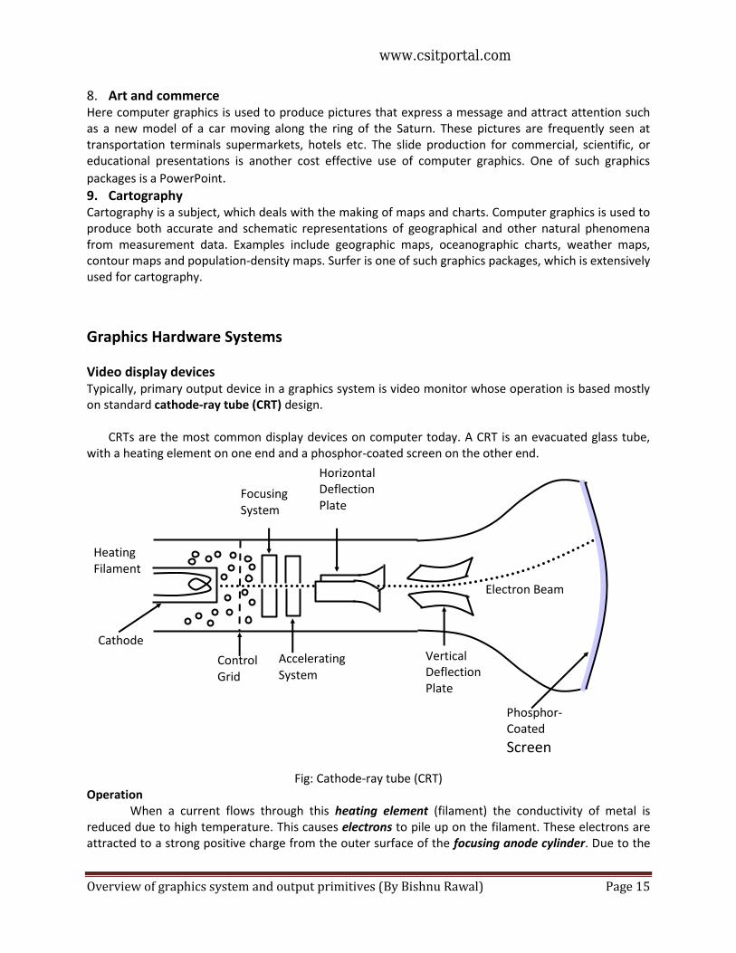
Video display devices Typically, primary output device in a graphics system is video monitor whose operation is based mostly on standard cathode-ray tube (CRT) design.
CRTs are the most common display devices on computer today. A CRT is an evacuated glass tube, with a heating element on one end and a phosphor-coated screen on the other end.
Fig: Cathode-ray tube (CRT)
Operation When a current flows through this heating element (filament) the conductivity of metal is
reduced due to high temperature. This causes electrons to pile up on the filament. These electrons are attracted to a strong positive charge from the outer surface of the focusing anode cylinder. Due to the
Horizontal Deflection Plate
Phosphor- Coated
Screen
Heating Filament
Control Grid
Accelerating System
Vertical Deflection Plate
Electron Beam
Focusing System
Cathode
www.csitportal.com
Overview of graphics system and output primitives (By Bishnu Rawal) Page 16
weaker negative charge inside the cylinder, the electrons head towards the anode forced into a beam and accelerated towards phosphor-coated screen by the high voltage in inner cylinder walls. The forwarding fast electron beam is called Cathode Ray.
There are two sets of weakly charged deflection plates with oppositely charged, one positive and another negative. The first set displaces the beam up and down and the second displaces the beam left and right. The electrons are sent flying out of the neck of bottle (tube) until the smash into the phosphor coating on the other end. When electrons strike on phosphor coating, the phosphor then emits a small spot of light at each position contacted by electron beam. The glowing positions are used to represent the picture in the screen. The amount of light emitted by the phosphor coating depends on the number of electrons striking the screen. The brightness of the display is controlled by varying the voltage on the control grid. Persistence How long a phosphor continues to emit light after the electron beam is removed?
− Persistence of phosphor is defined as time it takes for emitted light to decay to 1/10 (10%) of its original intensity. Range of persistence of different phosphors can react many seconds.
− Phosphors for graphical display have persistence of 10 to 60 microseconds. Phosphors with low persistence are useful for animation whereas high persistence phosphor is useful for highly complex, static pictures.
Refresh Rate
− Light emitted by phosphor fades very rapidly, so to keep the drawn picture glowing constantly; it is required to redraw the picture repeatedly and quickly directing the electron beam back over the some point. The no of times/sec the image is redrawn to give a feeling of non-flickering pictures is called refresh-rate.
− If Refresh rate decreases, flicker develops.
− Refresh rate above which flickering stops and steady it may be called as critical fusion frequency (CFF).
Resolution Maximum number of points displayed horizontally and vertically without overlap on a display screen is called resolution. More precise definition of resolution is no of dots per inch (dpi/pixel per inch) that can be plotted horizontally and vertically.
Color CRT A CRT monitor displays color pictures by using a combination of phosphors that emit different-
colored light. By combining the emitted light from the different phosphors, a range of colors can be generated. Two basic techniques for producing color displays with CRT are:
1. Beam-penetration method 2. Shadow-mask method
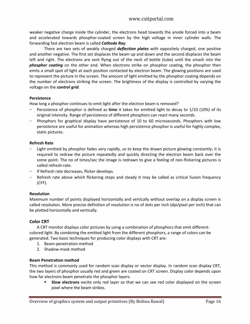
Beam Penetration method This method is commonly used for random scan display or vector display. In random scan display CRT, the two layers of phosphor usually red and green are coated on CRT screen. Display color depends upon how far electrons beam penetrate the phosphor layers.
Slow electrons excite only red layer so that we can see red color displayed on the screen pixel where the beam strikes.
www.csitportal.com
Overview of graphics system and output primitives (By Bishnu Rawal) Page 17
Fast electrons beam excite green layer penetrating the red layer and we can see the green color displayed at the corresponding position.
At Intermediate beam speeds, combinations of red and green light are emitted to show two additional colors - orange and yellow.
The speed of the electrons and hence the screen color at any point, is controlled by the beam-acceleration voltage.
Beam-penetration has an inexpensive way to produce color in random-scan monitors, but quality of pictures is not as good as other methods since only 4 colors are possible.
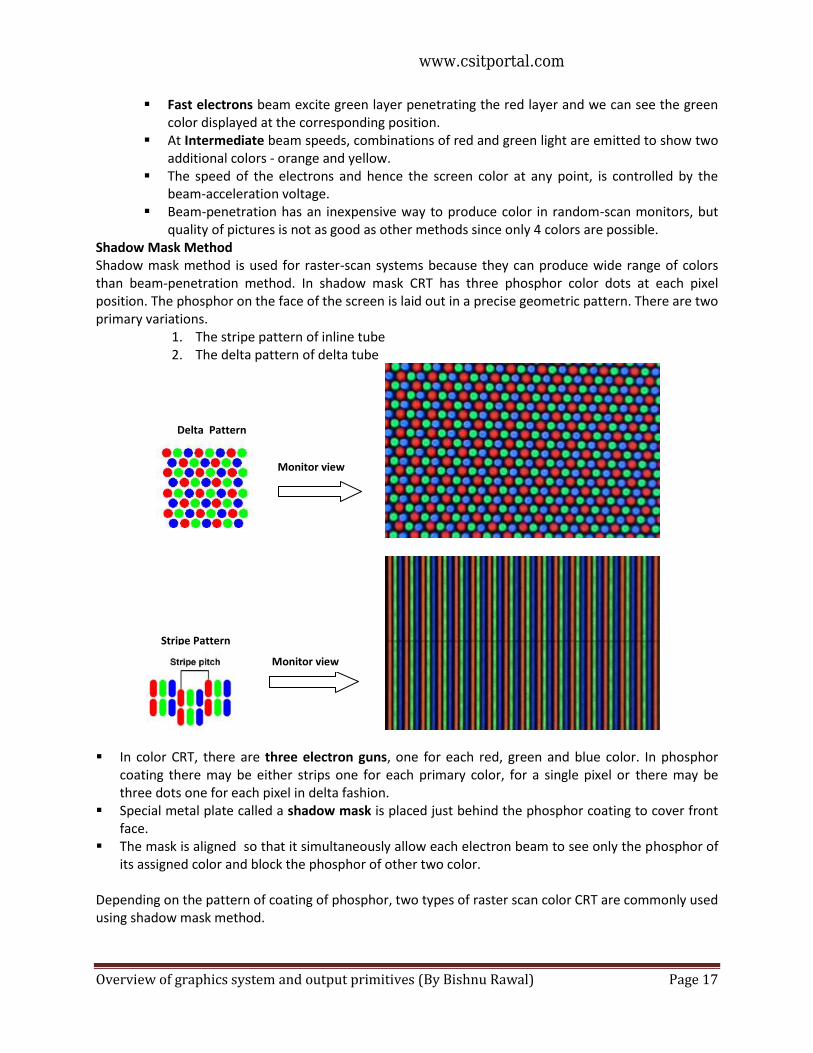
Shadow Mask Method Shadow mask method is used for raster-scan systems because they can produce wide range of colors than beam-penetration method. In shadow mask CRT has three phosphor color dots at each pixel position. The phosphor on the face of the screen is laid out in a precise geometric pattern. There are two primary variations.
1. The stripe pattern of inline tube 2. The delta pattern of delta tube
In color CRT, there are three electron guns, one for each red, green and blue color. In phosphor coating there may be either strips one for each primary color, for a single pixel or there may be three dots one for each pixel in delta fashion.
Special metal plate called a shadow mask is placed just behind the phosphor coating to cover front face.
The mask is aligned so that it simultaneously allow each electron beam to see only the phosphor of its assigned color and block the phosphor of other two color.
Depending on the pattern of coating of phosphor, two types of raster scan color CRT are commonly used using shadow mask method.
Monitor view
Monitor view
Delta Pattern
Stripe Pattern
www.csitportal.com
Overview of graphics system and output primitives (By Bishnu Rawal) Page 18
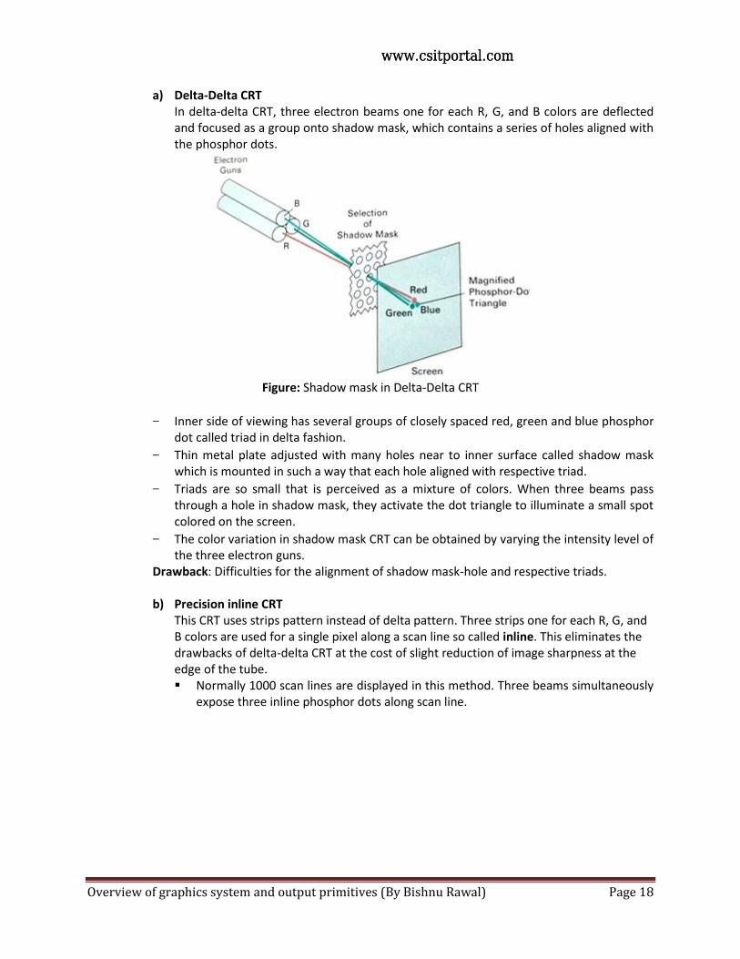
a) Delta-Delta CRT In delta-delta CRT, three electron beams one for each R, G, and B colors are deflected and focused as a group onto shadow mask, which contains a series of holes aligned with the phosphor dots.
Figure: Shadow mask in Delta-Delta CRT
− Inner side of viewing has several groups of closely spaced red, green and blue phosphor dot called triad in delta fashion.
− Thin metal plate adjusted with many holes near to inner surface called shadow mask which is mounted in such a way that each hole aligned with respective triad.
− Triads are so small that is perceived as a mixture of colors. When three beams pass through a hole in shadow mask, they activate the dot triangle to illuminate a small spot colored on the screen.
− The color variation in shadow mask CRT can be obtained by varying the intensity level of the three electron guns.
Drawback: Difficulties for the alignment of shadow mask-hole and respective triads.
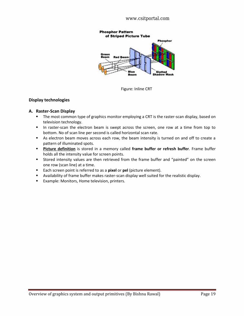
b) Precision inline CRT This CRT uses strips pattern instead of delta pattern. Three strips one for each R, G, and B colors are used for a single pixel along a scan line so called inline. This eliminates the drawbacks of delta-delta CRT at the cost of slight reduction of image sharpness at the edge of the tube. Normally 1000 scan lines are displayed in this method. Three beams simultaneously
expose three inline phosphor dots along scan line.
www.csitportal.comwww.csitportal.com
Overview of graphics system and output primitives (By Bishnu Rawal) Page 19
Figure: Inline CRT
Display technologies
A. Raster-Scan Display The most common type of graphics monitor employing a CRT is the raster-scan display, based on
television technology. In raster-scan the electron beam is swept across the screen, one row at a time from top to
bottom. No of scan line per second is called horizontal scan rate. As electron beam moves across each row, the beam intensity is turned on and off to create a
pattern of illuminated spots. Picture definition is stored in a memory called frame buffer or refresh buffer. Frame buffer
holds all the intensity value for screen points. Stored intensity values are then retrieved from the frame buffer and “painted” on the screen
one row (scan line) at a time. Each screen point is referred to as a pixel or pel (picture element). Availability of frame buffer makes raster-scan display well suited for the realistic display. Example: Monitors, Home television, printers.
www.csitportal.com
Overview of graphics system and output primitives (By Bishnu Rawal) Page 20
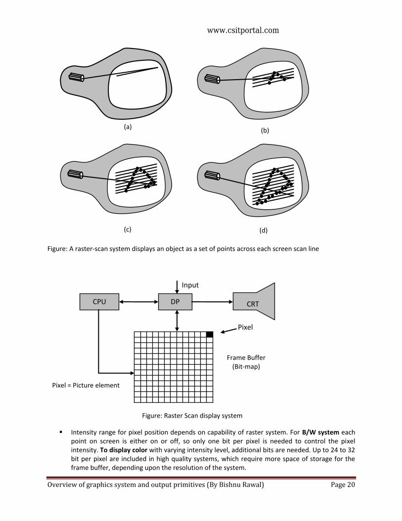
Figure: A raster-scan system displays an object as a set of points across each screen scan line
Figure: Raster Scan display system
Intensity range for pixel position depends on capability of raster system. For B/W system each point on screen is either on or off, so only one bit per pixel is needed to control the pixel intensity. To display color with varying intensity level, additional bits are needed. Up to 24 to 32 bit per pixel are included in high quality systems, which require more space of storage for the frame buffer, depending upon the resolution of the system.
Input
Pixel
CPU DP CRT
Frame Buffer (Bit-map)
Pixel = Picture element
(a) (b)
(d) (c)
www.csitportal.com
Overview of graphics system and output primitives (By Bishnu Rawal) Page 21
A system with 24 bit pixel and screen resolution 1024 1024 require 3 megabyte of storage in frame buffer.
1024*1024 pixels = 1024*1024*24 bits = 3 MB (using 24-bit per pixel)
The frame butter in B/W system stores a pixel with one bit per pixel so it is termed as bitmap. The frame buffer in multi bit per pixel storage is called pixmap.
Refreshing on Raster-Scan display is carried out at the rate of 60 or higher frames per second. Sometimes refresh rates are described in units of cycles per second or hertz (Hz), where cycle corresponds to one frame.
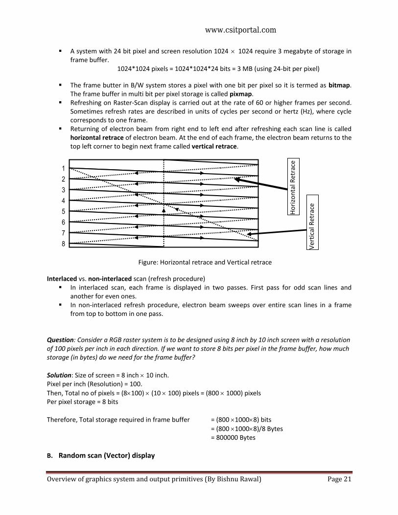
Returning of electron beam from right end to left end after refreshing each scan line is called horizontal retrace of electron beam. At the end of each frame, the electron beam returns to the top left corner to begin next frame called vertical retrace.
Figure: Horizontal retrace and Vertical retrace
Interlaced vs. non-interlaced scan (refresh procedure) In interlaced scan, each frame is displayed in two passes. First pass for odd scan lines and
another for even ones. In non-interlaced refresh procedure, electron beam sweeps over entire scan lines in a frame
from top to bottom in one pass. Question: Consider a RGB raster system is to be designed using 8 inch by 10 inch screen with a resolution of 100 pixels per inch in each direction. If we want to store 8 bits per pixel in the frame buffer, how much storage (in bytes) do we need for the frame buffer?
Solution: Size of screen = 8 inch 10 inch. Pixel per inch (Resolution) = 100.
Then, Total no of pixels = (8100) (10 100) pixels = (800 1000) pixels Per pixel storage = 8 bits
Therefore, Total storage required in frame buffer = (800 10008) bits
= (800 10008)/8 Bytes = 800000 Bytes
B. Random scan (Vector) display
1
2
3
4
5
6
7
8 Ver
tica
l Ret
race
Ho
rizo
nta
l Ret
race
www.csitportal.com
Overview of graphics system and output primitives (By Bishnu Rawal) Page 22
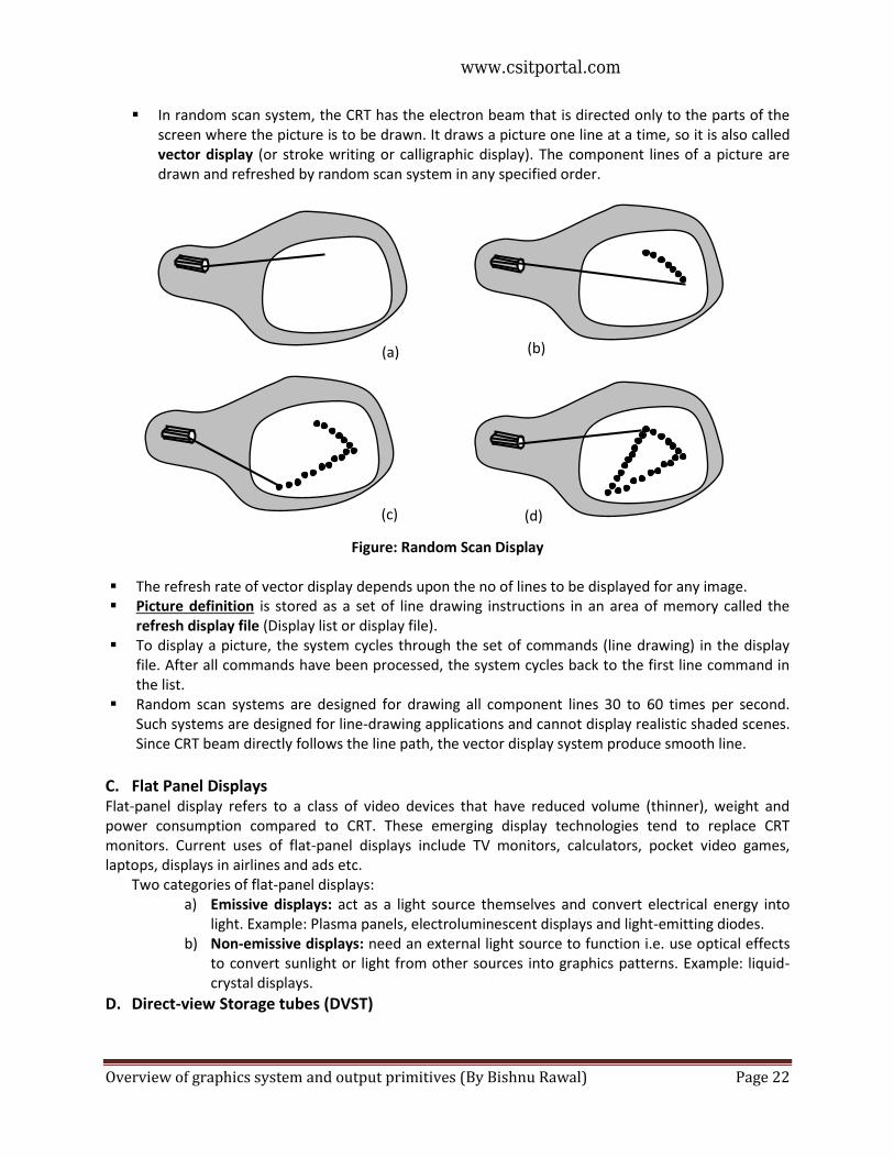
In random scan system, the CRT has the electron beam that is directed only to the parts of the screen where the picture is to be drawn. It draws a picture one line at a time, so it is also called vector display (or stroke writing or calligraphic display). The component lines of a picture are drawn and refreshed by random scan system in any specified order.
Figure: Random Scan Display The refresh rate of vector display depends upon the no of lines to be displayed for any image. Picture definition is stored as a set of line drawing instructions in an area of memory called the
refresh display file (Display list or display file). To display a picture, the system cycles through the set of commands (line drawing) in the display
file. After all commands have been processed, the system cycles back to the first line command in the list.
Random scan systems are designed for drawing all component lines 30 to 60 times per second. Such systems are designed for line-drawing applications and cannot display realistic shaded scenes. Since CRT beam directly follows the line path, the vector display system produce smooth line.
C. Flat Panel Displays Flat-panel display refers to a class of video devices that have reduced volume (thinner), weight and power consumption compared to CRT. These emerging display technologies tend to replace CRT monitors. Current uses of flat-panel displays include TV monitors, calculators, pocket video games, laptops, displays in airlines and ads etc.
Two categories of flat-panel displays: a) Emissive displays: act as a light source themselves and convert electrical energy into
light. Example: Plasma panels, electroluminescent displays and light-emitting diodes. b) Non-emissive displays: need an external light source to function i.e. use optical effects
to convert sunlight or light from other sources into graphics patterns. Example: liquid-crystal displays.
D. Direct-view Storage tubes (DVST)
(a) (b)
(c) (d)
www.csitportal.com
Overview of graphics system and output primitives (By Bishnu Rawal) Page 23
This is alternative method for method maintaining a screen image to store picture information inside the CRT instead of refreshing the system.
DVST stores the picture information as a charge distribution just behind the phosphor-coated screen.
Two electron guns used: primary gun – to store picture pattern and flood gun – maintains the picture display.
Pros: Since no refreshing is needed complex pictures can be displayed in high-resolution without flicker.
Cons: Ordinarily do not display color and that selected parts of picture can not be erased. To eliminate a picture section, entire screen must be erased and modified picture redrawn, which may take several seconds for complex picture.
Hey! For details of flat displays, read page no. 65-67 of book “Computer graphics C version”, Hearn & Baker.
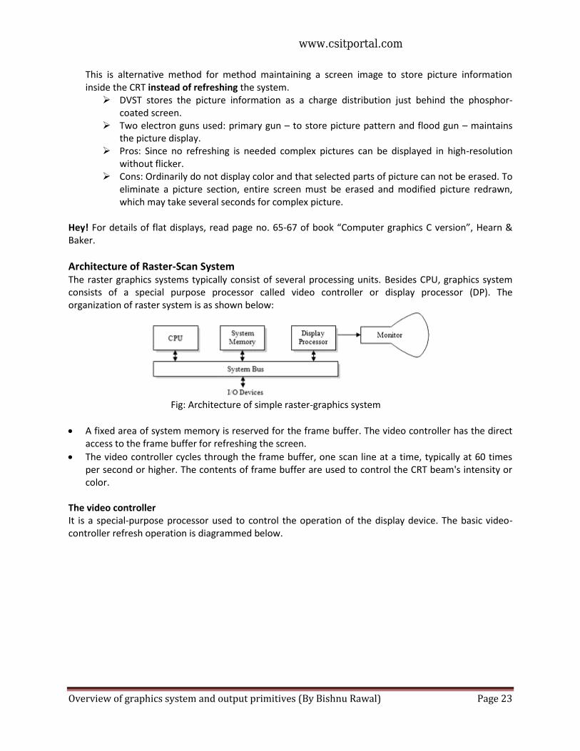
Architecture of Raster-Scan System The raster graphics systems typically consist of several processing units. Besides CPU, graphics system consists of a special purpose processor called video controller or display processor (DP). The organization of raster system is as shown below:
Fig: Architecture of simple raster-graphics system
A fixed area of system memory is reserved for the frame buffer. The video controller has the direct access to the frame buffer for refreshing the screen.
The video controller cycles through the frame buffer, one scan line at a time, typically at 60 times per second or higher. The contents of frame buffer are used to control the CRT beam's intensity or color.
The video controller It is a special-purpose processor used to control the operation of the display device. The basic video-controller refresh operation is diagrammed below.
www.csitportal.com
Overview of graphics system and output primitives (By Bishnu Rawal) Page 24
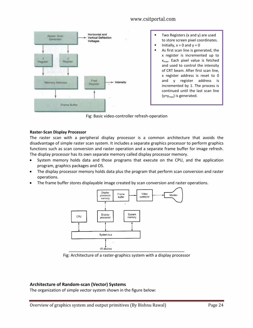
Fig: Basic video-controller refresh-operation
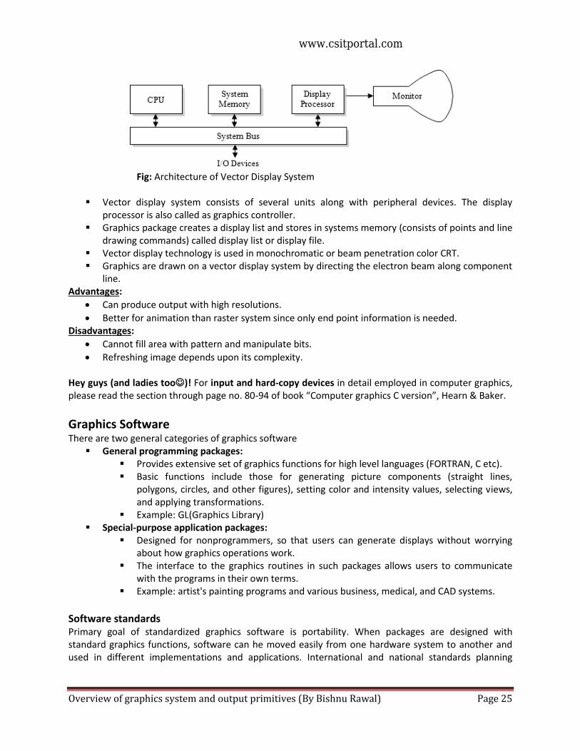
Raster-Scan Display Processor The raster scan with a peripheral display processor is a common architecture that avoids the disadvantage of simple raster scan system. It includes a separate graphics processor to perform graphics functions such as scan conversion and raster operation and a separate frame buffer for image refresh. The display processor has its own separate memory called display processor memory.
System memory holds data and those programs that execute on the CPU, and the application program, graphics packages and OS.
The display processor memory holds data plus the program that perform scan conversion and raster operations.
The frame buffer stores displayable image created by scan conversion and raster operations.
Fig: Architecture of a raster-graphics system with a display processor
Architecture of Random-scan (Vector) Systems The organization of simple vector system shown in the figure below:
Two Registers (x and y) are used to store screen pixel coordinates.
Initially, x = 0 and y = 0 As first scan line is generated, the
x register is incremented up to xmax. Each pixel value is fetched and used to control the intensity of CRT beam. After first scan line, x register address is reset to 0 and y register address is incremented by 1. The process is continued until the last scan line (y=ymax) is generated.
www.csitportal.com
Overview of graphics system and output primitives (By Bishnu Rawal) Page 25
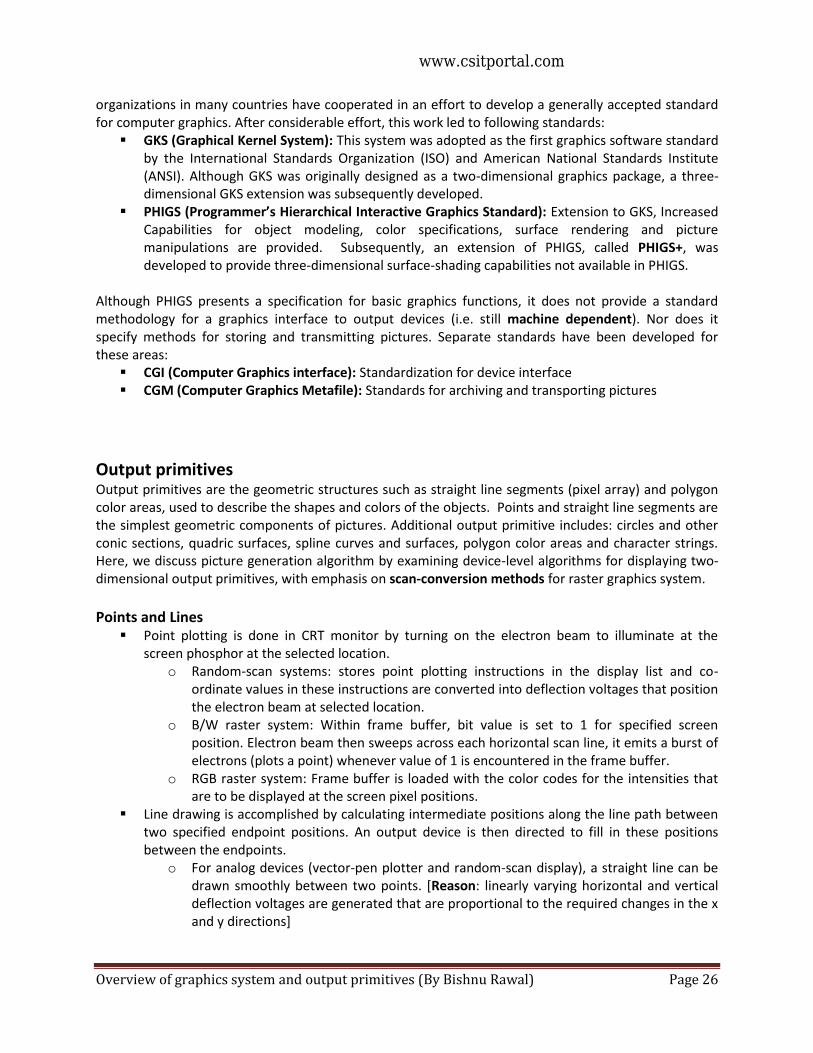
Fig: Architecture of Vector Display System
Vector display system consists of several units along with peripheral devices. The display processor is also called as graphics controller.
Graphics package creates a display list and stores in systems memory (consists of points and line drawing commands) called display list or display file.
Vector display technology is used in monochromatic or beam penetration color CRT. Graphics are drawn on a vector display system by directing the electron beam along component
line. Advantages:
Can produce output with high resolutions.
Better for animation than raster system since only end point information is needed. Disadvantages:
Cannot fill area with pattern and manipulate bits.
Refreshing image depends upon its complexity. Hey guys (and ladies too)! For input and hard-copy devices in detail employed in computer graphics, please read the section through page no. 80-94 of book “Computer graphics C version”, Hearn & Baker.
Graphics Software There are two general categories of graphics software
General programming packages: Provides extensive set of graphics functions for high level languages (FORTRAN, C etc). Basic functions include those for generating picture components (straight lines,
polygons, circles, and other figures), setting color and intensity values, selecting views, and applying transformations.
Example: GL(Graphics Library) Special-purpose application packages:
Designed for nonprogrammers, so that users can generate displays without worrying about how graphics operations work.
The interface to the graphics routines in such packages allows users to communicate with the programs in their own terms.
Example: artist's painting programs and various business, medical, and CAD systems.
Software standards Primary goal of standardized graphics software is portability. When packages are designed with standard graphics functions, software can he moved easily from one hardware system to another and used in different implementations and applications. International and national standards planning
www.csitportal.com
Overview of graphics system and output primitives (By Bishnu Rawal) Page 26
organizations in many countries have cooperated in an effort to develop a generally accepted standard for computer graphics. After considerable effort, this work led to following standards:
GKS (Graphical Kernel System): This system was adopted as the first graphics software standard by the International Standards Organization (ISO) and American National Standards Institute (ANSI). Although GKS was originally designed as a two-dimensional graphics package, a three-dimensional GKS extension was subsequently developed.
PHIGS (Programmer’s Hierarchical Interactive Graphics Standard): Extension to GKS, Increased Capabilities for object modeling, color specifications, surface rendering and picture manipulations are provided. Subsequently, an extension of PHIGS, called PHIGS+, was developed to provide three-dimensional surface-shading capabilities not available in PHIGS.
Although PHIGS presents a specification for basic graphics functions, it does not provide a standard methodology for a graphics interface to output devices (i.e. still machine dependent). Nor does it specify methods for storing and transmitting pictures. Separate standards have been developed for these areas:
CGI (Computer Graphics interface): Standardization for device interface CGM (Computer Graphics Metafile): Standards for archiving and transporting pictures
Output primitives Output primitives are the geometric structures such as straight line segments (pixel array) and polygon color areas, used to describe the shapes and colors of the objects. Points and straight line segments are the simplest geometric components of pictures. Additional output primitive includes: circles and other conic sections, quadric surfaces, spline curves and surfaces, polygon color areas and character strings. Here, we discuss picture generation algorithm by examining device-level algorithms for displaying two-dimensional output primitives, with emphasis on scan-conversion methods for raster graphics system.
Points and Lines
Point plotting is done in CRT monitor by turning on the electron beam to illuminate at the screen phosphor at the selected location.
o Random-scan systems: stores point plotting instructions in the display list and co-ordinate values in these instructions are converted into deflection voltages that position the electron beam at selected location.
o B/W raster system: Within frame buffer, bit value is set to 1 for specified screen position. Electron beam then sweeps across each horizontal scan line, it emits a burst of electrons (plots a point) whenever value of 1 is encountered in the frame buffer.
o RGB raster system: Frame buffer is loaded with the color codes for the intensities that are to be displayed at the screen pixel positions.
Line drawing is accomplished by calculating intermediate positions along the line path between two specified endpoint positions. An output device is then directed to fill in these positions between the endpoints.
o For analog devices (vector-pen plotter and random-scan display), a straight line can be drawn smoothly between two points. [Reason: linearly varying horizontal and vertical deflection voltages are generated that are proportional to the required changes in the x and y directions]
www.csitportal.com
Overview of graphics system and output primitives (By Bishnu Rawal) Page 27
o Digital devices display a straight line segment by plotting discrete points between two end-points. Discrete integer coordinates are calculated from the equation of the line. Since rounding of coordinate values occur [viz. (4.48, 48.51) would be converted to (4, 49)], line is displayed with stairstep appearance.
Line Drawing Algorithms The Cartesian slope-intercept equation of a straight line is
bmxy …..…… (1), where m = slope of line and b = y-intercept.
For any two given points ),( 11 yx and ),( 22 yx of a line segment, we can determine m and b with
following calculations:
m = 12
12
xx
yy
(1) becomes,
yb xxx
yy
12
12
At any point ),( kk yx ,
bmxy kk …………………….. (2)
At ),( 11 kk yx ,
bmxy kk 11 ……………………… (3)
Subtracting (2) from (3) we get,
)( 11 kkkk xxmyy
Here ( kk yy 1 ) is increment in y as corresponding increment in x.
xmy .
or x
ym
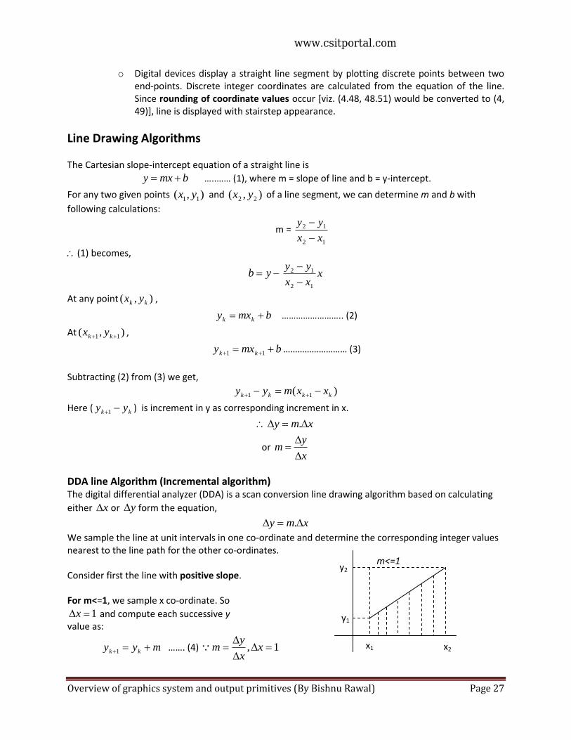
DDA line Algorithm (Incremental algorithm) The digital differential analyzer (DDA) is a scan conversion line drawing algorithm based on calculating
either x or y form the equation,
xmy .
We sample the line at unit intervals in one co-ordinate and determine the corresponding integer values nearest to the line path for the other co-ordinates. Consider first the line with positive slope. For m<=1, we sample x co-ordinate. So
1x and compute each successive y value as:
myy kk 1 ……. (4) 1,
x
x
ym
y1
y2
x1
m<=1
x2
www.csitportal.com
Overview of graphics system and output primitives (By Bishnu Rawal) Page 28
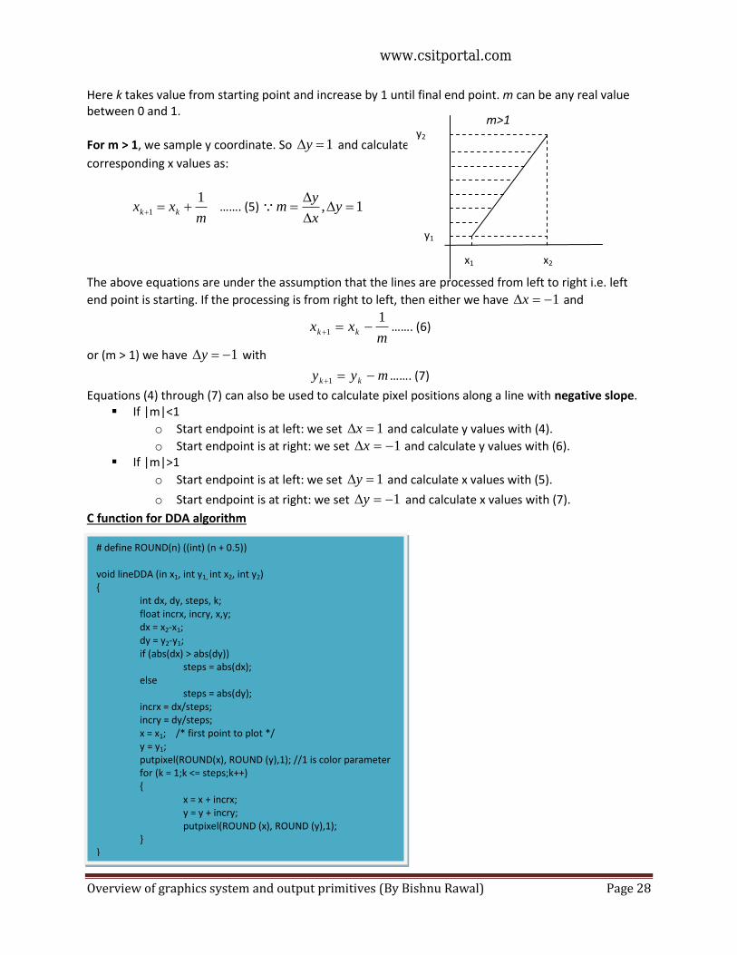
Here k takes value from starting point and increase by 1 until final end point. m can be any real value between 0 and 1.
For m > 1, we sample y coordinate. So 1y and calculate
corresponding x values as:
mxx kk
11 ……. (5) 1,
y
x
ym
The above equations are under the assumption that the lines are processed from left to right i.e. left
end point is starting. If the processing is from right to left, then either we have 1x and
mxx kk
11 ……. (6)
or (m > 1) we have 1y with
myy kk 1 ……. (7)
Equations (4) through (7) can also be used to calculate pixel positions along a line with negative slope. If |m|<1
o Start endpoint is at left: we set 1x and calculate y values with (4).
o Start endpoint is at right: we set 1x and calculate y values with (6). If |m|>1
o Start endpoint is at left: we set 1y and calculate x values with (5).
o Start endpoint is at right: we set 1y and calculate x values with (7).
C function for DDA algorithm
y2
y1
x1 x2
m>1
# define ROUND(n) ((int) (n + 0.5)) void lineDDA (in x1, int y1, int x2, int y2) { int dx, dy, steps, k; float incrx, incry, x,y; dx = x2-x1; dy = y2-y1; if (abs(dx) > abs(dy)) steps = abs(dx); else steps = abs(dy); incrx = dx/steps; incry = dy/steps; x = x1; /* first point to plot */ y = y1; putpixel(ROUND(x), ROUND (y),1); //1 is color parameter for (k = 1;k <= steps;k++) { x = x + incrx; y = y + incry; putpixel(ROUND (x), ROUND (y),1); } }
www.csitportal.com
Overview of graphics system and output primitives (By Bishnu Rawal) Page 29
The DDA algorithm is faster method for calculating pixel position than direct use of line equation but it has problems:
Accumulation of roundoff error in successive additions can cause calculated pixel positions to drift away from the actual line path for long line segments.
Rounding operations and floating-point-arithmetic are time consuming.
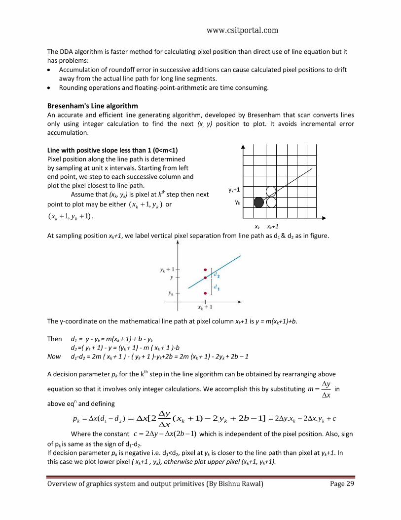
Bresenham's Line algorithm An accurate and efficient line generating algorithm, developed by Bresenham that scan converts lines only using integer calculation to find the next (x, y) position to plot. It avoids incremental error accumulation. Line with positive slope less than 1 (0<m<1) Pixel position along the line path is determined by sampling at unit x intervals. Starting from left end point, we step to each successive column and plot the pixel closest to line path. Assume that (xk, yk) is pixel at kth
step then next
point to plot may be either ),1( kk yx or
)1,1( kk yx .
At sampling position xk+1, we label vertical pixel separation from line path as d1 & d2 as in figure.
The y-coordinate on the mathematical line path at pixel column xk+1 is y = m(xk+1)+b.
Then d1 = y - yk = m(xk + 1) + b - yk
d2 =( yk + 1) - y = (yk + 1) - m ( xk + 1 )-b Now d1-d2 = 2m ( xk + 1 ) - ( yk + 1 )-yk+2b = 2m (xk + 1) - 2yk + 2b – 1 A decision parameter pk for the kth step in the line algorithm can be obtained by rearranging above
equation so that it involves only integer calculations. We accomplish this by substituting x
ym
in
above eqn and defining
)( 21 ddxpk ]122)1(2[
byx
x
yx kk cyxxy kk .2.2
Where the constant )12(2 bxyc which is independent of the pixel position. Also, sign
of pk is same as the sign of d1-d2. If decision parameter pk is negative i.e. d1<d2, pixel at yk is closer to the line path than pixel at yk+1. In this case we plot lower pixel ( xk+1 , yk), otherwise plot upper pixel (xk+1, yk+1).
xk xk+1
yk+1
yk
www.csitportal.com
Overview of graphics system and output primitives (By Bishnu Rawal) Page 30
Co-ordinate change along the line occur in unit steps in either x, or y direction. Therefore we can obtain the values of successive decision parameters using incremental integer calculations. At step k+1, decision parameter pk+1 is evaluated as.
cxyxyp kkk 111 2.2
)(2)(2 111 kkkkkk yyxxxypp
Since 11 kk xx
)(22 11 kkkk yyxypp
The term kk yy 1 is either 0 or 1 depending upon the sign of .kp
The first decision parameter p0 is evaluated as xypo 2
and successively we can calculate decision parameter as )(22 11 kkkk yyxypp
So if pk is negative, yk+1 = yk so pk+1 = pk+ 2 y
Otherwise yk+1 = yk+1, then pk+1 = pk+ 2 y -2 x
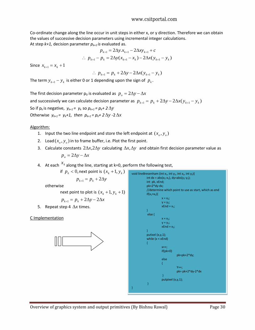
Algorithm:
1. Input the two line endpoint and store the left endpoint at ),( oo yx
2. Load ),( oo yx in to frame buffer, i.e. Plot the first point.
3. Calculate constants yx 2,2 calculating yx , and obtain first decision parameter value as
xypo 2
4. At each kxalong the line, starting at k=0, perform the following test,
if ,0kp next point is ),1( kk yx
ypp kk 21
otherwise
next point to plot is )1,1( kk yx
xypp kk 221
5. Repeat step 4 x times. C Implementation
void lineBresenham (int x1, int y1, int x2, int y2){ int dx = abs(x2-x1), dy=abs(y2-y1);
int pk, xEnd; pk=2*dy-dx; //determine which point to use as start, which as end if(x1>x2){
x = x2; y = y2; xEnd = x1; } else { x = x1; y = y1; xEnd = x2; } putixel (x,y,1); while (x < xEnd)
{ x++;
if(pk<0) pk=pk+2*dy; else
{ Y++; pk= pk+2*dy-2*dx } putpixel (x,y,1);
} }
www.csitportal.com
Overview of graphics system and output primitives (By Bishnu Rawal) Page 31
Bresenham’s algorithm is generalized to lines with arbitrary slope by considering the symmetry between the various octants & quadrants of xy-plane. Line with positive slope greater than 1 (m>1) Here, we simply interchange the role of x & y in the above procedure i.e. we step along the y-direction in unit steps and calculate successive x values nearest the line path.
Circle generating algorithms Circle is a frequently used component in pictures and graphs, a procedure for generating circular arcs or full circles is included in most graphics packages.
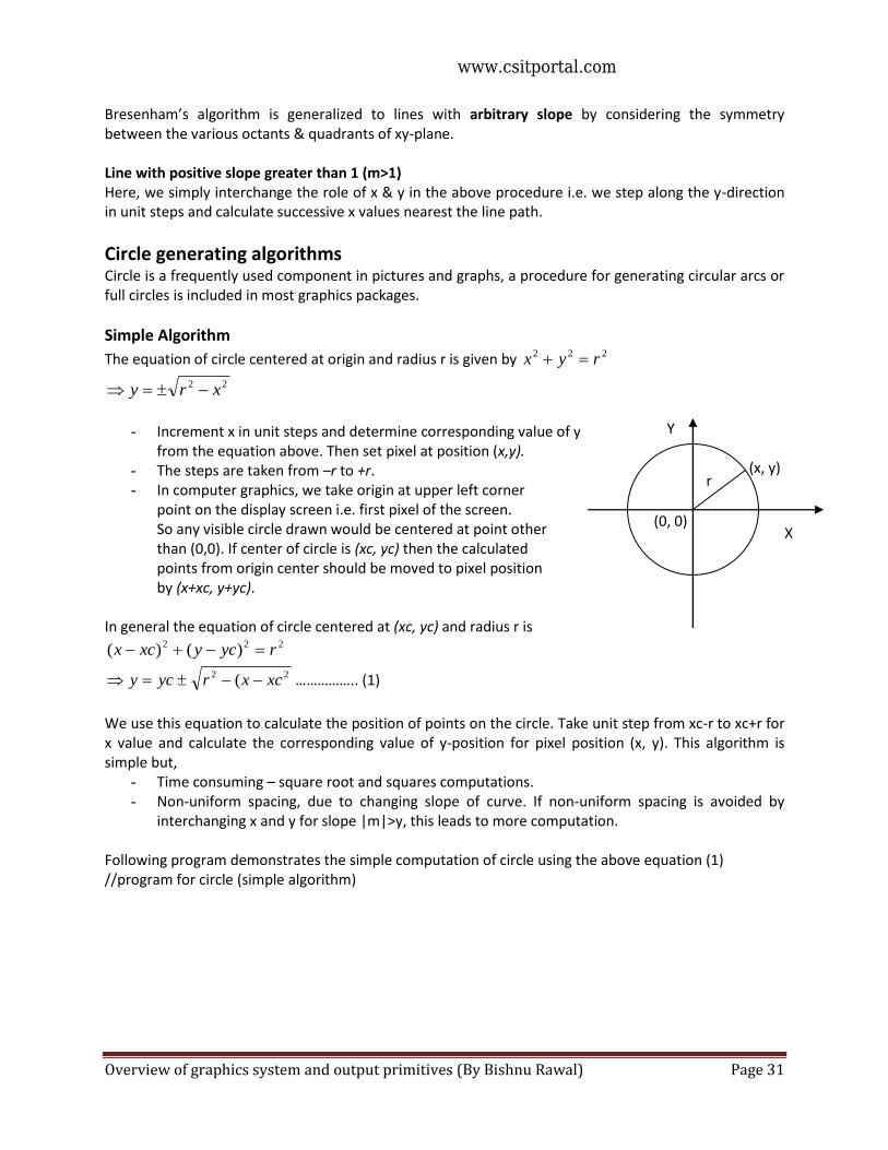
Simple Algorithm
The equation of circle centered at origin and radius r is given by 222ryx
22xry
- Increment x in unit steps and determine corresponding value of y
from the equation above. Then set pixel at position (x,y). - The steps are taken from –r to +r. - In computer graphics, we take origin at upper left corner
point on the display screen i.e. first pixel of the screen. So any visible circle drawn would be centered at point other than (0,0). If center of circle is (xc, yc) then the calculated points from origin center should be moved to pixel position by (x+xc, y+yc).
In general the equation of circle centered at (xc, yc) and radius r is 222
)()( rycyxcx
22( xcxrycy …………….. (1)
We use this equation to calculate the position of points on the circle. Take unit step from xc-r to xc+r for x value and calculate the corresponding value of y-position for pixel position (x, y). This algorithm is simple but,
- Time consuming – square root and squares computations. - Non-uniform spacing, due to changing slope of curve. If non-uniform spacing is avoided by
interchanging x and y for slope |m|>y, this leads to more computation. Following program demonstrates the simple computation of circle using the above equation (1) //program for circle (simple algorithm)
Y
X
r (x, y)
(0, 0)
www.csitportal.com
Overview of graphics system and output primitives (By Bishnu Rawal) Page 32
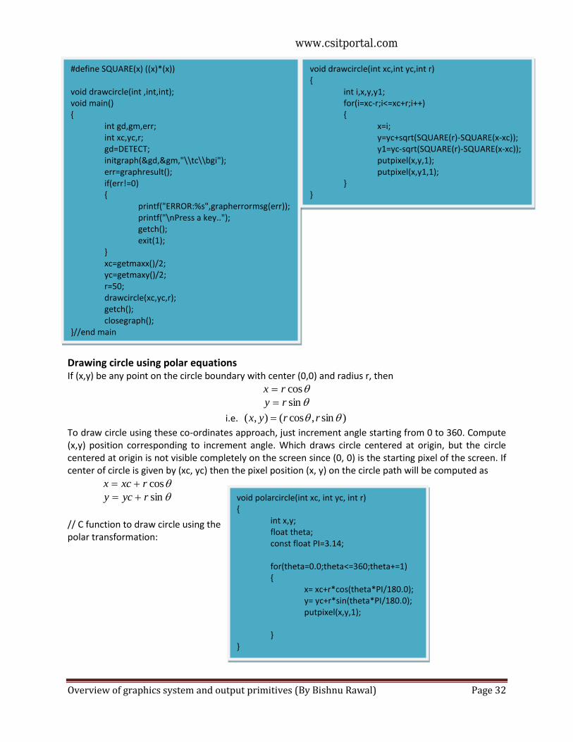
Drawing circle using polar equations If (x,y) be any point on the circle boundary with center (0,0) and radius r, then
cosrx
sinry
i.e. )sin,cos(),( rryx
To draw circle using these co-ordinates approach, just increment angle starting from 0 to 360. Compute (x,y) position corresponding to increment angle. Which draws circle centered at origin, but the circle centered at origin is not visible completely on the screen since (0, 0) is the starting pixel of the screen. If center of circle is given by (xc, yc) then the pixel position (x, y) on the circle path will be computed as
cosrxcx
sinrycy
// C function to draw circle using the polar transformation:
#define SQUARE(x) ((x)*(x)) void drawcircle(int ,int,int); void main() { int gd,gm,err; int xc,yc,r; gd=DETECT; initgraph(&gd,&gm,"\\tc\\bgi"); err=graphresult(); if(err!=0) { printf("ERROR:%s",grapherrormsg(err)); printf("\nPress a key.."); getch(); exit(1); } xc=getmaxx()/2; yc=getmaxy()/2; r=50; drawcircle(xc,yc,r); getch(); closegraph(); }//end main
void drawcircle(int xc,int yc,int r) { int i,x,y,y1; for(i=xc-r;i<=xc+r;i++) { x=i; y=yc+sqrt(SQUARE(r)-SQUARE(x-xc)); y1=yc-sqrt(SQUARE(r)-SQUARE(x-xc)); putpixel(x,y,1); putpixel(x,y1,1); } }
void polarcircle(int xc, int yc, int r) { int x,y; float theta; const float PI=3.14; for(theta=0.0;theta<=360;theta+=1) { x= xc+r*cos(theta*PI/180.0); y= yc+r*sin(theta*PI/180.0); putpixel(x,y,1); } }
www.csitportal.com
Overview of graphics system and output primitives (By Bishnu Rawal) Page 33
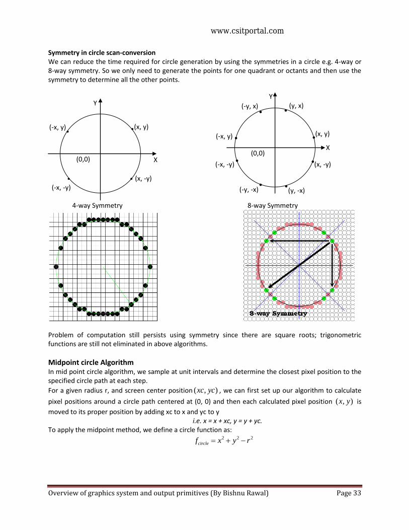
Symmetry in circle scan-conversion We can reduce the time required for circle generation by using the symmetries in a circle e.g. 4-way or 8-way symmetry. So we only need to generate the points for one quadrant or octants and then use the symmetry to determine all the other points.
4-way Symmetry 8-way Symmetry
Problem of computation still persists using symmetry since there are square roots; trigonometric functions are still not eliminated in above algorithms.
Midpoint circle Algorithm In mid point circle algorithm, we sample at unit intervals and determine the closest pixel position to the specified circle path at each step.
For a given radius r, and screen center position ),( ycxc , we can first set up our algorithm to calculate
pixel positions around a circle path centered at (0, 0) and then each calculated pixel position ),( yx is
moved to its proper position by adding xc to x and yc to y i.e. x = x + xc, y = y + yc.
To apply the midpoint method, we define a circle function as:
222ryxfcircle
Y
X
(x, y)
(0,0)
Y
X (0,0)
●
●
●
●
(x, -y) (-x, -y)
(-x, y)
●
●
●
●
●
●
●
●
(x, y)
(y, x)
(x, -y)
(y, -x) (-y, -x)
(-x, -y)
(-x, y)
(-y, x)
www.csitportal.com
Overview of graphics system and output primitives (By Bishnu Rawal) Page 34
To summarize the relative position of point ),( yx by checking sign of circlef function,
<0, if ),( yx lies inside the circle boundary
),( yxfcircle =0, if ),( yx lies on the circle boundary
>0, if ),( yx lies outside the circle boundary.
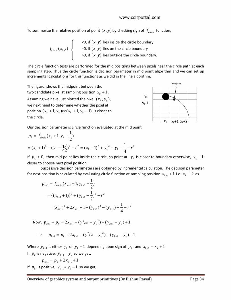
The circle function tests are performed for the mid positions between pixels near the circle path at each sampling step. Thus the circle function is decision parameter in mid point algorithm and we can set up incremental calculations for this functions as we did in the line algorithm. The figure, shows the midpoint between the
two candidate pixel at sampling position 1kx ,
Assuming we have just plotted the pixel ),,( kk yx
we next need to determine whether the pixel at
position )1,1(),1( kkkk yxoryx is closer to
the circle. Our decision parameter is circle function evaluated at the mid point
)2
1,1( kkcirclek yxfp
222222
4
1)1()
21()1( ryyxryx kkkkk
If ,0kp then mid-point lies inside the circle, so point at ky is closer to boundary otherwise, 1ky
closer to choose next pixel position. Successive decision parameters are obtained by incremental calculation. The decision parameter
for next position is calculated by evaluating circle function at sampling position 11 kx i.e. 2kx as
)2
1,1( 111 kkcirclek yxfp
22
1
2
1 )2
1()}1{( ryx kk
2
1
2
11
2
14
1)()(12)( ryyxx kkkk
Now, 1)()(2 1
21
2
11 kkkkkkk yyyyxpp
i.e. 1)()(2 1
21
2
11 kkkkkkk yyyyxpp
Where 1ky is either ky or 1ky depending upon sign of .kp and 11 kk xx
If kp is negative, 1ky = ky so we get,
12 11 kkk xpp
If kp is positive, 1ky = 1ky so we get,
yk
yk-1
xk+1 xk
Mid point
xk+2
www.csitportal.com
Overview of graphics system and output primitives (By Bishnu Rawal) Page 35
111 212 kkkk yxpp
Where 222 1 kk xx
222 1 kk yy
At the start position, (0, r), these two terms have the values 0 and 2r, respectively. Each successive values are obtained by adding 2 to the previous value of 2x and subtracting 2 from previous value of 2y. The initial decision parameter is obtained by evaluating the circle function at starting position
)2
1,1(0 rfp circle
22)
21(1 rr
22
4
11 rrr
If 0p is specified in integer,
.10 rp
Steps of Mid-point circle algorithm
1. Input radius r and circle centre ),( cc yx and obtain the first point on circle centered at origin as.
2. Calculate initial decision parameter
rp 4
50
3. At each kx position, starting at ,0k perform the tests:
If 0kp next point along the circle centre at )0,0( is ),1( kk yx
)12 11 kkk xpp
Otherwise, the next point along circle is )1,1( kk yx
111 212 kkkk yxpp
Where .222 1 kk xx and .222 1 kk yy
4. Determine symmetry point on the other seven octants.
5. Move each calculated pixels positions ),( yx in to circle path centered at ),( cc yx as
cc yyyxxx ,
6. Repeat 3 through 5 until .yx
).,0(),( 00 ryx
r4
5
).,0(),( 00 ryx
www.csitportal.com
Overview of graphics system and output primitives (By Bishnu Rawal) Page 36
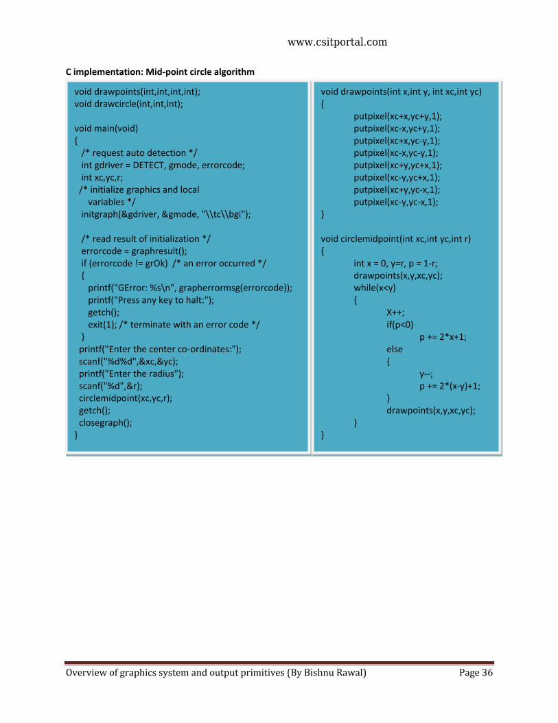
C implementation: Mid-point circle algorithm
void drawpoints(int,int,int,int); void drawcircle(int,int,int); void main(void) { /* request auto detection */ int gdriver = DETECT, gmode, errorcode; int xc,yc,r; /* initialize graphics and local variables */ initgraph(&gdriver, &gmode, "\\tc\\bgi"); /* read result of initialization */ errorcode = graphresult(); if (errorcode != grOk) /* an error occurred */ { printf("GError: %s\n", grapherrormsg(errorcode)); printf("Press any key to halt:"); getch(); exit(1); /* terminate with an error code */ } printf("Enter the center co-ordinates:"); scanf("%d%d",&xc,&yc); printf("Enter the radius"); scanf("%d",&r); circlemidpoint(xc,yc,r); getch(); closegraph(); }
void drawpoints(int x,int y, int xc,int yc) { putpixel(xc+x,yc+y,1); putpixel(xc-x,yc+y,1); putpixel(xc+x,yc-y,1); putpixel(xc-x,yc-y,1); putpixel(xc+y,yc+x,1); putpixel(xc-y,yc+x,1); putpixel(xc+y,yc-x,1); putpixel(xc-y,yc-x,1); } void circlemidpoint(int xc,int yc,int r) { int x = 0, y=r, p = 1-r; drawpoints(x,y,xc,yc); while(x<y) { X++; if(p<0) p += 2*x+1; else { y--; p += 2*(x-y)+1; } drawpoints(x,y,xc,yc); } }
www.csitportal.com
Overview of graphics system and output primitives (By Bishnu Rawal) Page 37
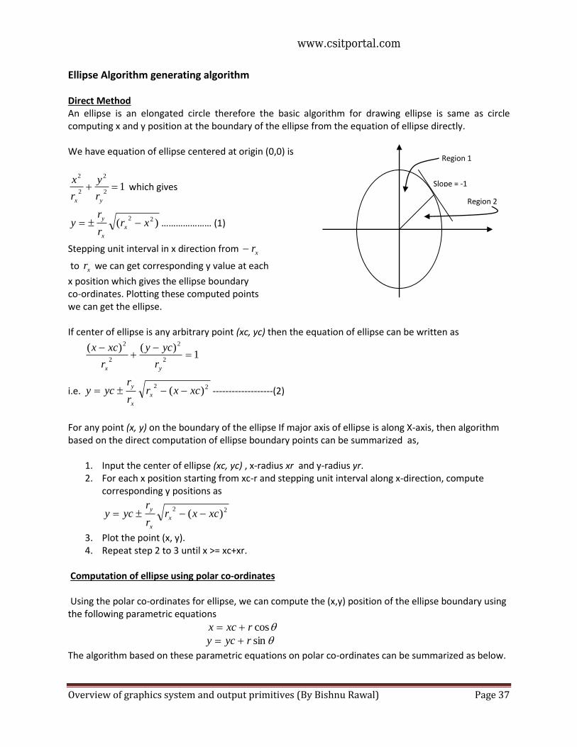
Ellipse Algorithm generating algorithm Direct Method An ellipse is an elongated circle therefore the basic algorithm for drawing ellipse is same as circle computing x and y position at the boundary of the ellipse from the equation of ellipse directly. We have equation of ellipse centered at origin (0,0) is
12
2
2
2
yx r
y
r
x which gives
)(22
xrr
ry x
x
y ………………… (1)
Stepping unit interval in x direction from xr
to xr we can get corresponding y value at each
x position which gives the ellipse boundary co-ordinates. Plotting these computed points we can get the ellipse. If center of ellipse is any arbitrary point (xc, yc) then the equation of ellipse can be written as
1)()(
2
2
2
2
yx r
ycy
r
xcx
i.e. 22
)( xcxrr
rycy x
x
y -------------------(2)
For any point (x, y) on the boundary of the ellipse If major axis of ellipse is along X-axis, then algorithm based on the direct computation of ellipse boundary points can be summarized as,
1. Input the center of ellipse (xc, yc) , x-radius xr and y-radius yr. 2. For each x position starting from xc-r and stepping unit interval along x-direction, compute
corresponding y positions as
22)( xcxr
r
rycy x
x
y
3. Plot the point (x, y). 4. Repeat step 2 to 3 until x >= xc+xr.
Computation of ellipse using polar co-ordinates Using the polar co-ordinates for ellipse, we can compute the (x,y) position of the ellipse boundary using the following parametric equations
cosrxcx
sinrycy
The algorithm based on these parametric equations on polar co-ordinates can be summarized as below.
Figure
Region 1
Region 2
Slope = -1
rx
ry
www.csitportal.com
Overview of graphics system and output primitives (By Bishnu Rawal) Page 38
1. Input center of ellipse (xc,yc) and radii xr and yr.
2. Starting from angle 0o step minimum increments and compute boundary point of ellipse as
cosrxcx
sinrycy
3. Plot the point at position (round(x), round(y))
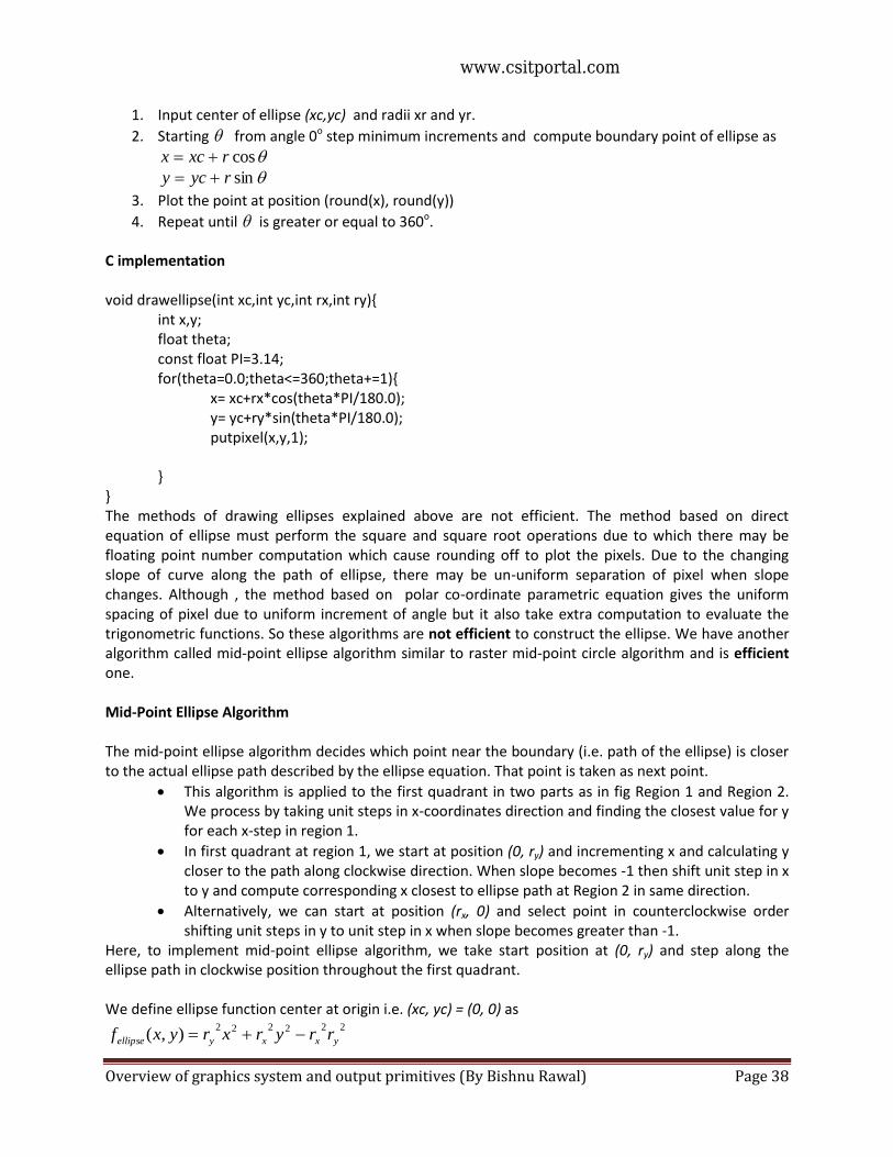
4. Repeat until is greater or equal to 360o. C implementation void drawellipse(int xc,int yc,int rx,int ry){ int x,y; float theta; const float PI=3.14; for(theta=0.0;theta<=360;theta+=1){ x= xc+rx*cos(theta*PI/180.0); y= yc+ry*sin(theta*PI/180.0); putpixel(x,y,1); } } The methods of drawing ellipses explained above are not efficient. The method based on direct equation of ellipse must perform the square and square root operations due to which there may be floating point number computation which cause rounding off to plot the pixels. Due to the changing slope of curve along the path of ellipse, there may be un-uniform separation of pixel when slope changes. Although , the method based on polar co-ordinate parametric equation gives the uniform spacing of pixel due to uniform increment of angle but it also take extra computation to evaluate the trigonometric functions. So these algorithms are not efficient to construct the ellipse. We have another algorithm called mid-point ellipse algorithm similar to raster mid-point circle algorithm and is efficient one. Mid-Point Ellipse Algorithm The mid-point ellipse algorithm decides which point near the boundary (i.e. path of the ellipse) is closer to the actual ellipse path described by the ellipse equation. That point is taken as next point.
This algorithm is applied to the first quadrant in two parts as in fig Region 1 and Region 2. We process by taking unit steps in x-coordinates direction and finding the closest value for y for each x-step in region 1.
In first quadrant at region 1, we start at position (0, ry) and incrementing x and calculating y closer to the path along clockwise direction. When slope becomes -1 then shift unit step in x to y and compute corresponding x closest to ellipse path at Region 2 in same direction.
Alternatively, we can start at position (rx, 0) and select point in counterclockwise order shifting unit steps in y to unit step in x when slope becomes greater than -1.
Here, to implement mid-point ellipse algorithm, we take start position at (0, ry) and step along the ellipse path in clockwise position throughout the first quadrant. We define ellipse function center at origin i.e. (xc, yc) = (0, 0) as
222222),( yxxyellipse rryrxryxf
www.csitportal.com
Overview of graphics system and output primitives (By Bishnu Rawal) Page 39
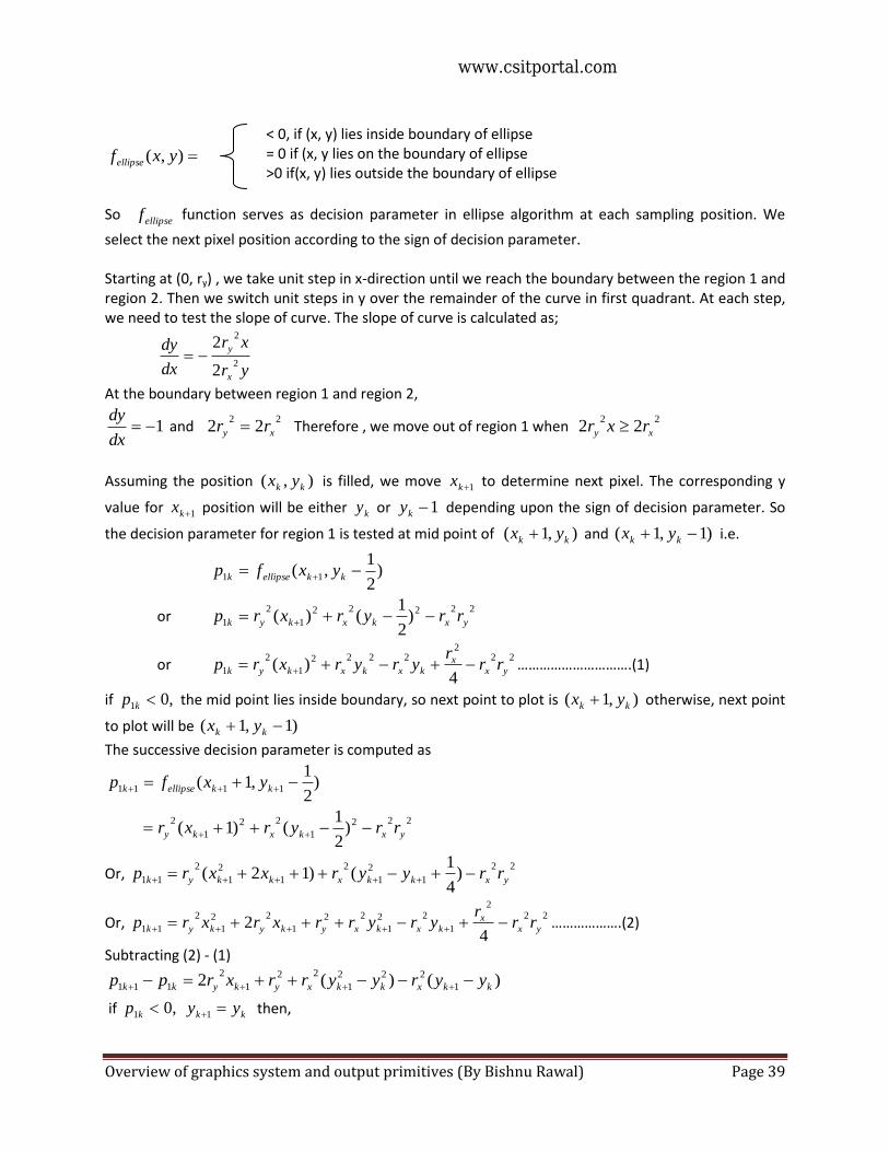
< 0, if (x, y) lies inside boundary of ellipse = 0 if (x, y lies on the boundary of ellipse
>0 if(x, y) lies outside the boundary of ellipse
So ellipsef function serves as decision parameter in ellipse algorithm at each sampling position. We
select the next pixel position according to the sign of decision parameter. Starting at (0, ry) , we take unit step in x-direction until we reach the boundary between the region 1 and region 2. Then we switch unit steps in y over the remainder of the curve in first quadrant. At each step, we need to test the slope of curve. The slope of curve is calculated as;
yr
xr
dx
dy
x
y
2
2
2
2
At the boundary between region 1 and region 2,
1dx
dy and
2222 xy rr Therefore , we move out of region 1 when
2222 xy rxr
Assuming the position ),( kk yx is filled, we move 1kx to determine next pixel. The corresponding y
value for 1kx position will be either ky or 1ky depending upon the sign of decision parameter. So
the decision parameter for region 1 is tested at mid point of ),1( kk yx and )1,1( kk yx i.e.
)2
1,( 11 kkellipsek yxfp
or 22222
1
2
1 )2
1()( yxkxkyk rryrxrp
or 22
22222
1
2
14
)( yxx
kxkxkyk rrr
yryrxrp ………………………….(1)
if ,01 kp the mid point lies inside boundary, so next point to plot is ),1( kk yx otherwise, next point
to plot will be )1,1( kk yx
The successive decision parameter is computed as
)2
1,1( 1111 kkellipsek yxfp
222
1
22
1
2)
2
1()1( yxkxky rryrxr
Or, 22
1
2
1
2
1
2
1
2
11 )4
1()12( yxkkxkkyk rryyrxxrp
Or, 22
2
1
22
1
22
1
22
1
2
114
2 yxx
kxkxykykyk rrr
yryrrxrxrp ……………….(2)
Subtracting (2) - (1)
)()(2 1
222
1
22
1
2
111 kkxkkxykykk yyryyrrxrpp
if ,01 kp kk yy 1 then,
),( yxfellipse
www.csitportal.com
Overview of graphics system and output primitives (By Bishnu Rawal) Page 40
2
1
2
111 2 ykykk rxrpp
Otherwise 11 kk yy then we get,
1
22
1
2
111 22 kxykykk yrrxrpp
At the initial position, (0, ry) 022
xry and
yxx rryr22
22
In region 1, initial decision parameter is obtained by evaluating ellipse function at (0, ry) as
)2
1,1(10 yellipse rfp
Or, )2
1,1(10 yellipse rfp
222
4
1xyxy rrrr
Similarly, over the region 2, the decision parameter is tested at mid point of )1,( kk yx and
)1,1( kk yx i.e.
)1,2
1(2 kkellipsek yxfp
222222)1()
2
1( yxkxky rryrxr
2222
2
222
2 )1(4
yxkx
y
kykyk rryrr
xrxrp …………….(3)
if ,02 kp the mid point lies outside the boundary, so next point to plot is )1,( kk yx otherwise, next
point to plot will be )1,1( kk yx
The successive decision parameter is computed as evaluating ellipse function at mid point of
)1,2
1( 1112 kkellipsek yxfp with yk+1= yk-1
22222
1
2
12 ]1)1[()2
1( yxkxkyk rryrxrp
Or 222222
2
1
22
1
2
12 )1(2)1(4
yxxkxkx
y
kykyk rrryryrr
xrxrp ……….(4)
Subtracting (4)-(3)
22
1
222
1
2
212 )1(2)()( xkxkkykkykk ryrxxrxxrpp
www.csitportal.com
Overview of graphics system and output primitives (By Bishnu Rawal) Page 41
Or 22
1
222
1
2
212 )1(2)()( xkxkkykkykk ryrxxrxxrpp
if ,02 kp kk xx 1 then 22
212 )1(2 xkxkk ryrpp Otherwise 11 kk xx then
222222
212 )1(2)1()])1[( xkxkkykkykk ryrxxrxxrpp
Or, 2222
212 )1(2)12( xkxykykk ryrrxrpp
Or, 222
212 )1(2)22( xkxkykk ryrxrpp
Or, 2
1
2
1
2
212 22 xkxkykk ryrxrpp where 11 kk xx and 11 kk yy
The initial position for region 2 is taken as last position selected in region 1 say which is (x0, y0) then initial decision parameter in region 2 is obtained by evaluating ellipse function at mid point of (x0,y0-1) and (x0 +1,y0-1) as
)1,2
1( 0020 yxfp ellipse
222
0
22
0
2)1()
2
1( yxxy rryrxr
Now the mid point ellipse algorithm is summarized as;
1. Input center (xc, yc) and rx and ry for the ellipse and obtain the first point as (x0,y0) =(0,ry) 2. Calculate initial decision parameter value in Region 1 as
222
104
1xyxy rrrrP
3. At each xk position, in Region 1, starting at k = 0 , compute xk+1 = 1kx
If ,01 kp then the next point to plot is
2
1
2
111 2 ykykk rxrpp
yk+1 = yk
Otherwise next point to plot is
, yk+1 = 1ky
1
22
1
2
111 22 kxykykk yrrxrpp with xk+1 = xk + 1 and yk+1 = yk - 1
4. Calculate the initial value of decision parameter at region 2 using last calculated point say (x0,y0) in region 1 as
222
0
22
0
2
20 )1()2
1( yxxy rryrxrp
5. At each yk position in Region 2 starting at k = 0, perform computation yk+1 = y-1;
if ,02 kp then
xk+1 = xk
22
212 )1(2 xkxkk ryrpp
Otherwise xk+1 = xk +1
2
1
2
1
2
212 22 xkxkykk ryrxrpp where 11 kk xx and 11 kk yy
www.csitportal.com
Overview of graphics system and output primitives (By Bishnu Rawal) Page 42
6. Determine the symmetry points in other 3 quadrants. 7. Move each calculated point (xk, yk) on to the centered (xc,yc) ellipse path as
xk = xk + xc; yk = yk + yc
8. Repeat the process for region 1 until kxky yrxr
2222 and region until (xk, yk) =(rx,0)
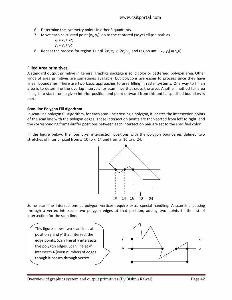
Filled Area primitives A standard output primitive in general graphics package is solid color or patterned polygon area. Other kinds of area primitives are sometimes available, but polygons are easier to process since they have linear boundaries. There are two basic approaches to area filling in raster systems. One way to fill an area is to determine the overlap intervals for scan lines that cross the area. Another method for area filling is to start from a given interior position and point outward from this until a specified boundary is met. Scan-line Polygon Fill Algorithm In scan-line polygon fill algorithm, for each scan-line crossing a polygon, it locates the intersection points of the scan line with the polygon edges. These intersection points are then sorted from left to right, and the corresponding frame-buffer positions between each intersection pair are set to the specified color. In the figure below, the four pixel intersection positions with the polygon boundaries defined two stretches of interior pixel from x=10 to x=14 and from x=16 to x=24. Some scan-line intersections at polygon vertices require extra special handling. A scan-line passing through a vertex intersects two polygon edges at that position, adding two points to the list of intersection for the scan-line.
y'
y
L1
L2
10 14 16 18 24
This figure shows two scan lines at
position y and y' that intersect the
edge points. Scan line at y intersects
five polygon edges. Scan line at y'
intersects 4 (even number) of edges
though it passes through vertex.
www.csitportal.com
Overview of graphics system and output primitives (By Bishnu Rawal) Page 43
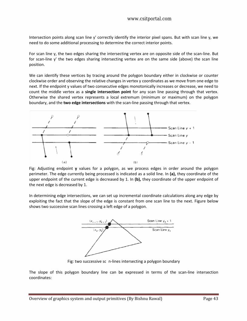
Intersection points along scan line y' correctly identify the interior pixel spans. But with scan line y, we need to do some additional processing to determine the correct interior points. For scan line y, the two edges sharing the intersecting vertex are on opposite side of the scan-line. But for scan-line y' the two edges sharing intersecting vertex are on the same side (above) the scan line position. We can identify these vertices by tracing around the polygon boundary either in clockwise or counter clockwise order and observing the relative changes in vertex y coordinates as we move from one edge to next. If the endpoint y values of two consecutive edges monotonically increases or decrease, we need to count the middle vertex as a single intersection point for any scan line passing through that vertex. Otherwise the shared vertex represents a local extremum (minimum or maximum) on the polygon boundary, and the two edge intersections with the scan-line passing through that vertex.
Fig: Adjusting endpoint y values for a polygon, as we process edges in order around the polygon perimeter. The edge currently being processed is indicated as a solid line. In (a), they coordinate of the upper endpoint of the current edge is decreased by 1. In (b), they coordinate of the upper endpoint of the next edge is decreased by 1. In determining edge intersections, we can set up incremental coordinate calculations along any edge by exploiting the fact that the slope of the edge is constant from one scan line to the next. Figure below shows two successive scan lines crossing a left edge of a polygon.
Fig: two successive scan-lines intersecting a polygon boundary
The slope of this polygon boundary line can be expressed in terms of the scan-line intersection coordinates:
www.csitportal.com
Overview of graphics system and output primitives (By Bishnu Rawal) Page 44
kk
kk
xx
yym
1
1 .
Since the change between two scan line in y co-ordinates is 1,
11 kk yy
The x-intersection value ,1kx on the upper scan line can be determined from the x-intersection value
,kx on the preceding scan line as
m
xx kk1
1
Each successive x-intercept can thus be calculated by adding the inverse of the slope and rounding to the nearest integer recalling that the slope m is the ratio to two integers
x
ym
Where yx & are the differences between the edge endpoint x and y co-ordinate values. Thus
incremental calculations of x intercepts along an edge for successive scan lines can be expressed as
.
1y
xxx kk
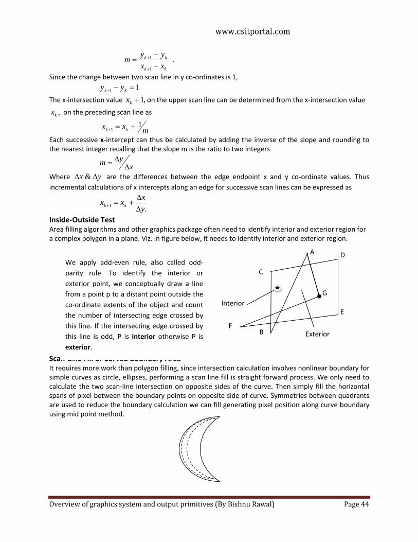
Inside-Outside Test Area filling algorithms and other graphics package often need to identify interior and exterior region for a complex polygon in a plane. Viz. in figure below, it needs to identify interior and exterior region.
Scan-Line Fill of Curved Boundary Area It requires more work than polygon filling, since intersection calculation involves nonlinear boundary for simple curves as circle, ellipses, performing a scan line fill is straight forward process. We only need to calculate the two scan-line intersection on opposite sides of the curve. Then simply fill the horizontal spans of pixel between the boundary points on opposite side of curve. Symmetries between quadrants are used to reduce the boundary calculation we can fill generating pixel position along curve boundary using mid point method.
C
A D
G
E
B F
Exterior
Interior
We apply add-even rule, also called odd-
parity rule. To identify the interior or
exterior point, we conceptually draw a line
from a point p to a distant point outside the
co-ordinate extents of the object and count
the number of intersecting edge crossed by
this line. If the intersecting edge crossed by
this line is odd, P is interior otherwise P is
exterior.
www.csitportal.com
Overview of graphics system and output primitives (By Bishnu Rawal) Page 45
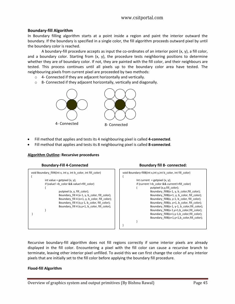
Boundary-fill Algorithm In Boundary filling algorithm starts at a point inside a region and paint the interior outward the boundary. If the boundary is specified in a single color, the fill algorithm proceeds outward pixel by until the boundary color is reached. A boundary-fill procedure accepts as input the co-ordinates of an interior point (x, y), a fill color, and a boundary color. Starting from (x, y), the procedure tests neighboring positions to determine whether they are of boundary color. If not, they are painted with the fill color, and their neighbours are tested. This process continues until all pixels up to the boundary color area have tested. The neighbouring pixels from current pixel are proceeded by two methods:
o 4- Connected if they are adjacent horizontally and vertically. o 8- Connected if they adjacent horizontally, vertically and diagonally.
Fill method that applies and tests its 4 neighbouring pixel is called 4-connected.
Fill method that applies and tests its 8 neighbouring pixel is called 8-connected. Algorithm Outline: Recursive procedures
Boundary-Fill 4-Connected Boundary fill 8- connected: Recursive boundary-fill algorithm does not fill regions correctly if some interior pixels are already displayed in the fill color. Encountering a pixel with the fill color can cause a recursive branch to terminate, leaving other interior pixel unfilled. To avoid this we can first change the color of any interior pixels that are initially set to the fill color before applying the boundary fill procedure. Flood-fill Algorithm
4- Connected 8- Connected
void Boundary_fill4(int x, int y, int b_color, int fill_color) { int value = getpixel (x, y); if (value! =b_color && value!=fill_color) {
putpixel (x, y, fill_color); Boundary_fill 4 (x-1, y, b_color, fill_color); Boundary_fill 4 (x+1, y, b_color, fill_color); Boundary_fill 4 (x,y-1, b_color, fill_color); Boundary_fill 4 (x,y+1, b_color, fill_color);
} }
void Boundary-fill8(int x,int y,int b_color, int fill_color) { Int current = getpixel (x, y); if (current !=b_color && current!=fill_color) ( putpixel (x,y,fill_color); Boundary_fill8(x-1, y, b_color,fill_color); Boundary_fill8(x+1, y, b_color, fill_color); Boundary_fill8(x, y-1, b_color, fill_color); Boundary_fill8(x, y+1, b_color, fill_color); Boundary_fill8(x-1, y-1, b_color,fill_color); Boundary_fill8(x-1,y+1,b_color,fill_color); Boundary_fill8(x+1,y-1,b_color,fill_color); Boundary_fill8(x+1,y+1,b_color,fill_color); } }
www.csitportal.com
Overview of graphics system and output primitives (By Bishnu Rawal) Page 46
Flood-Fill Algorithm is applicable when we want to fill an area that is not defined within a single color boundary. If fill area is bounded with different color, we can paint that area by replacing a specified interior color instead of searching of boundary color value. This approach is called flood fill algorithm. We start from a specified interior pixel (x, y) and reassign all pixel values that are currently set to a given interior color with desired fill-color. Using either 4-connected or 8-connected region recursively starting from input position, the algorithm fills the area by desired color. Algorithm: void flood_fill4(int x, int y, int fill_color, int old_color) {
int current = getpixel (x,y); if (current==old_color)
{ putpixel (x,y,fill_color);
flood_fill4(x-1, y, fill_color, old_color); flood_fill4(x, y-1, fill_color, old_color); flood_fill4(x, y+1, fill_color, old_color); flood_fill4(x+1, y, fill_color, old_color); } }
Similarly flood fill for 8 connected can be also defined. We can modify procedure flood_fill4 to reduce the storage requirements of the stack by filling horizontal pixel spans.
www.csitportal.com
Computer Graphics (By Bishnu Rawal) Page 1
Unit 2 Geometrical Transformations
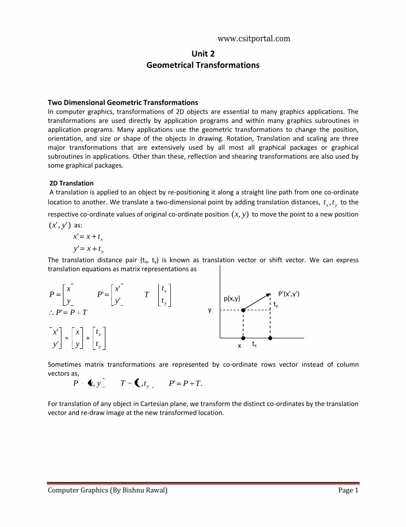
Two Dimensional Geometric Transformations In computer graphics, transformations of 2D objects are essential to many graphics applications. The transformations are used directly by application programs and within many graphics subroutines in application programs. Many applications use the geometric transformations to change the position, orientation, and size or shape of the objects in drawing. Rotation, Translation and scaling are three major transformations that are extensively used by all most all graphical packages or graphical subroutines in applications. Other than these, reflection and shearing transformations are also used by some graphical packages. 2D Translation A translation is applied to an object by re-positioning it along a straight line path from one co-ordinate
location to another. We translate a two-dimensional point by adding translation distances, yx tt , to the
respective co-ordinate values of original co-ordinate position ),( yx to move the point to a new position
)','( yx as:
xtxx'
ytxy'
The translation distance pair (tx, ty) is known as translation vector or shift vector. We can express translation equations as matrix representations as
y
xP
'
''
y
xP
y
x
t
tT
TPP'
'
'
y
x =
y
x +
y
x
t
t
Sometimes matrix transformations are represented by co-ordinate rows vector instead of column vectors as,
yxP , yx ttT , .' TPP
For translation of any object in Cartesian plane, we transform the distinct co-ordinates by the translation vector and re-draw image at the new transformed location.
p(x,y) ty
y
tx
P'(x',y')
x
www.csitportal.com
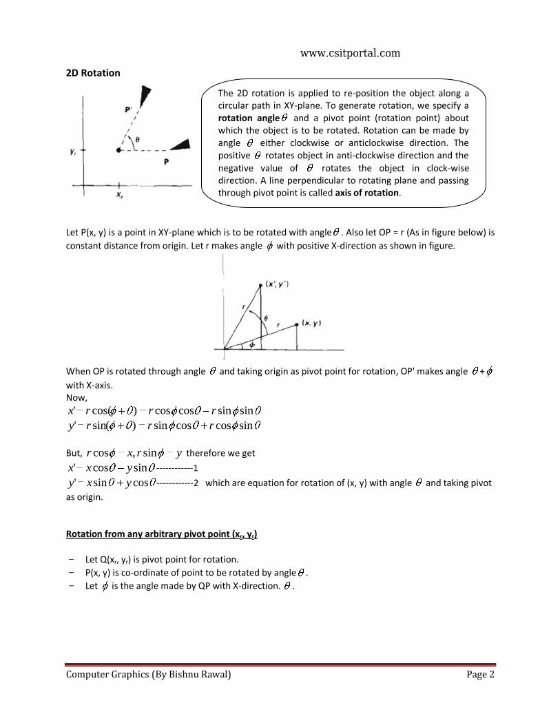
Computer Graphics (By Bishnu Rawal) Page 2
2D Rotation
Let P(x, y) is a point in XY-plane which is to be rotated with angle . Also let OP = r (As in figure below) is
constant distance from origin. Let r makes angle with positive X-direction as shown in figure.
When OP is rotated through angle and taking origin as pivot point for rotation, OP' makes angle +
with X-axis. Now,
sinsincoscos)cos(' rrrx
sincoscossin)sin(' rrry
But, yrxr sin,cos therefore we get
sincos' yxx ------------1
cossin' yxy ------------2 which are equation for rotation of (x, y) with angle and taking pivot
as origin. Rotation from any arbitrary pivot point (xr, yr)
− Let Q(xr, yr) is pivot point for rotation.
− P(x, y) is co-ordinate of point to be rotated by angle .
− Let is the angle made by QP with X-direction. .
The 2D rotation is applied to re-position the object along a circular path in XY-plane. To generate rotation, we specify a rotation angle and a pivot point (rotation point) about which the object is to be rotated. Rotation can be made by angle either clockwise or anticlockwise direction. The positive rotates object in anti-clockwise direction and the
negative value of rotates the object in clock-wise direction. A line perpendicular to rotating plane and passing through pivot point is called axis of rotation.
www.csitportal.com
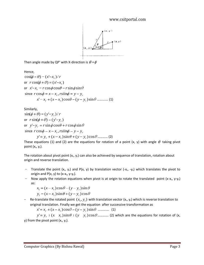
Computer Graphics (By Bishnu Rawal) Page 3
Then angle made by QP' with X-direction is +
Hence,
rxx r /)'()cos( or )'()cos( rxxr
or sinsincoscos' rrxx r
since rr yyrsiinxxr ,cos
sin)(cos)(' rrr yyxxxx …………. (1)
Similarly,
ryy r /)'()sin(
or )'()sin( ryyr
or sincoscossin' rryy r
since rr yyrsiinxxr ,cos
cos)(sin)(' rrr yyxxyy ………… (2)
These equations (1) and (2) are the equations for rotation of a point (x, y) with angle taking pivot point (xr, yr). The rotation about pivot point (xr, yr) can also be achieved by sequence of translation, rotation about origin and reverse translation.
− Translate the point (xr, yr) and P(x, y) by translation vector (-xr, -yr) which translates the pivot to origin and P(x, y) to (x-xr, y-yr).
− Now apply the rotation equations when pivot is at origin to rotate the translated point (x-xr, y-yr) as:
sin)(cos)(1 rr yyxxx
cos)(sin)(1 rr yyxxy
− Re-translate the rotated point ),( 11 yx with translation vector (xr, yr) which is reverse translation to
original translation. Finally we get the equation after successive transformation as
sin)(cos)(' rrr yyxxxx …………. (1)
cos)(sin)(' rrr yyxxyy …………. (2) which are the equations for rotation of (x,
y) from the pivot point (xr, yr).
www.csitportal.com
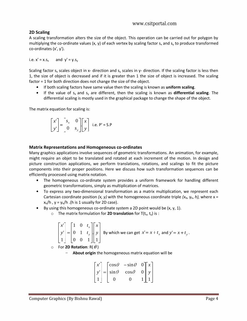
Computer Graphics (By Bishnu Rawal) Page 4
2D Scaling A scaling transformation alters the size of the object. This operation can be carried out for polygon by multiplying the co-ordinate values (x, y) of each vertex by scaling factor sx and sy to produce transformed co-ordinates (x', y'). i.e. x' = x.sx and y' = y.sy
Scaling factor sx scales object in x- direction and sy scales in y- direction. If the scaling factor is less then 1, the size of object is decreased and if it is greater than 1 the size of object is increased. The scaling factor = 1 for both direction does not change the size of the object.
If both scaling factors have same value then the scaling is known as uniform scaling.
If the value of sx and sy are different, then the scaling is known as differential scaling. The differential scaling is mostly used in the graphical package to change the shape of the object.
The matrix equation for scaling is:
y
x
s
s
y
x
y
x.
0
0
'
' i.e. P' = S.P
Matrix Representations and Homogeneous co-ordinates Many graphics applications involve sequences of geometric transformations. An animation, for example, might require an objet to be translated and rotated at each increment of the motion. In design and picture construction applications, we perform translations, rotations, and scalings to fit the picture components into their proper positions. Here we discuss how such transformation sequences can be efficiently processed using matrix notation.
The homogeneous co-ordinate system provides a uniform framework for handling different geometric transformations, simply as multiplication of matrices.
To express any two-dimensional transformation as a matrix multiplication, we represent each Cartesian coordinate position (x, y) with the homogeneous coordinate triple (xh, yh, h), where x = xh/h , y = yh/h .(h is 1 usually for 2D case).
By using this homogeneous co-ordinate system a 2D point would be (x, y, 1). o The matrix formulation for 2D translation for T(tx, ty) is :
1
.
100
10
01
1
'
'
y
x
t
t
y
x
y
x
By which we can get xtxx' and ytxy' .
o For 2D Rotation: R( )
− About origin the homogeneous matrix equation will be
1100
0cossin
0sincos
1
'
'
y
x
y
x
www.csitportal.com
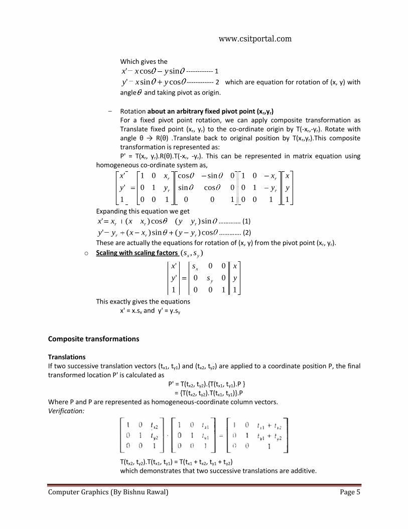
Computer Graphics (By Bishnu Rawal) Page 5
Which gives the
sincos' yxx ------------ 1
cossin' yxy ------------ 2 which are equation for rotation of (x, y) with
angle and taking pivot as origin.
− Rotation about an arbitrary fixed pivot point (xr,yr) For a fixed pivot point rotation, we can apply composite transformation as Translate fixed point (xr, yr) to the co-ordinate origin by T(-xr,-yr). Rotate with angle θ → R(θ) .Translate back to original position by T(xr,yr).This composite transformation is represented as: P' = T(xr, yr).R(θ).T(-xr, -yr). This can be represented in matrix equation using
homogeneous co-ordinate system as,
1100
10
01
100
0cossin
0sincos
100
10
01
1
'
'
y
x
y
x
y
x
y
x
r
r
r
r
Expanding this equation we get
sin)(cos)(' rrr yyxxxx …………. (1)
cos)(sin)(' rrr yyxxyy …………. (2)
These are actually the equations for rotation of (x, y) from the pivot point (xr, yr).
o Scaling with scaling factors ),( yx ss
1100
00
00
1
'
'
y
x
s
s
y
x
y
x
This exactly gives the equations
x' = x.sx and y' = y.sy
Composite transformations Translations If two successive translation vectors (tx1, ty1) and (tx2, ty2) are applied to a coordinate position P, the final transformed location P' is calculated as P' = T(tx2, ty2).{T(tx1, ty1).P } = {T(tx2, ty2).T(tx1, ty1)}.P Where P and P are represented as homogeneous-coordinate column vectors. Verification:
T(tx2, ty2).T(tx1, ty1) = T(tx1 + tx2, ty1 + ty2) which demonstrates that two successive translations are additive.
www.csitportal.com
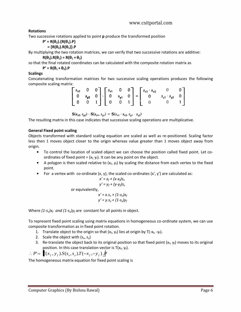
Computer Graphics (By Bishnu Rawal) Page 6
Rotations Two successive rotations applied to point p produce the transformed position
P’ = R(θ2).{R(θ1).P} = {R(θ2).R(θ1)}.P
By multiplying the two rotation matrices, we can verify that two successive rotations are additive: R(θ2).R(θ1) = R(θ1 + θ2)
so that the final rotated coordinates can be calculated with the composite rotation matrix as P’ = R(θ1 + θ2).P Scalings Concatenating transformation matrices for two successive scaling operations produces the following composite scaling matrix:
The resulting matrix in this case indicates that successive scaling operations are multiplicative. General Fixed point scaling Objects transformed with standard scaling equation are scaled as well as re-positioned. Scaling factor less then 1 moves object closer to the origin whereas value greater than 1 moves object away from origin.
To control the location of scaled object we can choose the position called fixed point. Let co-ordinates of fixed point = (xf, yf). It can be any point on the object.
A polygon is then scaled relative to (xf, yf) by scaling the distance from each vertex to the fixed point.
For a vertex with co-ordinate (x, y), the scaled co-ordinates (x', y') are calculated as:
x' = xf + (x-xf)sx
y' = yf + (y-yf)sy
or equivalently, x' = x.sx + (1-sx)xf
y' = y.sy + (1-sy)yf
Where (1-sx)xf and (1-sy)yf are constant for all points in object. To represent fixed point scaling using matrix equations in homogeneous co-ordinate system, we can use composite transformation as in fixed point rotation.
1. Translate object to the origin so that (xf, yf) lies at origin by T(-xf, -yf). 2. Scale the object with (sx, sy) 3. Re-translate the object back to its original position so that fixed point (xf, yf) moves to its original
position. In this case translation vector is T(xf, yf).
PyxTssSyxTP ffyxff .),().,().,('
The homogeneous matrix equation for fixed point scaling is
www.csitportal.com
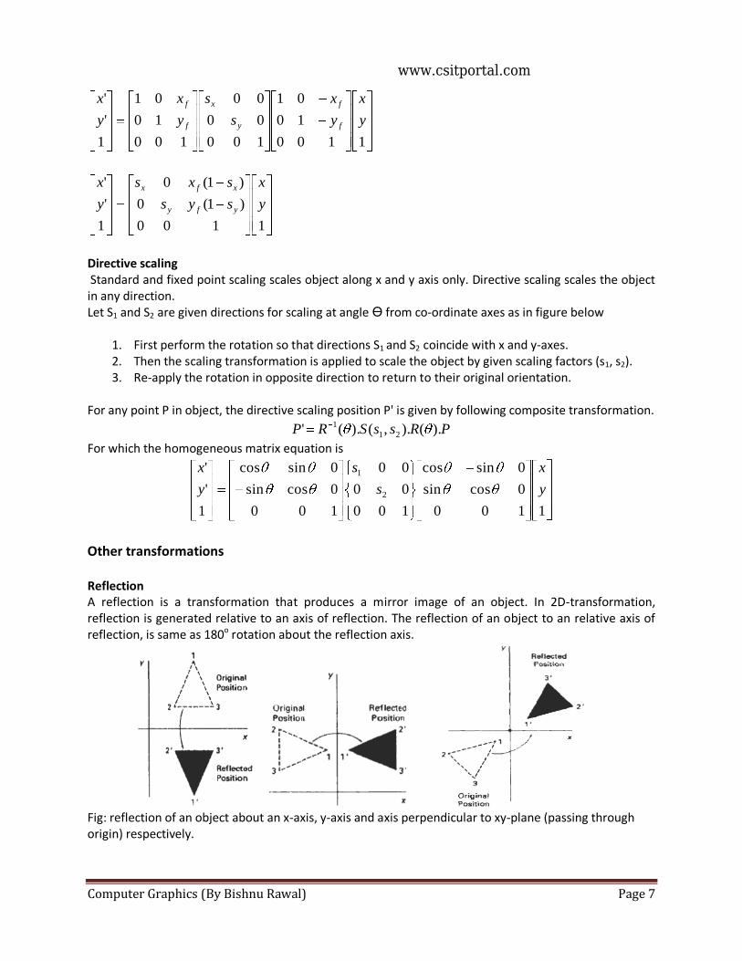
Computer Graphics (By Bishnu Rawal) Page 7
1100
10
01
100
00
00
100
10
01
1
'
'
y
x
y
x
s
s
y
x
y
x
f
f
y
x
f
f
1100
)1(0
)1(0
1
'
'
y
x
sys
sxs
y
x
yfy
xfx
Directive scaling Standard and fixed point scaling scales object along x and y axis only. Directive scaling scales the object in any direction. Let S1 and S2 are given directions for scaling at angle Ө from co-ordinate axes as in figure below
1. First perform the rotation so that directions S1 and S2 coincide with x and y-axes. 2. Then the scaling transformation is applied to scale the object by given scaling factors (s1, s2). 3. Re-apply the rotation in opposite direction to return to their original orientation.
For any point P in object, the directive scaling position P' is given by following composite transformation.
PRssSRP ).().,().(' 21
1
For which the homogeneous matrix equation is
1100
0cossin
0sincos
100
00
00
100
0cossin
0sincos
1
'
'
2
1
y
x
s
s
y
x
Other transformations Reflection A reflection is a transformation that produces a mirror image of an object. In 2D-transformation, reflection is generated relative to an axis of reflection. The reflection of an object to an relative axis of reflection, is same as 180o rotation about the reflection axis.
Fig: reflection of an object about an x-axis, y-axis and axis perpendicular to xy-plane (passing through origin) respectively.
www.csitportal.com
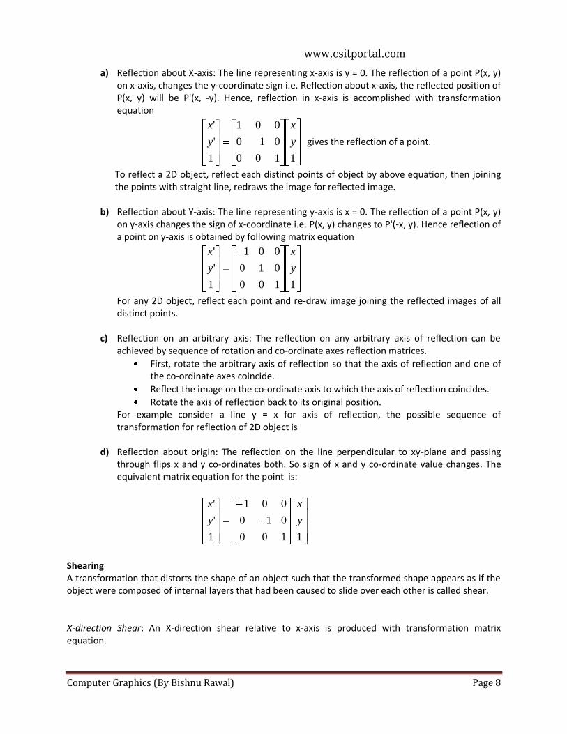
Computer Graphics (By Bishnu Rawal) Page 8
a) Reflection about X-axis: The line representing x-axis is y = 0. The reflection of a point P(x, y) on x-axis, changes the y-coordinate sign i.e. Reflection about x-axis, the reflected position of P(x, y) will be P'(x, -y). Hence, reflection in x-axis is accomplished with transformation equation
1100
010
001
1
'
'
y
x
y
x
gives the reflection of a point.
To reflect a 2D object, reflect each distinct points of object by above equation, then joining the points with straight line, redraws the image for reflected image.
b) Reflection about Y-axis: The line representing y-axis is x = 0. The reflection of a point P(x, y)
on y-axis changes the sign of x-coordinate i.e. P(x, y) changes to P'(-x, y). Hence reflection of a point on y-axis is obtained by following matrix equation
1100
010
001
1
'
'
y
x
y
x
For any 2D object, reflect each point and re-draw image joining the reflected images of all distinct points.
c) Reflection on an arbitrary axis: The reflection on any arbitrary axis of reflection can be achieved by sequence of rotation and co-ordinate axes reflection matrices.
First, rotate the arbitrary axis of reflection so that the axis of reflection and one of the co-ordinate axes coincide.
Reflect the image on the co-ordinate axis to which the axis of reflection coincides.
Rotate the axis of reflection back to its original position. For example consider a line y = x for axis of reflection, the possible sequence of transformation for reflection of 2D object is
d) Reflection about origin: The reflection on the line perpendicular to xy-plane and passing
through flips x and y co-ordinates both. So sign of x and y co-ordinate value changes. The equivalent matrix equation for the point is:
1100
010
001
1
'
'
y
x
y
x
Shearing A transformation that distorts the shape of an object such that the transformed shape appears as if the object were composed of internal layers that had been caused to slide over each other is called shear.
X-direction Shear: An X-direction shear relative to x-axis is produced with transformation matrix equation.
www.csitportal.com
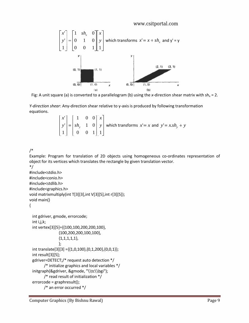
Computer Graphics (By Bishnu Rawal) Page 9
1100
010
01
1
'
'
y
xsh
y
x x
which transforms xshxx' and y' = y
Fig: A unit square (a) is converted to a parallelogram (b) using the x-direction shear matrix with shx = 2.
Y-direction shear: Any-direction shear relative to y-axis is produced by following transformation equations.
1100
01
001
1
'
'
y
x
shy
x
y which transforms xx' and yshxy y.'
/* Example: Program for translation of 2D objects using homogeneous co-ordinates representation of object for its vertices which translates the rectangle by given translation vector. */ #include<stdio.h> #include<conio.h> #include<stdlib.h> #include<graphics.h> void matrixmultiply(int T[3][3],int V[3][5],int r[3][5]); void main() { int gdriver, gmode, errorcode; int i,j,k; int vertex[3][5]={{100,100,200,200,100}, {100,200,200,100,100}, {1,1,1,1,1}, }; int translate[3][3] ={{1,0,100},{0,1,200},{0,0,1}}; int result[3][5]; gdriver=DETECT;/* request auto detection */ /* initialize graphics and local variables */ initgraph(&gdriver, &gmode, "\\tc\\bgi"); /* read result of initialization */ errorcode = graphresult(); /* an error occurred */
www.csitportal.com
Computer Graphics (By Bishnu Rawal) Page 10
if (errorcode != grOk) { printf("Graphics error: %s\n", grapherrormsg(errorcode)); printf("Press any key ...."); getch(); /* terminate with an error code */ } setbkcolor(2); for(i=0;i<4;i++) { setcolor(BLUE); line(vertex[0][i],vertex[1][i],vertex[0][i+1],vertex[1][i+1]); } printf("Press any key for the translated line.....\n"); getch(); matrixmultiply(translate,vertex,result); for(i=0;i<4;i++) { setcolor(YELLOW); line(result[0][i],result[1][i],result[0][i+1],result[1][i+1]); } getch(); closegraph(); } void matrixmultiply(int translate[3][3],int vertex[3][5],int result[3][5]) { for(int i=0;i<=3;i++) { for(int j=0;j<=5;j++) { result[i][j]=0; for(int k=0;k<=3;k++) result[i][j]+=translate[i][k]*vertex[k][j]; } } }
www.csitportal.com
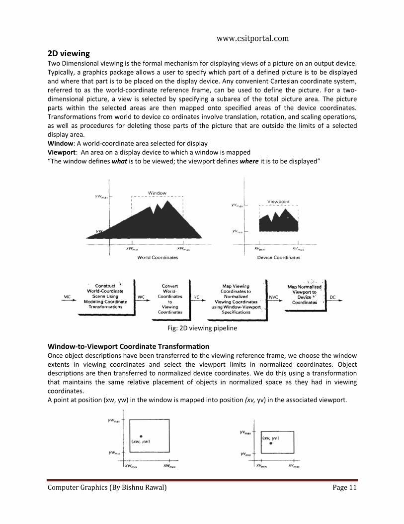
Computer Graphics (By Bishnu Rawal) Page 11
2D viewing Two Dimensional viewing is the formal mechanism for displaying views of a picture on an output device. Typically, a graphics package allows a user to specify which part of a defined picture is to be displayed and where that part is to be placed on the display device. Any convenient Cartesian coordinate system, referred to as the world-coordinate reference frame, can be used to define the picture. For a two-dimensional picture, a view is selected by specifying a subarea of the total picture area. The picture parts within the selected areas are then mapped onto specified areas of the device coordinates. Transformations from world to device co ordinates involve translation, rotation, and scaling operations, as well as procedures for deleting those parts of the picture that are outside the limits of a selected display area. Window: A world-coordinate area selected for display Viewport: An area on a display device to which a window is mapped “The window defines what is to be viewed; the viewport defines where it is to be displayed”
Fig: 2D viewing pipeline
Window-to-Viewport Coordinate Transformation Once object descriptions have been transferred to the viewing reference frame, we choose the window extents in viewing coordinates and select the viewport limits in normalized coordinates. Object descriptions are then transferred to normalized device coordinates. We do this using a transformation that maintains the same relative placement of objects in normalized space as they had in viewing coordinates. A point at position (xw, yw) in the window is mapped into position (xv, yv) in the associated viewport.
www.csitportal.com
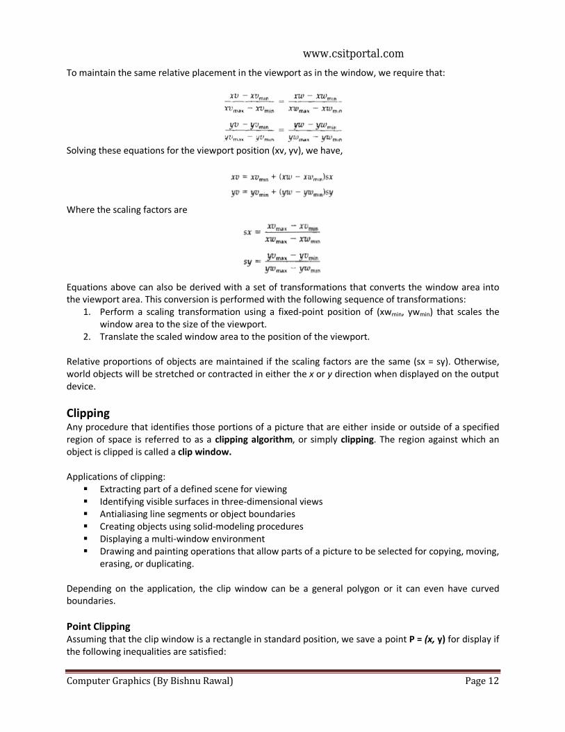
Computer Graphics (By Bishnu Rawal) Page 12
To maintain the same relative placement in the viewport as in the window, we require that:
Solving these equations for the viewport position (xv, yv), we have,
Where the scaling factors are
Equations above can also be derived with a set of transformations that converts the window area into the viewport area. This conversion is performed with the following sequence of transformations:
1. Perform a scaling transformation using a fixed-point position of (xwmin, ywmin) that scales the window area to the size of the viewport.
2. Translate the scaled window area to the position of the viewport.
Relative proportions of objects are maintained if the scaling factors are the same (sx = sy). Otherwise, world objects will be stretched or contracted in either the x or y direction when displayed on the output device.
Clipping Any procedure that identifies those portions of a picture that are either inside or outside of a specified region of space is referred to as a clipping algorithm, or simply clipping. The region against which an object is clipped is called a clip window. Applications of clipping:
Extracting part of a defined scene for viewing Identifying visible surfaces in three-dimensional views Antialiasing line segments or object boundaries Creating objects using solid-modeling procedures Displaying a multi-window environment Drawing and painting operations that allow parts of a picture to be selected for copying, moving,
erasing, or duplicating. Depending on the application, the clip window can be a general polygon or it can even have curved boundaries.
Point Clipping Assuming that the clip window is a rectangle in standard position, we save a point P = (x, y) for display if the following inequalities are satisfied:
www.csitportal.com
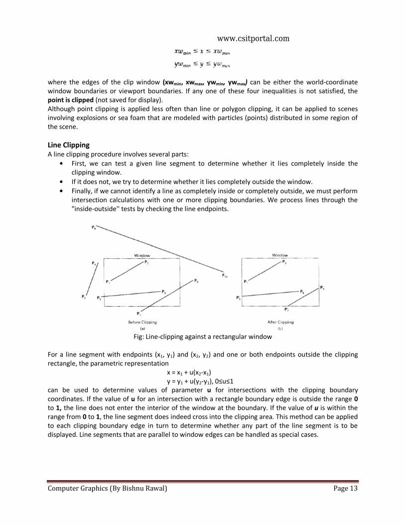
Computer Graphics (By Bishnu Rawal) Page 13
where the edges of the clip window (xwmin, xwmax, ywmin, ywmax) can be either the world-coordinate window boundaries or viewport boundaries. If any one of these four inequalities is not satisfied, the point is clipped (not saved for display). Although point clipping is applied less often than line or polygon clipping, it can be applied to scenes involving explosions or sea foam that are modeled with particles (points) distributed in some region of the scene.
Line Clipping A line clipping procedure involves several parts:
First, we can test a given line segment to determine whether it lies completely inside the clipping window.
If it does not, we try to determine whether it lies completely outside the window.
Finally, if we cannot identify a line as completely inside or completely outside, we must perform intersection calculations with one or more clipping boundaries. We process lines through the "inside-outside'' tests by checking the line endpoints.
Fig: Line-clipping against a rectangular window
For a line segment with endpoints (x1, y1) and (x2, y2) and one or both endpoints outside the clipping rectangle, the parametric representation
x = x1 + u(x2-x1) y = y1 + u(y2-y1), 0≤u≤1
can be used to determine values of parameter u for intersections with the clipping boundary coordinates. If the value of u for an intersection with a rectangle boundary edge is outside the range 0 to 1, the line does not enter the interior of the window at the boundary. If the value of u is within the range from 0 to 1, the line segment does indeed cross into the clipping area. This method can be applied to each clipping boundary edge in turn to determine whether any part of the line segment is to be displayed. Line segments that are parallel to window edges can be handled as special cases.
www.csitportal.com
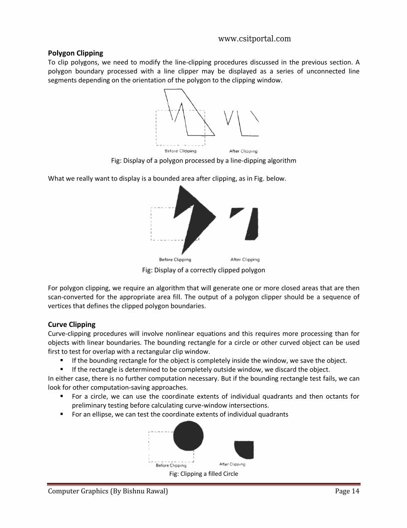
Computer Graphics (By Bishnu Rawal) Page 14
Polygon Clipping To clip polygons, we need to modify the line-clipping procedures discussed in the previous section. A polygon boundary processed with a line clipper may be displayed as a series of unconnected line segments depending on the orientation of the polygon to the clipping window.
Fig: Display of a polygon processed by a line-dipping algorithm
What we really want to display is a bounded area after clipping, as in Fig. below.
Fig: Display of a correctly clipped polygon
For polygon clipping, we require an algorithm that will generate one or more closed areas that are then scan-converted for the appropriate area fill. The output of a polygon clipper should be a sequence of vertices that defines the clipped polygon boundaries.
Curve Clipping Curve-clipping procedures will involve nonlinear equations and this requires more processing than for objects with linear boundaries. The bounding rectangle for a circle or other curved object can be used first to test for overlap with a rectangular clip window.
If the bounding rectangle for the object is completely inside the window, we save the object. If the rectangle is determined to be completely outside window, we discard the object.
In either case, there is no further computation necessary. But if the bounding rectangle test fails, we can look for other computation-saving approaches.
For a circle, we can use the coordinate extents of individual quadrants and then octants for preliminary testing before calculating curve-window intersections.
For an ellipse, we can test the coordinate extents of individual quadrants
Fig: Clipping a filled Circle
www.csitportal.com
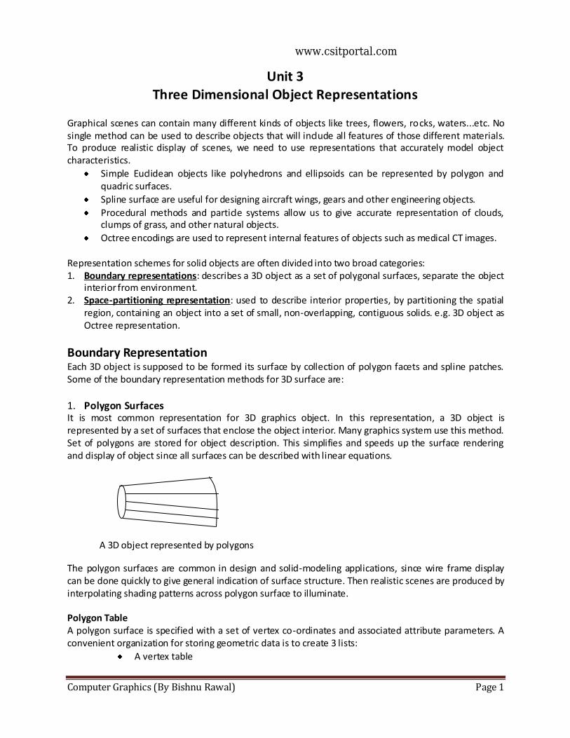
Computer Graphics (By Bishnu Rawal) Page 1
Unit 3 Three Dimensional Object Representations
Graphical scenes can contain many different kinds of objects like trees, flowers, rocks, waters...etc. No single method can be used to describe objects that will include all features of those different materials. To produce realistic display of scenes, we need to use representations that accurately model object characteristics.
Simple Euclidean objects like polyhedrons and ellipsoids can be represented by polygon and quadric surfaces.
Spline surface are useful for designing aircraft wings, gears and other engineering objects.
Procedural methods and particle systems allow us to give accurate representation of clouds, clumps of grass, and other natural objects.
Octree encodings are used to represent internal features of objects such as medical CT images. Representation schemes for solid objects are often divided into two broad categories: 1. Boundary representations: describes a 3D object as a set of polygonal surfaces, separate the object
interior from environment. 2. Space-partitioning representation: used to describe interior properties, by partitioning the spatial
region, containing an object into a set of small, non-overlapping, contiguous solids. e.g. 3D object as Octree representation.
Boundary Representation
Each 3D object is supposed to be formed its surface by collection of polygon facets and spline patches. Some of the boundary representation methods for 3D surface are:
1. Polygon Surfaces It is most common representation for 3D graphics object. In this representation, a 3D object is represented by a set of surfaces that enclose the object interior. Many graphics system use this method. Set of polygons are stored for object description. This simplifies and speeds up the surface rendering and display of object since all surfaces can be described with linear equations. The polygon surfaces are common in design and solid-modeling applications, since wire frame display can be done quickly to give general indication of surface structure. Then realistic scenes are produced by interpolating shading patterns across polygon surface to illuminate. Polygon Table A polygon surface is specified with a set of vertex co-ordinates and associated attribute parameters. A convenient organization for storing geometric data is to create 3 lists:
A vertex table
A 3D object represented by polygons
www.csitportal.com
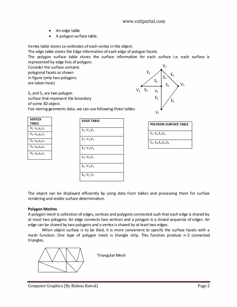
Computer Graphics (By Bishnu Rawal) Page 2
An edge table
A polygon surface table. Vertex table stores co-ordinates of each vertex in the object. The edge table stores the Edge information of each edge of polygon facets. The polygon surface table stores the surface information for each surface i.e. each surface is represented by edge lists of polygon. Consider the surface contains polygonal facets as shown in figure (only two polygons are taken here) S1 and S2 are two polygon surface that represent the boundary of some 3D object. Foe storing geometric data, we can use following three tables
VERTEX TABLE
V1: x1,y1,z1
V2: x2,y2,z2
V3: x3,y3,z3
V4: x4,y4,z4
V5: x5,y5,z5
The object can be displayed efficiently by using data from tables and processing them for surface rendering and visible surface determination. Polygon Meshes A polygon mesh is collection of edges, vertices and polygons connected such that each edge is shared by at most two polygons. An edge connects two vertices and a polygon is a closed sequence of edges. An edge can be shared by two polygons and a vertex is shared by at least two edges. When object surface is to be tiled, it is more convenient to specify the surface facets with a mesh function. One type of polygon mesh is triangle strip. This function produce n-2 connected triangles.
V1
E6
V5
E5 S1
S2
E1
V2 E2 V3
3 E3
V4
4
E4
EDGE TABLE
E1: V1,V2
E2: V2,V3
E3: V3,V4
E4: V4,V5
E5: V1,V3
E6: V5, V1
POLYGON SURFACE TABLE
S1: E1,E2,E3
S2: E3,E4,E5,E6
Triangular Mesh
www.csitportal.com
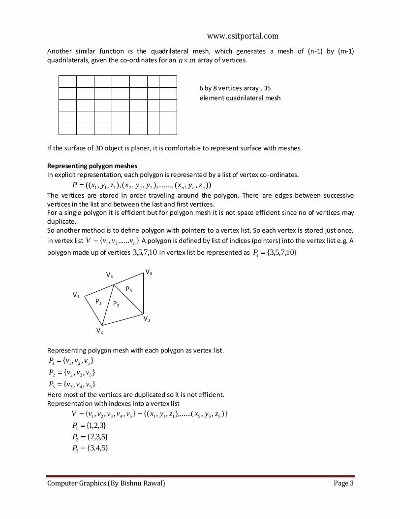
Computer Graphics (By Bishnu Rawal) Page 3
Another similar function is the quadrilateral mesh, which generates a mesh of (n-1) by (m-1) quadrilaterals, given the co-ordinates for an mn array of vertices. If the surface of 3D object is planer, it is comfortable to represent surface with meshes. Representing polygon meshes In explicit representation, each polygon is represented by a list of vertex co-ordinates.
)),,(),.......,,,(),,,(( 222111 nnn zyxyyxzyxP
The vertices are stored in order traveling around the polygon. There are edges between successive vertices in the list and between the last and first vertices. For a single polygon it is efficient but for polygon mesh it is not space efficient since no of vertices may duplicate. So another method is to define polygon with pointers to a vertex list. So each vertex is stored just once,
in vertex list }......,{ 21 nvvvV A polygon is defined by list of indices (pointers) into the vertex list e.g. A
polygon made up of vertices 10,7,5,3 in vertex list be represented as }10,7,5,3{1P
Representing polygon mesh with each polygon as vertex list.
},,{ 5211 vvvP
},,{ 5322 vvvP
},,{ 5433 vvvP
Here most of the vertices are duplicated so it is not efficient. Representation with indexes into a vertex list
)},,),......(,,{(},,,,{ 55511154321 zyxzyxvvvvvV
}3,2,1{1P
}5,3,2{2P
}5,4,3{3P
V2
V5
V1
P3
V3
V4
P1 P2
6 by 8 vertices array , 35
element quadrilateral mesh
www.csitportal.com
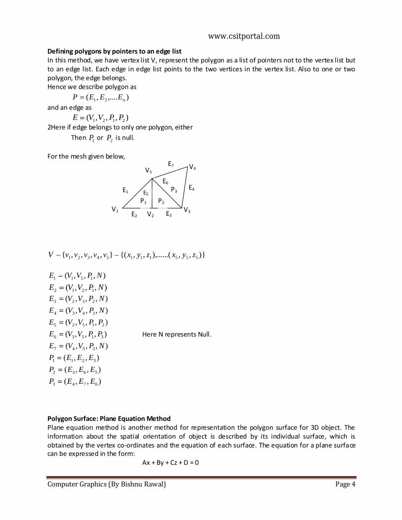
Computer Graphics (By Bishnu Rawal) Page 4
Defining polygons by pointers to an edge list In this method, we have vertex list V, represent the polygon as a list of pointers not to the vertex list but to an edge list. Each edge in edge list points to the two vertices in the vertex list. Also to one or two polygon, the edge belongs. Hence we describe polygon as
),....,( 21 nEEEP
and an edge as
),,,( 2121 PPVVE
2Here if edge belongs to only one polygon, either
Then 1P or
2P is null.
For the mesh given below,
)},,),......(,,{(},,,,{ 55511154321 zyxzyxvvvvvV
),,,( 1511 NPVVE
),,,( 1212 NPVVE
),,,( 2323 NPVVE
),,,( 3434 NPVVE
),,,( 21525 PPVVE
),,,( 31536 PPVVE Here N represents Null.
),,,( 3547 NPVVE
),,( 3211 EEEP
),,( 5632 EEEP
),,( 6743 EEEP
Polygon Surface: Plane Equation Method Plane equation method is another method for representation the polygon surface for 3D object. The information about the spatial orientation of object is described by its individual surface, which is obtained by the vertex co-ordinates and the equation of each surface. The equation for a plane surface can be expressed in the form: Ax + By + Cz + D = 0
V3 E3 V2 E2
V1
V4 E7
V5
E1
E6
P3
P2 P1
E5
E4
www.csitportal.com
Computer Graphics (By Bishnu Rawal) Page 5
Where (x, y, z) is any point on the plane, and A, B, C, D are constants describing the spatial properties of the plane. The values of A, B, C, D can be obtained by solving a set of three plane equations using co-ordinate values of 3 noncollinear points on the plane. Let (x1, y1, z1), (x2, y3, z2) and (x3, y3, z3) are three such points on the plane, then, Ax1 + By1 + Cz1 + D = 0 Ax2 + By2 + Cz2 + D = 0 Ax3 + By3 + Cz3 + D = 0 The solution of these equations can be obtained in determinant from using Cramer’s rule as:-
A =
33
22
11
1
1
1
zy
zy
zy
B =
33
22
11
1
1
1
zx
zx
zx
C =
1
1
1
31
21
11
yx
yx
yx
D =
331
221
111
zyx
zyx
zyx
For any points (x, y, z)
If Ax + By + Cz + D 0, then (x, y, z) is not on the plane. If Ax + By + Cz + D < 0, then (x, y, z) is inside the plane i. e. invisible side If Ax + By + Cz + D > 0, then (x, y, z) is lies out side the surface.
2. Quadric Surface Quadric Surface is one of the frequently used 3D objects surface representation. The quadric surface can be represented by a second degree polynomial. This includes:
1. Sphere: For the set of surface points (x, y, z) the spherical surface is represented as: x2+y2+z2 = r2, with radius r and centered at co-ordinate origin.
2. Ellipsoid: 12
2
2
2
2
2
c
z
b
y
a
x , where (x, y, z) is the surface points and a, b, c are the radii on X, Y
and Z directions respectively.
3. Elliptic parboiled: zb
y
a
x2
2
2
2
4. Hyperbolic parboiled : zb
y
a
x2
2
2
2
5. Elliptic cone : 02
2
2
2
2
2
c
z
b
y
a
x
6. Hyperboloid of one sheet: 12
2
2
2
2
2
c
z
b
y
a
x
7. Hyperboloid of two sheet: 12
2
2
2
2
2
c
z
b
y
a
x
3. Wireframe Representation: In this method 3D objects is represented as a list of straight lines, each of which is represented by its two end points (x1, y1, z1) and (x2, y2, z2). This method only shows the skeletal structure of the objects. It is simple and can see through the object and fast method. But independent line data structure is very inefficient i.e. don’t know what is connected to what. In this method the scenes represented are not realistic.
www.csitportal.com
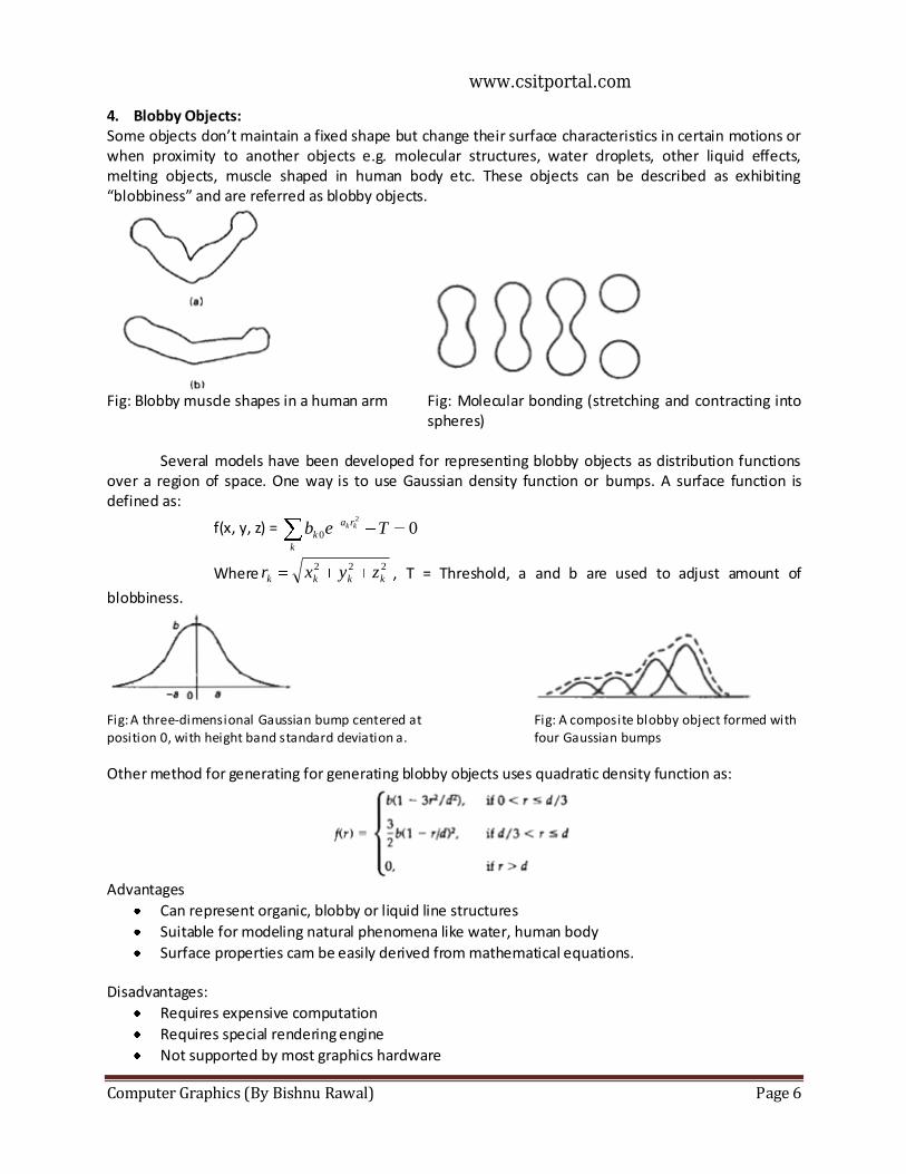
Computer Graphics (By Bishnu Rawal) Page 6
4. Blobby Objects: Some objects don’t maintain a fixed shape but change their surface characteristics in certain motions or when proximity to another objects e.g. molecular structures, water droplets, other liquid effects, melting objects, muscle shaped in human body etc. These objects can be described as exhibiting “blobbiness” and are referred as blobby objects.
Fig: Blobby muscle shapes in a human arm Fig: Molecular bonding (stretching and contracting into
spheres) Several models have been developed for representing blobby objects as distribution functions
over a region of space. One way is to use Gaussian density function or bumps. A surface function is defined as:
f(x, y, z) = 02
0 Teb kkra
k
k
Where222
kkkk zyxr , T = Threshold, a and b are used to adjust amount of
blobbiness.
Fig: A three-dimensional Gaussian bump centered at Fig: A composite blobby object formed with position 0, with height band standard deviation a. four Gaussian bumps
Other method for generating for generating blobby objects uses quadratic density function as:
Advantages
Can represent organic, blobby or liquid line structures
Suitable for modeling natural phenomena like water, human body
Surface properties cam be easily derived from mathematical equations. Disadvantages:
Requires expensive computation
Requires special rendering engine
Not supported by most graphics hardware
www.csitportal.com
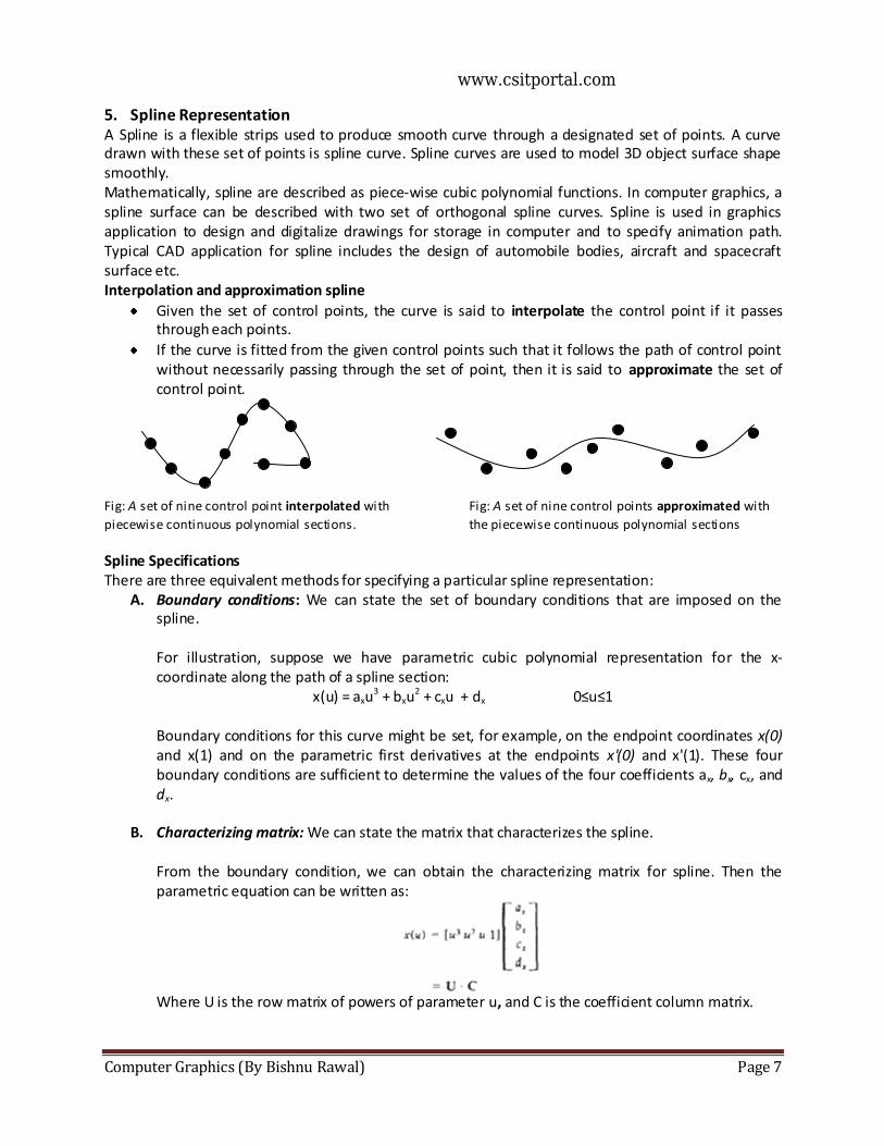
Computer Graphics (By Bishnu Rawal) Page 7
5. Spline Representation A Spline is a flexible strips used to produce smooth curve through a designated set of points. A curve drawn with these set of points is spline curve. Spline curves are used to model 3D object surface shape smoothly. Mathematically, spline are described as piece-wise cubic polynomial functions. In computer graphics, a spline surface can be described with two set of orthogonal spline curves. Spline is used in graphics application to design and digitalize drawings for storage in computer and to specify animation path. Typical CAD application for spline includes the design of automobile bodies, aircraft and spacecraft surface etc. Interpolation and approximation spline
Given the set of control points, the curve is said to interpolate the control point if it passes through each points.
If the curve is fitted from the given control points such that it follows the path of control point without necessarily passing through the set of point, then it is said to approximate the set of control point.
Fig: A set of nine control point interpolated with Fig: A set of nine control points approximated with
piecewise continuous polynomial sections. the piecewise continuous polynomial sections Spline Specifications There are three equivalent methods for specifying a particular spline representation:
A. Boundary conditions: We can state the set of boundary conditions that are imposed on the spline. For illustration, suppose we have parametric cubic polynomial representation for the x-coordinate along the path of a spline section:
x(u) = axu3 + bxu
2 + cxu + dx 0≤u≤1
Boundary conditions for this curve might be set, for example, on the endpoint coordinates x(0) and x(1) and on the parametric first derivatives at the endpoints x'(0) and x'(1). These four boundary conditions are sufficient to determine the values of the four coefficients ax, bx, cx, and dx.
B. Characterizing matrix: We can state the matrix that characterizes the spline. From the boundary condition, we can obtain the characterizing matrix for spline. Then the parametric equation can be written as:
Where U is the row matrix of powers of parameter u, and C is the coefficient column matrix.
www.csitportal.com
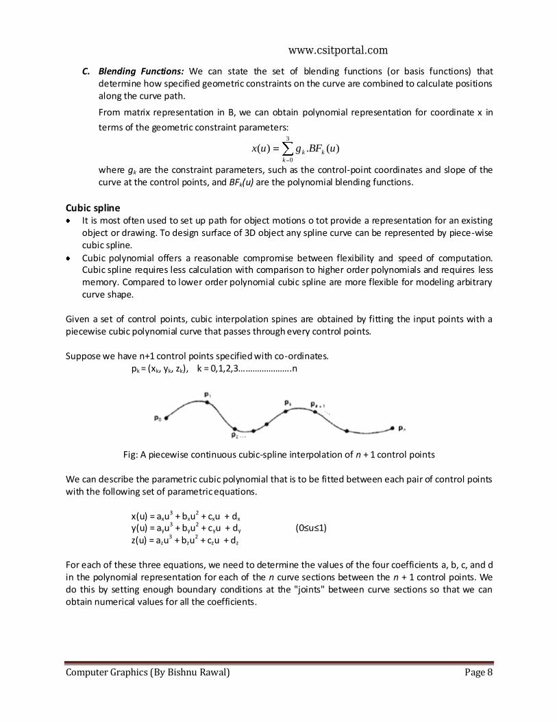
Computer Graphics (By Bishnu Rawal) Page 8
C. Blending Functions: We can state the set of blending functions (or basis functions) that determine how specified geometric constraints on the curve are combined to calculate positions along the curve path.
From matrix representation in B, we can obtain polynomial representation for coordinate x in
terms of the geometric constraint parameters: 3
0
)(.)(k
kk uBFgux
where gk are the constraint parameters, such as the control-point coordinates and slope of the curve at the control points, and BFk(u) are the polynomial blending functions.
Cubic spline It is most often used to set up path for object motions o tot provide a representation for an existing
object or drawing. To design surface of 3D object any spline curve can be represented by piece-wise cubic spline.
Cubic polynomial offers a reasonable compromise between flexibility and speed of computation. Cubic spline requires less calculation with comparison to higher order polynomials and requires less memory. Compared to lower order polynomial cubic spline are more flexible for modeling arbitrary curve shape.
Given a set of control points, cubic interpolation spines are obtained by fitting the input points with a piecewise cubic polynomial curve that passes through every control points. Suppose we have n+1 control points specified with co-ordinates. pk = (xk, yk, zk), k = 0,1,2,3…………………..n
Fig: A piecewise continuous cubic-spline interpolation of n + 1 control points
We can describe the parametric cubic polynomial that is to be fitted between each pair of control points with the following set of parametric equations. x(u) = axu
3 + bxu2 + cxu + dx
y(u) = ayu3 + byu
2 + cyu + dy (0≤u≤1)
z(u) = azu3 + bzu
2 + czu + dz
For each of these three equations, we need to determine the values of the four coefficients a, b, c, and d in the polynomial representation for each of the n curve sections between the n + 1 control points. We do this by setting enough boundary conditions at the "joints" between curve sections so that we can obtain numerical values for all the coefficients.
www.csitportal.com
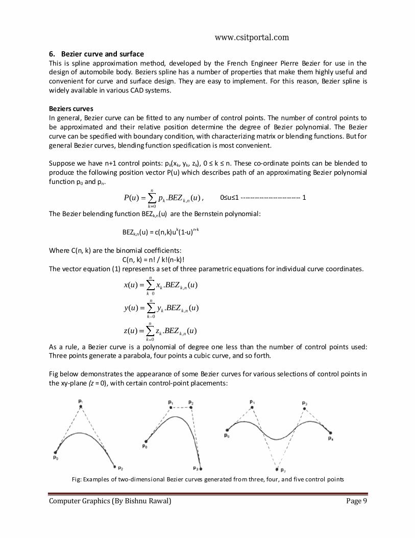
Computer Graphics (By Bishnu Rawal) Page 9
6. Bezier curve and surface This is spline approximation method, developed by the French Engineer Pierre Bezier for use in the design of automobile body. Beziers spline has a number of properties that make them highly useful and convenient for curve and surface design. They are easy to implement. For this reason, Bezier spline is widely available in various CAD systems. Beziers curves In general, Bezier curve can be fitted to any number of control points. The number of control points to be approximated and their relative position determine the degree of Bezier polynomial. The Bezier curve can be specified with boundary condition, with characterizing matrix or blending functions. But for general Bezier curves, blending function specification is most convenient. Suppose we have n+1 control points: pk(xk, yk, zk), 0 ≤ k ≤ n. These co-ordinate points can be blended to produce the following position vector P(u) which describes path of an approximating Bezier polynomial function p0 and pn.
n
k
nkk uBEZpuP0
, )(.)( , 0≤u≤1 -------------------------- 1
The Bezier belending function BEZk,n(u) are the Bernstein polynomial: BEZk,n(u) = c(n,k)uk(1-u)n-k
Where C(n, k) are the binomial coefficients: C(n, k) = n! / k!(n-k)! The vector equation (1) represents a set of three parametric equations for individual curve coordinates.
n
k
nkk uBEZxux0
, )(.)(
n
k
nkk uBEZyuy0
, )(.)(
n
k
nkk uBEZzuz0
, )(.)(
As a rule, a Bezier curve is a polynomial of degree one less than the number of control points used: Three points generate a parabola, four points a cubic curve, and so forth. Fig below demonstrates the appearance of some Bezier curves for various selections of control points in the xy-plane (z = 0), with certain control-point placements:
Fig: Examples of two-dimensional Bezier curves generated from three, four, and five control points
www.csitportal.com
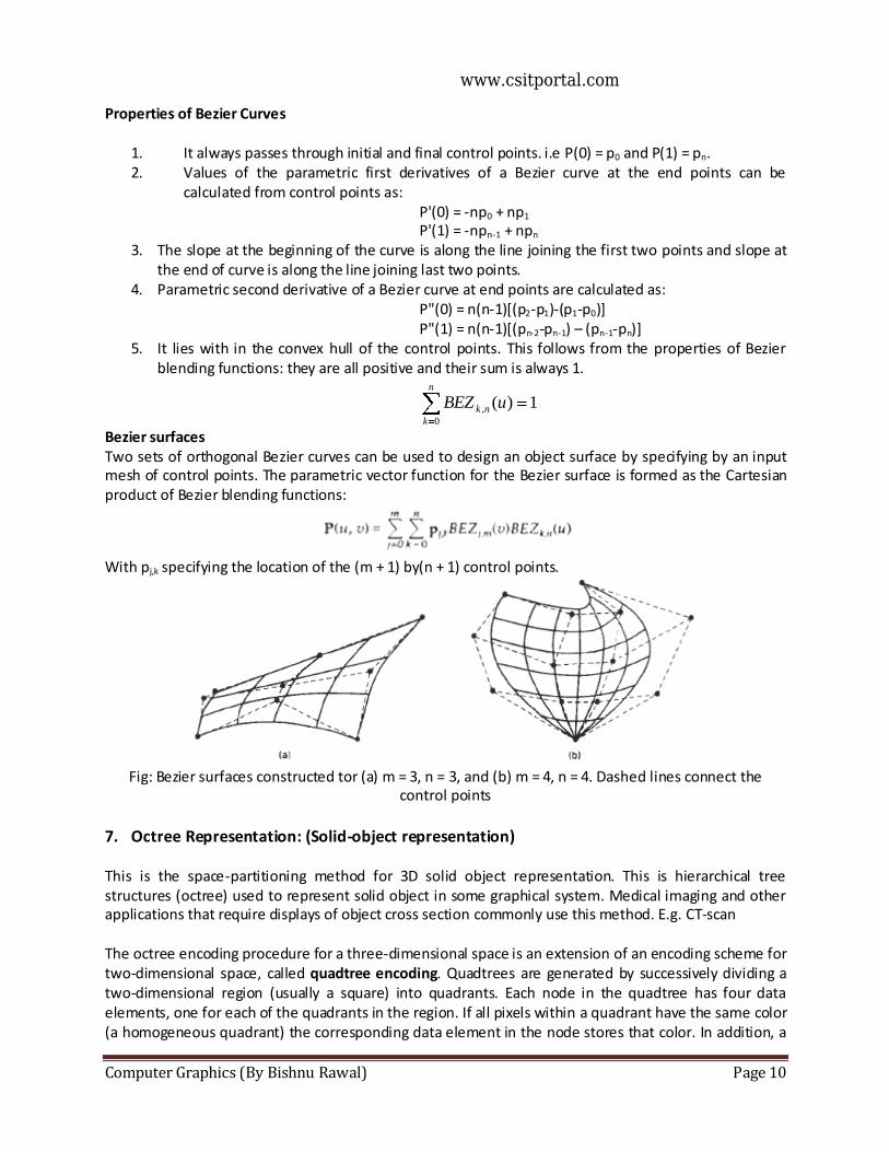
Computer Graphics (By Bishnu Rawal) Page 10
Properties of Bezier Curves
1. It always passes through initial and final control points. i.e P(0) = p0 and P(1) = pn. 2. Values of the parametric first derivatives of a Bezier curve at the end points can be
calculated from control points as: P'(0) = -np0 + np1 P'(1) = -npn-1 + npn
3. The slope at the beginning of the curve is along the line joining the first two points and slope at the end of curve is along the line joining last two points.
4. Parametric second derivative of a Bezier curve at end points are calculated as: P"(0) = n(n-1)[(p2-p1)-(p1-p0)]
P"(1) = n(n-1)[(pn-2-pn-1) – (pn-1-pn)] 5. It lies with in the convex hull of the control points. This follows from the properties of Bezier
blending functions: they are all positive and their sum is always 1.
1)(0
,
n
k
nk uBEZ
Bezier surfaces Two sets of orthogonal Bezier curves can be used to design an object surface by specifying by an input mesh of control points. The parametric vector function for the Bezier surface is formed as the Cartesian product of Bezier blending functions:
With pj,k specifying the location of the (m + 1) by(n + 1) control points.
Fig: Bezier surfaces constructed tor (a) m = 3, n = 3, and (b) m = 4, n = 4. Dashed lines connect the
control points
7. Octree Representation: (Solid-object representation) This is the space-partitioning method for 3D solid object representation. This is hierarchical tree structures (octree) used to represent solid object in some graphical system. Medical imaging and other applications that require displays of object cross section commonly use this method. E.g. CT-scan The octree encoding procedure for a three-dimensional space is an extension of an encoding scheme for two-dimensional space, called quadtree encoding. Quadtrees are generated by successively dividing a two-dimensional region (usually a square) into quadrants. Each node in the quadtree has four data elements, one for each of the quadrants in the region. If all pixels within a quadrant have the same color (a homogeneous quadrant) the corresponding data element in the node stores that color. In addition, a
www.csitportal.com
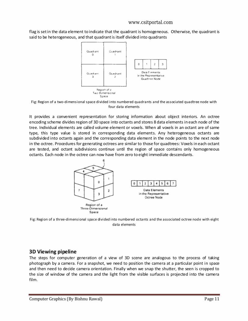
Computer Graphics (By Bishnu Rawal) Page 11
flag is set in the data element to indicate that the quadrant is homogeneous. Otherwise, the quadrant is said to be heterogeneous, and that quadrant is itself divided into quadrants
Fig: Region of a two-dimensional space divided into numbered quadrants and the associated quadtree node with
four data elements
It provides a convenient representation for storing information about object interiors. An octree encoding scheme divides region of 3D space into octants and stores 8 data elements in each node of the tree. Individual elements are called volume element or voxels. When all voxels in an octant are of same type, this type value is stored in corresponding data elements. Any heterogeneous octants are subdivided into octants again and the corresponding data element in the node points to the next node in the octree. Procedures for generating octrees are similar to those for quadtrees: Voxels in each octant are tested, and octant subdivisions continue until the region of space contains only homogeneous octants. Each node in the octree can now have from zero to eight immediate descendants.
Fig: Region of a three-dimensional space divided into numbered octants and the associated octree node with eight
data elements
3D Viewing pipeline The steps for computer generation of a view of 3D scene are analogous to the process of taking photograph by a camera. For a snapshot, we need to position the camera at a particular point in space and then need to decide camera orientation. Finally when we snap the shutter, the seen is cropped to the size of window of the camera and the light from the visible surfaces is projected into the camera film.
www.csitportal.com
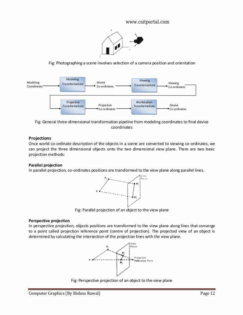
Computer Graphics (By Bishnu Rawal) Page 12
Fig: Photographing a scene involves selection of a camera position and orientation
Fig: General three-dimensional transformation pipeline from modeling coordinates to final device coordinates
Projections Once world co-ordinate description of the objects in a scene are converted to viewing co-ordinates, we can project the three dimensional objects onto the two dimensional view plane. There are two basic projection methods: Parallel projection In parallel projection, co-ordinates positions are transformed to the view plane along parallel lines.
Fig: Parallel projection of an object to the view plane
Perspective projection In perspective projection, objects positions are transformed to the view plane along lines that converge to a point called projection reference point (centre of projection). The projected view of an object is determined by calculating the intersection of the projection lines with the view plane.
Fig: Perspective projection of an object to the view plane
Modeling
Transformations Modeling Coordinates
World Co-ordinates
Viewing
Transformations Viewing Co-ordinates
Projection Transformations Projection
Co-ordinates
Workstation Transformations Device
Co-ordinates
www.csitportal.com
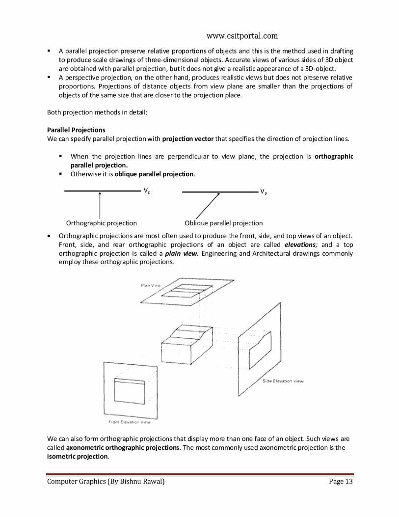
Computer Graphics (By Bishnu Rawal) Page 13
A parallel projection preserve relative proportions of objects and this is the method used in drafting to produce scale drawings of three-dimensional objects. Accurate views of various sides of 3D object are obtained with parallel projection, but it does not give a realistic appearance of a 3D-object.
A perspective projection, on the other hand, produces realistic views but does not preserve relative proportions. Projections of distance objects from view plane are smaller than the projections of objects of the same size that are closer to the projection place.
Both projection methods in detail: Parallel Projections We can specify parallel projection with projection vector that specifies the direction of projection lines.
When the projection lines are perpendicular to view plane, the projection is orthographic
parallel projection. Otherwise it is oblique parallel projection.
Orthographic projections are most often used to produce the front, side, and top views of an object. Front, side, and rear orthographic projections of an object are called elevations; and a top orthographic projection is called a plain view. Engineering and Architectural drawings commonly employ these orthographic projections.
We can also form orthographic projections that display more than one face of an object. Such views are called axonometric orthographic projections. The most commonly used axonometric projection is the isometric projection.
Vp Vp
Oblique parallel projection Orthographic projection
www.csitportal.com
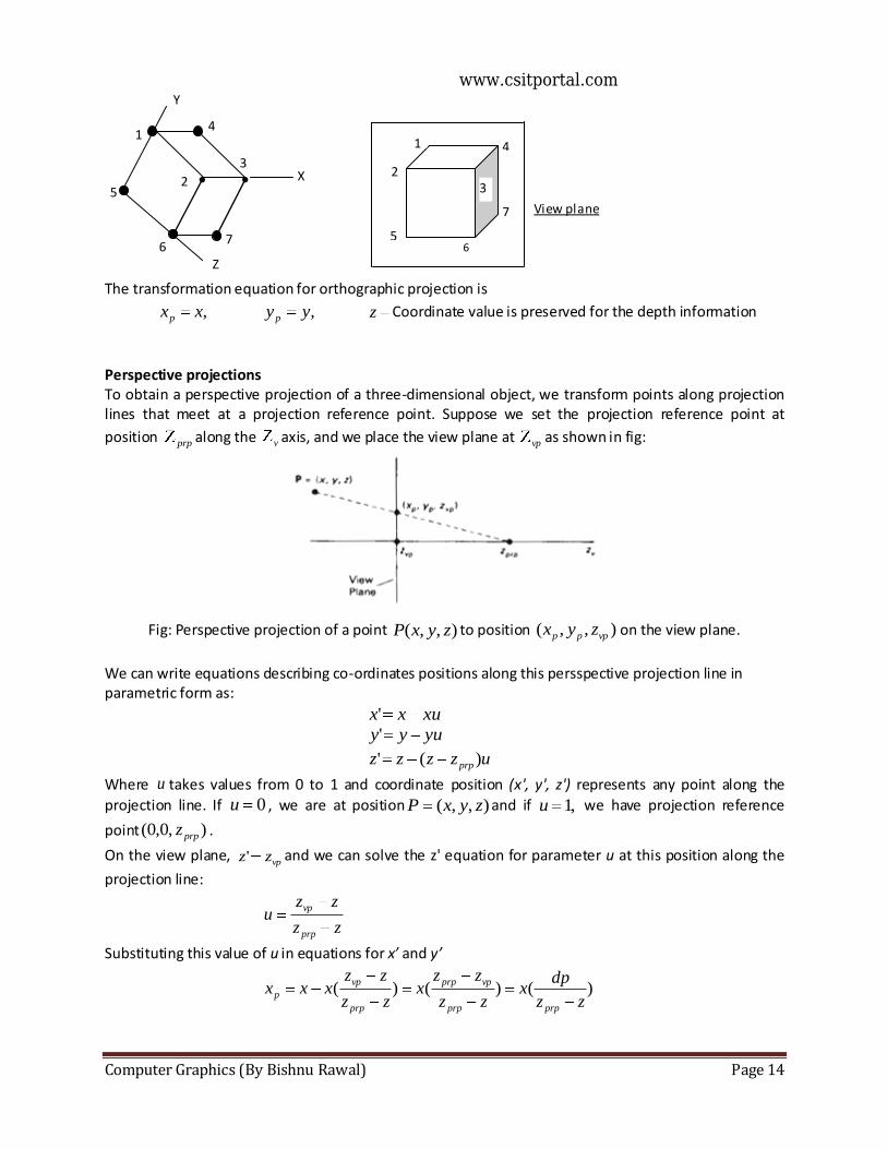
Computer Graphics (By Bishnu Rawal) Page 14
The transformation equation for orthographic projection is
,xxp ,yyp z Coordinate value is preserved for the depth information
Perspective projections To obtain a perspective projection of a three-dimensional object, we transform points along projection lines that meet at a projection reference point. Suppose we set the projection reference point at
position prp along the v axis, and we place the view plane at vp as shown in fig:
Fig: Perspective projection of a point ),,( zyxP to position ),,( vppp zyx on the view plane.
We can write equations describing co-ordinates positions along this persspective projection line in parametric form as:
xuxx' yuyy'
uzzzz prp)('
Where u takes values from 0 to 1 and coordinate position (x', y', z') represents any point along the
projection line. If 0u , we are at position ),,( zyxP and if ,1u we have projection reference
point ),0,0( prpz .
On the view plane, vpzz' and we can solve the z' equation for parameter u at this position along the
projection line:
zz
zzu
prp
vp
Substituting this value of u in equations for x’ and y’
)()()(zz
dpx
zz
zzx
zz
zzxxx
prpprp
vpprp
prp
vp
p
X
Y
Z
1
2
4
3
6
5 3
1
2
5
4
6
7 View plane
7
www.csitportal.com
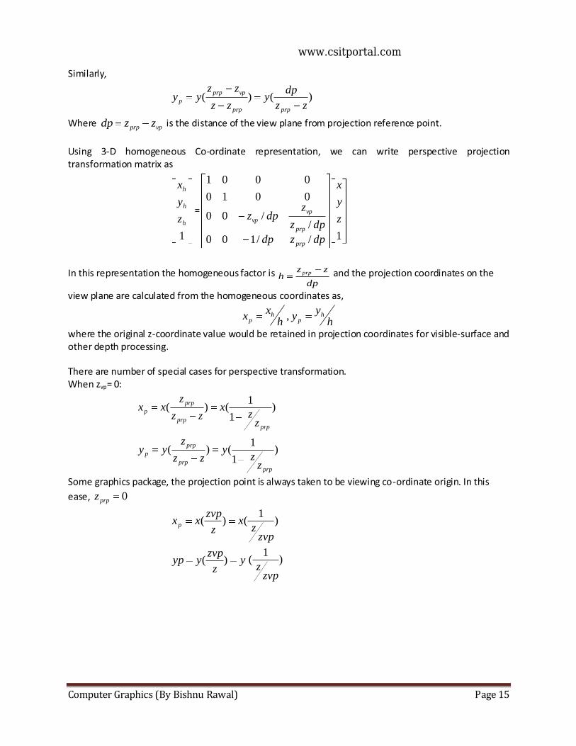
Computer Graphics (By Bishnu Rawal) Page 15
Similarly,
)()(zz
dpy
zz
zzyy
prpprp
vpprp
p
Where vpprp zzdp is the distance of the view plane from projection reference point.
Using 3-D homogeneous Co-ordinate representation, we can write perspective projection transformation matrix as
1
h
h
h
z
y
x
=
1//100
//00
0010
0001
z
y
x
dpzdp
dpz
zdpz
prp
prp
vp
vp
In this representation the homogeneous factor is dp
zzh
prp and the projection coordinates on the
view plane are calculated from the homogeneous coordinates as,
hy
yh
xx h
ph
p ,
where the original z-coordinate value would be retained in projection coordinates for visible-surface and other depth processing. There are number of special cases for perspective transformation. When zvp= 0:
)1
1()(
prpprp
prp
p
zz
xzz
zxx
)1
1()(
prpprp
prp
p
zz
yzz
zyy
Some graphics package, the projection point is always taken to be viewing co-ordinate origin. In this
ease, 0prpz
)1
()(
zvpz
xz
zvpxxp
yz
zvpyyp )( )
1(
zvpz
www.csitportal.com
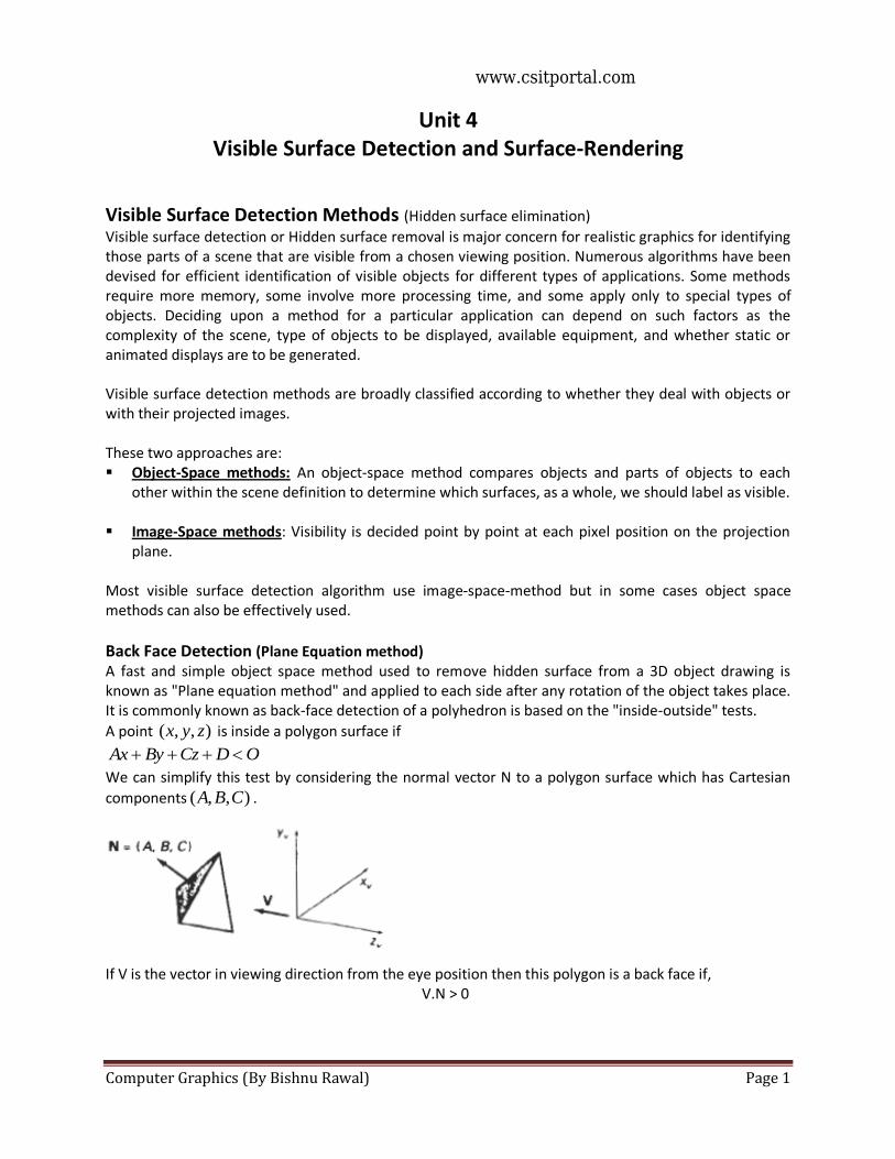
Computer Graphics (By Bishnu Rawal) Page 1
Unit 4 Visible Surface Detection and Surface-Rendering
Visible Surface Detection Methods (Hidden surface elimination) Visible surface detection or Hidden surface removal is major concern for realistic graphics for identifying those parts of a scene that are visible from a chosen viewing position. Numerous algorithms have been devised for efficient identification of visible objects for different types of applications. Some methods require more memory, some involve more processing time, and some apply only to special types of objects. Deciding upon a method for a particular application can depend on such factors as the complexity of the scene, type of objects to be displayed, available equipment, and whether static or animated displays are to be generated. Visible surface detection methods are broadly classified according to whether they deal with objects or with their projected images. These two approaches are: Object-Space methods: An object-space method compares objects and parts of objects to each
other within the scene definition to determine which surfaces, as a whole, we should label as visible. Image-Space methods: Visibility is decided point by point at each pixel position on the projection
plane. Most visible surface detection algorithm use image-space-method but in some cases object space methods can also be effectively used.
Back Face Detection (Plane Equation method) A fast and simple object space method used to remove hidden surface from a 3D object drawing is known as "Plane equation method" and applied to each side after any rotation of the object takes place. It is commonly known as back-face detection of a polyhedron is based on the "inside-outside" tests.
A point ),,( zyx is inside a polygon surface if
ODCzByAx
We can simplify this test by considering the normal vector N to a polygon surface which has Cartesian
components ),,( CBA .
If V is the vector in viewing direction from the eye position then this polygon is a back face if, V.N > 0
www.csitportal.com
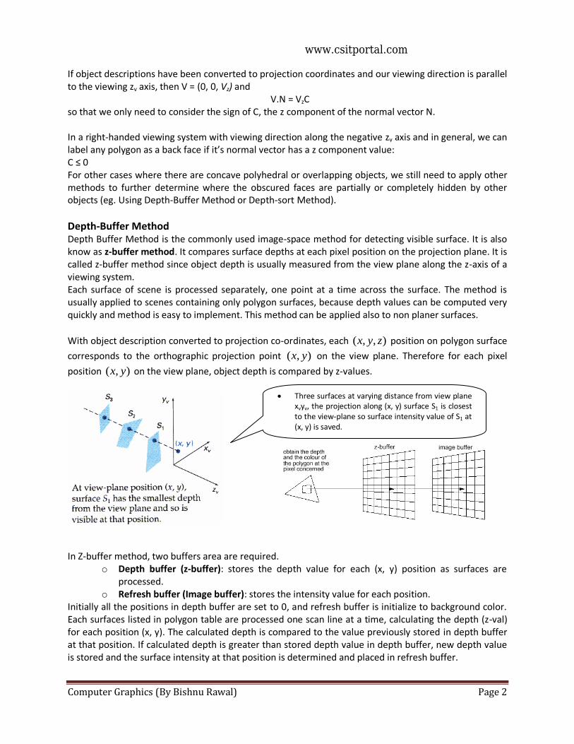
Computer Graphics (By Bishnu Rawal) Page 2
If object descriptions have been converted to projection coordinates and our viewing direction is parallel to the viewing zv axis, then V = (0, 0, Vz) and
V.N = VzC so that we only need to consider the sign of C, the z component of the normal vector N. In a right-handed viewing system with viewing direction along the negative zv axis and in general, we can label any polygon as a back face if it’s normal vector has a z component value: C ≤ 0 For other cases where there are concave polyhedral or overlapping objects, we still need to apply other methods to further determine where the obscured faces are partially or completely hidden by other objects (eg. Using Depth-Buffer Method or Depth-sort Method).
Depth-Buffer Method Depth Buffer Method is the commonly used image-space method for detecting visible surface. It is also know as z-buffer method. It compares surface depths at each pixel position on the projection plane. It is called z-buffer method since object depth is usually measured from the view plane along the z-axis of a viewing system. Each surface of scene is processed separately, one point at a time across the surface. The method is usually applied to scenes containing only polygon surfaces, because depth values can be computed very quickly and method is easy to implement. This method can be applied also to non planer surfaces.
With object description converted to projection co-ordinates, each ),,( zyx position on polygon surface
corresponds to the orthographic projection point ),( yx on the view plane. Therefore for each pixel
position ),( yx on the view plane, object depth is compared by z-values.
In Z-buffer method, two buffers area are required.
o Depth buffer (z-buffer): stores the depth value for each (x, y) position as surfaces are processed.
o Refresh buffer (Image buffer): stores the intensity value for each position. Initially all the positions in depth buffer are set to 0, and refresh buffer is initialize to background color. Each surfaces listed in polygon table are processed one scan line at a time, calculating the depth (z-val) for each position (x, y). The calculated depth is compared to the value previously stored in depth buffer at that position. If calculated depth is greater than stored depth value in depth buffer, new depth value is stored and the surface intensity at that position is determined and placed in refresh buffer.
Three surfaces at varying distance from view plane xvyv, the projection along (x, y) surface S1 is closest to the view-plane so surface intensity value of S1 at (x, y) is saved.
www.csitportal.com
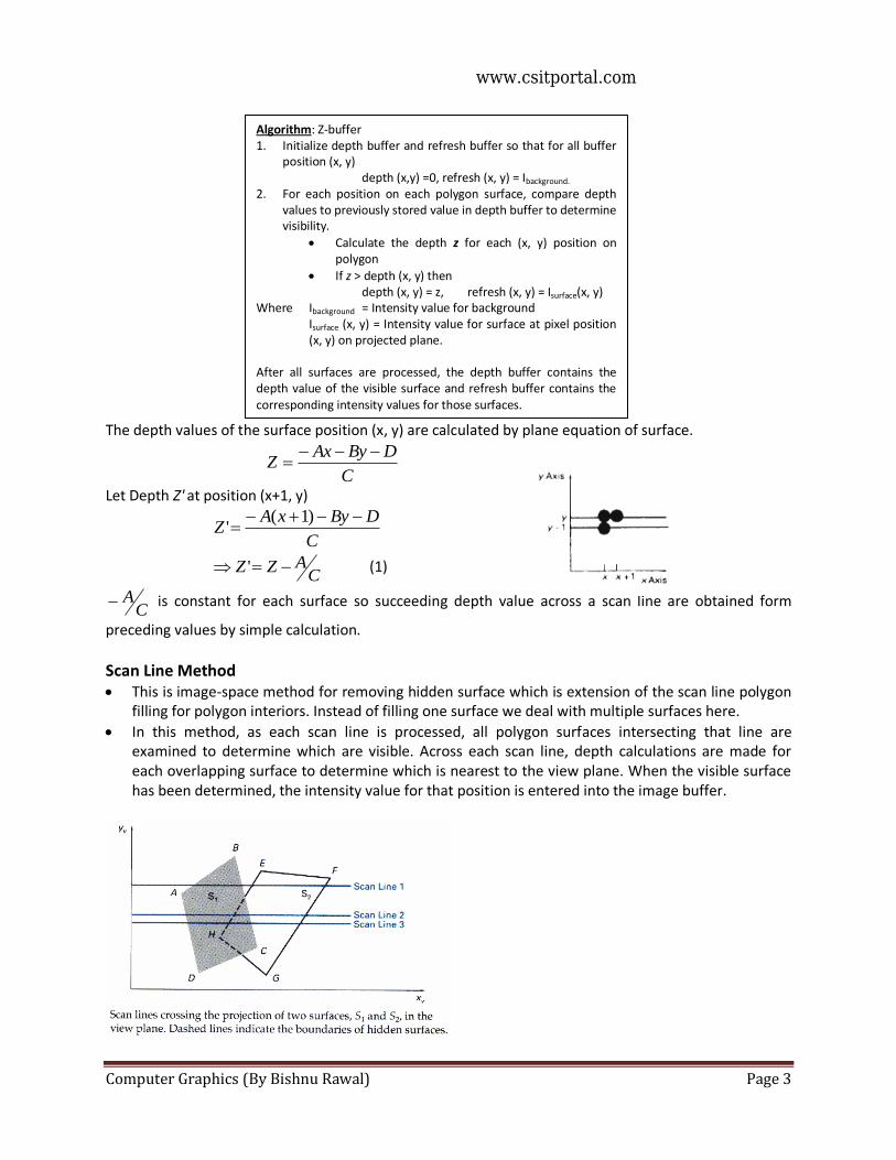
Computer Graphics (By Bishnu Rawal) Page 3
The depth values of the surface position (x, y) are calculated by plane equation of surface.
C
DByAxZ
Let Depth Z' at position (x+1, y)
C
DByxAZ
)1('
C
AZZ ' (1)
CA is constant for each surface so succeeding depth value across a scan line are obtained form
preceding values by simple calculation.
Scan Line Method This is image-space method for removing hidden surface which is extension of the scan line polygon
filling for polygon interiors. Instead of filling one surface we deal with multiple surfaces here.
In this method, as each scan line is processed, all polygon surfaces intersecting that line are examined to determine which are visible. Across each scan line, depth calculations are made for each overlapping surface to determine which is nearest to the view plane. When the visible surface has been determined, the intensity value for that position is entered into the image buffer.
Algorithm: Z-buffer 1. Initialize depth buffer and refresh buffer so that for all buffer
position (x, y) depth (x,y) =0, refresh (x, y) = Ibackground.
2. For each position on each polygon surface, compare depth values to previously stored value in depth buffer to determine visibility.
Calculate the depth z for each (x, y) position on polygon
If z > depth (x, y) then depth (x, y) = z, refresh (x, y) = Isurface(x, y) Where Ibackground = Intensity value for background
Isurface (x, y) = Intensity value for surface at pixel position (x, y) on projected plane.
After all surfaces are processed, the depth buffer contains the depth value of the visible surface and refresh buffer contains the corresponding intensity values for those surfaces.
www.csitportal.com
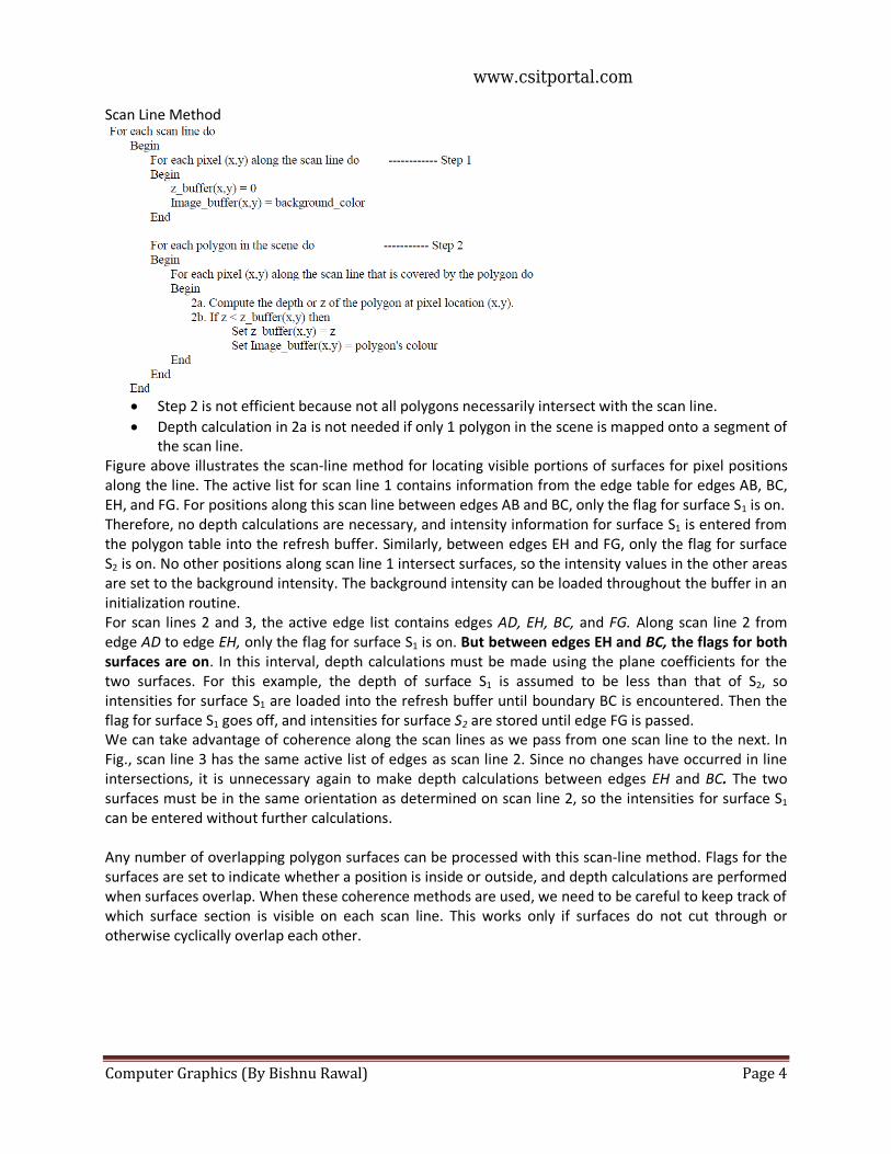
Computer Graphics (By Bishnu Rawal) Page 4
Scan Line Method
Step 2 is not efficient because not all polygons necessarily intersect with the scan line.
Depth calculation in 2a is not needed if only 1 polygon in the scene is mapped onto a segment of the scan line.
Figure above illustrates the scan-line method for locating visible portions of surfaces for pixel positions along the line. The active list for scan line 1 contains information from the edge table for edges AB, BC, EH, and FG. For positions along this scan line between edges AB and BC, only the flag for surface S1 is on. Therefore, no depth calculations are necessary, and intensity information for surface S1 is entered from the polygon table into the refresh buffer. Similarly, between edges EH and FG, only the flag for surface S2 is on. No other positions along scan line 1 intersect surfaces, so the intensity values in the other areas are set to the background intensity. The background intensity can be loaded throughout the buffer in an initialization routine. For scan lines 2 and 3, the active edge list contains edges AD, EH, BC, and FG. Along scan line 2 from edge AD to edge EH, only the flag for surface S1 is on. But between edges EH and BC, the flags for both surfaces are on. In this interval, depth calculations must be made using the plane coefficients for the two surfaces. For this example, the depth of surface S1 is assumed to be less than that of S2, so intensities for surface S1 are loaded into the refresh buffer until boundary BC is encountered. Then the flag for surface S1 goes off, and intensities for surface S2 are stored until edge FG is passed. We can take advantage of coherence along the scan lines as we pass from one scan line to the next. In Fig., scan line 3 has the same active list of edges as scan line 2. Since no changes have occurred in line intersections, it is unnecessary again to make depth calculations between edges EH and BC. The two surfaces must be in the same orientation as determined on scan line 2, so the intensities for surface S1 can be entered without further calculations. Any number of overlapping polygon surfaces can be processed with this scan-line method. Flags for the surfaces are set to indicate whether a position is inside or outside, and depth calculations are performed when surfaces overlap. When these coherence methods are used, we need to be careful to keep track of which surface section is visible on each scan line. This works only if surfaces do not cut through or otherwise cyclically overlap each other.
www.csitportal.com
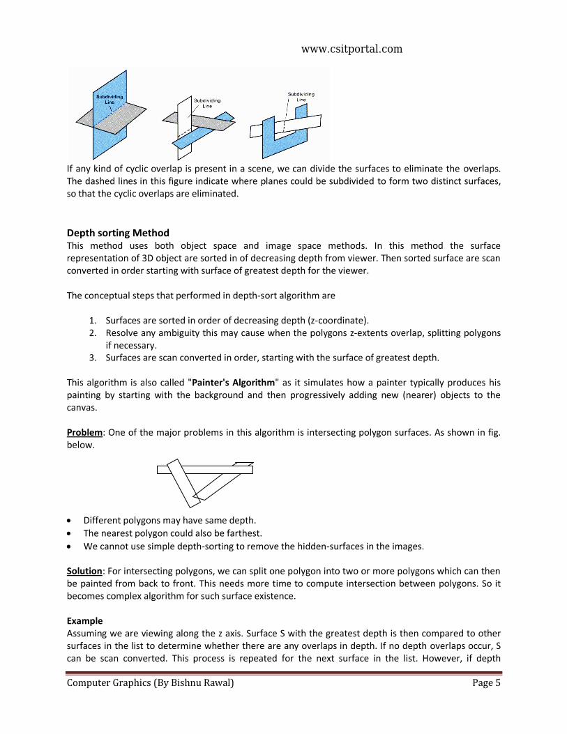
Computer Graphics (By Bishnu Rawal) Page 5
If any kind of cyclic overlap is present in a scene, we can divide the surfaces to eliminate the overlaps. The dashed lines in this figure indicate where planes could be subdivided to form two distinct surfaces, so that the cyclic overlaps are eliminated.
Depth sorting Method This method uses both object space and image space methods. In this method the surface representation of 3D object are sorted in of decreasing depth from viewer. Then sorted surface are scan converted in order starting with surface of greatest depth for the viewer. The conceptual steps that performed in depth-sort algorithm are
1. Surfaces are sorted in order of decreasing depth (z-coordinate). 2. Resolve any ambiguity this may cause when the polygons z-extents overlap, splitting polygons
if necessary. 3. Surfaces are scan converted in order, starting with the surface of greatest depth.
This algorithm is also called "Painter's Algorithm" as it simulates how a painter typically produces his painting by starting with the background and then progressively adding new (nearer) objects to the canvas. Problem: One of the major problems in this algorithm is intersecting polygon surfaces. As shown in fig. below.
Different polygons may have same depth.
The nearest polygon could also be farthest.
We cannot use simple depth-sorting to remove the hidden-surfaces in the images. Solution: For intersecting polygons, we can split one polygon into two or more polygons which can then be painted from back to front. This needs more time to compute intersection between polygons. So it becomes complex algorithm for such surface existence. Example Assuming we are viewing along the z axis. Surface S with the greatest depth is then compared to other surfaces in the list to determine whether there are any overlaps in depth. If no depth overlaps occur, S can be scan converted. This process is repeated for the next surface in the list. However, if depth
www.csitportal.com
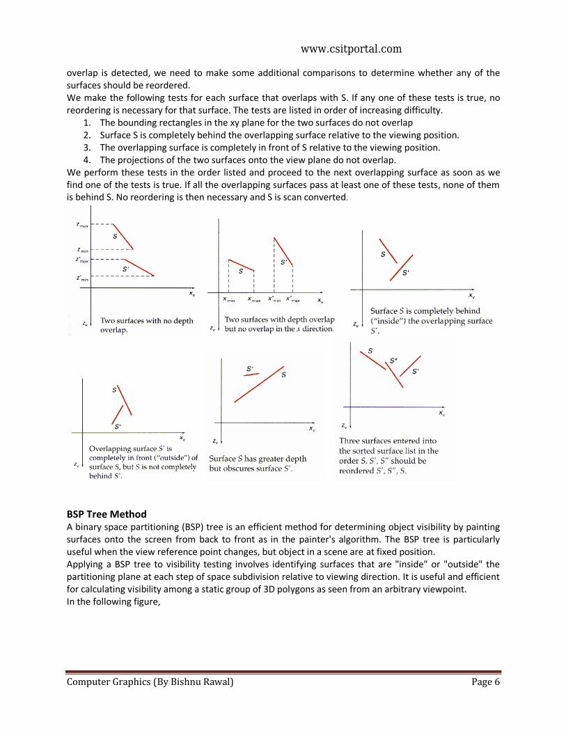
Computer Graphics (By Bishnu Rawal) Page 6
overlap is detected, we need to make some additional comparisons to determine whether any of the surfaces should be reordered. We make the following tests for each surface that overlaps with S. If any one of these tests is true, no reordering is necessary for that surface. The tests are listed in order of increasing difficulty.
1. The bounding rectangles in the xy plane for the two surfaces do not overlap 2. Surface S is completely behind the overlapping surface relative to the viewing position. 3. The overlapping surface is completely in front of S relative to the viewing position. 4. The projections of the two surfaces onto the view plane do not overlap.
We perform these tests in the order listed and proceed to the next overlapping surface as soon as we find one of the tests is true. If all the overlapping surfaces pass at least one of these tests, none of them is behind S. No reordering is then necessary and S is scan converted.
BSP Tree Method A binary space partitioning (BSP) tree is an efficient method for determining object visibility by painting surfaces onto the screen from back to front as in the painter's algorithm. The BSP tree is particularly useful when the view reference point changes, but object in a scene are at fixed position. Applying a BSP tree to visibility testing involves identifying surfaces that are "inside" or "outside" the partitioning plane at each step of space subdivision relative to viewing direction. It is useful and efficient for calculating visibility among a static group of 3D polygons as seen from an arbitrary viewpoint. In the following figure,
www.csitportal.com
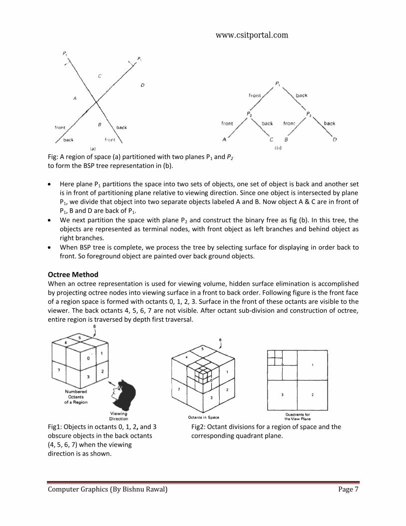
Computer Graphics (By Bishnu Rawal) Page 7
Fig: A region of space (a) partitioned with two planes P1 and P2 to form the BSP tree representation in (b).
Here plane P1 partitions the space into two sets of objects, one set of object is back and another set is in front of partitioning plane relative to viewing direction. Since one object is intersected by plane P1, we divide that object into two separate objects labeled A and B. Now object A & C are in front of P1, B and D are back of P1.
We next partition the space with plane P2 and construct the binary free as fig (b). In this tree, the objects are represented as terminal nodes, with front object as left branches and behind object as right branches.
When BSP tree is complete, we process the tree by selecting surface for displaying in order back to front. So foreground object are painted over back ground objects.
Octree Method When an octree representation is used for viewing volume, hidden surface elimination is accomplished by projecting octree nodes into viewing surface in a front to back order. Following figure is the front face of a region space is formed with octants 0, 1, 2, 3. Surface in the front of these octants are visible to the viewer. The back octants 4, 5, 6, 7 are not visible. After octant sub-division and construction of octree, entire region is traversed by depth first traversal.
Fig1: Objects in octants 0, 1, 2, and 3 Fig2: Octant divisions for a region of space and the obscure objects in the back octants corresponding quadrant plane. (4, 5, 6, 7) when the viewing direction is as shown.
www.csitportal.com
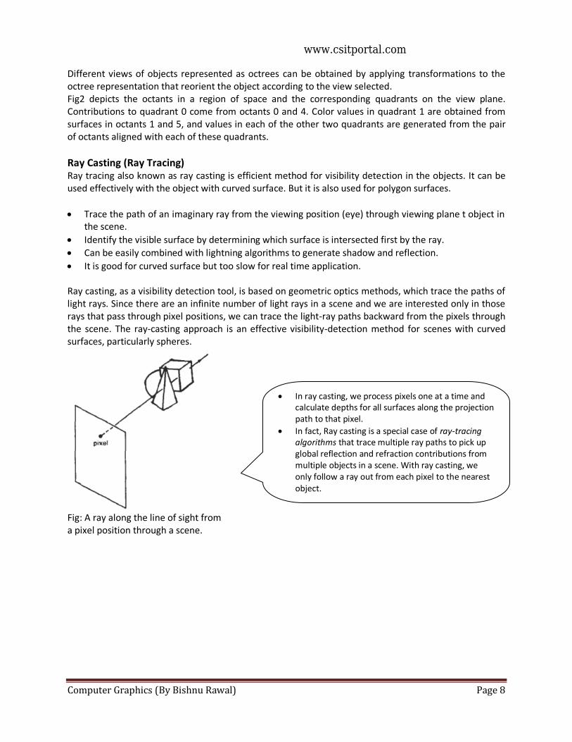
Computer Graphics (By Bishnu Rawal) Page 8
Different views of objects represented as octrees can be obtained by applying transformations to the octree representation that reorient the object according to the view selected. Fig2 depicts the octants in a region of space and the corresponding quadrants on the view plane. Contributions to quadrant 0 come from octants 0 and 4. Color values in quadrant 1 are obtained from surfaces in octants 1 and 5, and values in each of the other two quadrants are generated from the pair of octants aligned with each of these quadrants.
Ray Casting (Ray Tracing) Ray tracing also known as ray casting is efficient method for visibility detection in the objects. It can be used effectively with the object with curved surface. But it is also used for polygon surfaces.
Trace the path of an imaginary ray from the viewing position (eye) through viewing plane t object in the scene.
Identify the visible surface by determining which surface is intersected first by the ray.
Can be easily combined with lightning algorithms to generate shadow and reflection.
It is good for curved surface but too slow for real time application. Ray casting, as a visibility detection tool, is based on geometric optics methods, which trace the paths of light rays. Since there are an infinite number of light rays in a scene and we are interested only in those rays that pass through pixel positions, we can trace the light-ray paths backward from the pixels through the scene. The ray-casting approach is an effective visibility-detection method for scenes with curved surfaces, particularly spheres.
Fig: A ray along the line of sight from a pixel position through a scene.
In ray casting, we process pixels one at a time and calculate depths for all surfaces along the projection path to that pixel.
In fact, Ray casting is a special case of ray-tracing algorithms that trace multiple ray paths to pick up global reflection and refraction contributions from multiple objects in a scene. With ray casting, we only follow a ray out from each pixel to the nearest object.
www.csitportal.com
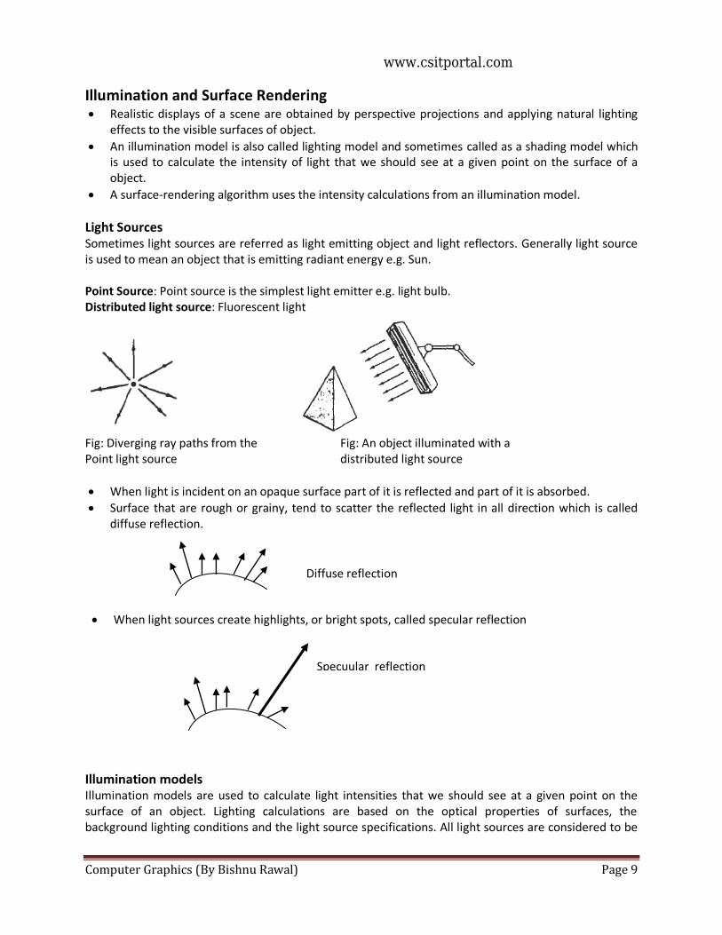
Computer Graphics (By Bishnu Rawal) Page 9
Illumination and Surface Rendering Realistic displays of a scene are obtained by perspective projections and applying natural lighting
effects to the visible surfaces of object.
An illumination model is also called lighting model and sometimes called as a shading model which is used to calculate the intensity of light that we should see at a given point on the surface of a object.
A surface-rendering algorithm uses the intensity calculations from an illumination model.
Light Sources Sometimes light sources are referred as light emitting object and light reflectors. Generally light source is used to mean an object that is emitting radiant energy e.g. Sun. Point Source: Point source is the simplest light emitter e.g. light bulb. Distributed light source: Fluorescent light
Fig: Diverging ray paths from the Fig: An object illuminated with a Point light source distributed light source
When light is incident on an opaque surface part of it is reflected and part of it is absorbed.
Surface that are rough or grainy, tend to scatter the reflected light in all direction which is called diffuse reflection.
When light sources create highlights, or bright spots, called specular reflection
Illumination models Illumination models are used to calculate light intensities that we should see at a given point on the surface of an object. Lighting calculations are based on the optical properties of surfaces, the background lighting conditions and the light source specifications. All light sources are considered to be
Specuular reflection
Diffuse reflection
www.csitportal.com
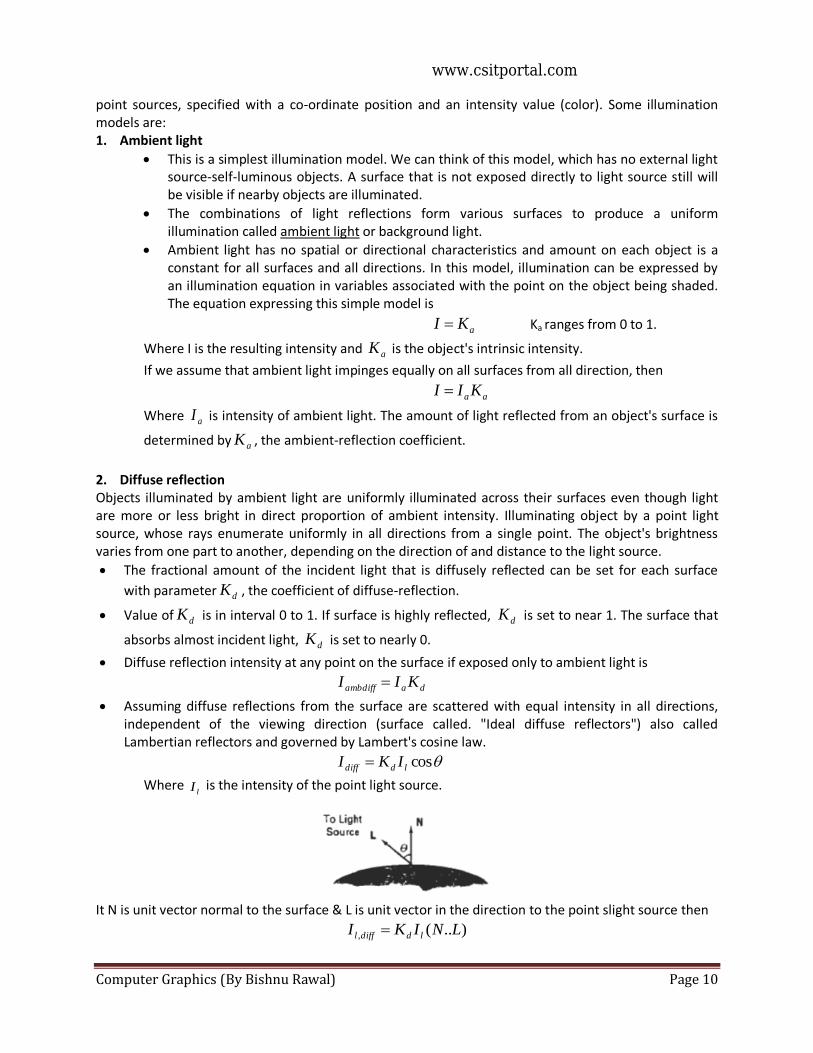
Computer Graphics (By Bishnu Rawal) Page 10
point sources, specified with a co-ordinate position and an intensity value (color). Some illumination models are: 1. Ambient light
This is a simplest illumination model. We can think of this model, which has no external light source-self-luminous objects. A surface that is not exposed directly to light source still will be visible if nearby objects are illuminated.
The combinations of light reflections form various surfaces to produce a uniform illumination called ambient light or background light.
Ambient light has no spatial or directional characteristics and amount on each object is a constant for all surfaces and all directions. In this model, illumination can be expressed by an illumination equation in variables associated with the point on the object being shaded. The equation expressing this simple model is
aKI Ka ranges from 0 to 1.
Where I is the resulting intensity and aK is the object's intrinsic intensity.
If we assume that ambient light impinges equally on all surfaces from all direction, then
aaKII
Where aI is intensity of ambient light. The amount of light reflected from an object's surface is
determined by aK , the ambient-reflection coefficient.
2. Diffuse reflection Objects illuminated by ambient light are uniformly illuminated across their surfaces even though light are more or less bright in direct proportion of ambient intensity. Illuminating object by a point light source, whose rays enumerate uniformly in all directions from a single point. The object's brightness varies from one part to another, depending on the direction of and distance to the light source.
The fractional amount of the incident light that is diffusely reflected can be set for each surface
with parameter dK , the coefficient of diffuse-reflection.
Value of dK is in interval 0 to 1. If surface is highly reflected, dK is set to near 1. The surface that
absorbs almost incident light, dK is set to nearly 0.
Diffuse reflection intensity at any point on the surface if exposed only to ambient light is
daambdiff KII
Assuming diffuse reflections from the surface are scattered with equal intensity in all directions, independent of the viewing direction (surface called. "Ideal diffuse reflectors") also called Lambertian reflectors and governed by Lambert's cosine law.
coslddiff IKI
Where lI is the intensity of the point light source.
It N is unit vector normal to the surface & L is unit vector in the direction to the point slight source then
)..(, LNIKI lddiffl
www.csitportal.com
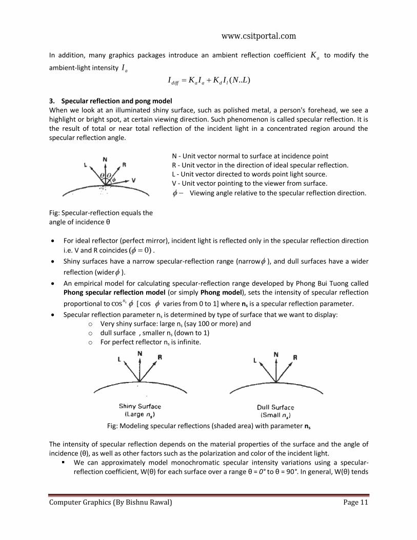
Computer Graphics (By Bishnu Rawal) Page 11
In addition, many graphics packages introduce an ambient reflection coefficient aK to modify the
ambient-light intensity aI
)..( LNIKIKI ldaadiff
3. Specular reflection and pong model When we look at an illuminated shiny surface, such as polished metal, a person's forehead, we see a highlight or bright spot, at certain viewing direction. Such phenomenon is called specular reflection. It is the result of total or near total reflection of the incident light in a concentrated region around the specular reflection angle.
N - Unit vector normal to surface at incidence point R - Unit vector in the direction of ideal specular reflection. L - Unit vector directed to words point light source. V - Unit vector pointing to the viewer from surface.
Viewing angle relative to the specular reflection direction.
Fig: Specular-reflection equals the angle of incidence θ
For ideal reflector (perfect mirror), incident light is reflected only in the specular reflection direction
i.e. V and R coincides )0( .
Shiny surfaces have a narrow specular-reflection range (narrow ), and dull surfaces have a wider
reflection (wider ).
An empirical model for calculating specular-reflection range developed by Phong Bui Tuong called Phong specular reflection model (or simply Phong model), sets the intensity of specular reflection
proportional to sncos [ cos varies from 0 to 1] where ns is a specular reflection parameter.
Specular reflection parameter ns is determined by type of surface that we want to display: o Very shiny surface: large ns (say 100 or more) and o dull surface , smaller ns (down to 1) o For perfect reflector ns is infinite.
Fig: Modeling specular reflections (shaded area) with parameter ns
The intensity of specular reflection depends on the material properties of the surface and the angle of incidence (θ), as well as other factors such as the polarization and color of the incident light.
We can approximately model monochromatic specular intensity variations using a specular-reflection coefficient, W(θ) for each surface over a range θ = 0° to θ = 90°. In general, W(θ) tends
www.csitportal.com
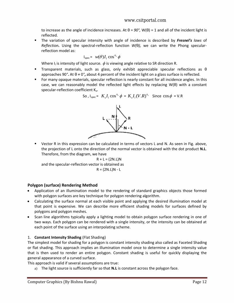
Computer Graphics (By Bishnu Rawal) Page 12
to increase as the angle of incidence increases. At θ = 90°, W(θ) = 1 and all of the incident light is reflected.
The variation of specular intensity with angle of incidence is described by Fresnel's laws of Reflection. Using the spectral-reflection function W(θ), we can write the Phong specular-reflection model as:
Ispec = sn
lIw cos)(
Where Il is intensity of light source. is viewing angle relative to SR direction R.
Transparent materials, such as glass, only exhibit appreciable specular reflections as θ approaches 90°. At θ = 0°, about 4 percent of the incident light on a glass surface is reflected.
For many opaque materials, specular reflection is nearly constant for all incidence angles. In this case, we can reasonably model the reflected light effects by replacing W(θ) with a constant specular-reflection coefficient Ks.
So , Ispec = sn
lsIK cos = sn
ls RVIK ).( Since cos = V.R
Vector R in this expression can be calculated in terms of vectors L and N. As seen in Fig. above,
the projection of L onto the direction of the normal vector is obtained with the dot product N.L. Therefore, from the diagram, we have
R + L = (2N.L)N and the specular-reflection vector is obtained as
R = (2N.L)N - L
Polygon (surface) Rendering Method Application of an illumination model to the rendering of standard graphics objects those formed
with polygon surfaces are key technique for polygon rendering algorithm.
Calculating the surface normal at each visible point and applying the desired illumination model at that point is expensive. We can describe more efficient shading models for surfaces defined by polygons and polygon meshes.
Scan line algorithms typically apply a lighting model to obtain polygon surface rendering in one of two ways. Each polygon can be rendered with a single intensity, or the intensity can be obtained at each point of the surface using an interpolating scheme.
1. Constant Intensity Shading (Flat Shading) The simplest model for shading for a polygon is constant intensity shading also called as Faceted Shading or flat shading. This approach implies an illumination model once to determine a single intensity value that is then used to render an entire polygon. Constant shading is useful for quickly displaying the general appearance of a curved surface. This approach is valid if several assumptions are true:
a) The light source is sufficiently far so that N.L is constant across the polygon face.
www.csitportal.com
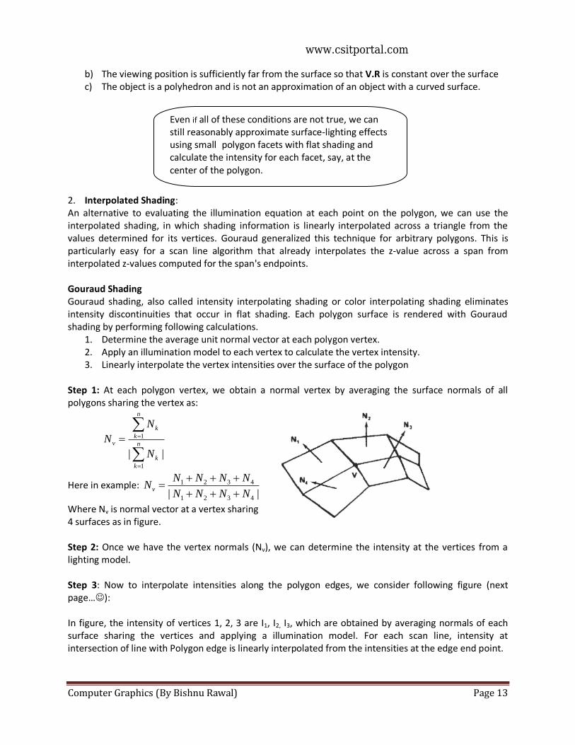
Computer Graphics (By Bishnu Rawal) Page 13
b) The viewing position is sufficiently far from the surface so that V.R is constant over the surface c) The object is a polyhedron and is not an approximation of an object with a curved surface.
2. Interpolated Shading: An alternative to evaluating the illumination equation at each point on the polygon, we can use the interpolated shading, in which shading information is linearly interpolated across a triangle from the values determined for its vertices. Gouraud generalized this technique for arbitrary polygons. This is particularly easy for a scan line algorithm that already interpolates the z-value across a span from interpolated z-values computed for the span's endpoints. Gouraud Shading Gouraud shading, also called intensity interpolating shading or color interpolating shading eliminates intensity discontinuities that occur in flat shading. Each polygon surface is rendered with Gouraud shading by performing following calculations.
1. Determine the average unit normal vector at each polygon vertex. 2. Apply an illumination model to each vertex to calculate the vertex intensity. 3. Linearly interpolate the vertex intensities over the surface of the polygon
Step 1: At each polygon vertex, we obtain a normal vertex by averaging the surface normals of all polygons sharing the vertex as:
||1
1
n
k
k
n
k
k
v
N
N
N
Here in example: || 4321
4321
NNNN
NNNNNv
Where Nv is normal vector at a vertex sharing 4 surfaces as in figure. Step 2: Once we have the vertex normals (Nv), we can determine the intensity at the vertices from a lighting model. Step 3: Now to interpolate intensities along the polygon edges, we consider following figure (next page…): In figure, the intensity of vertices 1, 2, 3 are I1, I2, I3, which are obtained by averaging normals of each surface sharing the vertices and applying a illumination model. For each scan line, intensity at intersection of line with Polygon edge is linearly interpolated from the intensities at the edge end point.
Even if all of these conditions are not true, we can still reasonably approximate surface-lighting effects using small polygon facets with flat shading and calculate the intensity for each facet, say, at the center of the polygon.
www.csitportal.com
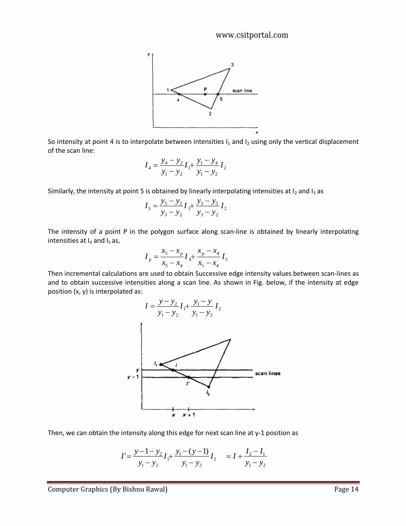
Computer Graphics (By Bishnu Rawal) Page 14
So intensity at point 4 is to interpolate between intensities I1 and I2 using only the vertical displacement of the scan line:
2
21
411
21
244 I
yy
yyI
yy
yyI
Similarly, the intensity at point 5 is obtained by linearly interpolating intensities at I2 and I3 as
2
23
533
23
255 I
yy
yyI
yy
yyI
The intensity of a point P in the polygon surface along scan-line is obtained by linearly interpolating intensities at I4 and I5 as,
5
45
4
4
45
5I
xx
xxI
xx
xxI
pp
p
Then incremental calculations are used to obtain Successive edge intensity values between scan-lines as and to obtain successive intensities along a scan line. As shown in Fig. below, if the intensity at edge position (x, y) is interpolated as:
2
21
11
21
2 Iyy
yyI
yy
yyI
Then, we can obtain the intensity along this edge for next scan line at y-1 position as
2
21
11
21
2 )1(1' I
yy
yyI
yy
yyI
21
12
yy
III
www.csitportal.com
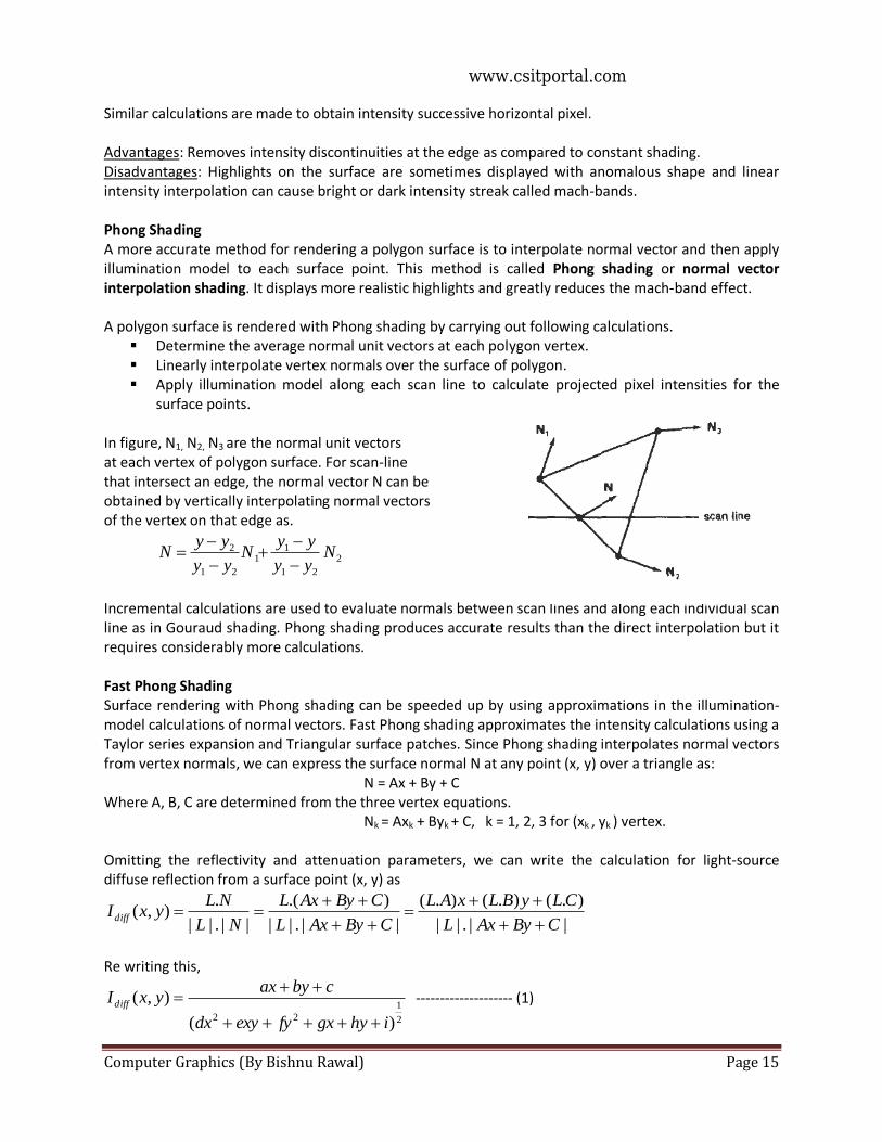
Computer Graphics (By Bishnu Rawal) Page 15
Similar calculations are made to obtain intensity successive horizontal pixel. Advantages: Removes intensity discontinuities at the edge as compared to constant shading. Disadvantages: Highlights on the surface are sometimes displayed with anomalous shape and linear intensity interpolation can cause bright or dark intensity streak called mach-bands. Phong Shading A more accurate method for rendering a polygon surface is to interpolate normal vector and then apply illumination model to each surface point. This method is called Phong shading or normal vector interpolation shading. It displays more realistic highlights and greatly reduces the mach-band effect. A polygon surface is rendered with Phong shading by carrying out following calculations.
Determine the average normal unit vectors at each polygon vertex. Linearly interpolate vertex normals over the surface of polygon. Apply illumination model along each scan line to calculate projected pixel intensities for the
surface points. In figure, N1, N2, N3 are the normal unit vectors at each vertex of polygon surface. For scan-line that intersect an edge, the normal vector N can be obtained by vertically interpolating normal vectors of the vertex on that edge as.
2
21
11
21
2 Nyy
yyN
yy
yyN
Incremental calculations are used to evaluate normals between scan lines and along each individual scan line as in Gouraud shading. Phong shading produces accurate results than the direct interpolation but it requires considerably more calculations. Fast Phong Shading Surface rendering with Phong shading can be speeded up by using approximations in the illumination-model calculations of normal vectors. Fast Phong shading approximates the intensity calculations using a Taylor series expansion and Triangular surface patches. Since Phong shading interpolates normal vectors from vertex normals, we can express the surface normal N at any point (x, y) over a triangle as:
N = Ax + By + C Where A, B, C are determined from the three vertex equations.
Nk = Axk + Byk + C, k = 1, 2, 3 for (xk , yk ) vertex. Omitting the reflectivity and attenuation parameters, we can write the calculation for light-source diffuse reflection from a surface point (x, y) as
||.||
).().().(
||.||
).(
||.||
.),(
CByAxL
CLyBLxAL
CByAxL
CByAxL
NL
NLyxIdiff
Re writing this,
2
1
22 )(
),(
ihygxfyexydx
cbyaxyxIdiff
-------------------- (1)
www.csitportal.com
Computer Graphics (By Bishnu Rawal) Page 16
Where parameters a, b, c, d… are used to represent the various dot products as ...||
.
L
NLa and so on
Finally, denominator of equation (1) can be expressed as Taylor series expansions and retains terms up to second degree in x and y. This yields
012
2
34
2
5),( TyTxTyTxyTxTyxIdiff
Where each Tk is a function of parameters a, b, c, d, and so forth. This method still takes twice as long as in Gouraud shading. Normal Phong shading takes six to seven times that of Gouraud shading.
www.csitportal.com
Computer Graphics (By Bishnu Rawal) Page 1
Unit 5 Computer Animation
Introduction Although we tend to think of animation as implying object motions, the term computer animation generally refers to any time sequence of visual changes in a scene. In addition to changing object position with translations or rotations, a computer-generated animation could display time variations in object size, color, transparency, or surface texture. Some typical applications of computer-generated animation are entertainment (motion pictures and cartoons), advertising, scientific and engineering studies, and training and education. Advertising animations often transition one object shape into another: for example, transforming a can of motor oil into an automobile engine. Computer animations can also be generated by changing camera parameters, such as position, orientation, and focal length. And we can produce computer animations by charging lighting effects or other parameters and procedures associated with illumination and rendering.
Design of animation sequences
In general, an animation sequence is designed with the following steps: 1. Storyboard layout 2. Object definitions 3. Key-frame specifications 4. Generation of in-between frames
This standard approach for animated cartoons is applied to other animation applications as well, although there are many special applications that do not follow this sequence. Real-time computer animations produced by flight simulators, for instance, display motion sequences in response to settings on the aircraft controls. For frame-by-frame animation, each frame of the scene is separately generated and stored. Later, the frames can be recorded on film or they can be consecutively displayed in "real-time playback" mode.
1. Storyboard is an outline of the action. It defines the motion sequence as a set of basic events that are to take place. Depending on the type of animation to be produced, the storyboard could consist of a set of rough sketches or it could be a list of the basic ideas for the motion.
2. An object definition is given for each participant in the action. Objects can be defined in terms of basic shapes, such as polygons or splines. In addition, the associated movements for each object are specified along with the shape.
3. A key frame is a detailed drawing of the scene at a certain time in the animation sequence. Within each key frame, each object is positioned according to the time for that frame. Some key frames are chosen at extreme positions in the action; others are spaced so that the time interval between key frames is not too great. More key frames are specified for intricate motions than for simple, slowly varying motions.
4. In-betweens are the intermediate frames between the key frames. The number of in-betweens needed is determined by the media to be used to display the animation. Film requires 24 frames per second, and graphics terminals are refreshed at the rate of 30 to 60 frames per second.
www.csitportal.com
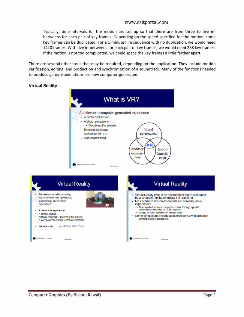
Computer Graphics (By Bishnu Rawal) Page 2
Typically, time intervals for the motion are set up so that there are from three to five in-betweens for each pair of key frames. Depending on the speed specified for the motion, some key frames can be duplicated. For a 1-minute film sequence with no duplication, we would need 1440 frames. With five in-betweens for each pair of key frames, we would need 288 key frames. If the motion is not too complicated, we could space the key frames a little farther apart.
There are several other tasks that may be required, depending on the application. They include motion verification, editing, and production and synchronization of a soundtrack. Many of the functions needed to produce general animations are now computer-generated.
Virtual Reality
www.csitportal.com
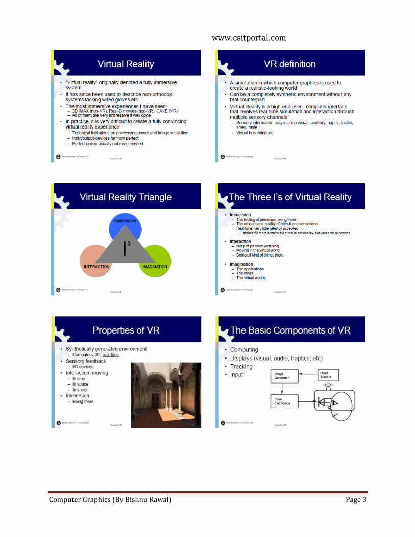
Computer Graphics (By Bishnu Rawal) Page 3
www.csitportal.com
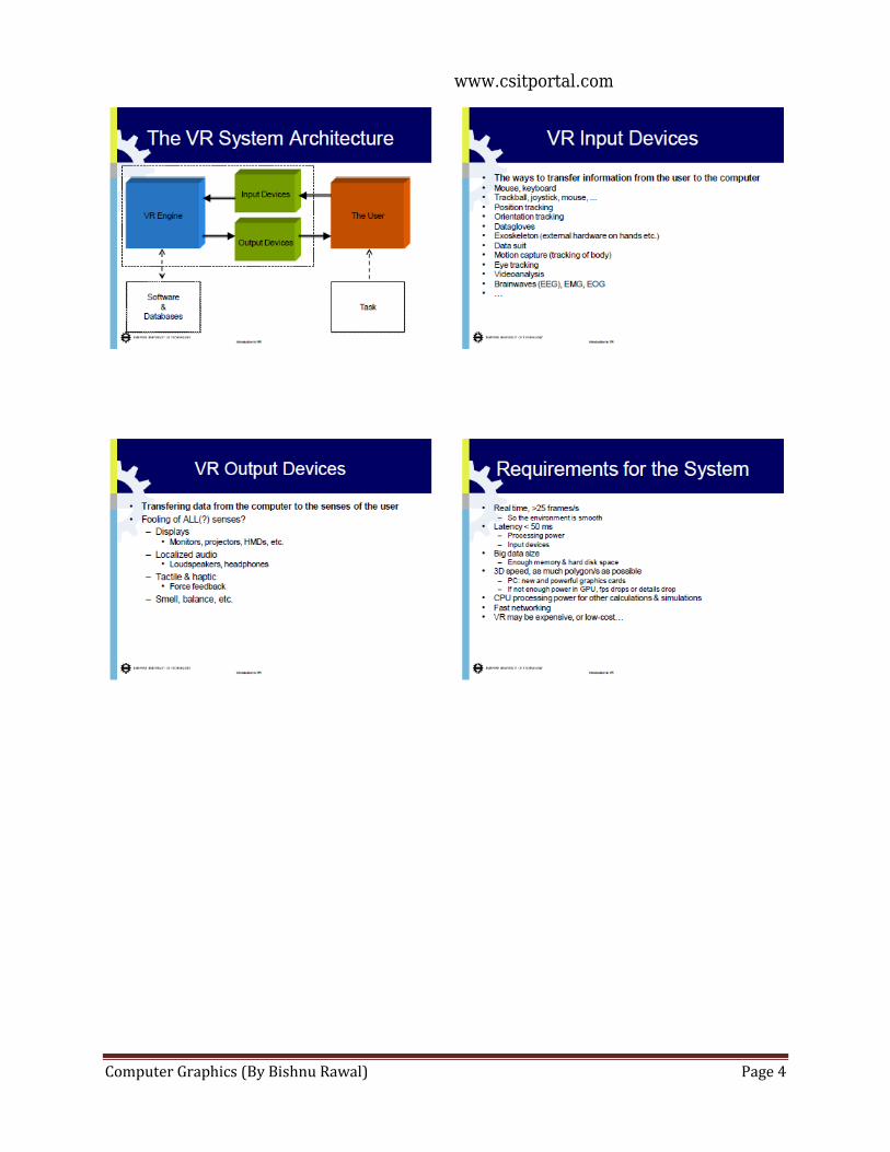
Computer Graphics (By Bishnu Rawal) Page 4
www.csitportal.com