Embed Size (px)
Citation preview

Quantitative Methods 1
Unit 1 Mathematics In Management
Learning Outcome
After reading this unit, you will be able to:
• Analyse major business activities using mathematics and statistics
• Identify scope and significance of business mathematics and statistics
• Explain functions
• Define and use notations and solve applications of functions
• Identify special functions
Time Required to Complete the unit
1. 1st
Reading: It will need 3 Hrs for reading a unit
2. 2nd Reading with understanding: It will need 4 Hrs for reading and understanding a
unit
3. Self Assessment: It will need 3 Hrs for reading and understanding a unit
4. Assignment: It will need 2 Hrs for completing an assignment
5. Revision and Further Reading: It is a continuous process
Content Map
1.1 Introduction
1.2 Business Mathematics and Business Statistics
1.2.1 Business Mathematics
1.2.2 Business Statistics
1.3 Scope and Importance of Mathematics in Managerial Decisions
1.4 Functions-Concept

2 Quantitative Methods
1.4.1 Definition of a Function
1.4.2 Notation
1.4.3 The Vertical Line Test
1.5 Application of Functions
1.6 Special Functions
1.6.1 Tables of Special Functions
1.6.2 Notations used in Special Functions
1.6.3 Evaluation of Special Functions
1.6.4 Kinds of Functions
1.7 Summary
1.8 Self Assessment Test
1.9 Further Reading
Quantitative Methods 3
1.1 Introduction
Quantitative methods are research techniques that are inevitably used to table
quantitative data i.e. information dealing with numbers and anything that is measurable.
Statistics, tables and graphs are the tools used to represent the results of these methods.
They must therefore be distinctly distinguished from qualitative methods.
In most physical and biological sciences, the use of either quantitative or qualitative
methods is uncontroversial and each is used when appropriate. In the social sciences,
particularly in sociology, social anthropology and psychology, the use of one or other type of
method has become a matter of controversy and even ideology, with particular schools of
thought within each discipline favouring one type of technique and rejecting the other.
Advocates of the quantitative methods are of the view that only by using such methods can
the social sciences become truly scientific, while advocates of qualitative methods argue
that quantitative methods tend to obscure the reality of the social phenomena under study
because they underestimate or neglect the non-measurable factors, which may be of utmost
importance. The modern tendency (and in reality the majority tendency throughout the
history of social science) is to use eclectic approaches. Quantitative methods might be used
with a global qualitative frame. Qualitative methods might be used to understand the
meaning of the numbers produced by quantitative methods. Using quantitative methods, it
is possible to give a precise and testable expression to qualitative ideas. This combination of
quantitative and qualitative data gathering is often referred to as mixed-methods research.
Mathematics is an essential subject and knowledge of it enhances a person's
reasoning, problem-solving skills and in general, ability to think logically. Hence it enables an
easy grasp of most subjects, whether science and technology, medicine, the economy or
business and finance. Mathematical tools and techniques such as the Theory of Chaos are
used for mapping and forecasting market trends. Statistics and probability, which are very
important branches of mathematics, are used in everyday business and economics.
Mathematics also forms an indispensible part of accounting and many accountancy
companies prefer graduates with dual degrees with mathematics, rather than just an
accountancy qualification. Financial mathematics and business mathematics are considered
two important branches of mathematics in today's world and these are examples of the
direct application of mathematics to business and economics. Examples of applied maths
such as probability theory and management science, queuing theory, time-series analysis,
linear programming all are vital for business.
In 1967, Stafford Beer characterised the field of management science as "the
business use of operations research". However, in modern times the term management

4 Quantitative Methods
science may also be used to refer to the separate fields of organisational studies or
corporate strategy. Like operational research itself, management science (MS) is an
interdisciplinary branch of applied mathematics devoted to optimal decision planning with
strong links with economics, business, engineering and other sciences. It uses various
scientific research-based principles, strategies and analytical methods including
mathematical modelling, statistics and numerical algorithms to improve an organisation's
ability to enact rational and meaningful management decisions by arriving at optimal or near
optimal solutions to complex decision problems. In short, management sciences help
businesses to achieve their goals using the scientific methods of operational research.
The management scientist's mandate is to use rational, systematic, science-based
techniques to inform and improve decisions of all kinds. Of course, the techniques of
management science are not restricted to business applications and may be applied to
military, medical, public administration, charitable groups, political groups or community
groups.
Management science is concerned with developing and applying models and
concepts that may prove useful in helping to elucidate management issues and solve
managerial problems, as well as designing and developing new and better models of
organisational excellence.
The application of these models within the corporate sector became known as
management science.
1.2 Business Mathematics and Business Statistics
1.2.1 BUSINESS MATHEMATICS
Business mathematics is mathematics used by commercial enterprises to record and
manage business operations. Commercial organisations use mathematics in accounting,
inventory management, marketing, sales forecasting and financial analysis. Mathematics
typically used in commerce includes elementary arithmetic, elementary algebra, statistics
and probability. Business management can be made more effective by the use of more
advanced mathematics such as calculus, matrix algebra and linear programming.
Another meaning of business mathematics, sometimes called commercial math or
consumer math, is a group of practical subjects used in commerce and everyday life.

Quantitative Methods 5
1.2.2 BUSINESS STATISTICS
Business statistics is the science of good decision making in the face of uncertainty. It
is used in many disciplines such as financial analysis, econometrics, auditing, production and
operations including services improvement and marketing research. These sources feature
regular repetitive publication of a series of data. This makes the topic of time series
especially important for business statistics. It is also a branch of applied statistics working
mostly on data collected as a by-product of doing business or by government agencies. It
provides knowledge and skills to interpret and use statistical techniques in a variety of
business applications. A typical business statistics course is intended for business majors and
covers statistical study, descriptive statistics (collection, description, analysis and summary
of data), probability and the binomial and normal distributions, test of hypotheses and
confidence intervals, linear regression and correlation.
Fig.1.1: Graph showing BSE Sensex through the Week Sep 20 to Sep 26' 2010
Study Notes

6 Quantitative Methods
Assessment
Differentiate between Business Mathematics and Business Statistics.
Discussion
Discuss the history of Quantative Techniques and their application in Management.
1.3 Scope and Importance of Mathematics in Managerial
Decisions
Mathematics is an integral aspect of our daily life. Many executive jobs such as those
of business consultants, computer consultants, airline pilots, company directors and a host
of others find that they require a solid understanding of basic mathematics and in some
cases require detailed knowledge of mathematics. It also plays an important role in business,
like business mathematics by commercial enterprises to record and manage business
operations.
Mathematics typically used in commerce includes, elementary arithmetic such as
fractions, decimals and percentages, elementary algebra, statistics and probability. Business
management can be made more effective in some cases by the use of more advanced
mathematics such as calculus, matrix algebra and linear programming. Commercial
organisations use mathematics in accounting, inventory management, marketing, sales
forecasting and financial analysis.
The practical applications typically include checking accounts, price discounts,
markups and markdowns, payroll calculations, simple and compound interest, consumer and
business credit and mortgages. For example, while computational formulas are covered in
most study-material on interest and mortgages, the use of prepared tables based on those
formulas is also presented and emphasised. Mathematics can provide a powerful support
for business decisions. Mathematics provides many important tools for economics and other
business fields.

Quantitative Methods 7
Why do business consultants and directors need to know math?
Business is all about selling a product or service to make money. All transactions
within a business have to be recorded in the company accounts and quite often involve large
sums of money. So, for example, you need to be able to estimate the effect of changing
numbers in the accounts when trying to work out your expected performance for the next
year. Also, businesses rely heavily on using percentages, in particular, anyone who works as
a sales person has to be quick at mental math, approximation and in working out
percentages. The more percentage discount you give a customer when you sell them a
product, the less profit your company will make (and quite often the less you will be paid!),
so it really does pay to know your math. If you work as a sales assistant, in many stores you
need to be efficient enough to calculate the cost of goods and charge the customers as
required without using the calculator. Businesses like to know that you can cope if the
machines break down and also, they believe that you can give better customer service if you
can respond to customers who know their mathematics. Here is an example of a letter
which often appears in local newspapers as "…I bought 2 of the same item at a shop priced
at Rs3.00 and gave the young sales assistant a Rs10 note and a Re1 coin, expecting to get a
Rs 5 note as change and do my bit to help prevent the store from running out of change. To
my amazement the sales assistant insisted that I had paid too much, I tried to explain to no
avail but in the end reluctantly took back my Re1 coin and was given 4 more Re1 coins as
change". Finally, there are jobs where you can escape from using any math at all refuse
collector, building labourer, farm hand etc. However, when you invest your hard earned
cash in the bank or building society or get a loan, how do you know that you are not being
taken advantage of? You need to use math to calculate compound interest rates (to see how
much your savings can grow). You also need to use math to understand the monthly
percentages, which are added to your credit cards or bank loans or you could end up paying
Rs.10, 000 in 5 year’s time for borrowing Rs 2,000 today. This is a good reason to understand
business mathematics.
In short, we can conclude that managers need to know mathematics and statistics to
take business decisions after analysing the present scenarios and then deciding on the basis
of these results. A general example can be quoted to explain this further.
(Reference: Business Standard-Monday, 27 Sept, 2010)
It may seem like a natural progression, but it has taken more than a decade-and-a-
half for telecom operators to look at the mobile phone business in India. This is because,
earlier, the market was completely skewed towards global manufacturers like Nokia, Sony
Ericsson and Samsung. However, the recent entry and growth of national mobile brands like

8 Quantitative Methods
Micromax, Maxx, Lava, Rage and GVL has helped many understand that the Nokias of this
world can be beaten in a price-sensitive market like India.
So, the first step from being a cell service operator to a mobile phone player was
taken by none other than the telecom giant Bharti Airtel when it announced the launch of its
own range of low-priced phones. This was launched under their subsidiary phone brand
company Beetel.
The price range of these mobile phones is between Rs 1,750 and Rs 7,000. After
Bharti, others have followed the cue. Tata Indicom recently announced a QWERTY phone,
which is a co-branded product with Alcatel. The mobile phone is bundled with Yahoo
services.
This is clearly pointing towards a trend of telecom operators looking towards the
mobile phone market for revenue growth. India does about 130- odd million in new mobile
phone sales each year and, with large subscribers now coming from the semi-urban to rural
areas, low-cost handsets seem to be the order of the day. Local players like Micromax
seemed to have cracked this aspect with their competitive price (ranging between Rs 2,000
and Rs 8,000) and an excellent bundle of features that includes social networking, among
other things.
Opportunity for Telecom Operators
As telecom penetration goes rural, telecom service giants like Bharti Airtel have the
unique advantage of a retail reach that mobile phone manufacturers are unlikely to have.
The other advantage they have is the option to bundle cheap call rates and plans along with
a mobile phone sale. They can also partner with content providers for value-added services
(VAS) products and bundle the same, targeting apps for rural India.
This is also their way to offset the impending losses that they may foresee due to the
increase tariff-based competition in the mobile services business and also the ever-falling
per-second rates.
All in all, it’s a natural progression for a telecom player to look at the Indian mobile
phones business as the market has already been expanded by existing Indian players via
their cheap pricing and feature rich phones.

Quantitative Methods 9
Study Notes
Assessment
Why do business consultants and directors need to know math? Give examples.
Discussion
Discuss the scope and importance of mathematics in managerial decisions
1.4 Functions- Concept
The mathematical concept of a function expresses the intuitive idea that one
quantity (the argument of the function, also known as the input) completely determines
another quantity (the value or the output). A function assigns a unique value to each input
of a specified type. The argument and the value may be real numbers, but they can also be
elements from any given sets, the domain and the co-domain of the function. An example of
a function with the real numbers as both its domain and co-domain is the function f(x) = 2x,
which assigns to every real number the real number with twice its value. In this case, it is
written that f(5) = 10.

10 Quantitative Methods
Fig. 1.2: Graph of Function
Graph of example function,
Both the domain and the range in the picture are the set of real numbers between -1
and 1.5.
In addition to elementary functions on numbers, functions include maps between
algebraic structures like groups and maps between geometric objects. In the abstract set-
theoretic approach, a function is a relation between the domain and the co-domain that
associates each element in the domain with exactly one element in the co-domain. An
example of a function with domain {A,B,C} and co-domain {1,2,3} associates A with 1, B with
2 and C with 3.
There are many ways to describe or represent functions: by a formula, by an
algorithm that computes it, by a plot or a graph. A table of values is a common way to
specify a function in statistics, physics, chemistry and other sciences. A function may also be
described through its relationship to other functions, for example, as the inverse function or
a solution of a differential equation. There are many different functions from the set of
natural numbers to itself, most of which cannot be expressed with a formula or an
algorithm.
In a setting where they have numerical outputs, functions may be added and
multiplied, yielding new functions. Collections of functions with certain properties, such as
continuous functions and differentiable functions, usually required to be closed under
certain operations are called function spaces and are studied as objects in their own right in
disciplines like real analysis and complex analysis. An important operation on functions,
which distinguishes them from numbers, is the composition of functions.

Quantitative Methods 11
Many traditions have sprouted around the use of functions because of their wide
usage. The symbol for the input to a function is often called the independent variable or
argument and is often represented by the letter x or if the input is a particular time by the
letter t. The symbol for the output is called the dependent variable or value and is often
represented by the letter y. The function itself is most often called f and thus the notation
y = f(x) indicates that a function named f has an input named x and an output named y.
Fig. 1.3: Function ƒ
A function ƒ takes an input, x and returns an output ƒ(x). One metaphor describes
the function as a 'machine' or 'black box' that converts the input into the output.
The set of all permitted inputs to a given function is called the domain of the
function. The set of all resulting outputs is called the image or range of the function. The
image is often a subset of some larger set and is called the co-domain of a function. Thus, for
example, the function f(x) = x2 could take as its domain the set of all real numbers, as its
image, the set of all non-negative real numbers and as its co-domain the set of all real
numbers. In that case, we would describe f as a real-valued function of a real variable.
Sometimes, especially in computer science, the term 'range' refers to the co-domain rather
than the image, so care needs to be taken when using the word.
It is usual practice in mathematics to introduce functions with temporary names like
ƒ. For example, ƒ(x) = 2x+1, implies ƒ (3) = 7; when a name for the function is not needed,
the form y = 2x+1 may be used. If a function is used often, it may be given a more
permanent name, for example,
Functions need not act on numbers: the domain and co-domain of a function may be
arbitrary sets. One example of a function that acts on non-numeric inputs takes English
words as inputs and returns the first letter of the input word as output. Furthermore,
functions need not be described by any expression, rule or algorithm: indeed, in some cases
12 Quantitative Methods
it may be impossible to define such a rule. For example, the association between inputs and
outputs in a choice function often lacks any fixed rule, although each input element is still
associated to one and only one output.
A function of two or more variables is considered in formal mathematics as having a
domain consisting of ordered pairs or triples of the argument values. For example, Sum(x,y)
= x+y operating on integers is the function- sum with a domain consisting of pairs of
integers. Sum then has a domain consisting of elements like (3, 4), a co-domain of integers
and an association between the two that can be described by a set of ordered pairs like
((3,4), 7). Evaluating Sum (3,4) then gives the value 7 associated with the pair (3,4).
A family of objects indexed by a set is equivalent to a function. For example, the
sequence 1, 1/2, 1/3, ..., 1/n, ... can be written as the ordered sequence <1/n> where n is a
natural number or as a function f(n) = 1/n from the set of natural numbers into the set of
rational numbers.
Dually, a subjective function partitions its domain into disjoint sets indexed by the
co-domain. This partition is known as the kernel of the function and the parts are called the
fibers or level sets of the function at each element of the co-domain. (A non-subjective
function divides its domain into disjoint and possibly-empty subsets).
1.4.1 DEFINITION OF A FUNCTION
A function is a rule that assigns to each element x from a set known as the 'domain' a
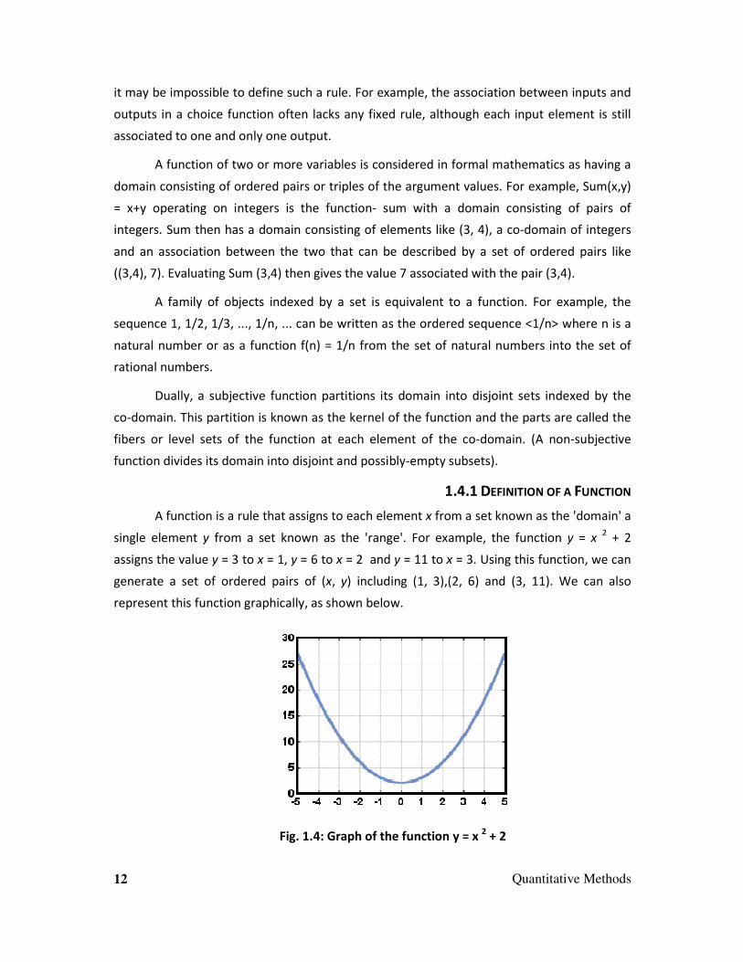
single element y from a set known as the 'range'. For example, the function y = x 2 + 2
assigns the value y = 3 to x = 1, y = 6 to x = 2 and y = 11 to x = 3. Using this function, we can
generate a set of ordered pairs of (x, y) including (1, 3),(2, 6) and (3, 11). We can also
represent this function graphically, as shown below.
Fig. 1.4: Graph of the function y = x 2 + 2

Quantitative Methods 13
One precise definition of a function is that it consists of an ordered triple of sets
which may be written as (X, Y, F). X is the domain of the function, Y is the co-domain and F is
a set of ordered pairs. In each of these ordered pairs (a, b), the first element a is from the
domain, the second element b is from the co-domain and every element in the domain is
the first element in one and only one ordered pair. The set of all b is known as the image of
the function. Some authors use the term "range" to mean the image, others to mean the co-
domain.
The notation ƒ:X→Y indicates that ƒ is a function with domain X and co-domain Y.
In most practical situations, the domain and co-domain are understood from context
and only the relationship between the input and output is given. Thus
is usually written as
The graph of a function is its set of ordered pairs. Such a set can be plotted on a pair
of coordinate axes. For example, (3, 9) is the point of intersection of the lines x = 3 and y = 9.
A function is a special case of a more general mathematical concept, the relation, for
which the restriction that each element of the domain appear as the first element in one
and only one ordered pair is removed (or, in other words, the restriction that each input be
associated to exactly one output). A relation is 'single-valued' or 'functional' when for each
element of the domain set the graph contains at most one ordered pair (and possibly none)
with it as a first element. A relation is called 'left-total' or simply 'total' when for each
element of the domain, the graph contains at least one ordered pair with it as a first
element (and possibly more than one). A relation that is both left-total and single-valued is a
function.
In some parts of mathematics, including Recursion Theory and functional analysis, it
is convenient to study partial functions in which some values of the domain have no
association in the graph, i.e. single-valued relations. For example, the function f such that
f(x) = 1/x does not define a value for x = 0 and thus is only a partial function from the real
line to the real line. The term total function can be used to stress the fact that every element
of the domain does appear as the first element of an ordered pair in the graph. In other
parts of mathematics, non-single-valued relations are similarly conflated with functions:

14 Quantitative Methods
these are called multi-valued functions, with the corresponding term single-valued function
for ordinary functions.
Some authors (especially in set theory) define a function as simply its graph f, with
the restriction that the graph should not contain two distinct ordered pairs with the same
first element. Indeed, given such a graph, one can construct a suitable triple by taking the
set of all first elements as the domain and the set of all second elements as the co-domain:
this automatically causes the function to be total and subjective. However, most authors in
advanced mathematics outside of set theory prefer the greater power of expression
afforded by defining a function as an ordered triple of sets.
Many operations in set theory- such as the power set- have the class of all sets as
their domain, therefore, although they are informally described as functions, they do not fit
the set-theoretical definition above outlined.
1.4.2 NOTATION
Formal description of a function typically involves the function's name, its domain, its
co-domain and a rule of correspondence. Thus, we frequently see a two-part notation, an
example being
Where the first part is read:
• 'ƒ is a function from N to R' (one often writes informally 'Let ƒ: X → Y' to mean 'Let ƒ be a
function from X to Y') or
• 'ƒ is a function on N into R' or
• 'ƒ is an R-valued function of an N-valued variable',
and the second part is read:
• maps to
• Here, the function named 'ƒ' has the natural numbers as domain, the real numbers as
co-domain and maps n to itself divided by π. Less, formally, this long form might be
abbreviated

Quantitative Methods 15
Where f(n) is read as 'f as function of n' or 'f of n'. There is some loss of information:
we are no longer explicitly given the domain N and co-domain R.
It is common to omit the parentheses around the argument when there is little
chance of confusion, thus: sin x; this is known as prefix notation. Writing the function after
its argument, as in x ƒ, is known as postfix notation; for example, the factorial function is
customarily written n!, even though its generalisation, the gamma function, is written Γ(n).
Parentheses are still used to resolve ambiguities and denote precedence, though in some
formal settings the consistent use of either prefix or postfix notation eliminates the need for
any parentheses.
1.4.3 THE VERTICAL LINE TEST
In the graph, each element x is assigned a single value y. If a rule assigned more than
one value y to a single element x, that rule could not be considered a function. As you may
recall from previous calculation, we can carry out a test for this property by using the
vertical line test, where we see whether we can draw a vertical line that passes through
more than one point on the graph:
Fig. 1.5: Vertical line test on the function y = x 2 + 2
It is assumed that because any vertical line would pass through only one point, y = x 2
+ 2 must be assigning only one y value to each x value and it therefore passes the vertical
line test. Thus, y = x 2 + 2 can rightfully be considered a function.
Study Notes

16 Quantitative Methods
Assessment
1. Explain the concept, meaning and definition of a function.
2. Explain in detail:
Discussion
Discuss, what do you understand by vertical line test.
1.5 Application of Functions
Application of functions can be cited from the following basic examples. These are
the examples of applications of functions where quantities such as area, perimeter, chord
etc are expressed as function of a variable.
Problem 1: A right triangle has one side x and a hypotenuse of 10 metres. Find the area of
the triangle as a function of x.
Solution to Problem 1:
If the sides of a right triangle are x and y, the area A of the triangle is given by
A = (1 / 2) x * y
We now need to express y in terms of x using the hypotenuse, side x and
Pythagoras's theorem
10 2 = x 2 + y 2
y = sq rt [100 - x 2]
Substitute y by its expression in the area formula to obtain
A(x) = (1 / 2) x sq rt [100 - x 2 ]
Problem 2: A rectangle has an area equal to 100 cm2 and a width x. Find the perimeter as a

Quantitative Methods 17
function of x.
Solution to Problem 2:
If x and y are the dimensions of the rectangle, using the formula of the area we
obtain
100 = x * y
The perimeter P is given by
P = 2(x + y)
Solve the equation 100 = x * y for y and substitute y in the formula for the perimeter
P(x) = 2(x + 100 / x)
Problem 3: Find the area of a square as a function of its perimeter x.
Solution to Problem 3:
The area of a square of side L is given by
A = L 2
The perimeter x of a square with side L is given by
x = 4 L
Solve the above for L and substitute in the area formula A above
A(x) = (x/4) 2 = x 2 / 16
Problem 4: A right circular cylinder has a radius r and a height equal to twice r. Find the
volume of the cylinder as a function of r.
Solution to Problem 4:
The volume V of a right circular cylinder is given by
V = (area of base of cylinder) * (height of cylinder)
= π * r 2 * (2 r)
= 2 π r 3
Problem 5: Express the length L of the chord of a circle, with given radius r = 10 cm, as a
function of the arc length s. (see figure below).

18 Quantitative Methods
Solution to Problem 5:
Using half the angle a, we can write
sin(a / 2) = (L / 2) / r
Substitute r by 10 and solve for L
L = 20 sin(a / 2)
The relationship between arc length s and central angle a is
s = r a = 10 a
Solve for a
a = s / 10
Substitute a by s / 10 in L = 20 sin(a / 2) to obtain
L = 20 sin ( (s / 10) / 2 )
= 20 sin ( s / 20)
Problem 6: Express the distance d = d1+ d2, in the figure below, as a function of x.
Solution to Problem 6:
d1 is the length of the hypotenuse of a right triangle of sides x and 3, hence
Quantitative Methods 19
d1 = sq rt [32 + x
2 ]
d2 is the length of the hypotenuse of a right triangle of sides 7 - x and 5,
Hence,
d2 = sq rt [5 2 + (7 - x) 2 ]
d = d1 + d2 is given by
d = sq rt [9 + x 2 ] + sq rt [ 25 + (7 - x) 2 ]
Study Notes
Assessment
A square has an area equal to 10,000 cm2 and its side is x. Find the perimeter as a function
of x.
Discussion
Discuss Applications of Functions.
1.6 Special Functions
Special functions are particular mathematical functions which have more or less
established names and notations due to their importance in mathematical analysis,
functional analysis, physics or other applications.

20 Quantitative Methods
There is no general formal definition but the list of mathematical functions contains
functions which are commonly accepted as special. In particular, elementary functions are
also considered special functions..
1.6.1 TABLES OF SPECIAL FUNCTIONS
Many special functions appear as solutions of differential equations or integrals of
elementary functions. Therefore, tables of integrals usually include descriptions of special
functions and tables of special functions include most important integrals; at least, the
integral representation of special functions.
Symbolic computation engines usually recognise the majority of special functions.
Not all such systems have efficient algorithms for the evaluation, especially in the complex
plane.
1.6.2 NOTATIONS USED IN SPECIAL FUNCTIONS
In most cases, the standard notation is used for indication of a special function: the
name of function, subscripts, if any, open parenthesis, then arguments, separated with
comma and then closed parenthesis. Such a notation allows easy translation of the
expressions to algorithmic languages avoiding ambiguities. Functions with established
international notations are sin, cos, exp, erf and erfc.
Sometimes, a special function has several names. The natural logarithm can be called
as Log, log or ln, depending on the context. For example, the tangent function may be
denoted Tan, tan or tg (especially in Russian literature); arctangent may be called atan, arctg
or tan − 1
. Bessel functions may be written ; usually, , ,
refer to the same function.
Subscripts are often used to indicate arguments, typically integers. In a few cases,
the semicolon (;) or even backslash (\) is used as a separator. In this case, the translation to
algorithmic languages admits ambiguity and may lead to confusion.
Superscripts may indicate not only exponentiation but also modification of a
function. Examples include:
• usually indicates
• is typically , but never

Quantitative Methods 21
• Usually means and not ; this one typically causes
the most confusion as it is inconsistent with the others.
1.6.3 EVALUATION OF SPECIAL FUNCTIONS
Most special functions are considered a function of a complex variable. They are
analytic; the singularities and cuts are described; the differential and integral
representations are known and the expansion to the Taylor or asymptotic series are
available. In addition, sometimes there exist relations with other special functions. A
complicated special function can be expressed in terms of simpler functions. Various
representations can be used for evaluation. The simplest way to evaluate a function is to
expand it into a Taylor series. However, such representation may converge slowly if at all. In
algorithmic languages, rational approximations are typically used, although they may behave
badly in the case of complex argument(s)..
1.6.4 KINDS OF FUNCTIONS
• Rational and polynomial
As we proceed, two types of functions to be aware of are polynomial functions and
rational functions.
1. Polynomial functions
A polynomial function is any function of the form
f (x) = a 0 + a 1 x + a 2 x 2 + ....a n-1 x n-1 + a n x n
Where a 0, a 1, a 2,...a n are constants and n is a nonnegative integer. n denotes the
'degree' of the polynomial.
Here are some common names of certain polynomial functions. A second-degree
polynomial function is a quadratic function (f (x) = ax 2 + bx + c ). A first-degree polynomial
function is a linear function (f (x) = ax + b ). Finally, a zero-degree polynomial function is a
simply a constant function (f (x) = c ).
2. Rational Functions
A rational function is a function r of the form
r(x) =

22 Quantitative Methods
Where f (x) and g(x) are both polynomial functions. For example,
r(x) =
is a rational function. Note that we must exclude from the domain of r(x) any value of
x that would make the denominator, g(x) equal zero since this would make r(x) undefined.
Thus, x = 0 is not in the domain of the function r(x) we just defined above.
• Even and odd functions
1. Even functions
An even function, f (- x) = f (x) for all x in the domain. This sort of function is
symmetric with respect to the y–axis. In these, y axis or f(x) for any negative integer of x will
be positive.
2. Odd functions
For an odd function, f (- x) = - f (x) for all x in the domain. This sort of function is
symmetric with respect to the origin.
Odd functions, such as f (x) = x 3 , are symmetric with respect to the origin
• Composite Functions
As discussed earlier, f is a function that can take an input x and transform it into an output f
(x). Similarly, f can take the output of another function such as g(x) as its input and transform
that input into f (g(x)). When two functions are combined so that the output of one function
becomes the input for the other, the resulting combined function is called a composite
function. The notation for the composite function is f (g(x)) is (f o g)(x) .
Example:
If f (x) = 3x + 4 and g(x) = 2x - 7, then how could we find (f o g)(2)?
Solved Exercises:
Question 1: Is the graph shown below that of a function?

Quantitative Methods 23
Solution to Question 1:
• Vertical line test: A vertcal line at x = 0 for example cuts the graph at two points. The
graph is not that of a function.
Question 2: Does the equation
y 2 + x = 1
represent a function y in terms of x?
Solution to Question 2:
• Solve the above equation for y
y 2= 1 - x
y = + SQRT(1 - x) or, y = - SQRT(1 - x)
• For one value of x we have two values of y and this is not a function.
Question 3: Function f is defined by
f(x) = - 2 x 2 + 6 x - 3
Find f(- 2).
Solution to Question 3:
• Substitute x by -2 in the formula of the function and calculate f(-2) as follows
f(-2) = - 2 (-2) 2 + 6 (-2) - 3
f(-2) = -23

24 Quantitative Methods
Question 4: Function h is defined by
h(x) = 3 x 2 - 7 x - 5
Find h(x - 2).
Solution to Question 4:
• Substitute x by x - 2 in the formula of function h
h(x - 2) = 3 (x - 2) 2 - 7 (x - 2) - 5
• Expand and group like terms
h(x - 2) = 3 ( x 2 - 4 x + 4 ) - 7 x + 14 - 5
= 3 x 2 - 19 x + 7
Question 5: Functions f and g are defined by
f(x) = - 7 x - 5 and g(x) = 10 x - 12
Find (f + g)(x)
Solution to Question 5:
• (f + g)(x) is defined as follows
(f + g)(x) = f(x) + g(x) = (- 7 x - 5) + (10 x - 12)
• Group like terms to obtain
(f + g)(x) = 3 x - 17
Question 6: Functions f and g are defined by
f(x) = 1/x + 3x and g(x) = -1/x + 6x - 4
Find (f + g)(x) and its domain.
Solution to Question 6:
• (f + g)(x) is defined as follows
(f + g)(x) = f(x) + g(x)
= (1/x + 3x) + (-1/x + 6x - 4)
• Group alike terms to obtain
(f + g)(x) = 9 x - 4
• The domain of function f + g is given by the intersection of the domains of f and g

Quantitative Methods 25
Domain of f + g is given by the interval (-infinity , 0) U (0 , + infinity)
Question 7: Functions f and g are defined by
f(x) = x 2 -2 x + 1 and g(x) = (x - 1)(x + 3)
Find (f / g)(x) and its domain.
Solution to Question 7:
• (f / g)(x) is defined as follows
(f / g)(x) = f(x) / g(x) = (x 2 -2 x + 1) / [ (x - 1)(x + 3) ]
• Factor the numerator of f / g and simplify
(f / g)(x) = f(x) / g(x) = (x - 1) 2 / [ (x - 1)(x + 3) ]
= (x - 1) / (x + 3) , x not equal to 1
• The domain of f / g is the intersection of the domain of f and g excluding all values of x
that make the numerator equal to zero. The domain of f / g is given by
(-infinity, -3) U (-3, 1) U (1 , + infinity)
Question 8: Find the domain of the real valued function h defined by
h(x) = SQRT ( x - 2)
Solution to Question 8:
• For function h to be real valued, the expression under the square root must be positive
or equal to 0. Hence the condition
x - 2 >= 0
• Solve the above inequality to obtain the domain in inequality form
x >= 2
• and interval form
[2 , + infinity)
Question 9: Find the domain of
g(x) = SQRT ( - x 2 + 9) + 1 / (x - 1)
Solution to Question 9:
• For a value of the variable x to be in the domain of function g given above, two
conditions must be satisfied: The expression under the square root must not be negative

26 Quantitative Methods
- x 2 + 9 >= 0
• and the denominator of 1 / (x - 1) must not be zero
x not equal to 1
Or in interval form
(-infinity, 1) U (1, + infinity)
• The solution to the inequality - x 2 + 9 >= 0 is given by the interval
[-3, 3]
• Since x must satisfy both conditions, the domain of g is the intersection of the sets
(-infinity , 1) U (1 , + infinity) and [-3 , 3]
[-3, 1) U (1, +3]
Question 10: Find the range of
f(x) = | x - 2 | + 3
Solution to Question 10:
• | x - 2 | is an absolute value and is either positive or equal to zero as x takes real values,
hence
| x - 2 | >= 0
• Add 3 to both sides of the above inequality to obtain
| x - 2 | + 3 >= 3
• The expression on the left side of the above inequality is equal to f(x), hence
f(x) >= 3
• The above inequality gives the range as the interval
[3, + infinity)
Study Notes

Quantitative Methods 27
Assessment
Function f is defined by f(x) = - 2 X 2 + 6 x - 3. Find f(- 2).
Discussion
Discuss kinds of functions.
1.7 Summary
BUSINESS MATHEMATICS
Business mathematics is mathematics used by commercial enterprises to record and
manage business operations. Commercial organisations use mathematics in accounting,
inventory management, marketing, sales forecasting and financial analysis.
BUSINESS STATISTICS
Business statistics is the science of good decision making in the face of uncertainty
and is used in many disciplines such as financial analysis, econometrics, auditing, production
and operations including services improvement and marketing research.
SCOPE AND IMPORTANCE OF MATHEMATICS IN MANAGEMENT
Mathematics is used in most aspects of daily life. Many executive jobs such as those
of business consultants, computer consultants, airline pilots, company directors and a host
of others require a solid understanding of basic mathematics and in some cases require a
detailed knowledge of mathematics.
FUNCTIONS
A function assigns a unique value to each input of a specified type. The argument and
the value may be real numbers but they can also be elements from any given sets: the
domain and the co-domain of the function.
NOTATION OF A FUNCTION
Formal description of a function typically involves the function's name, its domain, its
co-domain and a rule of correspondence. Thus, we frequently see a two-part notation.
28 Quantitative Methods
SPECIAL FUNCTIONS
Special functions are particular mathematical functions which have more or less
established names and notations due to their importance in mathematical analysis,
functional analysis, physics or other applications.
1.8 Self Assessment Test
Broad Questions
1. Evaluate f(3) given that f(x) = | x - 6 | + x 2 - 1
2. Find f(x + h) - f(x) given that f(x) = a x + b
3. Find the range of g(x) = - SQRT(- x + 2) - 6
4. Find (f o g)(x) given that f(x) = SQRT(x) and g(x) = x 2 - 2x + 1
5. How do you obtain the graph of - f(x - 2) + 5 from the graph of f(x)?
Short Notes
a. Application of mathematics in business
b. Business mathematics and business statistics
c. Vertical line test
d. Kinds of functions
e. Special functions
Answers to above Questions:
1. f(3) = 11
2. f(x + h) - f(x) = a h
3. [-2 , 1]
4. (- infinity , - 6]
5. (f o g)(x) = | x - 1 |
6. Shift the graph of f 2 units to the right then reflect it on the x axis, then shift it upward 5
units.)

Quantitative Methods 29
1.9 Further Reading
1. Statistics for Behaviour and Social Scientists, Chadha N. K., Reliance Publishing House,
1996
2. Business Statistics, Gupta S. P. and Gupta M. P., Sultan Chand, 1997
3. Basic Statistics for Management, Kazmier L. J. and Pohl N. F., Prentice Hall Inc., 1995
4. Statistics for Management, Levin Richard I. and Rubin David S, Prentice Hall Inc, 1995
5. Linear Programming and Decision Making, Narang, A.S., 1995
6. Business Statistics by Examples, Terry Sincich, Collier MacMillan Publishers, 1990

30 Quantitative Methods
Assignment
Exercises
1. Express the area A of a disk in terms of its circumference C.
2. The width of a rectangle is w. Express the area A of this rectangle in terms of its perimeter
P and width w.
Solutions to above exercises:
1. A = C 2 / (4 Pi)
2. A = (1/2) w (P - 2w)
___________________________________________________________________________
___________________________________________________________________________
___________________________________________________________________________
___________________________________________________________________________
___________________________________________________________________________
___________________________________________________________________________
___________________________________________________________________________
___________________________________________________________________________
___________________________________________________________________________
___________________________________________________________________________
___________________________________________________________________________
___________________________________________________________________________
___________________________________________________________________________
___________________________________________________________________________
___________________________________________________________________________
___________________________________________________________________________
___________________________________________________________________________
___________________________________________________________________________

Quantitative Methods 31
Unit 2 Sequence, Series and Matrices
Learning Outcome
After reading this unit, you will be able to:
• Calculate Arithmetic progression- concept, sum and product
• Illustrate Geometric progression- concept, properties, product in GP
• Create Harmonic progression- concept and sum in HP
• Interpret Matrices- definition, basic operations and applications of matrices
• Apply Markov chains- concept, examples and applications Markov
Time Required to Complete the unit
1. 1st
Reading: It will need 3 Hrs for reading a unit
2. 2nd
Reading with understanding: It will need 4 Hrs for reading and understanding a
unit
3. Self Assessment: It will need 3 Hrs for reading and understanding a unit
4. Assignment: It will need 2 Hrs for completing an assignment
5. Revision and Further Reading: It is a continuous process
Content Map
2.1 Introduction
2.2 Arithmetic Progressions
2.2.1 Sum in A.P.
2.2.2 Product in A.P.
2.3 Geometric Progressions
2.3.1 Elementary Properties of G.P.

32 Quantitative Methods
2.3.2 Geometric Series
2.3.3 Infinite Geometric Series
2.3.4 Complex Numbers
2.3.5 Product in G.P.
2.4 Harmonic Progression
2.4.1 Harmonic Series
2.4.2 Divergence
2.4.3 Partial Sums
2.5 Managerial Application of Sequence and Series
2.6 Matrices
2.6.1 Definition of Matrices
2.6.2 Notation
2.6.3 Basic Operations
2.6.4 Matrix Multiplication
2.6.5 Application of Matrices
2.7 Markov Chains
2.7.1 Concept of Markov Chains
2.7.2 Definition of Markov Chains
2.7.3 Variations
2.7.4 Reversible Markov Chains
2.7.5 Application of Markov Chains
2.8 Summary
2.9 Self Assessment Test
2.10 Further Reading

Quantitative Methods 33
2.1 Introduction
A. SEQUENCE
A sequence is a set of numbers arranged in a definite order according to some rule. A
sequence is a function, whose domain is the set N of natural numbers.
It is defined as a succession of terms arranged in a definite order and formed
according to a definite law.
An unlimited numbers of the terms in a sequence is called an infinite sequence and
the general term of a sequence is denoted by an. A sequence is a function, whose domain is
a set of integers.
F (n) =an where n = 1, 2, 3 etc.
Sequence general term an
½, 2/3, 3/4, 4/5 n/(n+1)
½, ¼, 1/8 1/2n
1/2, -2/3, ¾ (-1) n+1 n/(n+1)
1, 3, 5, 7 (2n-1)
B. SERIES
A series is the sum of the terms of a sequence. Finite sequences and series have
defined first and last terms, whereas infinite sequences and series continue indefinitely.
In mathematics, given an infinite sequence of numbers { an }, a series is informally
the result of adding all those terms together: a1 + a2 + a3 + · · ·. These can be written more
compactly using the summation symbol ∑. An example is the famous series from Zeno's
dichotomy given below:
The terms of the series are often produced according to a certain rule, such as by a
formula or by an algorithm. As there are an infinite number of terms, this notion is often
called an infinite series. Unlike finite summations, infinite series need tools from
mathematical analysis to be fully understood and manipulated. In addition to their ubiquity
in mathematics, infinite series are also widely used in other quantitative disciplines such as
physics and computer science.
34 Quantitative Methods
Example of series
a) 2,6,10,14,...
b) 16,8,4,2...
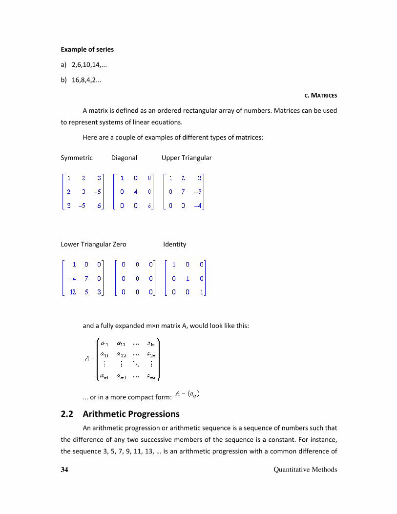
C. MATRICES
A matrix is defined as an ordered rectangular array of numbers. Matrices can be used
to represent systems of linear equations.
Here are a couple of examples of different types of matrices:
Symmetric Diagonal Upper Triangular
Lower Triangular Zero Identity
and a fully expanded m×n matrix A, would look like this:
... or in a more compact form:
2.2 Arithmetic Progressions
An arithmetic progression or arithmetic sequence is a sequence of numbers such that
the difference of any two successive members of the sequence is a constant. For instance,
the sequence 3, 5, 7, 9, 11, 13, … is an arithmetic progression with a common difference of

Quantitative Methods 35
2.
If the initial term of an arithmetic progression is a1 and the common difference of
successive members is d, then the nth term of the sequence is given by:
and in general
A finite portion of an arithmetic progression is called a finite arithmetic progression
and sometimes just called an arithmetic progression.
The behaviour of the arithmetic progression depends on the common difference d. If
the common difference is:
• Positive, the members (terms) will grow towards positive infinity.
• Negative, the members (terms) will grow towards negative infinity.
Examples:
Each one of the following series form an A.P.
• 1, 3, 5, 7…
• 3, 7, 11, 15…
• 15, 12, 9…
• x, x - d, x - 2d, .....
• a, a+d, a+2d, a+3d, a+4d…
The common difference is found by subtracting any term of the series from the
immediate succeeding term.
In the above example, common difference in the first is 2, in the second it is 4, in the
third it is -3, in the fourth it is -d and in the fifth it is d.
The general form of an A.P. is as follows:
a = first term, d = common difference, then A.P. is a, a+d, a+2d, a+3d,.....
In any term, the coefficient of d is less by one than the number of terms in the series.
Thus, second term is a+d
third term is a+2d

36 Quantitative Methods
fourth term is a+3d
tenth term is a+9d
and generally, nth
term is a + (n-1)d.
If n is the number of terms and if tn is the nth term, then
tn = a+(n-1)d.
2.2.1 SUM IN A.P.
The sum of the members of a finite arithmetic progression is called an arithmetic
series.
To find the sum of a number of terms in arithmetical progression:
Let a=first term, d=common difference, l=tn=last term, s=required sum. Then,
Writing the series in the reverse order,
Adding together the two series,
Expression i is used when the first term and the last term are given and the
expression ii is used when the first and the common difference are given. In any question
involving the five quantities a, d, l, n and s, we can determine all of them if any three are
given.
Remark
• If the same quantity is added to or subtracted from every term of an A.P, then the
resulting series will be an A.P. having the same common difference.

Quantitative Methods 37
• If every term of an A.P. is multiplied by the same quantity, the resulting series will be in
A.P.
• If every term of a series in A.P. is divided by the same quantity, the resulting series will
be an A.P.
• If three terms are given to be in A.P., it is convenient to take them as: a-d, a, a+d.
• If four terms are given to be in A.P, it is convenient to take them as:
a-3d, a-d,a+d,a+3d
• If five terms are given to be in A.P, it is convenient to take them as:
a-2d, a-d, a, a+d, a+2d
Example 2
Express the arithmetic series in two different ways:
Adding both sides of the two equations, all terms involving d cancel:
Rearranging and remembering that an = a1 + (n − 1)d:
So, for example, the sum of the terms of the arithmetic progression given by an = 3 +
(n-1)(5) up to the 50th term is
2.2.2 PRODUCT IN A.P.
The product of the members of a finite arithmetic progression with an initial element
a1, common differences d and n elements in total is determined in a closed expression by
where denotes the rising factorial and Γ denotes the gamma function. (Note,
however, that the formula is not valid when a1 / d is a negative integer or zero.)

38 Quantitative Methods
This is a generalisation from the fact that the product of the progression
is given by the factorial n! and that the product
for positive integers m and n is given by
Taking the example from above, the product of the terms of the arithmetic
progression given by an = 3 + (n-1)(5) up to the 50th term is
Study Notes
Assessment
1. Find the sum of the first 10 numbers from this arithmetic progression 1, 11, 21, 31.
2. Find the sum of the first 1000 odd numbers.
Discussion
Discuss sequence, series and matrices.

Quantitative Methods 39
2.3 Geometric Progressions
A geometric progression, also known as a geometric sequence, is a sequence of
numbers where each term after the first is found by multiplying the previous one by a fixed
non-zero number called the common ratio. For example, the sequence 2, 6, 18, 54, ... is a
geometric progression with a common ratio 3. Similarly 10, 5, 2.5, 1.25, ... is a geometric
sequence with a common ratio 1/2. The sum of the terms of a geometric progression is
known as a geometric series.
Thus, the general form of a geometric sequence is
and that of a geometric series is
where r ≠ 0 is the common ratio and a is a scale factor, equal to the sequence's start
value.
nth
term of the geometric progression is,
an=ar (n-1)
2.3.1 ELEMENTARY PROPERTIES OF G.P.
The n-th term of a geometric sequence with initial value a and common ratio r is
given by
Such a geometric sequence also follows the recursive relation
for every integer
Generally, to check whether a given sequence is geometric, one simply checks
whether all successive entries in the sequence have the same ratio.
The common ratio of a geometric series may be negative, resulting in an alternating
sequence with numbers switching from positive to negative and back. For instance,
1, −3, 9, −27, 81, −243, …
is a geometric sequence with a common ratio of −3.
The behaviour of a geometric sequence depends on the value of the common ratio.
If the common ratio is:

40 Quantitative Methods
• Positive, the terms will all be the same sign as the initial term.
• Negative, the terms will alternate between positive and negative.
• Greater than 1, there will be exponential growth towards positive infinity.
• 1, the progression is a constant sequence.
• Between −1 and 1 but not zero, there will be exponential decay towards zero.
• −1, the progression is an alternating sequence
• Less than −1, for the absolute values there is exponential growth towards positive and
negative infinity (due to the alternating sign).
Geometric sequences (with common ratio not equal to −1,1 or 0) show exponential
growth or exponential decay, as opposed to the linear growth (or decline) of an arithmetic
progression such as 4, 15, 26, 37, 48, … (with common difference 11). This result was taken
by T.R. Malthus as the mathematical foundation of his book Principle of Population. Note
that the two kinds of progression are related: exponentiation of each term in an arithmetic
progression yields a geometric progression, while taking the logarithm of each term in a
geometric progression with a positive common ratio yields an arithmetic progression.
2.3.2 GEOMETRIC SERIES
A geometric series is the sum of the numbers in a geometric progression:
We can find a simpler formula for this sum by multiplying both sides of the above
equation by 1 − r and we will see that
since all the other terms cancel. Rearranging (for r ≠ 1) gives the convenient formula
for a geometric series:
Quantitative Methods 41
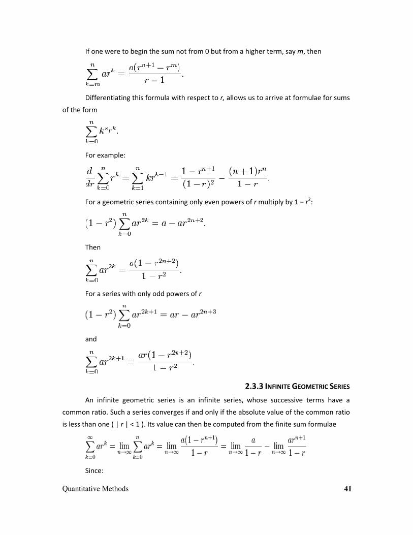
If one were to begin the sum not from 0 but from a higher term, say m, then
Differentiating this formula with respect to r, allows us to arrive at formulae for sums
of the form
For example:
For a geometric series containing only even powers of r multiply by 1 − r2:
Then
For a series with only odd powers of r
and
2.3.3 INFINITE GEOMETRIC SERIES
An infinite geometric series is an infinite series, whose successive terms have a
common ratio. Such a series converges if and only if the absolute value of the common ratio
is less than one ( | r | < 1 ). Its value can then be computed from the finite sum formulae
Since:

42 Quantitative Methods
Then:
For a series containing only even powers of r,
and for odd powers only,
In cases, where the sum does not start at k = 0,
The formulae given above are valid only for | r | < 1. The latter formula is valid in
every branch of algebra, as long as the norm of r is less than one and also in the field of p-
adic numbers if | r |p < 1. As in the case for a finite sum, we can differentiate to calculate
formulae for related sums. For example,
This formula only works for | r | < 1 as well. From this, it follows that, for | r | < 1,
Also, the infinite series 1/2 + 1/4 + 1/8 + 1/16 + · · · is an elementary example of a
series that converges absolutely.
It is a geometric series, whose first term is 1/2 and whose common ratio is 1/2, so its
sum is
The inverse of the above series is 1/2 − 1/4 + 1/8 − 1/16 + · · · is a simple example of
an alternating series that converges absolutely.

Quantitative Methods 43
It is a geometric series, whose first term is 1/2 and whose common ratio is −1/2, so
its sum is
2.3.4 COMPLEX NUMBERS
The summation formula for geometric series remains valid even when the common
ratio is a complex number. In this case, the condition that the absolute value of r be less
than 1 becomes that the modulus of r be less than 1. It is possible to calculate the sums of
some non-obvious geometric series. For example, consider the proposition
The proof of this comes from the fact that
which is a consequence of Euler's formula. Substituting this into the original series
gives
.
This is the difference of two geometric series and thus is a straightforward
application of the formula for infinite geometric series that completes the proof.
2.3.5 PRODUCT IN G.P.
The product of a geometric progression is the product of all the terms. If all the terms
are positive, then it can be quickly computed by taking the geometric mean of the
progression's first and last term and raising that mean to the power given by the number of
terms. (This is very similar to the formula for the sum of terms of an arithmetic sequence:
take the arithmetic mean of the first and last term and multiply it with the number of
terms.)
(if a,r > 0).

44 Quantitative Methods
Proof:
Let the product be represented by P:
.
Now, carrying out the multiplications, we conclude that
.
Applying the sum of arithmetic series, the expression will yield
.
.
We raise both sides to the second power:
.
Consequently,
and
,
which concludes the proof.
Example for Geometric Progression:
81, 27, 9... Find the nth term formula and the value of the fifth term from the given
sequence.
Solution: The common ratio to the base r = . The nth
term formula is,
an = 81( )n−1
=> an = 81 × ( )n−1
Therefore, fifth term is,
a5 = 81 × ( )5 −1
=> 81 × ( )4

Quantitative Methods 45
=> 81 × ( )
=> a5 = 1.
Study Notes
Assessment
Question
A piece of equipment cost a certain factory Rs. 600,000. If it depreciates in value, 15%
the first year, 13.5 % the next year, 12% the third year, and so on, what will be its value
at the end of 10 years, all percentages applying to the original cost?
(1) 2,00,000
(2) 1,05,000
(3) 4,05,000
(4) 6,50,000
[Hint: The total cost being Rs. 6,00,000/100 * 17.5 = Rs. 1,05,000.]
Discussion
Discuss difference between Arithmetic Progression and Geometric Progression.

46 Quantitative Methods
2.4 Harmonic Progression
A harmonic progression is a progression formed by taking the reciprocals of an
arithmetic progression. In other words, it is a sequence of the form
where −1/d is not a natural number. Equivalently, a sequence is a harmonic
progression when each term is the harmonic mean of the neighbouring terms.
Examples are:
12, 6, 4, 3, 12/5, 2, …
10, 30, −30, −10, −6, −30/7, …
2.4 1 HARMONIC SERIES
In mathematics, the harmonic series is the divergent infinite series:
Its name is derived from the concept of overtones or harmonics in music. For
example, the wavelengths of the overtones of a vibrating string are 1/2, 1/3, 1/4, etc of the
string's fundamental wavelength. Every term of the series after the first is the harmonic
mean of the neighbouring terms; the term harmonic mean likewise is derived from music.
The harmonic series is counterintuitive to students first encountering it because it is
a divergent series in spite of the fact that each of its terms tends to zero. Thus, an infinite
sum of numbers each of which has a value tending to zero might not be finite. The
divergence of the harmonic series is also the source of some apparent paradoxes or
counterintuitive results.
For example, one paradox is the "worm on the rubber band". Suppose that a worm
crawls along a 1 metre rubber band and after each minute, the rubber band is stretched by
an additional 1 metre. If the worm travels 1 centimetre per minute, will the worm ever reach
the end of the rubber band? The answer, counter intuitively, is "yes", for after n minutes,
the ratio of the distance travelled by the worm to the total length of the rubber band is
The series gets arbitrarily large as n becomes larger. Eventually, this ratio must

Quantitative Methods 47
exceed 1, which implies that the worm reaches the end of the rubber band. The value of n at
which this occurs must be extremely large; however, approximately e100: a number
exceeding 1040
(a one with 40 zeros after it). Although the harmonic series diverges, it
diverges very slowly.
Another example is that given a collection of identical dominoes, it is clearly possible
to stack them at the edge of a table, so that they hang over the edge of the table. The
counterintuitive result is that one can stack them in such a way as to make the overhang
arbitrarily large, provided there are enough dominoes.
2.4.2 DIVERGENCE
The harmonic series diverges to +∞. There are several well-known proofs of this fact.
• Comparison test
One way to prove divergence is to compare the harmonic series with another
divergent series:
Each term of the harmonic series is greater than or equal to the corresponding term
of the second series and therefore, the sum of the harmonic series must be greater than the
sum of the second series. However, the sum of the second series is infinite:
It follows (by the comparison test) that the sum of the harmonic series must be
infinite as well. More precisely, the comparison above proves that
for every positive integer k. This proof, due to Nicole Oresme, is a high point of
medieval mathematics. It is still a standard proof taught in mathematics classes today.
Cauchy's condensation test is a generalisation of this argument.
48 Quantitative Methods
• Integral test
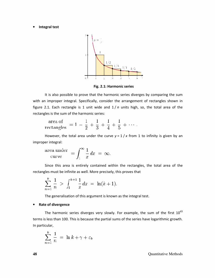
Fig. 2.1: Harmonic series
It is also possible to prove that the harmonic series diverges by comparing the sum
with an improper integral. Specifically, consider the arrangement of rectangles shown in
figure 2.1. Each rectangle is 1 unit wide and 1 / n units high, so, the total area of the
rectangles is the sum of the harmonic series:
However, the total area under the curve y = 1 / x from 1 to infinity is given by an
improper integral:
Since this area is entirely contained within the rectangles, the total area of the
rectangles must be infinite as well. More precisely, this proves that
The generalisation of this argument is known as the integral test.
• Rate of divergence
The harmonic series diverges very slowly. For example, the sum of the first 1043
terms is less than 100. This is because the partial sums of the series have logarithmic growth.
In particular,

Quantitative Methods 49
where γ is the Euler–Mascheroni constant and εk approaches 0 as k goes to infinity.
This result is due to Leonhard Euler.
2.4.3 PARTIAL SUMS
The nth partial sum of the diverging harmonic series,
is called the nth harmonic number.
The difference between the nth harmonic number and the natural logarithm of n
converges to the Euler-Mascheroni constant.
The difference between distinct harmonic numbers is never an integer.
No harmonic numbers are integers, except for n = 1.
Study Notes
Assessment
1. Does x=3, y=4, z=6 are in harmonic progression ? how to find that ?
2. How to find the mean of a harmonic progression ?
Discussion
Discuss how Harmonic Progression different from Geometric Progression?

50 Quantitative Methods
2.5 Managerial Application of Sequence and Series
Sequences and series, whether arithmetic or geometric, have many applications.
To work with these application problems, one needs to have a basic understanding of
arithmetic series, arithmetic sequences, harmonic series, harmonic sequences,
geometric sequences and geometric series.
For example,
i.) A theatre has 20 seats in the first row, 24 seats in the second row, 28 seats in
the third row and so on. It has 30 rows of seats in all. How many seats are there in the
theatre?
To solve this problem, we need to ask and answer some preliminary questions.
First, what is the problem asking us to do? We need to know how many seats
are there in the auditorium, which means that we are counting things and finding a
total. Also, we need to add up all the seats in each row. Since we are adding things up,
this can be looked at as a series. Although we have formulas for series problems, we
need to know if the problem is arithmetic or geometric so that we know which formula
to use.
To find out if the problem is arithmetic or geometric, look at the pattern in the
problem. There are 20 seats in the first row, 24 in the second row and 28 in the third
row. Each row has four more seats than the one before it. Since we are adding four to
each row, this is an arithmetic sequence of numbers that we will be adding up.
Thus, we now know that our goal is to find an arithmetic series. The formula for
an arithmetic series is
To solve this problem we need n, a1 and an. In this problem, n will be equal to 30
because we are being asked to find out how many seats are there in all 30 rows or to
add up the seats in the 30 rows. The first term in the sequence, a1, is 20 because the
problem tells us that the first row has 20 seats. The only thing left to do is to find an
which will be a30.
To find a30, we need the formula for the sequence and then we substitute n = 30.
The formula for an arithmetic sequence is
Quantitative Methods 51
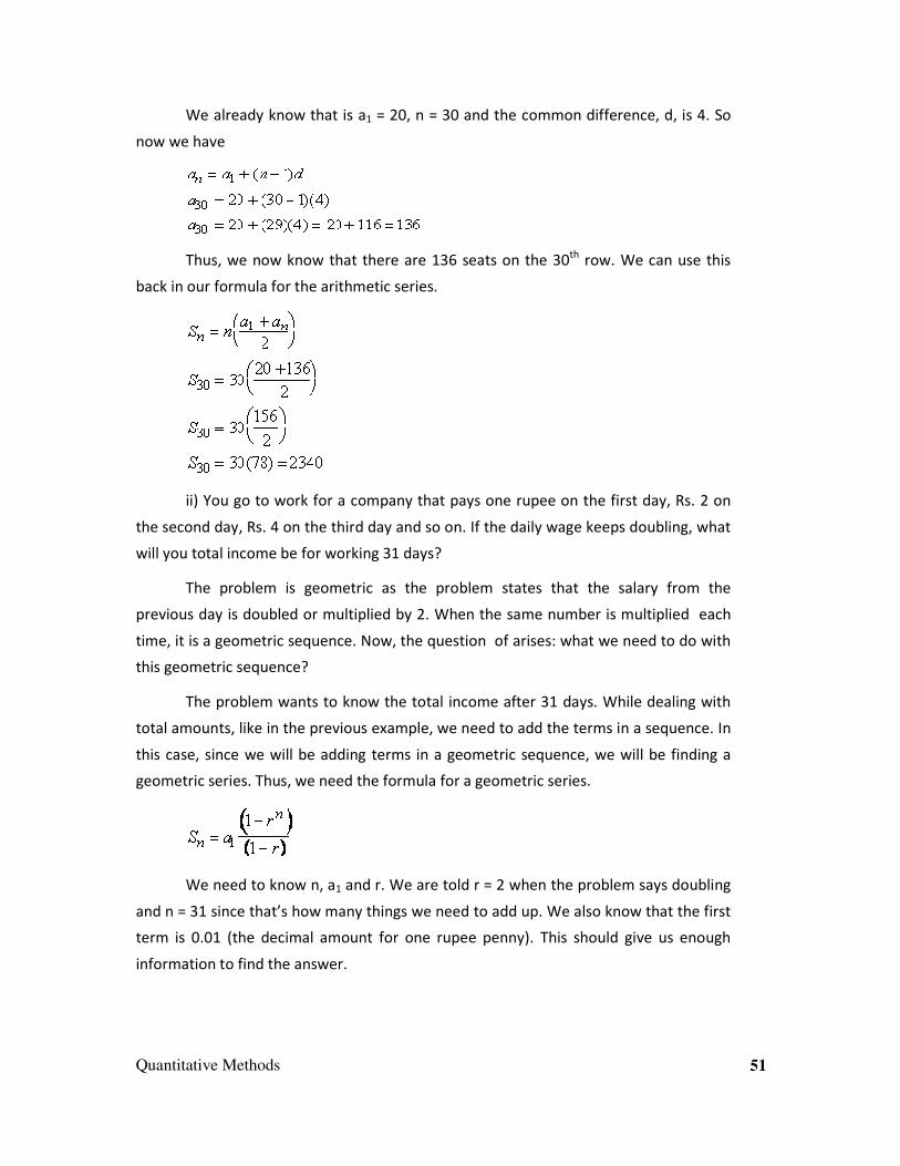
We already know that is a1 = 20, n = 30 and the common difference, d, is 4. So
now we have
Thus, we now know that there are 136 seats on the 30th row. We can use this
back in our formula for the arithmetic series.
ii) You go to work for a company that pays one rupee on the first day, Rs. 2 on
the second day, Rs. 4 on the third day and so on. If the daily wage keeps doubling, what
will you total income be for working 31 days?
The problem is geometric as the problem states that the salary from the
previous day is doubled or multiplied by 2. When the same number is multiplied each
time, it is a geometric sequence. Now, the question of arises: what we need to do with
this geometric sequence?
The problem wants to know the total income after 31 days. While dealing with
total amounts, like in the previous example, we need to add the terms in a sequence. In
this case, since we will be adding terms in a geometric sequence, we will be finding a
geometric series. Thus, we need the formula for a geometric series.
We need to know n, a1 and r. We are told r = 2 when the problem says doubling
and n = 31 since that’s how many things we need to add up. We also know that the first
term is 0.01 (the decimal amount for one rupee penny). This should give us enough
information to find the answer.

52 Quantitative Methods
More than Rs. 21.474 lakhs for 31 days work.
Practice Questions:
1. Logs are stacked in a pile with 24 logs on the bottom row and 15 on the top row.
There are 10 rows in all with each row having one more log than the one above it.
How many logs are in the stack?
2. Each hour, a grandfather clock chimes the number of times that corresponds to the
time of the day. For example, at 3:00, it will chime 3 times. How many times does
the clock chime in a day?
3. A ball is dropped from a height of 16 feet. Each time it drops, it rebounds to 80% of
the height from which it is falling. Find the total distance travelled in 15 bounces.
4. A company is offering a job with a salary of $30,000 for the first year and a 5% raise
each year after that. If that 5% raise continues every year, find the amount of
money you would earn in a 40-year career.
Study Notes

Quantitative Methods 53
Assessment
(a) Write the recurring decimal 0·474747….. as an infinite geometric series and
hence as a fraction.
(b) In an arithmetic sequence, the fifth term is –18 and the tenth term is 12.
(i) Find the first term and the common difference.
(ii) Find the sum of the first fifteen terms of the sequence.
Ans: (a) 47/99, (b) (i) a = –42, d = 6 (ii) S15 = 0
Discussion
Discuss application of A.P., G.P. and H.P. in real life.
2.6 Matrices
In mathematics, a matrix (plural matrices or less commonly matrixes) is a rectangular
array of numbers such as:
An item in a matrix is called an entry or an element. The example has entries 1, 9, 13,
20, 55 and 4. Entries are often denoted by a variable with two subscripts, as shown above.
Matrices of the same size can be added and subtracted entry-wise and matrices of
compatible sizes can be multiplied. These operations have many of the properties of
ordinary arithmetic, except that matrix multiplication is not commutative, i.e. AB and BA are
not equal in general. Matrices consisting of only one column or row define the components
of vectors, while higher-dimensional (e.g. three-dimensional) arrays of numbers define the
components of a generalisation of a vector called a tensor. Matrices with entries in other
fields or rings are also studied.
A major branch of numerical analysis is devoted to the development of efficient
algorithms for matrix computations, a subject that is centuries old but is still an active area
of research. Matrix decomposition methods simplify computations both, theoretically and
practically. For sparse matrices, specifically tailored algorithms can provide speedups. Such
matrices arise in the finite element method.

54 Quantitative Methods
Specific entries of a matrix are often referenced by using pairs of subscripts.
2.6.1 DEFINITION OF MATRICES
A matrix is a rectangular arrangement of numbers. For example,
An alternative notation uses large parentheses instead of box brackets:
The horizontal and vertical lines in a matrix are called rows and columns,
respectively. The numbers in the matrix are called its entries or its elements. To specify a
matrix's size, a matrix with m rows and n columns is called an m-by-n matrix or m × n matrix,
while m and n are called its dimensions. The matrix above is a 4-by-3 matrix.
A matrix with one row (a 1 × n matrix) is called a row vector and a matrix with one
column (an m × 1 matrix) is called a column vector. Any row or column of a matrix
determines a row or column vector, obtained by removing all other rows respectively
columns from the matrix. For example, the row vector for the third row of the above matrix
A is
When a row or column of a matrix is interpreted as a value, this refers to the
corresponding row or column vector. For instance, one may say that two different rows of a

Quantitative Methods 55
matrix are equal, meaning that they determine the same row vector. In some cases, the
value of a row or column should be interpreted as a sequence of values (an element of Rn if
entries are real numbers) rather than as a matrix, for instance, when saying that the rows of
a matrix are equal to the corresponding columns of its transpose matrix.
Most of this section focuses on real and complex matrices, i.e. matrices, whose
entries are real or complex numbers.
2.6.2 NOTATION
The specifics of matrices notation varies widely, with some prevailing trends.
Matrices are usually denoted using upper-case letters, while the corresponding lower-case
letters, with two subscript indices, represent the entries. In addition to using upper-case
letters to symbolise matrices, many authors use a special typographical style, commonly
boldface upright (non-italic), to further distinguish matrices from other variables. An
alternative notation involves the use of a double-underline with the variable name, with or
without boldface style. e.g. .
The entry that lies in the i-th row and the j-th column of a matrix is typically referred
to as the i,j, (i,j) or (i,j)th entry of the matrix. For example, the (2,3) entry of the above matrix
A is 7. The (i, j)th entry of a matrix A is most commonly written as ai,j. Alternative notations
for that entry are A[i,j] or Ai,j.
Sometimes, a matrix is referred to by giving a formula for its (i,j)th entry, often with
double parenthesis around the formula for the entry. For example, if the (i,j)th entry of A
were given by aij, A would be denoted ((aij)).
An asterisk is commonly used to refer to whole rows or columns in a matrix. For
example, ai,∗ refers to the ith row of A and a∗,j refers to the jth column of A. The set of all m-
by-n matrices is denoted (m, n).
A common shorthand is
A = [ai,j]i=1,...,m; j=1,...,n or more briefly A = [ai,j]m×n
to define an m × n matrix A. Usually the entries ai,j are defined separately for all
integers 1 ≤ i ≤ m and 1 ≤ j ≤ n. They can however, sometimes be given by one formula. For
example, the 3-by-4 matrix
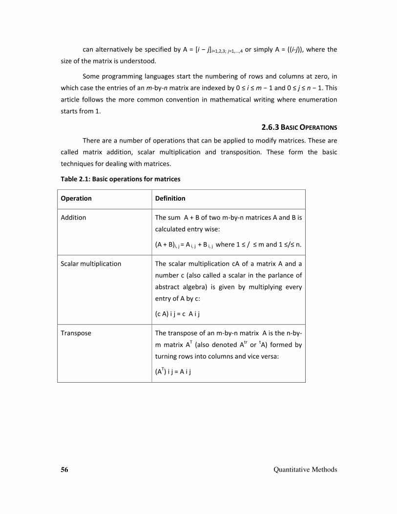
56 Quantitative Methods
can alternatively be specified by A = [i − j]i=1,2,3; j=1,...,4 or simply A = ((i-j)), where the
size of the matrix is understood.
Some programming languages start the numbering of rows and columns at zero, in
which case the entries of an m-by-n matrix are indexed by 0 ≤ i ≤ m − 1 and 0 ≤ j ≤ n − 1. This
article follows the more common convention in mathematical writing where enumeration
starts from 1.
2.6.3 BASIC OPERATIONS
There are a number of operations that can be applied to modify matrices. These are
called matrix addition, scalar multiplication and transposition. These form the basic
techniques for dealing with matrices.
Table 2.1: Basic operations for matrices
Operation Definition
Addition The sum A + B of two m-by-n matrices A and B is
calculated entry wise:
(A + B)i, j = A i, j + B i, j where 1 ≤ / ≤ m and 1 ≤/≤ n.
Scalar multiplication The scalar multiplication cA of a matrix A and a
number c (also called a scalar in the parlance of
abstract algebra) is given by multiplying every
entry of A by c:
(c A) i j = c A i j
Transpose The transpose of an m-by-n matrix A is the n-by-
m matrix AT (also denoted A
tr or
tA) formed by
turning rows into columns and vice versa:
(AT) i j = A i j

Quantitative Methods 57
Familiar properties of numbers extend to these operations of matrices: for example,
addition is commutative, i.e. the matrix sum does not depend on the order of the
summands: A + B = B + A. The transpose is compatible with addition and scalar
multiplication, as expressed by (cA)T = c(AT) and (A + B)T = AT + BT. Finally, (AT)T = A.
Row operations are ways to change matrices. There are three types of row
operations: row switching, i.e. is interchanging two rows of a matrix, row multiplication, i.e.
multiplying all entries of a row by a non-zero constant and finally row addition, which means
adding a multiple of a row to another row. These row operations are used in a number of
ways including solving linear equations and finding inverses.
2.6.4 MATRIX MULTIPLICATION
Fig. 2.2: Matrices Multiplication

58 Quantitative Methods
Schematic depiction of the matrix product AB of two matrices A and B.
Multiplication of two matrices is defined only if the number of columns of the left
matrix is the same as the number of rows of the right matrix. If A is an m-by-n matrix and B is
an n-by-p matrix, then their matrix product AB is the m-by-p matrix, whose entries are given
by dot-product of the corresponding row of A and the corresponding column of B:
where 1 ≤ i ≤ m and 1 ≤ j ≤ p. For example (the underlined entry 1 in the product is
calculated as the product 1 · 1 + 0 · 1 + 2 · 0 = 1):
Matrix multiplication satisfies the rules (AB)C = A(BC) (associativity) and (A+B)C =
AC+BC as well as C(A+B) = CA+CB (left and right distributivity), whenever the size of the
matrices is such that the various products are defined. The product AB may be defined
without BA being defined, namely if A and B are m-by-n and n-by-k matrices, respectively
and m ≠ k. Even if both products are defined, they need not be equal, i.e. generally one has
AB ≠ BA,
i.e. matrix multiplication is not commutative, in marked contrast to (rational, real or
complex) numbers, whose product is independent of the order of the factors. An example of
two matrices not commuting with each other is:
whereas
The identity matrix In of size n is the n-by-n matrix in which all the elements on the
main diagonal are equal to 1 and all other elements are equal to 0,
e.g.

Quantitative Methods 59
It is called identity matrix because multiplication with it leaves a matrix unchanged:
MIn = ImM = M for any m-by-n matrix M.
Besides, the ordinary matrix multiplication just described, there exists other less
frequently used operations on matrices that can be considered to be forms of multiplication.
This includes the Hadamard product and the Kronecker product. They arise in solving matrix
equations such as the Sylvester equation.
2.6.5 APPLICATION OF MATRICES
There are numerous applications of matrices, both in mathematics and other
sciences. Some of them merely take advantage of the compact representation of a set of
numbers in a matrix. For example, in Game Theory and economics, the payoff matrix
encodes the payoff for two players, depending on which out of a given (finite) set of
alternatives the players choose. Text mining and automated thesaurus compilation makes
use of document-term matrices such as tf-idf in order to keep track of frequencies of certain
words in several documents.
Matrices are a key tool in linear algebra. One use of matrices is to represent linear
transformations, which are higher-dimensional analogs of linear functions of the form f(x) =
cx, where c is a constant; matrix multiplication corresponds to composition of linear
transformations. Matrices can also keep track of the coefficients in a system of linear
equations. For a square matrix, the determinant and inverse matrix (when it exists) govern
the behaviour of solutions to the corresponding system of linear equations and Eigen values
and eigenvectors provide insight into the geometry of the associated linear transformation.
Matrices have many applications. Physics makes use of matrices in various domains,
for example, in geometrical optics and matrix mechanics; the latter led to detailed studying
of matrices with an infinite number of rows and columns. Graph theory uses matrices to
keep track of distances between pairs of vertices in a graph. Computer graphics uses
matrices to project 3-dimensional space onto a 2-dimensional screen. Matrix calculus
generalises classical analytical notions such as derivatives of functions or exponentials to
matrices. The latter is a recurring need in solving ordinary differential equations. Serialism
and dodecaphonism are musical movements of the 20th century that use a square
mathematical matrix to determine the pattern of music intervals.
Complex numbers can be represented by particular real 2-by-2 matrices via

60 Quantitative Methods
under which addition and multiplication of complex numbers and matrices
correspond to each other. For example, 2-by-2 rotation matrices represent the
multiplication with some complex number of absolute value 1, as illustrated above. A similar
interpretation is possible for quaternions.
Early encryption techniques like the Hill cipher also used matrices. However, due to
the linear nature of matrices, these codes are comparatively easy to break. Computer
graphics uses matrices both to represent objects and to calculate transformations of objects
using affine rotation matrices to accomplish tasks such as projecting a three-dimensional
object onto a two-dimensional screen, corresponding to a theoretical camera observation.
Matrices over a polynomial ring are important in the study of Control Theory.
Chemistry makes use of matrices in various ways, particularly since the use of the
Quantum Theory to discuss molecular bonding and spectroscopy. Examples are the overlap
matrix and the Fock matrix used in solving the Roothaan equations to obtain the molecular
orbitals of the Hartree–Fock method.
Study Notes

Quantitative Methods 61
Assessment
Tick the correct answer from the given choices:
1. What is the size of a Matrix,
?
a) 2 X 3
b) 3 X 2
c) 3 X 4
d) 4 X 3
2. What is entry (2,3) of the matrix,
?
a) 3
b) 4
c) 12
d) 14
3. What is the matrix 7Z if
Z = ?
a)
b)
c)
d)
4. Which of the following matrices is the identity matrix I4 ?

62 Quantitative Methods
a)
b)
c)
d)
Discussion
Discuss practical application of Matrices in daily life.
2.7 Markov Chains
A Markov chain is a random process with the property that the next state depends
only on the current state. It is a particular type of Markov process, named for Andrey
Markov, in which the process can only be in a finite or countable number of states. Markov
chains are useful as mathematical tools for statistical modelling in modern applied
mathematics, particularly in the information sciences.
2.7.1 CONCEPT OF MARKOV CHAINS
Formally, a Markov chain is a discrete random process with the Markov property.
Often, the term "Markov chain" is used to refer to a Markov process, which has a discrete
(finite or countable) state-space. Usually, a Markov chain would be defined for a discrete set
of times (i.e. a discrete-time Markov chain) although some authors use the same
terminology where "time" can take continuous values.
A "discrete-time" random process means a system, which is in a certain state at each
"step", with the state changing randomly between steps. The steps are often thought of as
time but they can equally well refer to physical distance or any other discrete measurement.
Formally, the steps are integers or natural numbers and the random process is a mapping of
these to states. The Markov property states that the conditional probability distribution for
the system at the next step (and in fact at all future steps) given its current state depends
only on the current state of the system and not additionally on the state of the system at
previous steps:

Quantitative Methods 63
Since the system changes randomly, it is generally impossible to predict the exact
state of the system in the future. However, the statistical properties of the system's future
can be predicted. In many applications, it is these statistical properties that are important.
The changes of state of the system are called transitions and the probabilities
associated with various state-changes are called transition probabilities. The set of all states
and transition probabilities completely characterises a Markov chain. By convention, we
assume that all possible states and transitions have been included in the definition of the
processes, thus there is always a next-state and the process goes on forever.
A famous Markov chain is the so-called "drunkard's walk", a random walk on the
number line where, at each step, the position may change by +1 or −1 with equal
probability. From any position, there are two possible transitions, either to the next or
previous integer. The transition probabilities depend only on the current position and not on
the way the position was reached. For example, the transition probabilities from 5 to 4 and 5
to 6 are both 0.5 and all other transition probabilities from 5 are 0. These probabilities are
independent of whether the system was previously in 4 or 6.
Another example is the dietary habits of a creature who eats only grapes, cheese or
lettuce and whose dietary habits conform to the following (artificial) rules: it eats exactly
once a day; if it ate cheese yesterday, it will not eat today and it will eat lettuce or grapes
with equal probability; if it ate grapes yesterday, it will eat grapes today with a probability of
1/10, cheese with a probability of 4/10 and lettuce with a probability of 5/10; finally, if it ate
lettuce yesterday, it won't eat lettuce again today but will eat grapes with a probability of
4/10 or cheese with a probability of 6/10. This creature's eating habits can be modelled with
a Markov chain since its choice depends on what it ate yesterday and not additionally on
what it ate 2 or 3 (or 4, etc) days ago. One statistical property one could calculate is the
expected percentage of the time for which the creature will eat grapes over a long period.
A series of independent events—for example, a series of coin flips—does satisfy the
formal definition of a Markov chain. However, the theory is usually applied only when the
probability distribution of the next step depends non-trivially on the current state.
Many other examples of Markov chains exist.
2.7.2 DEFINITION OF MARKOV CHAINS
A Markov chain is a sequence of random variables X1, X2, X3, ... with the Markov
property, namely that, given the present state, the future and past states are independent.

64 Quantitative Methods
Formally,
The possible values of Xi form a countable set S called the state space of the chain.
Markov chains are often described by a directed graph, where the edges are labelled
by the probabilities of going from one state to the other states.
2.7.3 VARIATIONS
• Continuous-time Markov processes have a continuous index.
• Time-homogeneous Markov chains (or stationary Markov chains) are processes where
for all n. The probability of the transition is independent of n.
• A Markov chain of order m (or a Markov chain with memory m) where m is finite, is a
process satisfying
In other words, the future state depends on the past m states. It is possible to
construct a chain (Yn) from (Xn) which has the 'classical' Markov property as follows:
Let Yn = (Xn, Xn−1, ..., Xn−m+1), the ordered m-tuple of X values. Then Yn is a Markov
chain with state space Sm and has the classical Markov property.
• An additive Markov chain of order m where m is finite, is where
for n > m.

Quantitative Methods 65
Example
Fig. 2.3: Markov chain
A simple example is shown in figure 2.3, using a directed graph to picture the state
transitions. The states represent whether the economy is in a bull market, a bear market or
recession, during a given week. According to the figure, a bull week is followed by another
bull week 90% of the time, a bear market 7.5% of the time and a recession the other 2.5%.
From this figure, it is possible to calculate, for example, the long-term fraction of time during
which the economy is in recession or on average how long it will take to go from recession
to a bull market.
A finite state machine can be used as a representation of a Markov chain. Assuming a
sequence of independent and identically distributed input signals (for example, symbols
from a binary alphabet chosen by coin tosses), if the machine is in state y at time n, then the
probability that it moves to state x at time n + 1 depends only on the current state.
2.7.4 REVERSIBLE MARKOV CHAIN
A Markov chain is said to be reversible if there is a π such that
This condition is also known as the detailed balance condition.
Summing over i gives
Thus, for reversible Markov chains, π is always a stationary distribution.
The idea of a reversible Markov chain comes from the ability to "invert" a conditional

66 Quantitative Methods
probability using Bayes' Rule:
Then, given the reversibility condition,
It now appears as if time has been reversed.
2.7.5 APPLICATION OF MARKOV CHAINS
Markov chains are applied in a number of ways to many different fields. Often, they
are used as a mathematical model from some random physical process; if the parameters of
the chain are known, quantitative predictions can be made. In other cases, they are used to
model a more abstract process and are the theoretical underpinning of an algorithm.
Testing: Several theorists have proposed the idea of the Markov chain statistical test
(MCST). This is a method of conjoining Markov chains to form a "Markov blanket", arranging
these chains in several recursive layers ("wafering") and producing more efficient test sets—
samples—as a replacement for exhaustive testing. MCSTs also have uses in temporal state-
based networks.
Information Sciences: Markov chains are used throughout information processing.
Claude Shannon's famous 1948 paper, A Mathematical Theory Of Communication, which in
a single step created the field of information theory, opens by introducing the concept of
entropy through Markov's modelling of the English language. Such idealised models can
capture many of the statistical regularities of systems. Even without describing the full
structure of the system perfectly, such signal models can make very effective data
compression possible through the entropy encoding technique of arithmetic coding. They
also allow effective state estimation and pattern recognition.
Markov chains are also the basis for Hidden Markov Models, which are an important
tool in such diverse fields as telephone networks (for error correction), speech recognition
and bioinformatics. The world's mobile telephone systems depend on the Viterbi algorithm
for error-correction, while hidden Markov models are extensively used in speech recognition
and also in bioinformatics, for instance, for coding region/gene prediction. Markov chains

Quantitative Methods 67
also play an important role in reinforcement learning.
Queuing Theory: Markov chains are the basis for the analytical treatment of queues
(Queuing Theory). This makes them critical for optimising the performance of
telecommunication networks where messages must often compete for limited resources
(such as bandwidth).
Internet Applications: The Page Rank of a webpage as used by Google is defined by a
Markov chain. It is the probability to be at page i in the stationary distribution on the
following Markov chain on all (known) WebPages. If N is the number of known webpages
and a page i has ki links then it has transition probability for all pages that are
linked to and for all pages that are not linked to. The parameter α is taken to be
about 0.85.
Markov models have also been used to analyse web navigation behaviour of users. A
user's web link transition on a particular website can be modelled using first- or second-
order Markov models and can be used to make predictions regarding future navigation and
to personalise the web page for an individual user.
Statistics: Markov chain methods have also become very important for generating
sequences of random numbers to accurately reflect very complicated desired probability
distributions, via a process called Markov chain Monte Carlo (MCMC). In recent years, this
has revolutionised the practicability of Bayesian inference methods, allowing a wide range of
posterior distributions to be simulated and their parameters found numerically.
Economics and Finance: Markov chains are used in Finance and Economics to model
a variety of different phenomena, including asset prices and market crashes. The first
financial model to use a Markov chain was from Prasad et al in 1974. Another was the
regime-switching model of James D. Hamilton (1989), in which a Markov chain is used to
model switches between periods of high volatility and low volatility of asset returns. A more
recent example is the Markov Switching Multifractal Asset Pricing Model, which builds upon
the convenience of earlier regime-switching models. It uses an arbitrarily large Markov chain
to drive the level of volatility of asset returns.
Dynamic macroeconomics is greatly dependent on Markov chains. An example is
using Markov chains to exogenously model prices of equity (stock) in a general equilibrium
setting.
Social Sciences: Markov chains are generally used in describing path-dependent

68 Quantitative Methods
arguments, where current structural configurations condition future outcomes. An example
is the commonly argued link between economic development and the rise of capitalism.
Once a country reaches a specific level of economic development, the configuration of
structural factors, such as size of the commercial bourgeoisie, the ratio of urban to rural
residence, the rate of political mobilization, etc., will generate a higher probability of
transitioning from authoritarian to capitalist.
Mathematical Biology: Markov chains also have many applications in biological
modelling, particularly population processes, which are useful in modelling processes that
are (at least) analogous to biological populations. The Leslie matrix is one such example,
though some of its entries are not probabilities (they may be greater than 1). Another
example is the modelling of a cell's shape in dividing sheets of epithelial cells. Yet another
example is the state of i in cell membranes.
Markov chains are also used in simulations of brain function such as the simulation of
the mammalian neocortex.
Study Notes
Assessment
1. A math teacher, not wanting to be predictable, decided to assign homework based on
probabilities. On the first day of class, she drew this picture on the board to tell the
students whether to expect a full assignment, a partial assignment, or no assignment
the next day.

Quantitative Methods 69
a. Construct and label the transition matrix that corresponds to this drawing. Label it A.
b. If students have a full assignment today, what is the probability that they will have a full
assignment again tomorrow?
c. If students have no assignment today, what is the probability that they will have no
assignment again tomorrow?
d. Today is Wednesday and students have a partial assignment. What is the probability
that they will have no homework on Friday?
e. Matrix A is the transition matrix for one day. Find the transition matrix for two days (for
example, if today is Monday, what are the chances of getting each kind of assignment
on Wednesday?).
f. Find the transition matrix for three days.
g. If you have no homework this Friday, what is the is the probability that you will have no
homework next Friday (since we are only considering school days, there are only 5 days
in a week)? Give your answer accurate to two decimal places.
h. Find, to two decimal places, the matrix to which matrix A would appear to converge
after many days.
i. Explain the meaning of your solution to problem 7h.
Answers
a.
The students might arrange the rows and, therefore the columns, in a different order.

70 Quantitative Methods
b. 0.4
c. 0.05
d. 0.18
e.
f.
g. 0.18
h.
i. If we are looking far enough into the future (a few weeks or longer), it doesn't
matter what kind of assignment we have today. We have a 49% chance of having a full
assignment, a 33% chance of having a partial assignment and an 18% chance of not having
an assignment.
Discussion
Discuss application of Markov Chains.
2.8 Summary
Sequence: A set of numbers arranged in a definite order according to some definite
rule is called a sequence.
Series: A series is the sum of the terms of a sequence.
Arithmetic Progression: An arithmetic progression or arithmetic sequence is a
sequence of numbers such that the difference of any two successive members of the
sequence is a constant.

Quantitative Methods 71
Geometric Progression: A geometric progression, also known as a geometric
sequence, is a sequence of numbers where each term after the first is found by multiplying
the previous one by a fixed non-zero number called the common ratio.
Harmonic Progression: A harmonic progression is a progression formed by taking the
reciprocals of an arithmetic progression.
Matrix: A matrix is a rectangular arrangement of numbers.
The horizontal and vertical lines in a matrix are called rows and columns,
respectively. The numbers in the matrix are called its entries or its elements.
Markov Chains: A Markov chain is a random process with the property that the next
state depends only on the current state. It is a particular type of Markov process, named for
Andrey Markov, in which the process can only be in a finite or countable number of states.
2.9 Self Assessment Test
Exercises:
1. Find the sum of the first 10 numbers from this arithmetic progression 1, 11, 21, 31...
Solution: we can use this formula S = 1/2(2a1 + d(n-1))n
S = 1/2(2.1 + 10(10-1))10 = 5(2 + 90) = 5.92 = 460
2. Find the 5th term of the G.P 64, 16, 4... (Solution: 5th term of the given G.P is 1/4)
3. Matrices, A, B and C are given by
A = , B = and C =
If D = A(2B + 3C) find d23
Choose from the options given below:
• -56
• -109
• 19
• 324
72 Quantitative Methods
• 217
Short Notes
a. Arithmetic progression
b. Managerial applications of sequence and series
c. Matrix and its application in business
d. Markov chains and its applications
e. Sequences and series
2.10 Further Reading
1. Business Statistics by Examples, Terry, Sineich, Collier MacMillan Publishers, 1990
2. Basic Statistics for Management, Kazmier, L. J. and Pohl N. F., Prentice Hall Inc., 1995
3. Business Statistics, Gupta, S P and Gupta M P, New Delhi, Sultan Chand, 1997
4. Statistics for Behaviour and Social Scientists, Chadha, N. K., Reliance Publishing House,
1996
5. Statistics for Management, Levin Richard I. and Rubin David S, Prentice Hall Inc, 1995
6. Linear Programming and Decision Making, Narang, A.S., 1995

Quantitative Methods 73
Assignment
Write down examples from day-to-day life where matrix can be used.
___________________________________________________________________________
___________________________________________________________________________
___________________________________________________________________________
___________________________________________________________________________
___________________________________________________________________________
___________________________________________________________________________
___________________________________________________________________________
___________________________________________________________________________
___________________________________________________________________________
___________________________________________________________________________
___________________________________________________________________________
___________________________________________________________________________
___________________________________________________________________________
___________________________________________________________________________
___________________________________________________________________________
___________________________________________________________________________
___________________________________________________________________________
___________________________________________________________________________
___________________________________________________________________________
___________________________________________________________________________
___________________________________________________________________________
___________________________________________________________________________
___________________________________________________________________________

74 Quantitative Methods
___________________________________________________________________________
___________________________________________________________________________
___________________________________________________________________________
___________________________________________________________________________
___________________________________________________________________________
___________________________________________________________________________
___________________________________________________________________________
___________________________________________________________________________
___________________________________________________________________________
___________________________________________________________________________
___________________________________________________________________________
___________________________________________________________________________
___________________________________________________________________________
___________________________________________________________________________
___________________________________________________________________________
___________________________________________________________________________
___________________________________________________________________________
___________________________________________________________________________
___________________________________________________________________________
___________________________________________________________________________
___________________________________________________________________________
___________________________________________________________________________
___________________________________________________________________________
___________________________________________________________________________
___________________________________________________________________________

Quantitative Methods 75
Unit 3 Frequency and Probability Distribution
Learning Outcome
After reading this unit, you will be able to:
• Construct frequency distribution table
• Apply the table to frequency distribution-concept
• Explain probability theory and Probability distribution
• Identify Binomial and Poisson distribution
• Describe normal and exponential distribution
Time Required to Complete the unit
1. 1st
Reading: It will need 3 Hrs for reading a unit
2. 2nd Reading with understanding: It will need 4 Hrs for reading and understanding a
unit
3. Self Assessment: It will need 3 Hrs for reading and understanding a unit
4. Assignment: It will need 2 Hrs for completing an assignment
5. Revision and Further Reading: It is a continuous process
Content Map
3.1 Introduction
3.2 Frequency Distribution
3.2.1 Constructing Frequency Distribution Table
3.2.2 Class, Class Limits, Class Boundaries
3.2.3 General Rules for construction of Frequency Distribution
3.2.4 Uni-variate Frequency Tables

76 Quantitative Methods
3.2.5 Joint Frequency Distributions
3.2.6 Applications of Frequency Distribution
3.3 Introduction to Probability
3.3.1 Probability Theory
3.4 Probability Distributions
3.4.1 Definition of Probability Distribution
3.4.2 Discrete Probability Distribution
3.4.3 Continuous Probability Distribution
3.4.4 Bayes' Theorem
3.5 Binomial Distribution
3.5.1 Properties of Binomial Distribution
3.5.2 Binomial Distribution Formula
3.5.3 Examples
3.5.4 Cumulative Binomial Property
3.6 Poisson Distribution
3.6.1 Properties of Poisson Distribution
3.6.2 Formula of Poisson Distribution
3.6.3 Example Problems
3.7 Normal Distribution
3.7.1 Definition of Normal Distribution
3.7.2 Equation of Normal Distribution
3.7.3 Properties of Normal Distribution
3.7.4 Normal Variable and Normal Curve
3.7.5 The Standard Normal Distribution
3.7.6 The Z-Table
3.8 Exponential Distribution
3.8.1 Properties of Exponential Distribution

Quantitative Methods 77
3.8.2 Occurrence and Applications
3.9 Summary
3.10 Self Assessment Test
3.11 Further Reading

78 Quantitative Methods
3.1 Introduction
Numerical facts or measurements obtained in the course of an enquiry into a
phenomenon that has been marked by uncertainty, constitute statistical data. Statistical
data may be already available or may have to be collected by an investigator or an agency.
Data collected for the first time by the investigator (or on his behalf) is termed primary,
while data taken from records or data already available is termed as secondary. The
Meteorological Department regularly collects data on different aspects of weather and
climate such as amount of rainfall, humidity, maximum and minimum temperature of a
certain place. This is an example of primary data. To someone using this data for a certain
investigation afterwards, the data will be secondary.
The most important method of organising and summarising statistical data is by
constructing a distribution table. In this method, classification is done according to
quantitative magnitude. The items are classified into groups of classes according to their
increasing or decreasing order of magnitude and the number of items falling into each group
is determined and indicated.
In the science of statistics, we are not concerned about the occurrence of a single
event. The statement 'Stormy coast today' is the subject matter of the level of confidence
of the one who made it. On the other hand, in the subject field of statistics, the probability
where the generalised situation is defined is very useful for it.
The probability or chance for any comment or event will be judged on the basis of all
possible cases in which it may be true or other alternate possibilities when it may be false.
The concept of probability can be elaborated by means of two approaches viz,
mathematical approach and experimental approach. The mathematical approach concerns
the classical or Priori probability, which indicates that if an event can happen in p way and
fails to happen in q way, where the chances of occurrence of p and q are same, then the
probability of happening of p will be [p / (p+q)] and that of q will be [q / (p+q)]. This is also
called Laplace’s first Principle of probability.
In the second case, the experimental approach of probability, which is also known as
statistical or empirical probability, concerns the situation where the trial is repeated for a
large number of times under identical condition. Thus, in N trials, the event E happens t
times then the probability of happening E will be equal to that of (t/N) where N ranges up to
the infinity.
As a mathematical foundation for statistics, probability theory is essential to many
human activities that involve quantitative analysis of large sets of data. Methods of

Quantitative Methods 79
probability theory also apply to descriptions of complex systems given only partial
knowledge of their state, as in statistical mechanics. An important discovery of twentieth
century physics was the probabilistic nature of the physical phenomena at atomic scales,
described in quantum mechanics.
Most introductions to probability theory treat discrete probability distributions and
continuous probability distributions separately. The more mathematically advanced
Measure Theory-based treatment of probability covers both the discrete, the continuous,
any mix of these two and more.
3.2 Frequency Distribution
In statistics, a frequency distribution is a tabulation of the values that one or more
variables take in a sample. Each entry in the table contains the frequency or count of the
occurrences of values within a particular group or interval. In this way, the table summarises
the distribution of values in the sample.
3.2.1 CONSTRUCTING FREQUENCY DISTRIBUTION TABLE
Example 1: We consider here how a frequency distribution table is to be constructed
in the case of a discrete variable by taking a particular example.
Suppose the marks secured by 60 students of a class are as follows:
46, 57, 23,5,12 53, 38,58,26,43
36, 63,26,48,76 45, 66,74,16,86
56, 31,58,90,32 43, 36,66,46,58
36, 59,54,48,21 36, 64,58,45,76
58, 84,68,65,59 74, 48,64,58,50
46, 53,64,57,65 58, 95,56,66,44
Construct a Frequency Distribution Table
Marks obtained are divided into 10 groups or intervals as follows:
There are marks up to 10, between 11 and 20, between 11 and 30 and so on till
between 91 and 100. Represent each mark by a tally (/), for example, corresponding to the
mark 46 we put a tally (/) in the group 41 to 50: similarly, we continue putting tallies for
each mark. We continue up to four tallies and the fifth tally is put crosswise (\) so that it
becomes clear at once that the lot contains five tallies, i.e. there are five marks in that
group. A gap is left after a lot of five tallies, before starting again to mark tallies after each

80 Quantitative Methods
lot. The number of tallies in a class or group indicates the number of marks falling under that
group. This number is known as the frequency of that group or corresponding to that class
interval. Proceeding in this way, we get the following frequency table.
Table 3.1: Frequency Distribution of Marks Secured by 60 students
Class interval Tally
Frequency (No. of
students securing marks
which fall in the class
interval)
0 to 10 / 1
11 to 20 // 2
21 to 30 //// 4
31 to 40 //// // 7
41 to 50 //// //// // 12
51 to 60 //// //// //// 15
61 to 70 //// //// / 11
71 to 80 //// 4
81 to 90 /// 3
91 and above / 1
Total 60
We shall now consider construction of a frequency distribution table of a continuous
variable.
Example 2: The heights of 50 students to the nearest centimetre are given below:
151.1, 147.2, 145.3, 153.4, 156.5, 152.1, 159.2, 153.3, 157.4, 152.5,
144.1, 151.2, 157.3, 147.4, 150.5, 157.1, 153.2, 151.3, 149.4, 147.5,
151.1, 147.2, 155.3, 156.4, 151.5, 158.1, 149.2, 147.3, 153.4, 152.5,
149.1, 151.2, 153.3, 150.4, 152.5, 154.1, 150.2, 152.3, 149.4, 151.5,

Quantitative Methods 81
151.1, 154.2, 155.3, 152.4, 154.5, 152.1, 156.2, 155.3, 154.4, 150.5,
Construct a Frequency Distribution Table:
We have given heights in cms. In whole numbers, heights have been recorded to the
nearest centimetre. Thus a height of 144.50 or more but less than 145.5 is recorded as 145;
a height of 145.5 or more but less than 146.5 is recorded as 146 and so on. So the class 145-
146 could also be indicated by 144.5-146.5 implying the class which includes any height
greater than or equal to 144.5 but less than 145.5; the class 147-148 could be indicated by
146.5-148.5, meaning that the class which includes any height greater than or equal to 146.5
but less than 148.5. Following this convention, the classes could be represented as: 144.5-
146.5, 146.5-148.5 and so on. The above frequency distribution should thus be represented
as follows:
Table 3.2: Frequency distribution of heights of 50 students
Height Frequency (Number of students)
144.5-146.5 2
146.5-148.5 5
148.5-150.5 8
150.5-152.5 15
152.5-154.5 9
154.5-156.5 6
156.5-158.5 4
158.5-160.5 1
Total 50
3.2.2 CLASS, CLASS LIMITS, CLASS BOUNDARIES
The interval defining a class is known as a class interval. For Table 3.2, 145-146, 147-
148... are class intervals. The end numbers 145 and 146 of the class interval 145-146 are
known as class limits; the smaller number 145 is the lower class limit and larger number 146
is the upper class limit.
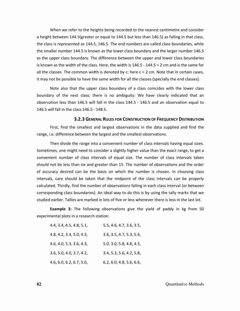
82 Quantitative Methods
When we refer to the heights being recorded to the nearest centimetre and consider
a height between 144.5(greater or equal to 144.5 but less than 146.5) as falling in that class,
the class is represented as 144.5, 146.5. The end numbers are called class boundaries, while
the smaller number 144.5 is known as the lower class boundary and the larger number 146.5
as the upper class boundary. The difference between the upper and lower class boundaries
is known as the width of the class. Here, the width is 146.5 - 144.5 = 2 cm and is the same for
all the classes. The common width is denoted by c: here c = 2 cm. Note that in certain cases,
it may not be possible to have the same width for all the classes (specially the end classes).
Note also that the upper class boundary of a class coincides with the lower class
boundary of the next class; there is no ambiguity: We have clearly indicated that an
observation less than 146.5 will fall in the class 144.5 - 146.5 and an observation equal to
146.5 will fall in the class 146.5 - 148.5.
3.2.3 GENERAL RULES FOR CONSTRUCTION OF FREQUENCY DISTRIBUTION
First, find the smallest and largest observations in the data supplied and find the
range, i.e. difference between the largest and the smallest observations.
Then divide the range into a convenient number of class intervals having equal sizes.
Sometimes, one might need to consider a slightly higher value than the exact range, to get a
convenient number of class intervals of equal size. The number of class intervals taken
should not be less than six and greater than 15. The number of observations and the order
of accuracy desired can be the basis on which the number is chosen. In choosing class
intervals, care should be taken that the midpoint of the class intervals can be properly
calculated. Thirdly, find the number of observations falling in each class interval (or between
corresponding class boundaries). An ideal way to do this is by using the tally marks that we
studied earlier. Tallies are marked in lots of five or less whenever there is less in the last lot.
Example 3: The following observations give the yield of paddy in kg from 50
experimental plots in a research station:
4.4, 3.4, 4.5, 4.8, 5.1, 5.5, 4.6, 4.7, 3.6, 3.5,
4.8, 4.2, 3.4, 5.0, 4.3, 3.6, 3.5, 4.7, 5.3, 5.4,
4.6, 4.0, 5.3, 3.6, 4.3, 5.0, 3.0, 5.8, 4.8, 4.5,
3.6, 5.0, 4.0, 3.7, 4.2, 3.4, 5.3, 5.6, 4.2, 5.8,
4.6, 6.0, 6.2, 6.7, 5.0, 6.2, 6.0, 4.8, 5.6, 6.6,

Quantitative Methods 83
Form a Frequency Distribution Table
Here, since the smallest observation is 3.0 and the largest is 6.7, the range is 6.7 - 3.0
= 3.7. Since there are 50 observations, we make each class of size 5 as follows: 2.9 - 3.4; 3.5 -
3.9 and so on. Taking the class size or width as 0.5, we can make 8 classes as 2.9 - 3.4; 3.5 -
3.9 and so on. The class limits for the class 3.0 -3.4 are 3.0 and 3.4. The class boundaries are
2.9 and 9.4 and so on. The width of a class
c = 3.4 - 2.9 = 0.5
Any observation between 2.9 and 3.4 will fall in the first class and weights are given
to the first decimal point. We now get the following frequency table:
Table 3.3: Distribution of Yield of Paddy in 50 Experimental Plots
Class interval Tally Frequency
2.9-3.4 //// 4
3.4-3.9 //// // 7
3.9-4.4 //// /// 8
4.4-4.9 //// //// / 11
4.9-5.4 //// //// 9
5.4-5.9 //// 5
5.9-6.4 //// 4
6.4-6.9 // 2
Total 50
3.2.4 UNI-VARIATE FREQUENCY TABLES
Univariate frequency distributions are often presented as lists ordered by the
quantity showing the number of times each value appears. For example, if 100 people rate a
five-point Likert scale assessing their agreement with a statement on a scale on which 1
denotes strong agreement and 5 strong disagreement, the frequency distribution of their
responses might look like:
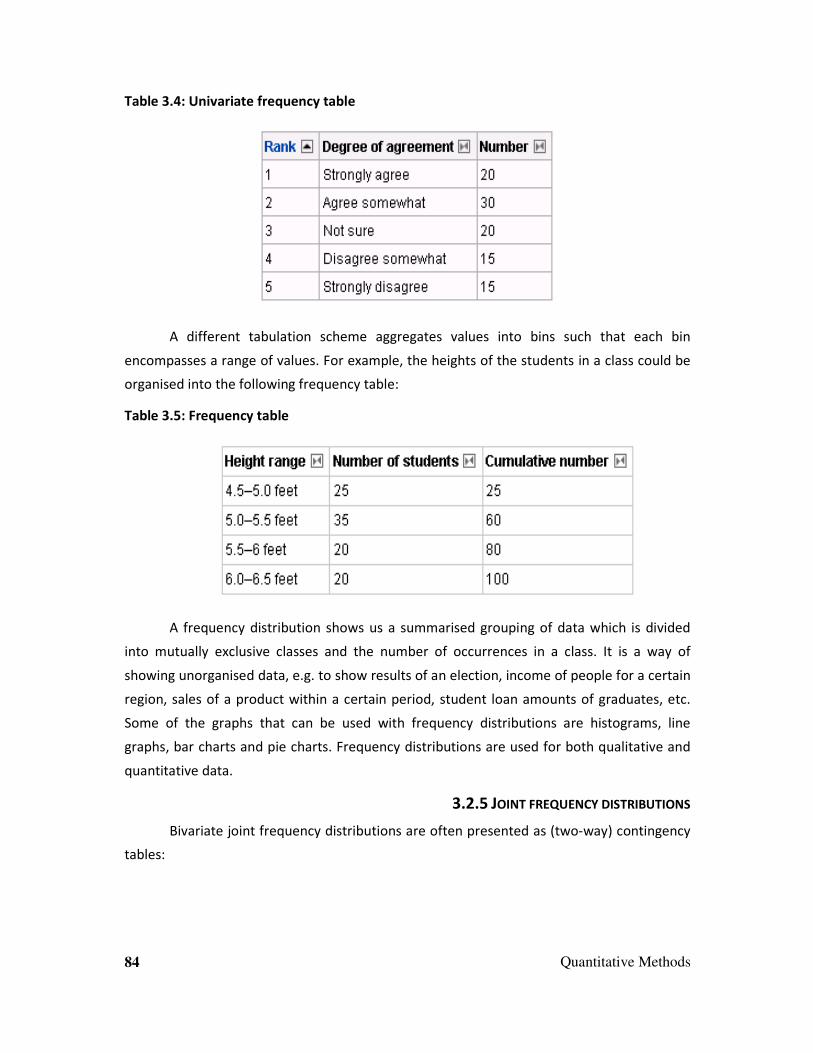
84 Quantitative Methods
Table 3.4: Univariate frequency table
A different tabulation scheme aggregates values into bins such that each bin
encompasses a range of values. For example, the heights of the students in a class could be
organised into the following frequency table:
Table 3.5: Frequency table
A frequency distribution shows us a summarised grouping of data which is divided
into mutually exclusive classes and the number of occurrences in a class. It is a way of
showing unorganised data, e.g. to show results of an election, income of people for a certain
region, sales of a product within a certain period, student loan amounts of graduates, etc.
Some of the graphs that can be used with frequency distributions are histograms, line
graphs, bar charts and pie charts. Frequency distributions are used for both qualitative and
quantitative data.
3.2.5 JOINT FREQUENCY DISTRIBUTIONS
Bivariate joint frequency distributions are often presented as (two-way) contingency
tables:
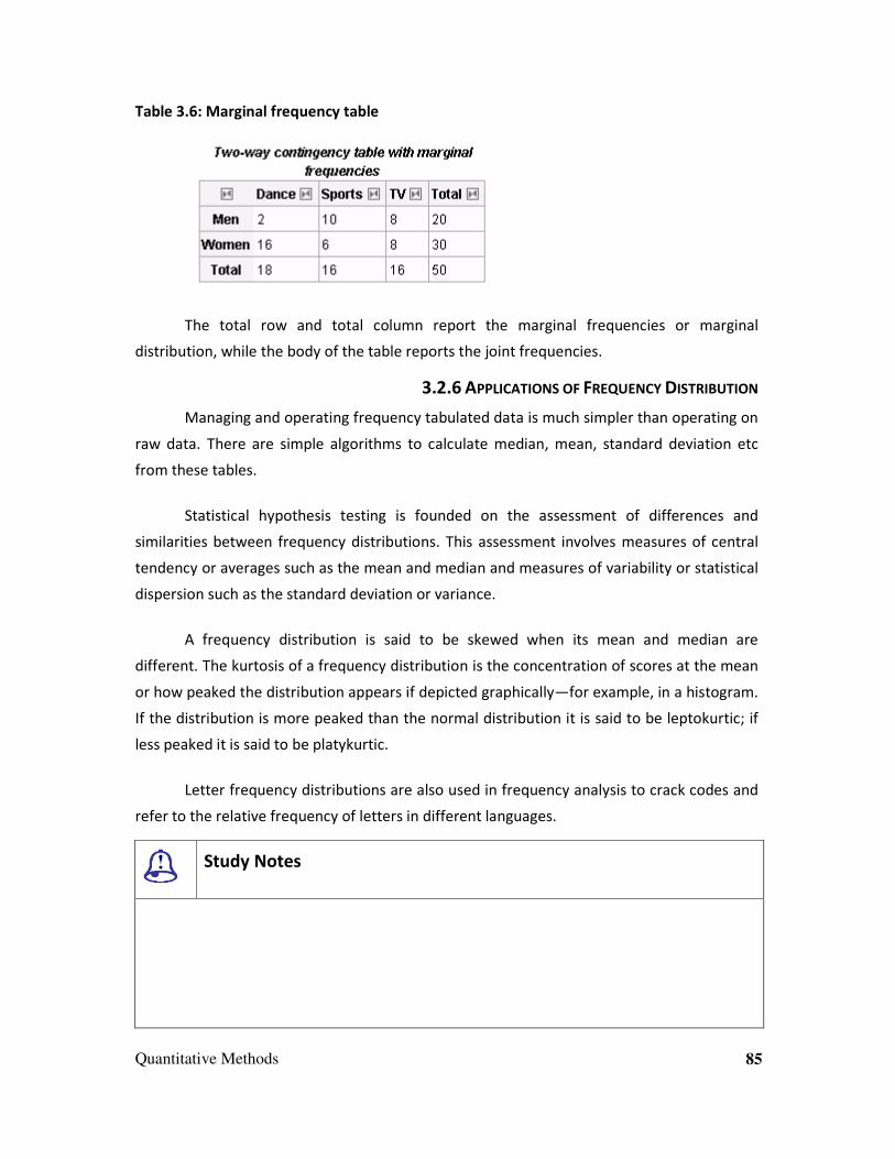
Quantitative Methods 85
Table 3.6: Marginal frequency table
The total row and total column report the marginal frequencies or marginal
distribution, while the body of the table reports the joint frequencies.
3.2.6 APPLICATIONS OF FREQUENCY DISTRIBUTION
Managing and operating frequency tabulated data is much simpler than operating on
raw data. There are simple algorithms to calculate median, mean, standard deviation etc
from these tables.
Statistical hypothesis testing is founded on the assessment of differences and
similarities between frequency distributions. This assessment involves measures of central
tendency or averages such as the mean and median and measures of variability or statistical
dispersion such as the standard deviation or variance.
A frequency distribution is said to be skewed when its mean and median are
different. The kurtosis of a frequency distribution is the concentration of scores at the mean
or how peaked the distribution appears if depicted graphically—for example, in a histogram.
If the distribution is more peaked than the normal distribution it is said to be leptokurtic; if
less peaked it is said to be platykurtic.
Letter frequency distributions are also used in frequency analysis to crack codes and
refer to the relative frequency of letters in different languages.
Study Notes

86 Quantitative Methods
Assessment
In the US Open Tennis 2002, Max Mirnyi played 5 matches, Andy Roddick played 5
matches, Kenneth Carlsen played 2 matches, Andre Agassi played 7 matches and Pete
Sampras played 6 matches. Pick an appropriate frequency table for the data.
Answer: (a) Table 1, (b) Table 2 (c) Table 3 (4) Table 4
Discussion
Discuss application of frequency distribution in managerial decision making.
3.3 Introduction to Probability
In day-to-day life, we came across some words viz., probability, chance odds or
likelihood which indicate our uncertainty towards the phenomenon. The sample of quotes
which we find in our life that there is a chance the UK may lead the Commonwealth Games
medal tally at India, there is a likelihood of a storm at the sea coast. We use these terms in
our talk but its presentation in a mathematical form is difficult.

Quantitative Methods 87
In other words, we can explain the concept as we consider the few simple questions
viz., “Will it rain this week or not?”, “Will a bus reach the destination in time or not?” or
“Will the coins lifted be of the same value?” etc, in all of which there is uncertainty or a
prevalence of doubt. The strength of the doubt differs as per the case or situation viz., the
tossed coin will land either showing head or tail but the probability of a baby born in the
year 2008 going on to become Prime Minister is very uncertain. This strength of doubt is
called the degree of doubt of that event.
Simply put, the probability is the ratio of the number of favourable cases to that of
the total number of equally likely or possible cases.
Hence, probability can be measured as
No. of favourable cases
Probability = ________________________________
Total number of all possible cases
3.3.1 PROBABILITY THEORY
Probability theory is the branch of mathematics concerned with the analysis of
random phenomena. The central objects of the Probability Theory are random variables,
stochastic processes and events: mathematical abstractions of non-deterministic events or
measured quantities that may either be single occurrences or evolve over time in an
apparently random fashion. Although an individual coin toss or the roll of a die is a random
event, if repeated many times, the sequence of random events will exhibit certain statistical
patterns, which can be studied and predicted. Two representative mathematical results
describing such patterns are the Law of Large Numbers and the central limit theorem.
The measure-theoretic treatment unifies the discrete and the continuous cases and
makes the difference a result of the measure that is used. Furthermore, it covers
distributions that are neither discrete nor continuous nor mixtures of the two.
An example of such distributions could be a mix of discrete and continuous
distributions. For example, a random variable, which is 0 with probability 1/2 and takes a
random value from a normal distribution with probability 1/2. It can still be studied to some
extent by considering it to have a pdf of , where δ[x] is the Dirac delta
function.
Other distributions may not even be a mix. For example, the Cantor distribution has
no positive probability for any single point and neither does it have a density. The modern
approach to Probability Theory solves these problems using Measure Theory to define the

88 Quantitative Methods
probability space:
Given any set , (also called sample space) and a σ-algebra on it, a measure
defined on is called a probability measure if
If is the Borel σ-algebra on the set of real numbers, then there is a unique
probability measure on for any cdf and vice versa. The measure corresponding to a cdf is
said to be induced by the cdf. This measure coincides with the pmf for discrete variables and
pdf for continuous variables, thus making the measure-theoretic approach free of fallacies.
The probability of a set in the σ-algebra is defined as
where the integration is with respect to the measure induced by
Along with providing better understanding and unification of discrete and continuous
probabilities, the measure-theoretic treatment also allows us to work on probabilities
outside , as in the Theory of Stochastic Processes. For example, in order to study
Brownian motion, probability is defined on a space of functions.
Study Notes
Assessment
What do you understand by probability? Give general examples in this context.

Quantitative Methods 89
Discussion
Discuss and find the answers of the following questions:
• A die is rolled, find the probability that an even number is obtained.
• Two coins are tossed, find the probability that two heads are obtained.
• A card is drawn at random from a deck of cards. Find the probability of getting the 3 of
diamond.
• A jar contains 3 red marbles, 7 green marbles and 10 white marbles. If a marble is
drawn from the jar at random, what is the probability that this marble is white?
3.4 Probability Distributions
In Probability Theory and statistics, a probability distribution identifies either the
probability of each value of a random variable (when the variable is discrete) or the
probability of the value falling within a particular interval (when the variable is continuous).
The probability distribution describes the range of possible values that a random variable
can attain and the probability that the value of the random variable is within any
(measurable) subset of that range.
Fig. 3.1: Normal Distribution Curve
Normal distribution is often called the "bell curve".
When the random variable takes values in the set of real numbers, the probability
distribution is described completely by the cumulative distribution function, whose value at
each real x is the probability that the random variable is smaller than or equal to x.
The concept of the probability distribution and the random variables, which they

90 Quantitative Methods
describe underlies the mathematical discipline of Probability Theory and the science of
statistics. There is spread or variability in almost any value that can be measured in a
population (e.g. height of people, durability of a metal, sales growth, traffic flow, etc.);
almost all measurements are made with some intrinsic error; in physics many processes are
described probabilistically, from the kinetic properties of gases to the quantum mechanical
description of fundamental particles. For these and many other reasons, simple numbers are
often inadequate for describing a quantity, while probability distributions are often more
appropriate.
There are various probability distributions that show up in various different
applications. One of the more important ones is the normal distribution, which is also known
as the Gaussian distribution or the bell curve and approximates many different naturally
occurring distributions. The toss of a fair coin yields another familiar distribution, where the
possible values are heads or tails, each with a probability of 1/2.
3.4.1 DEFINITION OF PROBABILITY DISTRIBUTION
In the measure-theoretic formalisation of Probability Theory, a random variable is
defined as a measurable function X from a probability space to measurable space
. A probability distribution is the push forward measure X*P = PX −1 on .
3.4.2 DISCRETE PROBABILITY DISTRIBUTION
A probability distribution is called discrete if its cumulative distribute on function
increases only in jumps. More precisely, a probability distribution is discrete if there is a
finite or countable set, whose probability is 1.
For many familiar discrete distributions, the set of possible values is topologically
discrete in the sense that all its points are isolated points. Also, there are discrete
distributions for which this countable set is dense on the real line.
Discrete distributions are characterized by a probability mass function, p such that
3.4.3 CONTINUOUS PROBABILITY DISTRIBUTION
By one convention, a probability distribution is called continuous if its cumulative
distribution function is continuous and therefore, the probability
measure of singletons for all .
Another convention reserves the term continuous probability distribution for
absolutely continuous distributions. These distributions can be characterised by a probability
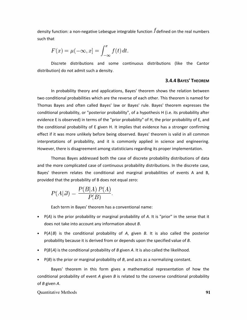
Quantitative Methods 91
density function: a non-negative Lebesgue integrable function defined on the real numbers
such that
Discrete distributions and some continuous distributions (like the Cantor
distribution) do not admit such a density.
3.4.4 BAYES' THEOREM
In probability theory and applications, Bayes' theorem shows the relation between
two conditional probabilities which are the reverse of each other. This theorem is named for
Thomas Bayes and often called Bayes' law or Bayes' rule. Bayes' theorem expresses the
conditional probability, or "posterior probability", of a hypothesis H (i.e. its probability after
evidence E is observed) in terms of the "prior probability" of H, the prior probability of E, and
the conditional probability of E given H. It implies that evidence has a stronger confirming
effect if it was more unlikely before being observed. Bayes' theorem is valid in all common
interpretations of probability, and it is commonly applied in science and engineering.
However, there is disagreement among statisticians regarding its proper implementation.
Thomas Bayes addressed both the case of discrete probability distributions of data
and the more complicated case of continuous probability distributions. In the discrete case,
Bayes' theorem relates the conditional and marginal probabilities of events A and B,
provided that the probability of B does not equal zero:
Each term in Bayes' theorem has a conventional name:
• P(A) is the prior probability or marginal probability of A. It is "prior" in the sense that it
does not take into account any information about B.
• P(A|B) is the conditional probability of A, given B. It is also called the posterior
probability because it is derived from or depends upon the specified value of B.
• P(B|A) is the conditional probability of B given A. It is also called the likelihood.
• P(B) is the prior or marginal probability of B, and acts as a normalizing constant.
Bayes' theorem in this form gives a mathematical representation of how the
conditional probability of event A given B is related to the converse conditional probability
of B given A.

92 Quantitative Methods
Bayes' theorem with continuous prior and posterior distributions
Suppose a continuous probability distribution with probability density function ƒΘ is
assigned to an uncertain quantity Θ. (In the conventional language of mathematical
probability theory Θ would be a "random variable") The probability that the event B will be
the outcome of an experiment depends on Θ; it is P(B | Θ). As a function of Θ this is the
likelihood function:
Then the posterior probability distribution of Θ, i.e. the conditional probability
distribution of Θ given the observed data B, has probability density function
Where the "constant" is a normalizing constant so chosen as to make the integral of
the function equal to 1, so that it is indeed a probability density function. This is the form of
Bayes' theorem actually considered by Thomas Bayes.
In other words, Bayes' theorem says:
To get the posterior probability distribution, multiply the prior probability
distribution by the likelihood function and then normalize.
More generally still, the new data B may be the value of an observed continuously
distributed random variable X. The probability that it has any particular value is therefore 0.
In such a case, the likelihood function is the value of a probability density function of X given
Θ, rather than a probability of B given Θ:
Bayes' Theorem derived via conditional probabilities.
To derive Bayes' theorem, start from the definition of conditional probability. The
probability of the event A given the event B is
Equivalently, the probability of the event B given the event A is
Rearranging and combining these two equations, we find

Quantitative Methods 93
This lemma is sometimes called the product rule for probabilities. Discarding the
middle term and dividing both sides by P(B), provided that neither P(B) nor P(A) is 0, we
obtain Bayes' theorem:
Of course, this lemma is symmetric in A and B, since A and B are arbitrarily-chosen
symbols, and dividing by P(A), provided that it is non-zero, gives a statement of Bayes'
theorem, in which the two symbols have changed places.
Theoretical probability distribution is classified into the following:
• Binomial Distribution
• Poisson Distribution
• Normal Distribution
• Exponential Distribution
Study Notes
Assessment
1. Differentiate between Discrete Probability distribution and continous probability
distribution
2. Explain Bayes Theorem

94 Quantitative Methods
Discussion
Discuss and solve: The table shows the probability distribution for the random variable x,
where x represents the number of CDs a person rents from a video store during a single
visit.
X p(x)
0 0.06
1 0.58
2 0.22
3 0.10
4 0.03
5 0.01
Determine whether the following is a valid probability distribution for the random variable
x.
[Hint: Since ΣP(x) = 0.97 is not equal to 1.
x = (0) (.06) + (1) (.58) + (2) (.220 + (4) (.03) + (5) (0.01)
= 1.49 CDs]
3.5 Binomial Distribution
In Probability Theory and statistics, the binomial distribution is the discrete
probability distribution of the number of successes in a sequence of n independent yes/no
experiments, each of which yields success with probability p. Such a success/failure
experiment is also called a Bernoulli experiment or Bernoulli trial. In fact, when n = 1, the
binomial distribution is a Bernoulli distribution. The binomial distribution is the basis for the
popular binomial test of statistical significance.
It is frequently used to model the number of successes in a sample of size n from a
population of size N. Since the samples are not independent (this is sampling without
replacement), the resulting distribution is a hyper geometric distribution and not a binomial
one. However, for N much larger than n, the binomial distribution is a good approximation
and is also widely used.

Quantitative Methods 95
3.5.1 PROPERTIES OF BINOMIAL DISTRIBUTION
• The experiment has n repeated trials.
• Each trial can have two possible outcomes. One is success and the other is failure.
• Here the trials are independent.
• Mean = n * P.
• Variance = n * P * (1 – P).
• Standard Deviation = sqrt[ n * P * ( 1 – P ) ].
3.5.2 BINOMIAL DISTRIBUTION FORMULA
b(x; n, P) = nCx * Px * (1 - P)n – x
Here the Notation are,
B(x; n, P) = binomial probability
X = successes
N = number of trials
P = probability of success
nCx = number of combinations of n trials, x is success.
3.5.3 EXAMPLES
An elementary example is this: roll a standard die ten times and count the number of
fours. The distribution of this random number is a binomial distribution with n = 10 and
p = 1/6.
For another example, flip a coin three times and count the number of heads. The
distribution of this random number is a binomial distribution with n = 3 and p = 1/2.
Binomial distribution is a statistical experiment which means the number of
successes in n repeated trials of a binomial experiment. It is also called Bernoulli distribution
or Bernoulli trial.
For example,
For a clinical trial, a patient may live or die. Here the researcher faces the number of
survivors and not how much time the patient lives after treatment.
We take a coin and flip it twice. Here we calculate the count of number of
heads(successes). Thus, the binomial distribution is

96 Quantitative Methods
Number of heads Probability
No head 0.25
One head 0.5
Two head 0.25
Example Problem(the Binomial Distribution)
A die is tossed 6 times. What is the probability of rolling fours on two occasions?
Solution
Here n = 6, x = 2, probability of success on a single trial = 1/ 6 or 01.167.
Therefore, The binomial probability is,
b( 2; 6, 0.167 ) = 6C2 * ( 0.167 )2 * ( 1 – 0.167)6 – 2
= ( 6! / 2! * (6-2)!) * 0.0279 * ( 0.833)4
= (6! / 2! * 4!) * 0.0279 * 0.481
= 15 * 0.0279 * 0.481
b( 2; 6, 0.167 ) = 0.201. Answer.
3.5.4 CUMULATIVE BINOMIAL PROBABILITY
It refers to the binomial probability which falls within a specified range that is
greater than or equal to a mentioned lower limit and less than or equal to a mentioned
upper limit.
For example,
Cumulative binomial probability of obtaining 5 or fewer heads in 10 tosses of a coin.
b( x <= 5; 10, 0.5)= b( x = 0; 10, 0.5) + b( x = 1; 10, 0.5) +…… + b ( x = 5; 10, 0.5)
Definition:
The binomial distribution is one of the distinct probability distributions. It is used
when there are exactly two equally exclusive outcomes of a trial. These outcomes are
appropriately labelled success and failure. The binomial distribution is used to find the
probability of observing ‘r’ successes in ‘n’ trials, with the probability of success on a single
trial denoted by ‘p’.
Formula:
P(X = r) = nCr p r (1-p) n-r

Quantitative Methods 97
where,
n = Number of events.
r = Number of successful events.
p = Probability of success on a single trial.
nCr =
1-p = Probability of failure
Example of Binomial Distribution
1.Toss a coin for 12 times. What is the probability of getting exactly 6 heads?
Solution:
Step 1: Here,
Number of trials n = 12
Number of success r = 6 (since we define getting a head as success)
Probability of success on any single trial p = 0.5
Step 2: To calculate nCr formula is used.
nCr =
=
=
=
=
= 924
Step 3: Find pr.
pr = 0.5
6
= 0.015625
Step 4: To Find (1-p)n-r Calculate 1-p and n-r.
1-p = 1-0.5 = 0.5
n-r = 12-6 = 6
Step 5: Find (1-p)n-r.
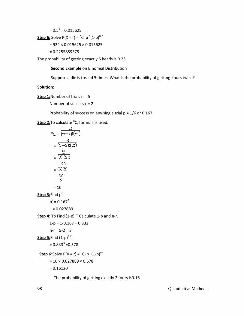
98 Quantitative Methods
= 0.56 = 0.015625
Step 6: Solve P(X = r) = nCr p r (1-p)n-r
= 924 × 0.015625 × 0.015625
= 0.2255859375
The probability of getting exactly 6 heads is 0.23
Second Example on Binomial Distribution
Suppose a die is tossed 5 times. What is the probability of getting fours twice?
Solution:
Step 1:Number of trials n = 5
Number of success r = 2
Probability of success on any single trial p = 1/6 or 0.167
Step 2:To calculate nCr formula is used.
nCr =
=
=
=
=
= 10
Step 3:Find pr.
pr = 0.1672
= 0.027889
Step 4: To Find (1-p)n-r Calculate 1-p and n-r.
1-p = 1-0.167 = 0.833
n-r = 5-2 = 3
Step 5:Find (1-p)n-r
.
= 0.8333 =0.578
Step 6:Solve P(X = r) = nCr p r (1-p)n-r
= 10 × 0.027889 × 0.578
= 0.16120
The probability of getting exactly 2 fours is0.16

Quantitative Methods 99
Study Notes
Assessment
1. What did you understand by Binomial Distribution?
2. Explain Cumulative Binomial Distribution.
Discussion
Discuss and solve: A die is tossed 6 times. What is the Probability of getting exactly 2 fours?
[ Hint:Here n = 6, x = 2, probability of success on a single trial = 1/ 6 = 0.167.
Then p = 0.167,
p + q =1
p = 1-q
Formula P(b) = ncr pr q(n-r) or q =(1-p).
Ans. b( 2; 6, 0.167 ) = 0.201]
3.6 Poisson Distribution
In Probability Theory and statistics, the Poisson distribution is a discrete probability
distribution that expresses the probability of a number of events occurring in a fixed period
of time if these events occur with a known average rate and independently of the time since
the last event. (The Poisson distribution can also be used for the number of events in other

100 Quantitative Methods
specified intervals such as distance, area or volume.)
The distribution was first introduced by Siméon-Denis Poisson (1781–1840) and
published, together with his probability theory, in 1838 in his work Recherches sur la
probabilité des jugements en matière criminelle et en matière civile (Research on the
Probability of Judgments in Criminal and Civil Matters). The work focused on certain random
variables N that count, among other things, the number of discrete occurrences (sometimes
called “arrivals”) that take place during a time-interval of given length.
If the expected number of occurrences in this interval is λ, then the probability that
there are exactly k occurrences (k being a non-negative integer, k = 0, 1, 2, ...) is equal to
where
• e is the base of the natural logarithm (e = 2.71828...)
• k is the number of occurrences of an event - the probability of which is given by the
function
• k! is the factorial of k
• λ is a positive real number, equal to the expected number of occurrences that occur
during the given interval. For instance, if the events occur on average 4 times per minute
and you are interested in probability for k times of events occurring in a 10 minute
interval, you would use a Poisson distribution with λ = 10×4 = 40 as your model.
As a function of k, this is the probability mass function. The Poisson distribution can
be derived as a limiting case of the binomial distribution.
• The Poisson distribution can be applied to systems with a large number of possible
events, each of which is rare. A classic example is the nuclear decay of atoms.
3.6.1 PROPERTIES OF POISSON DISTRIBUTION
• The expected value of a Poisson-distributed random variable is equal to λ. It is the same
for its variance. The higher moments of the Poisson distribution are Touchard
polynomials in λ, whose coefficients have a combinatorial meaning. In fact, when the
expected value of the Poisson distribution is 1, then Dobinski's formula says that the nth
moment equals the number of partitions of a set of size n.

Quantitative Methods 101
• The mode of a Poisson-distributed random variable with non-integer λ is equal to ,
which is the largest integer less than or equal to λ. This is also written as floor(λ). When λ
is a positive integer, the modes are λ and λ − 1.
• Sums of Poisson-distributed random variables:
If follow a Poisson distribution with parameter and Xi are
independent, then
also follows a Poisson distribution, whose parameter is the sum of the component
parameters. A converse is Raikov's Theorem, which says that if the sum of two independent
random variables is Poisson-distributed, then so is each of those two independent random
variables.
• The sum of normalised square deviations is approximately distributed as chi-square if
the mean is of a moderate size (λ > 5 is suggested).
If are observations from independent Poisson distributions with means
then
• The moment-generating function of the Poisson distribution with expected value λ is
• All of the cumulants of the Poisson distribution are equal to the expected value λ. The
nth factorial moment of the Poisson distribution is λn.
• The Poisson distributions are infinitely divisible probability distributions.
• The directed Kullback-Leibler divergence between Pois(λ) and Pois(λ0) is given by
3.6.2 FORMULA OF POISSON DISTRIBUTION
Formula for Poisson distribution is
• e is function of log e=2.718

102 Quantitative Methods
• is the change of rate
• is the actual success value.
3.6.3 EXAMPLE PROBLEMS
Problem1:
Solve the Poisson distribution where =8 and = 12
Step1: Given =8
= 12
e= 2.718
Step2: Formula is
Step3:
=( 2.718) -8
= 0.000335
Step4:
=(8)12
= 68719476736
Step5: Apply the values
=
=
=
= 0.048
Solution: The Poisson distribution is 0.048
Problem2:
Solve the Poisson distribution where =9 and = 11
Step1: Given =9
= 11

Quantitative Methods 103
e= 2.718
Step2: Formula is
Step3:
=( 2.718) -9
= 0.0001234
Step4:
=(9)11
= 31381059609
Step5: Apply the values
=
=
=
= 0.097
Solution: The Poisson distribution is 0.097
Problem3:
Solve the Poisson distribution where =6 and = 12
Step1: Given =6
= 12
e= 2.718
Step2: Formula is
Step3:
=( 2.718) -6
=0.00247875
Step4:
=(6)12

104 Quantitative Methods
= 2176782336
Step5: Apply the values
=
=
=
= 0.011
Solution: The Poisson distribution is 0.011.
Practice Problems for Poisson Distribution
Problem1:
Solve the Poisson distribution where =22 = 26
Solution:
The answer of the Poisson distribution where =22 = 26 is 0.055
Problem2:
Solve the Poisson distribution where =20 = 29
Solution:
The answer of the Poisson distribution where =20 = 29 is 0.013
Problem3:
Solve the Poisson distribution where =18 = 21
Solution:
The answer of the Poisson distribution where =18 = 21 is 0.068.
Problem4:
Solve the Poisson distribution where =20 = 30
Solution:
The answer of the Poisson distribution where =20 = 30 is 0.008

Quantitative Methods 105
Study Notes
Assessment
1. The number of pizza orders received at a pizza place follows a Poisson model with a
mean rate of 7 per hour.
a. What is the probability that the pizza shop goes more than 1/2hour between orders?
b. If it has been 1 hour since the last order, what is the probability that an order arrives
in less than 15 minutes?
2. A pizza shop makes deliveries, and the time to make the delivery follows a uniform
distribution between 20 and 35 (minutes): f(x) = 1/15 for 20 < x < 35.
a. Find the average delivery time and the standard deviation of the delivery times.
b. According to Chebyshev's theorem, at least 75% of the delivery times must be
between what two values?
c. On each trip, the supervisor of the drivers gives a bonus of $0.10 for each minute
below 35. For example, if a driver takes 28 minutes, that is a $0.70 bonus. What is
the average bonus per trip?
Discussion
Discuss how Poisson Distribution is different from Probability and Binomial Distribution?

106 Quantitative Methods
3.7 Normal Distribution
The distribution characterised by the continuous property is termed as normal
distribution. After a vast study, it has been concluded that data collected from the various
fields of science viz., Meteorology, Agriculture, Bioscience, Physics etc, fits the characters of
normal distribution.
Based on the consistency property of the variables of the data series, attempts have
made to evolve the mathematical models highlighting such patterns of distribution to
facilitate the investigation. According to the Statistical Theory, there are three fundamental
distributions viz., Normal, Binomial and the Poisson. The normal distribution is important
amongst them.
The normal distribution, also called the Gaussian distribution, is an important family
of continuous probability distributions, applicable in many fields as mentioned above. Every
constituent member of the family may be defined by two parametres viz., scale and
location.
If we calculate a certain statistic, i.e. parametres are the constants characterising the
population, from X1, X2, X3, ………………………. Xn, then it is found that the mean of above
series is normally distributed and when n tends mass value, the distribution of all the
statistics tends towards the normal.
The importance of the normal distribution as a model of quantitative phenomena lies
in its usage in the natural, social and behavioural sciences. Many measurements, ranging
from psychological to physical phenomena, can be approximated, to varying degrees, by
adopting the normal distribution. While the mechanisms underlying these phenomena are
often unknown, the use of the normal model can be theoretically justified by assuming that
many small, independent effects are additively contributing to each observation. The normal
distribution is also important for its relationship to least-squares estimation. It is believed to
be one of the simplest and oldest methods of statistical estimation.
The normal distribution was first introduced by Abraham de Moivre in 1733, while
the method of least squares was introduced by Legendre in 1805.
The standard normal distribution is the normal distribution with the value of a mean
equal to nil or zero and a variance of one (continuous lined curve in the graph). The
researcher, Carl F. Gauss associated this set of distributions when he analysed astronomical
data and defined the equation of its probability density function. Universally, it is termed as
the bell curve because of its graphical shape, which resembles that of a bell shape.

Quantitative Methods 107
Fig. 3.2: Normal probability density distribution
3.7.1 DEFINITION OF NORMAL DISTRIBUTION
The simplest case of a normal distribution is known as the standard normal
distribution. It is described by the probability density function
The constant in this expression ensures that the total area under the curve
ϕ(x) is equal to one and 1⁄2 in the exponent makes the “width” of the curve (measured as
half of the distance between the inflection points of the curve) also equal to one. It is
traditional in statistics to denote this function with the Greek letter ϕ (phi), whereas density
functions for all other distributions are usually denoted with letters ƒ or p. The alternative
glyph φ is also used quite often, however, within this article we reserve “φ” to denote
characteristic functions.
More generally, a normal distribution results from exponentiating a quadratic
function (just as an exponential distribution results from exponentiating a linear function):
This yields the classic “bell curve” shape (provided that a < 0 so that the quadratic
function is concave). Notice that f(x) > 0 everywhere. One can adjust a to control the
“width” of the bell, then adjust b to move the central peak of the bell along the x-axis and
finally adjust c to control the “height” of the bell. For f(x) to be a true probability density
function over R, one must choose c such that (which is only possible
when a < 0).
Rather than using a, b and c, it is far more common to describe a normal distribution

108 Quantitative Methods
by its mean μ = −b/(2a) and variance σ2 = −1/(2a). Changing to these new parametres allows
us to rewrite the probability density function in a convenient standard form,
Notice that for a standard normal distribution, μ = 0 and σ2 = 1. The last part of the
equation above shows that any other normal distribution can be regarded as a version of the
standard normal distribution that has been stretched horizontally by a factor σ and then
translated rightward by a distance μ. Thus, μ specifies the position of the bell curve’s central
peak and σ specifies the “width” of the bell curve.
The parameter μ is at the same time the mean, the median and the mode of the
normal distribution. The parametre σ2 is called the variance; as for any random variable, it
describes how concentrated the distribution is around its mean. The square root of σ2 is
called the standard deviation and is the width of the density function.
The normal distribution is usually denoted by N(μ, σ2). Commonly the letter N is
written in calligraphic font (typed as \mathcal{N} in LaTeX). Thus, when a random variable X
is distributed normally with mean μ and variance σ2, we write
3.7.2 EQUATION OF NORMAL DISTRIBUTION
In the normal distribution pattern, the area under a frequency curve represents the
total number of observations.
Let us assume this area under frequency curve is unity. Then the equation for the
normal curve will be as follows:
Where;
µ and σ are the parameters of the normal distribution
µ = mean of the population under study
σ = standard deviation of the population under study
The above mentioned equation of the normal distribution defines the Y of any value
of X located in between ± ∞ .
1 X - µµµµ
2
- -- ------
1 2 σσσσ Y = ------- e σσσσ √√√√2ππππ
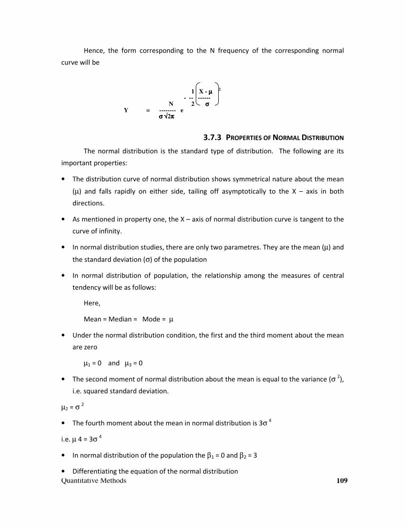
Quantitative Methods 109
Hence, the form corresponding to the N frequency of the corresponding normal
curve will be
3.7.3 PROPERTIES OF NORMAL DISTRIBUTION
The normal distribution is the standard type of distribution. The following are its
important properties:
• The distribution curve of normal distribution shows symmetrical nature about the mean
(µ) and falls rapidly on either side, tailing off asymptotically to the X – axis in both
directions.
• As mentioned in property one, the X – axis of normal distribution curve is tangent to the
curve of infinity.
• In normal distribution studies, there are only two parametres. They are the mean (µ) and
the standard deviation (σ) of the population
• In normal distribution of population, the relationship among the measures of central
tendency will be as follows:
Here,
Mean = Median = Mode = µ
• Under the normal distribution condition, the first and the third moment about the mean
are zero
µ1 = 0 and µ3 = 0
• The second moment of normal distribution about the mean is equal to the variance (σ 2),
i.e. squared standard deviation.
µ2 = σ 2
• The fourth moment about the mean in normal distribution is 3σ 4
i.e. µ 4 = 3σ 4
• In normal distribution of the population the β1 = 0 and β2 = 3
• Differentiating the equation of the normal distribution
1 X - µµµµ
2
- -- ------
N 2 σσσσ Y = -------- e σσσσ √√√√2ππππ

110 Quantitative Methods
By differentiating the equation of the normal curve twice with respect to X and
representing the derivatives by ‘Y’
we gets
1
Y’ = − ----- (X -µ) Y
σ2
and
1 X - µ 2
Y” = − ----- 1 − --------- Y
σ2 σ
• The range estimates are as follows:
� The range of µ ± σ includes about 68 % of the observations
� The range of µ ± 2σ includes about 95 % of the observations
� The range of µ ± 3σ includes about 99% of the observations
• The normal distribution shows the property that the sum and differences of normally
distributed variables are also distributed normally.
3.7.4 NORMAL VARIABLE AND NORMAL CURVE
A random variable X, whose distribution has the shape of a normal curve is called a
normal random variable.
1 X - µµµµ
2
- -- ------
1 2 σσσσ Y = ------- e σσσσ √√√√2ππππ

Quantitative Methods 111
Fig. 3.3: Normal curve
Normal Curve
This random variable X is said to be normally distributed with mean μ and standard
deviation σ if its probability distribution is given by
3.7.5 THE STANDARD NORMAL DISTRIBUTION
To simplify matters, let us standardise our normal curve, with a mean of zero and a
standard deviation of 1 unit.
If we have the standardised situation of μ = 0 and σ = 1, then we have:
Fig. 3.4: Standard normal curve
Standard Normal Curve μ = 0, σ = 1
We can transform all the observations of any normal random variable X with mean μ

112 Quantitative Methods
and variance σ to a new set of observations of another normal random variable Z with mean
0 and variance 1 by using the following transformation:
We can see this in the following example:
Example
Say μ = 2 and σ = 1/3 in a normal distribution.
The graph of the normal distribution is as follows:
Fig. 3.5: Normal distribution
μ = 2, σ = 1/3
The following graph represents the same information but it has been standardised so
that μ = 0 and σ = 1:
μ = 0, σ = 1
Fig. 3.6: Normal distribution
The two graphs have different μ and σ but have the same shape (if we alter the
axes).
The new distribution of the normal random variable Z with mean 0 and variance 1 (or

Quantitative Methods 113
standard deviation 1) is called a standard normal distribution. Standardising the distribution
like this makes it much easier to calculate probabilities.
If we have mean μ and standard deviation σ, then
Since all the values of X falling between x1 and x2 have corresponding Z values
between z1 and z2, it means:
The area under the X curve between X = x1 and X = x2 equals:
The area under the Z curve between Z = z1 and Z = z2.
Hence, we have the following equivalent probabilities:
P(x1<X<x2) = P(z1<Z<z2)
Example
Considering our example above, where μ = 2, σ = 1/3, then
One-half standard deviation = σ/2 = 1/6 and
Two standard deviations = 2σ = 2/3
So s.d. to 2 s.d. to the right of μ = 2 will be represented by the area from
to . This area is graphed as follows:
Fig. 3.7: Normal distribution
μ = 2, σ = 1/3
The area above is exactly the same as the area z1 = 0.5 to z2 = 2in the standard
normal curve:

114 Quantitative Methods
μ = 0, σ = 1
Fig. 3.8: Normal distribution
Percentages of the Area under the Standard Normal Curve
A graph of this standardised (mean 0 and variance 1) normal curve is shown.
Fig. 3.9: Normal distribution
In this graph, we have indicated the areas between the regions as follows:
-1 ≤ Z ≤ 168.27%
-2 ≤ Z ≤ 2 95.45%
-3 ≤ Z ≤ 3 99.73%
This means that 68.27% of the scores lie within 1 standard deviation of the mean.
This comes from:

Quantitative Methods 115
Also, 95.45% of the scores lie within 2 standard deviations of the mean.
This comes from:
Finally, 99.73% of the scores lie within 3 standard deviations of the mean.
This comes from:
The total area from -∞ <z< ∞ is 1.
3.7.6 THE Z-TABLE
The areas under the curve bounded by the ordinates z = 0 and any positive value of z
are found in the z-Table. From this table, the area under the standard normal curve between
any two ordinates can be found by using the symmetry of the curve about z = 0.
EXAMPLE 1
Find the area under the standard normal curve for the following, using the z-table. Sketch
each one.
a. betweenz = 0 and z = 0.78
b. betweenz = -0.56 and z = 0
c. betweenz = -0.43 and z = 0.78
d. betweenz = 0.44 and z = 1.50
e. to the right of z = -1.33.
EXAMPLE 2
Find the following probabilities:
a. P(Z> 1.06)
b. P(Z< -2.15)
c. P(1.06 <Z< 4.00)
d. P(-1.06 <Z< 4.00)
EXAMPLE 3
It was found that the mean length of 100 parts produced by a lathe was 20.05 mm,
with a standard deviation of 0.02 mm. Find the probability that a part selected at random

116 Quantitative Methods
would have a length:
a. Between 20.03 mm and 20.08 mm
b. Between 20.06 mm and 20.07 mm
c. Less than 20.01 mm
d. Greater than 20.09 mm.
EXAMPLE 4
A company pays its employees an average wage of $3.25 an hour with a standard
deviation of 60 cents. If the wages are normally distributed approximately, determine:
a. The proportion of the workers getting wages between $2.75 and $3.69 an hour
b. The minimum wage of the highest 5%
Study Notes
Assessment
1. What are the Properties of Normal Distribution?
2. Explain Normal Variable and Normal Curve.
3. What is z-Table?
Discussion
The average life of a certain type of motor is 10 years, with a standard deviation of 2 years.
If the manufacturer is willing to replace only 3% of the motors that fail, how long a
guarantee should he offer? Assume that the lives of the motors follow a normal
distribution.

Quantitative Methods 117
3.8 Exponential Distribution
In Probability Theory and statistics, the exponential distributions (a.k.a.
negative exponential distributions) are a class of continuous probability
distributions. They describe the times between events in a Poisson process, i.e. a
process in which events occur continuously and independently at a constant
average rate.
Fig. 3.10: Exponential Probability density function
Fig. 3.11: Cumulative distribution function

118 Quantitative Methods
• Probability density function
The probability density function (pdf) of an exponential distribution is
Here λ > 0 is the parameter of the distribution and is often called the rate parameter.
The distribution is supported on the interval [0, ∞). If a random variable X has this
distribution, we write X ~ Exp(λ).
• Cumulative distribution function
The cumulative distribution function is given by
• Alternative parameterisation
A commonly used alternative parameterisation is to define the probability density
function (pdf) of an exponential distribution as
where β > 0 is a scale parameter of the distribution and is the reciprocal of the rate
parameter, λ, defined above. In this specification, β is a survival parameter in the sense that
if a random variable X is the duration of time that a given biological or mechanical system
manages to survive and X ~ Exponential(β) then E[X] = β. That is to say, the expected
duration of survival of the system is β units of time. The parameterisation involving the
"rate" parameter arises in the context of events arriving at a rate λ, when the time between
events (which might be modelled using an exponential distribution) has a mean of β = λ−1
.
The alternative specification is sometimes more convenient than the one given
above and some authors will use it as a standard definition. This alternative specification is
not used here. Unfortunately, this gives rise to a notational ambiguity. In general, the reader
must check which of these two specifications is being used if an author writes
"X ~ Exponential(λ)", since either the notation in the previous (using λ) or the notation in this
section (here, using β to avoid confusion) could be intended.

Quantitative Methods 119
3.8.1 PROPERTIES OF EXPONENTIAL DISTRIBUTION
1. Mean, variance and median
The mean or expected value of an exponentially distributed random variable X with
rate parameter λ is given by
In light of the examples given above, this makes sense: if you receive phone calls at
an average rate of 2 per hour, then you can expect to wait half an hour for every call.
The variance of X is given by
The median of X is given by
where ln refers to the natural logarithm. Thus, the absolute difference between the
mean and median is
in accordance with the median-mean inequality.
2. Memorylessness
An important property of the exponential distribution is that it is memoryless. This
means that if a random variable T is exponentially distributed, its conditional probability
obeys
This says that the conditional probability that we need to wait, for example, more
than another 10 seconds before the first arrival, given that the first arrival has not yet
happened after 30 seconds, is equal to the initial probability that we need to wait more than
10 seconds for the first arrival. Thus, if we waited for 30 seconds and the first arrival did not
happen (T > 30), the probability that we will need to wait another 10 seconds for the first
arrival (T > 30 + 10) is the same as the initial probability that we need to wait more than 10
seconds for the first arrival (T > 10). This is often misunderstood by students taking courses
on probability: the fact that Pr(T > 40 | T > 30) = Pr(T > 10) does not mean that the events

120 Quantitative Methods
T > 40 and T > 30 are independent.
To summarise: "memorylessness" of the probability distribution of the waiting time T
until the first arrival means
It does not mean
(That would be independence. These two events are not independent.)
The exponential distributions and the geometric distributions are the only
memoryless probability distributions.
The exponential distribution is consequently also necessarily the only continuous
probability distribution that has a constant failure rate.
3. Quartiles
The quartile function (inverse cumulative distribution function) for Exponential(λ) is
for 0 ≤ p < 1. The quartiles are therefore:
first quartile
median
third quartile
4. Kullback–Leibler divergence
The directed Kullback–Leibler divergence between Exp(λ0) ('true' distribution) and
Exp(λ) ('approximating' distribution) is given by
5. Maximum entropy distribution
Among all continuous probability distributions with support [0,∞) and mean μ, the

Quantitative Methods 121
exponential distribution with λ = 1/μ has the largest entropy.
6. Distribution of the minimum of exponential random variables
Let X1, ..., Xn be independent exponentially distributed random variables with rate
parameters λ1, ..., λn. Then
is also exponentially distributed, with parameter
This can be seen by considering the complementary cumulative distribution function:
The index of the variable which achieves the minimum is distributed according to the
law
Note that
is not exponentially distributed.
3.8.2 OCCURRENCE AND APPLICATIONS
The exponential distribution occurs naturally when describing the lengths of the
inter-arrival times in a homogeneous Poisson process.
The exponential distribution may be viewed as a continuous counterpart of the
geometric distribution, which describes the number of Bernoulli trials necessary for a
discrete process to change state. In contrast, the exponential distribution describes the time
for a continuous process to change state.
In real-world scenarios, the assumption of a constant rate (or probability per unit
time) is rarely satisfied. For example, the rate of incoming phone calls differs according to
the time of day. On the other hand, if we focus on a time interval during which the rate is
roughly constant, such as from 2 to 4 p.m. during work days, the exponential distribution
can be used as a good approximate model for the time until the next phone call arrives.

122 Quantitative Methods
Similar caveats apply to the following examples, which yield approximately exponentially
distributed variables:
• The time until a radioactive particle decays or the time between clicks of a Geiger
counter
• The time it takes before your next telephone call
• The time until default (on payment to company debt holders) in reduced form credit risk
modelling
Exponential variables can also be used to model situations where certain events
occur with a constant probability per unit length, such as the distance between mutations
on a DNA strand or between roadkills on a given road.
In Queuing Theory, the service times of agents in a system (e.g. how long it takes for
a bank teller etc. to serve a customer) are often modelled as exponentially distributed
variables. (The inter-arrival of customers, for instance, in a system is typically modelled by
the Poisson distribution in most management science textbooks.) The length of a process
that can be thought of as a sequence of several independent tasks is better modelled by a
variable following the Erlang distribution (which is the distribution of the sum of several
independent exponentially distributed variables).
Reliability Theory and reliability engineering also make extensive use of the
exponential distribution. As a result of the memoryless property of this distribution, it is
well-suited to model the constant hazard rate portion of the bathtub curve used in reliability
theory. It is also very convenient because it is easy to add failure rates in a reliability model.
The exponential distribution is however, not appropriate to model the overall lifetime of
organisms or technical devices because the "failure rates" here are not constant: more
failures occur for very young and for very old systems.
In physics, if you observe a gas at a fixed temperature and pressure in a uniform
gravitational field, the heights of the various molecules also follow an approximate
exponential distribution.

Quantitative Methods 123
Study Notes
Assessment
1. What do you mean by Exponential Distribution?
2. What are the properties of Exponential Distribution?
Discussion
Discuss occurrence and application of Exponential Distribution.
3.9 Summary
Frequency Distribution: In statistics, a frequency distribution is a tabulation of the
values that one or more variables take in a sample. Each entry in the table contains the
frequency or count of the occurrences of values within a particular group or interval. In this
way, the table summarises the distribution of values in the sample.
Probability Theory: Probability theory is the branch of mathematics concerned with
analysis of random phenomena. Simply put, probability is the ratio of the number of
favourable cases to that of total number of equally likely or possible cases.
Probability Distribution: Probability distribution identifies either the probability of
each value of a random variable (when the variable is discrete) or the probability of the
value falling within a particular interval (when the variable is continuous).

124 Quantitative Methods
Bayes' Theorem: In probability theory and applications, Bayes' theorem shows the
relation between two conditional probabilities, which are the reverse of each other. This
theorem is named for Thomas Bayes and often called Bayes' law or Bayes' rule. Bayes'
theorem expresses the conditional probability, or "posterior probability", of a hypothesis H
(i.e. its probability after evidence E is observed) in terms of the "prior probability" of H, the
prior probability of E, and the conditional probability of E given H.
Binomial Distribution: The binomial distribution is the discrete probability
distribution of the number of successes in a sequence of n independent yes/no experiments,
each of which yields success with probability p.
Poisson Distribution: The Poisson distribution is a discrete probability distribution
that expresses the probability of a number of events occurring in a fixed period of time if
these events occur with a known average rate and independently of the time since the last
event.
Normal Distribution: The distribution characterised by the continuous property is
termed as normal distribution. The normal distribution, also called the Gaussian distribution,
is an important family of continuous probability distributions, applicable in many fields.
Exponential Distribution: The exponential distributions are a class of continuous
probability distributions. They describe the times between events in a Poisson process, i.e. a
process in which events occur continuously and independently at a constant average rate.
3.10 Self Assessment Test
Exercises
1. A random sample of 15 people is taken from a population in which 40% favour a
particular political stand. What is the probability that exactly 6 individuals in the sample
favour this political stand?
a. 0.4000
b. 0.5000
c. 0.2066
d. 0.0041
2. A normal distribution has a mean of 20 and a standard deviation of 4. Find the Z scores
for the following numbers: (a) 28 (b) 18 (c) 10 (d) 23
3. If scores are normally distributed with a mean of 35 and a standard deviation of 10, what
percent of the scores is: (a) greater than 34? (b) smaller than 42? (c) between 28 and 34?

Quantitative Methods 125
4. According to Financial Executive (July/August 1993) disability causes 48% of all mortgage
foreclosures. Given that 20 mortgage foreclosures are audited by a large lending
institution, what is the probability that less than 8 foreclosures are due to a disability?
5. Ninety percent of the trees planted by a landscaping firm survive. What is the probability
that of the next 13 trees planted:
a. at most ten will survive?
b. at least ten will survive?
c. exactly ten will survive?
Short Notes
a. Properties of Poisson distribution
b. Probability theory
c. Constructing frequency distribution table
d. Normal distribution
e. Applications of probability distributions
f. Bayes' Theorem
3.11 Further Reading
1. Basic Statistics for Management, Kazmier, L. J. and Pohl N. F., Prentice Hall Inc., 1995
2. Business Statistics by Examples, Terry, Sineich, Collier MacMillian Publishers, 1990
3. Business Statistics, Gupta, S P and Gupta M P, New Delhi, Sultan Chand, 1997
4. Linear Programming and Decision Making, Narang, A.S., 1995
5. Statistics for Behaviour and Social Scientists, Chadha, N. K., Reliance Publishing House,
1996
6. Statistics for Management, Levin Richard I. and Rubin David S, Prentice Hall Inc, 1995

126 Quantitative Methods
Assignment
• A doctor has decided to prescribe two new drugs to 200 heart patients as follows : 50 get
drug A, 50 get drug B and 100 get both the drugs A and B. The 200 patients were chosen
so that each had an 80% chance of having a heart attack if given neither drug. Drug A
reduces the probability of having of a heart attack by 35 %, drug B reduces the
probability by 20% and the two drugs when taken together work independently. If a
randomly selected patient in the programme has a heart attack, what is the probability
that he is given both the drugs? (0.4177)
• Suppose that weights of bags of potato chips coming from a factory follow a normal
distribution with mean 12.8 ounces and standard deviation .6 ounces. If the
manufacturer wants to keep the mean at 12.8 ounces but adjust the standard deviation
so that only 1% of the bags weigh less than 12 ounces, how much does he/she need to
make that standard deviation?
___________________________________________________________________________
___________________________________________________________________________
___________________________________________________________________________
___________________________________________________________________________
___________________________________________________________________________
___________________________________________________________________________
___________________________________________________________________________
___________________________________________________________________________
___________________________________________________________________________
___________________________________________________________________________
___________________________________________________________________________
___________________________________________________________________________
___________________________________________________________________________
___________________________________________________________________________
___________________________________________________________________________

Quantitative Methods 127
Unit 4 Correlation, Regression and Time Series
Learning Outcome
After reading this unit, you will be able to:
• Explain correlation
• Learn the concepts and calculation of correlation
• Identify probable error and standard error in correlation
• Study regression analysis
• Locate standard error in regression
• Elucidate on the pitfalls in regression and regression application
• Define time series
• Characterise Analysis and Models Of Time Series
Time Required to Complete the unit
1. 1st Reading: It will need 3 Hrs for reading a unit
2. 2nd Reading with understanding: It will need 4 Hrs for reading and understanding a
unit
3. Self Assessment: It will need 3 Hrs for reading and understanding a unit
4. Assignment: It will need 2 Hrs for completing an assignment
5. Revision and Further Reading: It is a continuous process
Content Map
4.1 Introduction
4.2 Correlation
4.2.1 Correlation Analysis

128 Quantitative Methods
4.2.2 Definition of Correlation
4.2.3 Concept of Correlation
4.2.4 Assumptions of Correlation Analysis
4.2.5 Measurement of Correlation
4.2.6 Coefficient of Concurrent Deviation
4.2.7 Probable Error in Correlation (P.E.)
4.2.8 Standard Error
4.2.9 Coefficient of Determination
4.3 Regression Analysis
4.3.1 Properties of Regression Coefficient
4.3.2 Standard Error Estimate
4.3.3 Pitfalls associated with Regressions
4.3.4 Real World Applications using IT tools
4.4 Time Series
4.4.1 Analysis
4.4.2 Models
4.4.3 Notations
4.4.4 Conditions
4.4.5 What is Moving Average or Smoothing Techniques?
4.5 Summary
4.6 Self Assessment Test
4.7 Further Reading

Quantitative Methods 129
4.1 Introduction
Correlation and dependence are any of a broad class of statistical relationships
between two or more random variables or observed data values.
Familiar examples of dependent phenomena include: the correlation between the
physical statures of parents and their offspring and the correlation between the demand for
a product and its price. Correlations are useful because they can indicate a predictive
relationship that can be exploited in practice. For example, an electrical utility may produce
less power on a mild day based on the correlation between electricity demand and weather.
Correlations can also suggest possible causal or mechanistic relationships; however,
statistical dependence is not sufficient to demonstrate the presence of such a relationship.
Formally, dependence refers to any situation in which random variables do not
satisfy a mathematical condition of probabilistic independence. In general statistical usage,
although correlation or co-relation can refer to any departure of two or more random
variables from independence, it most commonly refers to a more specialised type of
relationship between mean values. There are several correlation coefficients, often denoted
ρ or r, measuring the degree of correlation. The most common of these is the Pearson
correlation coefficient, which is mainly sensitive to a linear relationship between two
variables. Other correlation coefficients have been developed to be more robust than the
Pearson correlation or more sensitive to nonlinear relationships.
Regression analysis refers to the techniques used for modelling and analysis of
numerical data consisting of values of a dependent variable (response variable) and of one
or more independent variables (explanatory variables). The dependent variable in the
regression equation is modelled as a function of the independent variables, corresponding
parametres ("constants") and an error term. The error term is treated as a random variable.
It represents unexplained variation in the dependent variable. The parametres are estimated
in order to give a "best fit" of the data. Most commonly, the best fit is evaluated by using the
least squares method, although other criteria have also been used.
Regression can be used for prediction (including forecasting of time-series data),
inference, hypothesis testing and modelling of causal relationships. These uses of regression
rely heavily on the underlying assumptions being satisfied. Regression analysis has been
criticised as being misused for these purposes in many cases, where the appropriate
assumptions cannot be verified to hold. One factor contributing to the misuse of regression
is that it can take considerably more skill to criticise a model than to fit a model.
In statistics, signal processing, econometrics and mathematical finance, a time series

130 Quantitative Methods
is a sequence of data points, measured typically at successive times spaced at uniform time
intervals. Examples of time series are the daily closing value of the Dow Jones index or the
annual flow of volume of the Nile river at Aswan. Time series analysis comprises methods for
analysing time series data, in order to extract meaningful statistics and other characteristics
of the data. Time series forecasting is the use of a model to forecast future events based on
known past events: to predict data points before they are measured. An example of time
series forecasting in econometrics is predicting the opening price of a stock based on its past
performance.
4.2 Correlation
Correlation is the tendency towards interrelation variation. The measure of such a
tendency is the degree to which the two variables are interrelated and is measured by a
coefficient that is called coefficient of correlation. It gives the degree of association
between the variables.
4.2.1 CORRELATION ANALYSIS
The correlation expresses rates between the groups but not between individual
items. The relationship between two variables is not functional.
Correlation analysis is a statistical procedure by which we can determine the degree
of association or relationship between two or more variables. The amount of correlation in
a data is measured as a coefficient of correlation, which is denoted by r.
4.2.2 DEFINITION OF CORRELATION
The method that is used to find a relationship between two variables (a quantified
bivariate data) is called correlation analysis.
Croxton and Cowden defined correlation as, “The relationship is of quantitative
nature. The appropriate statistical tool for discovering and measuring the relationship and
expressing it in brief formula is known as correlation".
As per A.M. Tuttle, “Correlation is an analysis of the co-variation between two or
more variables".
4.2.3 CONCEPT OF CORRELATION
The relationship between two variables such that a change in one variable results in
a positive or negative change in the other variable and also, a greater change in one variable
results in corresponding greater or smaller change in the other variable is known as
correlation.

Quantitative Methods 131
The coefficient of correlation between two variables x, y is generally defined by r and
rxy or r(x, y) or r.
There are two types of distribution:
Univariate distribution: In this case, there is only one variable. For example, the
height of students in a class.
Bivariate distribution: In this case, there are two variables such as height and weight
of the students in a class.
Frequency: - Let (xi, yj), i = 1, 2, 3…….m
j = 1,2,3….n, be a bivariate distribution.
If the pair (xi, yj) occurs fi j times than fi j is called the frequency of the pair
(x, y) then the total frequency N= ∑=
m
1i
∑=
n
1j
(fij)
Covariance: The corresponding values of the two variables x and y on the given set of
n unit of observation is given by the pair
(x1 y1), (x2, y2), (x3,y3),……… (xn,yn)
Covariance of x, y, cov(x, y) =
[(x1 - x ) (y1- y ) + (x2 - x ) (y2- y )… (xn - x ) (yn- y )] / n
= 1/n ∑=
n
1i
(xn - x ) (yn- y )
Where x and y are mean of x1 and y1
The above formula for calculation of covariance is difficult and complicated. An
easier method of calculation is:
cov (x, y) = 1/n [∑=
n
1i
xiyj -1/n (∑=
n
1i
xi) (∑=
n
1j
yj)]
Example:
Calculate the covariance of the following pairs of observation of two variables x and y
(1, 6), (2, 9), (3, 6), (4, 7), (5, 8)
Solution:
Σ xi = 1+2+3+4+5 = 15

132 Quantitative Methods
Σ yj = 6+9+6+7+8 = 36
Σ xi yj = 6+18+18+28+40 = 110
Cov (x1y) = 1/n [∑=
n
1i
xiyj -1/n (∑=
n
1i
xi) (∑=
n
1j
yj)]
= 1
5 [110 -
1
5 (15)(36)]
= 1
5 (110 - 108) =
2
5 = 0.4
Types of Correlation
1. Positive Correlation
If the value of two variables deviates in the same direction as if an increase in one
variable (x) increases the other variable (y), then the correlation is positive or direct. The
height and weight of a growing child can be taken as an example. This is also called linear
correlation.
Fig. 4.1: Positive Correlation
2. Negative Correlation or Inverse Correlation
When two variable x and y deviate in the opposite direction, then the correlation is
said to be negative or inverse.
Fig. 4.2: Negative Correlation
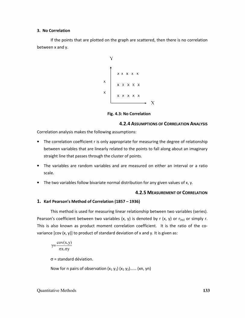
Quantitative Methods 133
3. No Correlation
If the points that are plotted on the graph are scattered, then there is no correlation
between x and y.
Fig. 4.3: No Correlation
4.2.4 ASSUMPTIONS OF CORRELATION ANALYSIS
Correlation analysis makes the following assumptions:
• The correlation coefficient r is only appropriate for measuring the degree of relationship
between variables that are linearly related to the points to fall along about an imaginary
straight line that passes through the cluster of points.
• The variables are random variables and are measured on either an interval or a ratio
scale.
• The two variables follow bivariate normal distribution for any given values of x, y.
4.2.5 MEASUREMENT OF CORRELATION
1. Karl Pearson’s Method of Correlation (1857 – 1936)
This method is used for measuring linear relationship between two variables (series).
Pearson’s coefficient between two variables (x, y) is denoted by r (x, y) or r(xy) or simply r.
This is also known as product moment correlation coefficient. It is the ratio of the co-
variance [cov (x, y)] to product of standard deviation of x and y. It is given as:
cov(x,y)γ=
σx.σy
σ = standard déviation.
Now for n pairs of observation (x1 y1) (x2 y2)…… (xn, yn)
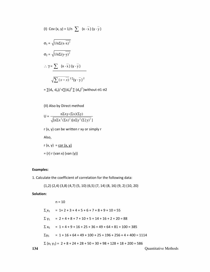
134 Quantitative Methods
(I) Cov (x, y) = 1/n ∑ (x - x ) (y - y )
σ1 = 21/nΣ(x-x)
σ2 = 21/nΣ(y-y)
∴ γ = ∑ (x - x ) (y - y )
∑ − )( xx2 ∑
(y - y ) 2
= ∑(dx. dy)/ √∑(dx)2 ∑ (dy)
2 )without σ1 σ2
(II) Also by Direct method
U = 2 2 2 2
nΣxy-(Σx)(Σy)
[nΣx (Σx) )[nΣy (Σ{y) ]
r (x, y) can be written r xy or simply r
Also,
r (x, y) = cor (x, y)
= (r) r (van x) (van (y))
Examples:
1. Calculate the coefficient of correlation for the following data:
(1,2) (2,4) (3,8) (4,7) (5, 10) (6,5) (7, 14) (8, 16) (9, 2) (10, 20)
Solution:
n = 10
Σ x1 = 1+ 2 + 3 + 4 + 5 + 6 + 7 + 8 + 9 + 10 = 55
Σ y1 = 2 + 4 + 8 + 7 + 10 + 5 + 14 + 16 + 2 + 20 = 88
Σ x5 = 1 + 4 + 9 + 16 + 25 + 36 + 49 + 64 + 81 + 100 = 385
Σy5 = 1 + 16 + 64 + 49 + 100 + 25 + 196 + 256 + 4 + 400 = 1114
Σ (x1 y1) = 2 + 8 + 24 + 28 + 50 + 30 + 98 + 128 + 18 + 200 = 586

Quantitative Methods 135
x = 55
10 = 5.5 y =
88
10 = 8
γ = n Σ x1y1 - (Σ x1) (Σ y1)
√ [[n Σ x12 - (Σ x1)2)] [n Σ y1
2 - (Σ{y1)2] ]
= 10 X 586 - 55 X 88
√10 X 385 - 55 X 55 (10 X 1114 - (88)2)
=1020
825 3396X =
1020
2801700
= 1020
1673.5 = 0.61 (approx)
2. Given below are the monthly incomes and savings of 10 employees of a company.
Calculate the correlation coefficient.
Employee 1 2 3 4 5 6 7 8 9 10
Monthly
Income
780 360 980 250 750 820 900 620 650 390
Net saving 84 51 91 60 66 62 86 58 53 47
Solution:
ξ = 6500
65010
= ; γ = 660
6610
=
No. x y x = x- ξ y = y - γ x5 y5 x y
1 780 84 130 18 16900 324 2340
2 360 51 -290 -15 84100 225 4350
3 980 91 330 25 108900 625 8250
4 250 60 -400 -6 160000 36 2400
5 750 68 100 2 10000 4 200
6 820 62 170 -4 28900 16 -680
7 900 86 250 20 62500 400 500

136 Quantitative Methods
8 620 58 -30 -8 900 64 240
9 650 53 0 -13 0 169 0
10 390 47 -260 -19 67600 361 4610
Total 6500 660 0 0 539800 2224 27040
r = 1/n (x - x ) (y - y ) / √1/n ∑ (x - x )2 1/n ∑(y - y )2
= ∑xy / √x2 y2 = 27040/ √537800 X 2224 = 0.78 approx.
The value γ indicates a high degree of association between the variables x and y.
From this we can derive that higher the income, higher will be the savings.
2. Spearman’s Rank Correlation
The coefficient of rank correlation is denoted by R.
This is applied to a problem where there is no quantitative data.
Then,
Coefficient of correlation is given by the
R = 1 - 2
2
6
( 1)
D
n n
Σ−
D2 = Square of the difference of corresponding ranks, n = number of paired
observations.
Example:
The ranking of 10 students in Statistics and Accountancy are as follows:
Statistics 3 5 8 4 7 10 2 1 6 9
Accountancy 6 4 9 8 1 2 3 10 5 7
Find the coefficient of rank correlation.
Solution:
Rank x Rank y D D5
3 6 -3 9
5 4 1 1

Quantitative Methods 137
8 9 -1 1
4 8 -4 16
7 1 6 36
10 2 8 64
2 3 1 1
1 10 9 81
6 5 1 1
9 7 2 4
Total 214
Now R = 2
2
1 6
( 1)
D
n n
− Σ=
− 2
1 6 214
10(10 1)
X−=
−=
2
1 6 214
10(10 1)
X−−
=1 6 214
990
X−
= 1- 1.3 = -0.3
Rank Correlation Coefficient
When the ranks are not given
1. Assign the rank highest first and the lowest last on both x and y
2. Find the rank difference (D), then D2
3. Apply formula as done earlier.
Example:
Calculate the coefficient of correlation from the following data by the method of rank
correlation.
x : 75 88 95 70 60 80 81 50
y : 120 134 150 115 110 140 142 100
x - Assign the highest first
95, 88, 81, 80, 75, 70, 60, 50.

138 Quantitative Methods
y - 150, 142, 140, 134, 120, 115, 110, 100
X Rank x y Rank y Rank
differences
D2
75 5 120 5 0 0
88 2 134 4 -2 4
95 1 150 1 0 0
70 6 115 6 0 0
60 7 110 7 0 0
80 4 140 3 1 1
81 3 142 2 1 1
50 8 100 8 0
ΣD2 = 6
Coefficient of rank correlation is given by
R = 2
2
1 6
( 1)
D
n n
− Σ
− n = 8
D2 = 4= 1 6 4
8(64 1)
X−−
= 1- 1
21 =
20
21 = 0.9
Merits of rank correlation coefficient:
The merits of rank correlation coefficient can be given as follows:
• Easy to understand and calculate.
• Useful for qualitative data such as beauty honesty etc.
• Useful when qualitative data is not given.
Limitations of rank correlation coefficient:
The limitations of rank correlation coefficient can be given as follows:

Quantitative Methods 139
• Cannot be used for grouped frequency distribution.
• Not as accurate as Karl Pearson’s coefficient of correlation.
• Cannot be used for more than 30 numbers of items as it consumes time.
• Cannot be used as a continuous series.
4.2.6 COEFFICIENT OF CONCURRENT DEVIATION
The underlying principle in the coefficient of concurrent deviation is as follows:
“If the short term fluctuations of two series are correlated, positively their deviation
would be concurrent and the curves would move in the same direction indicating positive
correlation between the series".
The coefficient of concurrent deviation is given by:
γc = + nc2 − /n
c = number of pairs of concurrent deviations
n = number of pairs of deviations, which one less than actual numbers N = n
= N -1
Example: Calculate the coefficient of correlation by concurrent deviation method.
Price : 1 4 3 5 5 8 10 10 11 15
Demand: 100 80 80 60 58 50 40 40 35 30
Solution:
Price
(X) Cx Demand
(y)
Cy Cx Cy
1 0 100 --
4 -- 80 -- +
3 -- 80 -- +
5 -- 60 -- +

140 Quantitative Methods
5 -- 58 -- +
8 -- 50 -- +
10 -- 40 -- +
10 -- 40 -- +
11 -- 35 -- +
15 -- 30 -- +
C = 9
Here n = N -1 = 10 -1 = 9
γc = nc2 −−+
/n = 102X9 −−+
/10
ΣPc = + 0.89
Merits:
The merits of coefficient of concurrent deviation can be given as follows:
• Simple to understand and compute
• It is useful for short term fluctuations
Limitations:
The limitations of coefficient of concurrent deviation can be given as follows:
• Not useful for long term range
• Does not differentiate between small and big variations
• The results are a rough indicator of the presence or absence of correlation
4.2.7 PROBABLE ERROR IN CORRELATION (P.E.)
Probable error of the coefficient of correlation (P.E.) can be given as:
= 0.6745 X2 2(1 ) 2 (1 )
3
r r
n n
− −= −
This helps in interpreting its value. This is subject to error of sampling.

Quantitative Methods 141
Properties of P.E.:
The properties of probable error in correlation can be given as:
• If r = 6 X PE then it is not significant.
• If, r ≤ 6 X PE then it is significant and correlation exists.
• Correlation of the population r ± D P.E. This P.E. is used for testing the reliability value of
r.
Conditions for use of P.E.
The conditions for the use of probable error in correlation can be given as:
• The sample taken should be unbiased and the individual items must be independent.
• The whole data is symmetrical and gives a normal frequency curve (bell shaped).
• The measure of P.E. must be calculated from the sample.
• The items in two series should not be independent of each other.
4.2.8 STANDARD ERROR
Standard error can be calculated using the following formula:
21SE=
r
n
−
r = Coefficient of Correlation
n = number of observations in pairs.
4.2.9 COEFFICIENT OF DETERMINATION
It is the square of the coefficient correlation
= r2, where r = coefficient of correlation
For example, if r = 0.2, r2 = 0.04.
Example:
If n = 25 and P.E. = 0.072 find the values of (i) r and (ii) standard error of
2(1 )r P.E.=0.6745
r
n
−×
n = 25
r =?

142 Quantitative Methods
PE = 0.072
20.6745 (1 )0.072 =
25
r× −
20.6745 (1 )0.072 =
5
r× −
2 0.07235(1-r ) =
0.6745=
0.360
0.6745=
360
674.5= 0.533
1 – r2 = 0.533
r2 = 1- 0.533 = 0.467
0.467r = = 0.6828
Standard error 21 r
SEn
−= n = 25
1-r2 = 0.533 (given above)
0.533
5= = 0.1066
Study Notes
Assessment
1. Explain concept of Correlation
2. What are the types of Correlation
3. What are the assumptions of correlation analysis
4. What is Probable Error and Standard Error.

Quantitative Methods 143
Discussion
It is assumed that achievement test scores should be correlated with student's classroom
performance. One would expect that students who consistently perform well in the
classroom (tests, quizes, etc.) would also perform well on a standardized achievement test
(0 - 100 with 100 indicating high achievement). A teacher decides to examine this
hypothesis. At the end of the academic year, she computes a correlation between the
students achievement test scores (she purposefully did not look at this data until after she
submitted students grades) and the overall g.p.a. for each student computed over the
entire year. The data for her class are provided below.
Achievement G.P.A.
98 3.6
96 2.7
94 3.1
88 4.0
91 3.2
77 3.0
86 3.8
71 2.6
59 3.0
63 2.2
84 1.7
79 3.1
75 2.6
72 2.9
86 2.4
85 3.4
71 2.8
93 3.7
90 3.2
62 1.6
1. Compute the correlation coefficient.
2. What does this statistic mean concerning the relationship between achievement
test prformance and g.p.a.?

144 Quantitative Methods
3. What percent of the variability is accounted for by the relationship between the two
variables and what does this statistic mean?
4. What would be the slope and y-intercept for a regression line based on this data?
5. If a student scored a 93 on the achievement test, what would be their predicted
G.P.A.? If they scored a 74? A 88?
[Answers:
1. r = .524127623 or .52
2. There is a moderate correlation between achievement test performance and g.p.a. As
the achievement test scores go up, the g.p.a.s tend to increase as well and vice versa.
3. r2 = .27 The percent a variability is relatively low. Only 27 percent of the achievement
test performance is related to the g.p.a (and vice versa). Seventy-three percent of the
variability is left unexplained.
4. The slope would be .028430629 and the y-intercept would be .62711903.
5. 3.27; 2.73; 3.13]
4.3 Regression Analysis
We have seen that correlation studies the relationship between two variables X and
Y. If the value of one variable is given and we want to estimate the value of the other
variable, we use the regression method; regression means to go back. In statistics, the term
“regression” is used to denote backward tendency, which means to go back to average or
normal.
Regression analysis is used for estimating or predicting these unknown values of a
variable (called as dependent variable) from the known values of the other variable (called
as independent variable). This is done through the regression line. This describes the
average relationship between the variable x and y.
Regression is simple (using two variables) or multiple and the relationship could be
linear (indicated by a straight line) or non linear.
There are two types of variables in regression analysis : (1) Dependent variable (2)
Independent variable
Dependent variable: The variable, whose value is influenced or is to be predicted is
called the dependent variable.

Quantitative Methods 145
Independent variable: The variable, which influences the value or is used for
prediction is called the independent variable. The independent variable is also known as
regression or predictor explanatory, while the dependent variable is called a regressed or
explained variable.
Regression equation of y on x
Straight line equation = y = a + b x (y on x) where a and b are constant representing
the Y intercept and the slope of the line respectively. a and b are obtained by solving the
normal equations
Σy = n a + b Σx
and
x y = aΣx + bΣx2
obtained from n given pairs of observations for y and x. We use the form
y - y = byx (x - x )
where byx is the regression. Coefficient of y on x which is given by
byx = Cov (x1 y) = γ σy
or 2 2
( )( )
( ) ( )yx
n xy x yb
n x x
Σ − Σ Σ=
Σ − Σ
Direct Method
Regression equation of x and y
It is expressed as x = a + b y
Σ x = n a + b Σ y
and
Σ x y = a Σ y + b Σ y2
A more convenient form
x - x = bxy (y - y )
Where, bxy is the regression coefficient of x on y which is given by
2 2
( , )xy
Cov x y y x dxdyb
y y dy
σσ σ
Σ= = =
Σ
where dx = x- x

146 Quantitative Methods
dy = y- y
or
2 2
( )( )
( ( )xy
n xy x yb
n y y
Σ − Σ Σ=
Σ − Σ
4.3.1 PROPERTIES OF REGRESSION COEFFICIENTS
1. Regression coefficients are not symmetric (byx ≠ bxy) unlike the correlation coefficients
[(rxy) = (ryx) = r]
2. Both regression coefficient bxy and byx have the same sign
3. r2 = bxy.byx ∴r = correlation coefficient between x and y
xy yxr b b∴ = ± ⋅ where r has the same sign ( + or -) as that of bxy and by
4.3.2 STANDARD ERROR ESTIMATE
It measures deviation (dispersion) of the central values about the regression line and
is given by
Syx = (standard error of estimate y for given x)
= unexplained error / n = )(e
yy∑ − 2/n
y is the actual
ye is estimated value for given x
Also, Syx = σy 1-r2
The standard error of estimate of x for given y as Sxy
2
eΣ(x-x )
n
Where, x is the actual value and xe is the estimated value of y.
Also, Sxy = σx 21 r−
Standard error of estimate measures the accuracy of the estimated figures. Smaller
its value, better are the estimates and hence more representative is the regression line.
Example:
1. The following data gives the experience of machine operators and their performance
ratings given by the number of goods turned out per 100 pieces.

Quantitative Methods 147
Operator 1 2 3 4 5 6 7 8
Experience (x) 16 12 18 4 3 10 5 12
Ratings (y) 87 88 89 68 78 80 75 83
Calculate the regression line of performance ratings on experience and estimate the
probable performance if an operator has 7 years of experience.
n = 8
We have x =x
n
Σ=
80
8 = 10
y = y
n
Σ=
81
8=81
Let us create a table.
X Y dx=x-10 dy(y-81) dx2 dy
2 dx. dy x
2 y
2 Xy
16 87 6 6 36 36 36 256 7569 1392
12 88 2 7 4 49 14 144 7744 1056
18 89 8 8 64 64 64 324 792 1602
4 68 -6 -13 36 169 78 16 4624 272
3 78 -7 -3 49 9 21 9 6884 234
10 80 0 -1 0 36 0 100 6400 800
5 75 -5 -6 25 36 30 25 5625 375
12 83 2 2 4 4 4 144 6889 996
80 648 0 0 218 318 247 1018 53676 6727
∴ byx = Σ dxdy = 247 = 1.133
Σdx2 218
By direct method:

148 Quantitative Methods
byx = 2 2 2
nΣxy-Σx)(Σy) 8X6727-80X648 1976= = =1.133
nΣx -(Σx ) 8X10¹⁸-(80) 1744
Equation of regression lines on x is
y - y = byx (x- x )
y - 81 = 1.133 (x - 10)
y - 81 = 1.133x - 11.33
y = 1.133 x + 81 - 11.33
= 1.133x + 69.67 Ans.
If experience is 7 years, the probable performance will be,
x = 7
y = 1.133 x + 69.67 = 1.133x 7 + 69.67 = 7.991 + 69.67 = 77.66 Ans.
2. From the following data
Mean X=36 Y=85
Standard deviation 11 8
Correlation coefficient between x and y is 0.66. Find the regression equation x and y
hence estimate the value of x when y = 75.
Solution:
Given x = 36, y = 85,
σx = 11 σy = 8
r = 0.66
bxy = γ x
y
σσ
= 0.66 X 11
8= 0.908
The regression equation 3on y
x - x = bxy (y- y )
x - 36 = 0.908 (y-85)
x- 36 = 0.908 y - 77.180
x = 0.908 y - 77.180 + 36 = 0.908 y - 41.180

Quantitative Methods 149
When Y = 75, then x will be
X = 0.90 8 x 75 - 41.180 = 26.92
4.3.3 PITFALLS ASSOCIATED WITH REGRESSION
Also, to the extent that there is a non-linear relationship between the two variables
to be correlated, correlation will not understand the relationship.
Correlation can also be misleading average. The relationship varies depending on the
value of the independent variable. (Lack of homoscedacity)
Homoscedacity: This means that variance around the regression line is the same for
all values of the predictor variable x. The plot shows a violation of this assumption. For the
lower values, the points are all very close to the regression line. For higher values on the x-
axis, there is much more variability around the regression line.
Fig. 4.4: Variance around the regression line
4.3.4 REAL WORLD APPLICATION USING IT TOOLS
Use of statistical methods has undergone a dramatic change as computers and
powerful calculators have emerged in everyday business environments. Companies can
store and manipulate collections of data so that once formidable statistical calculations are
now reduced to a few keystrokes. Sophisticated Windows software allows users to merely
specify the type of analysis required and input the necessary data. Some of the IT
(Information Technology) tools are:
• Microsoft Excel: Excel is a spreadsheet program that can be used to access, process,
analyse, display and share information for running a business. Excel continues to make
the existing functionality easier to use while simultaneously offering a wide array of
tools for making more advanced tasks less complex and more intuitive. Excel is not

150 Quantitative Methods
designed to be a statistical package; however, it does offer a number of built-in
statistical functions and analysis procedures.
• Minitab: Minitab is a widely used Statistical Analysis Package, originally developed in
1972 at Penn State University to help professors teach basic statistics. Over the years,
Minitab has grown into a powerful and accurate, yet easy-to-use, set of statistical tools.
Minitab is used by a number of Fortune 500 companies and by more than 4000 colleges
and universities worldwide.
• SPSS: SPSS is a large-scale statistical software package designed to integrate and
analyze marketing, customer and operational data. The letter SPSS originally meant
“Statistical Package for the Social Scientists”. Today, SPSS provides solutions that
discover what customers want and predict what they will do.
USES OF STATISTICS IN BUSINESS
Modern businesses need many future predictions in comparison to the small
businesses of the past. Small business managers used to solve most of their problems
through personal contacts. Managers in large corporations, however, must try to
summarise and analyse the various data available to them. They do this by modern
statistical methods.
Here are a list of six areas of business that rely on information and techniques:
• Quality improvement: Statistical quality-control procedures can help give assurance of
high product quality and enhance productivity.
• Product planning: Statistical methods are used to analyse economic factors and business
trends and to prepare detailed sales budgets, inventory-control systems and realistic
sales quotas.
• Forecasting: Statistics are used to predict sales, productivity and employment trends.
• Yearly reports: Annual reports for stockholders are based on statistical treatment of
many cost and revenue factors analysed by the business comptroller.
• Personnel management: Statistical procedures are used in areas of age and sex
discrimination lawsuits, performance appraisals and workforce-size planning.
• Market research: Corporations that develop and market products or services use
sophisticated statistical procedures to describe and analyse consumer purchasing
behaviour.
Quantitative Methods 151
Study Notes
Assessment
1. What are the properties of Regression Coefficients?
2. What are the drawbacks of Regression?
Discussion
Discuss real world application of regression.
4.4 Time Series
Time series data have a natural temporal ordering. This makes time series analysis
distinct from other common data analysis problems, in which there is no natural ordering of
the observations (e.g. explaining people's wages by reference to their education level, where
the individuals' data could be entered in any order). Time series analysis is also distinct from
spatial data analysis, where the observations generally relate to geographical locations (e.g.
accounting for house prices by the location as well as the intrinsic characteristics of the
houses). A time series model will generally reflect the fact that observations close together
in time will be more closely related than observations further apart. In addition, time series
models will often make use of the natural one-way ordering of time so that values for a
given period will be expressed as deriving in some way from past values, rather than from

152 Quantitative Methods
future values. (Time series: random data plus trend, with best-fit line and different
smoothing).
Methods for time series analyses may be divided into two classes: frequency-domain
methods and time-domain methods. The former include spectral analysis and recently
wavelet analysis, while the latter include auto-correlation and cross-correlation analysis.
Fig. 4.5: Time series
Definition of time series: Time series is an ordered sequence of values of a variable
at equally spaced time intervals. Time series occur frequently when looking at industrial data
Applications: The usage of time series models is twofold:
• Obtain an understanding of the underlying forces and structure that produced the
observed data
• Fit a model and proceed to forecasting, monitoring or even feedback and feedforward
control
Time series analysis is used for many applications such as:
• Economic forecasting
• Sales forecasting
• Budgetary analysis
• Stock market analysis
• Yield projections
• Process and quality control
• Inventory studies
• Workload projections
• Utility studies

Quantitative Methods 153
• Census analysis
4.4.1 ANALYSIS
There are several types of data analysis available for time series. These are
appropriate for the following different purposes:
General exploration
• Graphical examination of data series
• Autocorrelation analysis to examine serial dependence
• Spectral analysis to examine cyclic behaviour which need not be related to seasonality.
For example, sunspot activity varies over 11 year cycles. Other common examples
include celestial phenomena, weather patterns, neural activity, commodity prices and
economic activity.
Description
• Separation into components representing trend, seasonality, slow and fast variation,
cyclical irregular: see decomposition of time series
• Simple properties of marginal distributions
Prediction and forecasting
• Fully-formed statistical models for stochastic simulation purposes in order to generate
alternative versions of the time series, representing what might happen over non-
specific time-periods in the future.
• Simple or fully-formed statistical models to describe the likely outcome of the time series
in the immediate future, given knowledge of the most recent outcomes (forecasting).
4.4.2 MODELS
Models for time series data can have many forms and represent different stochastic
processes. When modelling variations in the level of a process, three broad classes of
practical importance are the autoregressive (AR) models, the integrated (I) models and the
moving average (MA) models. These three classes depend linearly on previous data points.
Combinations of these ideas produce Autoregressive Moving Average (ARMA) and
Autoregressive Integrated Moving Average (ARIMA) models. The Autoregressive Fractionally
Integrated Moving Average (ARFIMA) model generalises the former three. Extensions of
these classes to deal with vector-valued data are available under the heading of multivariate
time-series models and sometimes the preceding acronyms are extended by including an

154 Quantitative Methods
initial "V" for "vector". An additional set of extensions of these models is available for use,
where the observed time-series is driven by some "forcing" time-series (which may not have
a causal effect on the observed series): the distinction from the multivariate case is that the
forcing series may be deterministic or under the experimenter's control. For these models,
the acronyms are extended with a final "X" for "exogenous".
Non-linear dependence of the level of a series on previous data points is of interest,
partly because of the possibility of producing a chaotic time series. However, more
importantly, empirical investigations can indicate the advantage of using predictions derived
from non-linear models over those from linear models.
Among other types of non-linear time series models, there are models to represent
the changes of variance along time (heteroskedasticity). These models are called
Autoregressive Conditional Heteroskedasticity (ARCH). Here, changes in variability are
related to or predicted by, recent past values of the observed series. This is in contrast to
other possible representations of locally-varying variability, where the variability might be
modelled as being driven by a separate time-varying process, as in a doubly stochastic
model.
In recent work on model-free analyses, wavelet transform based methods (for
example, locally stationary wavelets and wavelet decomposed neural networks) have gained
favour. Multiscale (often referred to as multiresolution) techniques decompose a given time
series, attempting to illustrate time dependence at multiple scales.
The general representation of an autoregressive model, known as AR(p), is
where the term εt is the source of randomness and is called white noise. It is
assumed to have the following characteristics:
1.
2.
3.
With these assumptions, the process is specified up to second-order moments and
subject to conditions on the coefficients, may be second-order stationary.
If the noise also has a normal distribution, it is called normal white noise (denoted
here by Normal-WN):
Quantitative Methods 155
In this case, the AR process may be strictly stationary, again subject to conditions on
the coefficients.
Many types of data are collected over time. Stock prices, sales volumes, interest
rates and quality measurements are typical examples. Owing to the sequential nature of the
data, special statistical techniques that account for the dynamic nature of the data are
required.
The following procedures are followed for analysing time series data:
• Descriptive Methods: Time sequence plots, autocorrelation functions, partial
autocorrelation functions, periodograms and cross-correlation functions are all
important tools for characterizing time series data.
• Smoothing: A variety of smoothers are available to estimate the underlying trend in a
time series.
• Seasonal Decomposition: Decomposes time series data into trend, cycle, seasonal and
irregular components and returns seasonally adjusted data if desired.
• Forecasting: Creation of forecasts beyond the end of the data, using trend models,
moving averages, exponential smoothers or ARIMA models.
• Automatic Forecasting: Selects the best forecasting method for a time series by
optimising a specified information criterion.
DESCRIPTIVE METHODS
Characterising a time series involves estimating not only a mean and standard
deviation but also the correlations between observations separated in time. Tools such as
the autocorrelation function are important for displaying the manner in which the past
continues to affect the future. Other tools, such as the periodogram, are useful when the
data contain oscillations at specific frequencies.

156 Quantitative Methods
Fig. 4.6: Descriptive Methods
SMOOTHING
When a time series contains a large amount of noise, it can be difficult to visualise
any underlying trend. Various linear and nonlinear smoothers are provided to separate the
signal from the noise.
Fig. 4.7: Smoothing
SEASONAL DECOMPOSITION
When the data contain a strong seasonal effect, it is often important to separate the
seasonality from the other components in the time series. This enables one to estimate the
seasonal patterns and to generate seasonally adjusted data.
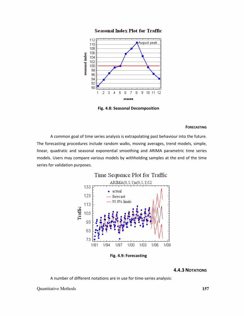
Quantitative Methods 157
Fig. 4.8: Seasonal Decomposition
FORECASTING
A common goal of time series analysis is extrapolating past behaviour into the future.
The forecasting procedures include random walks, moving averages, trend models, simple,
linear, quadratic and seasonal exponential smoothing and ARIMA parametric time series
models. Users may compare various models by withholding samples at the end of the time
series for validation purposes.
Fig. 4.9: Forecasting
4.4.3 NOTATIONS
A number of different notations are in use for time-series analysis:

158 Quantitative Methods
X = {X1, X2, ...}
is a common notation, which specifies a time series X, which is indexed by the natural
numbers. Another common notation is:
Y = {Yt: t∈T}.
4.4.4 CONDITIONS
There are two sets of conditions under which much of the theory is built:
• Stationary process
• Ergodicity
However, ideas of stationarity must be expanded to consider two important ideas:
strict stationarity and second-order stationarity. Both models and applications can be
developed under each of these conditions, although the models in the latter case might be
considered as only partly specified.
In addition, time series analysis can be applied, where the series are seasonally
stationary or non-stationary. Situations where the amplitudes of frequency components
change with time can be dealt with in time-frequency analysis, which makes use of a time–
frequency representation of a time-series or signal.
4.4.5 WHAT IS MOVING AVERAGE OR SMOOTHING TECHNIQUES?
Smoothing data removes random variation and shows trends and cyclic components.
Inherent in the collection of data taken over time is some form of random variation. There
exist methods for reducing or cancelling the effect due to random variation. An often-used
technique in industry is "smoothing". This technique, when properly applied, reveals more
clearly the underlying trend, seasonal and cyclic components.
There are two distinct groups of smoothing methods
• Averaging Methods
• Exponential Smoothing Methods
Taking averages is the simplest way to smooth data. We will first investigate some
averaging methods, such as the "simple" average of all past data.
A manager of a warehouse wants to know how much a typical supplier delivers in
1000 dollar units. He/she takes a sample of 12 suppliers, at random, obtaining the following
results:

Quantitative Methods 159
Supplier Amount Supplier Amount
1 9 7 11
2 8 8 7
3 9 9 13
4 12 10 9
5 9 11 11
6 12 12 10
The computed mean or average of the data = 10. The manager decides to use this as
the estimate for expenditure of a typical supplier.
Is this a good or bad estimate?
Mean squared error is a way to judge how good a model is. We shall compute the
"mean squared error":
• The "error" = true amount spent minus the estimated amount.
• The "error squared" is the error above, squared.
• The "SSE" is the sum of the squared errors.
• The "MSE" is the mean of the squared errors.
MSE results for example The results are:
Error and Squared Errors
The estimate = 10
Supplier $ Error Error Squared
1 9 -1 1
2 8 -2 4
3 9 -1 1

160 Quantitative Methods
4 12 2 4
5 9 -1 1
6 12 2 4
7 11 1 1
8 7 -3 9
9 13 3 9
10 9 -1 1
11 11 1 1
12 10 0 0
The SSE = 36 and the MSE = 36/12 = 3. Table of MSE results for example using
different estimates. So how good was the estimator for the amount spent for each supplier?
Let us compare the estimate (10) with the following estimates: 7, 9 and 12. That is, we
estimate that each supplier will spend $7 or $9 or $12.
Performing the same calculations we arrive at:
Estimator 7 9 10 12
SSE 144 48 36 84
MSE 12 4 3 7
The estimator with the smallest MSE is the best. It can be shown mathematically that
the estimator that minimises the MSE for a set of random data is the mean.
The above table shows squared error for the mean for sample data.
Next, we will examine the mean to see how well it predicts net income over time.
The next table gives the income before taxes of a PC manufacturer between 1985
and 1994.
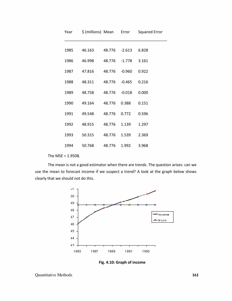
Quantitative Methods 161
Year $ (millions) Mean Error Squared Error
1985 46.163 48.776 -2.613 6.828
1986 46.998 48.776 -1.778 3.161
1987 47.816 48.776 -0.960 0.922
1988 48.311 48.776 -0.465 0.216
1989 48.758 48.776 -0.018 0.000
1990 49.164 48.776 0.388 0.151
1991 49.548 48.776 0.772 0.596
1992 48.915 48.776 1.139 1.297
1993 50.315 48.776 1.539 2.369
1994 50.768 48.776 1.992 3.968
The MSE = 1.9508.
The mean is not a good estimator when there are trends. The question arises: can we
use the mean to forecast income if we suspect a trend? A look at the graph below shows
clearly that we should not do this.
Fig. 4.10: Graph of income

162 Quantitative Methods
Average weighs all past observations equally. In summary, we state that
• The "simple" average or mean of all past observations is only a useful estimate for
forecasting when there are no trends. If there are trends, use different estimates that
take the trend into account.
• The average "weighs" all past observations equally. For example, the average of the
values 3, 4, 5 is 4. We know, of course, that an average is computed by adding all the
values and dividing the sum by the number of values. Another way of computing the
average is by adding each value divided by the number of values or
3/3 + 4/3 + 5/3 = 1 + 1.3333 + 1.6667 = 4.
The multiplier 1/3 is called the weight. In general:
The are the weights and of course they sum to 1.
Study Notes
Assessment
What is Time Series? Explain the procedures followed for analsing time series data.
Discussion
What is Smoothing?
What is Forecasting?
Discuss.

Quantitative Methods 163
4.5 Summary
Definition of Correlation: Croxton and Cowden definition of correlation: “The
relationship is of quantitative nature. The appropriate statistical tool for discovering and
measuring the relationship and expressing it in brief formula is known as correlation".
Correlation Coefficient: Correlation is the tendency towards interrelation variation
and the coefficient of correlation is a measure of such a tendency is the degree to which the
two variables are interrelated and is measured by a coefficient that is called coefficient of
correlation. It gives the degree of association between the variables.
Karl Pearson’s method of correlation: This method is used for measuring the linear
relationship between two variables (series). Pearson’s Coefficient between two variables (x,
y) is denoted by r (x, y) or r(xy) or simply r. This is also known as product moment correlation
coefficient.
σ = standard déviation.
Spearman’s Rank correlation: The coefficient of rank correlation is denoted by R.
This is applied to a problem where there is no quantitative data.
Concurrent deviation: The principle underlying in the coefficient of concurrent
deviation is as follows: “If the short term fluctuations of two series are correlated positively,
their deviation would be concurrent and the curves would move in the same direction
indicating positive correlation between the series”.
Coefficient of determination: It is square of the Coefficient Correlation
= r2, where r = Coefficient of Correlation
Regression: Regression analysis is used for estimating or predicting these unknown
values of a variable (called as dependent variable) from the known values of other (called as
independent variable). This is done through regression line. This describes the average
relationship between the variable x and y.
Properties of Regression Coefficient:
1. Regression coefficients are not symmetric (byx ≠ bxy) unlike the correlation coefficients
[(rxy) = (ryx) = r]
2. Both regression coefficient bxy and byx have the same sign.
3. r2 = bxy.byx ∴r = correlation coefficient between x and y
xy yxr b b∴ = ± ⋅ where r has the same sign (+ or -) as that of bxy and by
164 Quantitative Methods
Time Series: A time series is a sequence of data points, measured typically at
successive times spaced at uniform time intervals. Examples of time series are the daily
closing value of the Dow Jones index or the annual flow volume of the Nile River at Aswan.
Time Series Analysis: Time series analysis comprises methods for analysing time
series data, in order to extract meaningful statistics and other characteristics of the data.
Time Series Forecasting: Time series forecasting is the use of a model to forecast
future events based on known past events: to predict data points before they are measured.
An example of time series forecasting in econometrics is predicting the opening price of a
stock based on its past performance.
Application of Time Series Analysis: Time series analysis is used for many
applications such as:
• Economic Forecasting
• Sales Forecasting
• Budgetary Analysis
• Stock Market Analysis
• Yield Projections
• Process and Quality Control
• Inventory Studies
• Workload Projections
• Utility Studies
• Census Analysis
Procedures for analysing time series data: Following are the procedures followed for
analysing time series data:
• Descriptive Methods
• Smoothing
• Seasonal Decomposition
• Forecasting
• Automatic Forecasting

Quantitative Methods 165
4.6 Self Assessment test
Exercises:
1. Calculate Karl Pearson’s Coefficient of Correlation for the data given below taking 66 and
63 are assumed means of x and y respectively.
Height of Husband x (in Inches) 60 62 64 66 68 70 72
Height of Wife y (in Inches) 61 63 63 63 64 65 62
Ans.: γ = 0.939
2. Calculate Coefficient and Correlation and problem error from the following data.
X 1 2 3 4 5 6 7 8 9 10
Y 20 16 14 10 10 9 8 7 6 5
Ans.: - r = 0.95; P.E. (r) = 0.0208
3. Obtain two lines of regression for the following data:
X 43 44 46 40 44 42 45 42 38 40 42 57
Y 29 31 19 18 19 27 27 29 41 30 26 10
Also find the value of the Correlation Coefficient between x and y. (hint):-
r = _ xy xxb Xb+
Ans.: y = -1.22x + 78.67; x = -0.44y + 54.80; r = -0.7326
4. Given Below is the information about advertising and sales.
Advt exp (in Lakhs) Sales (Rs Lakh)
Mean 10 90
S.D. 3 12
Correlation Coefficient = 0.8
a. Calculate two regressions lines
b. Find the likely sales when advertising expenditure is Rs 15 lakhs

166 Quantitative Methods
c. What should be the advertising expenditure if the company sales target is of Rs. 120
lakhs
(Ans)
a. Y = 3.2 x + 58X = 0.2y - 8,
b. 106 lakh,
c. 10 lakh.
Short Notes
a. Measurement of correlation
b. Standard error
c. Correlation coefficient
d. Regression
e. Real world application using IT tools
f. Time series
4.7 Further Reading
1. Basic Statistics for Management, Kazmier, L. J. and Pohl N. F., Prentice Hall Inc., 1995
2. Business Statistics by Examples, Terry, Sineich, Collier MacMillian Publishers, 1990
3. Business Statistics, Gupta, S P and Gupta M P, New Delhi, Sultan Chand, 1997
4. Linear Programming and Decision Making, Narang, A.S., 1995
5. Statistics for Behaviour and Social Scientists, Chadha, N. K., Reliance Publishing House,
1996
6. Statistics for Management, Levin Richard I. and Rubin David S, Prentice Hall Inc, 1995

Quantitative Methods 167
Assignment
1. Calculate Karl Pearson Coefficient of Correlation from the following data:
2. From the following data obtain the two regression equation:-
X 12 4 20 8 16
Y 18 22 10 16 14
___________________________________________________________________________
___________________________________________________________________________
___________________________________________________________________________
___________________________________________________________________________
___________________________________________________________________________
___________________________________________________________________________
___________________________________________________________________________
___________________________________________________________________________
___________________________________________________________________________
___________________________________________________________________________
___________________________________________________________________________
___________________________________________________________________________
___________________________________________________________________________
___________________________________________________________________________
___________________________________________________________________________
___________________________________________________________________________
___________________________________________________________________________
___________________________________________________________________________
Year 1985 1986 1987 1988 1989 1990 1991 1992
Index of
production
100 102 104 107 105 112 103 99
Number of
unemployed
15 12 13 11 12 12 19 26

168 Quantitative Methods
___________________________________________________________________________
___________________________________________________________________________
___________________________________________________________________________
___________________________________________________________________________
___________________________________________________________________________
___________________________________________________________________________
___________________________________________________________________________
___________________________________________________________________________
___________________________________________________________________________
___________________________________________________________________________
___________________________________________________________________________
___________________________________________________________________________
___________________________________________________________________________
___________________________________________________________________________
___________________________________________________________________________
___________________________________________________________________________
___________________________________________________________________________
___________________________________________________________________________
___________________________________________________________________________
___________________________________________________________________________
___________________________________________________________________________
___________________________________________________________________________
___________________________________________________________________________
___________________________________________________________________________
___________________________________________________________________________
___________________________________________________________________________
___________________________________________________________________________
___________________________________________________________________________
___________________________________________________________________________
___________________________________________________________________________
___________________________________________________________________________

Quantitative Methods 169
Unit 5 Linear Programming
Learning Outcome
After reading this unit, you will be able to:
• Define linear programming
• Explain basic concepts and formulation of linear programming
• Apply methods of solving linear programming
• Analyse graphical method & simplex method
• Describe duality theorem
Time Required to Complete the unit
1. 1st
Reading: It will need 3 Hrs for reading a unit
2. 2nd
Reading with understanding: It will need 4 Hrs for reading and understanding a
unit
3. Self Assessment: It will need 3 Hrs for reading and understanding a unit
4. Assignment: It will need 2 Hrs for completing an assignment
5. Revision and Further Reading: It is continuous process
Content Map
5.1 Introduction
5.2 Basic Concept of Linear Programming
5.2.1 Basic Concepts
5.2.2 Limitations of Linear Programming
5.3 Formulation of Linear Programming
5.4 Solution Methods
5.4.1 Graphical method

170 Quantitative Methods
5.4.2 Simplex method
5.5 The Duality Theorem
5.6 Application of Liner Programming
5.7 Summary
5.8 Self Assessment Test
5.9 Further Reading

Quantitative Methods 171
5.1 Introduction
Linear programming (L.P.) is one of most widely and best understood Operation
Research (OR) techniques. L.P. is confined to the allocation of scarce resources among
various activities in an optimal manner. It determines the way to achieve the best outcome
(such as maximum profit or lowest cost) in a given mathematical model and given some list
of requirements represented as linear equations. Linear programming is a considerable field
of optimisation for several reasons.
This technique originated during world war in order to overcome the use of military
resources. After the war, the industries started using this technique for optimal allocation of
their resources. L.P. is always used for minimising cost and maximising profit in
manufacturing industries and various other industries. Many practical problems in
operations research can be expressed as linear programming problems.
5.2 Basic Concept of Linear Programming 5.2.1 BASIC CONCEPTS
• Linearity assumption: The term linearity means straight line or proportional relationship
with x and y. For example, if one machine and one worker produce, say 100 units per
week, then two machines and two workers will produce 200 units per work (doubled).
i.e. there is a linearity between men and machines.
• Process and its level: Conversion of an input into an output is called a conversion
process. In a process, factor of production is used in fixed ratio, depending upon
technology and as such no substitution is possible within a process. There are many
processes available to a firm for production of a product. One process can be substituted
for another. There is, thus, no interference of one with another. Two or more processes
can be used simultaneously. If a product can be produced in two different ways, then
there are two different processes/ activities/ decision variables.
• Criterion function: This is also known as objective function. This states that
determinants of the quantity are either to be maximised or minimised. For example,
revenue is profit, which needs to be maximized or cost is a function which needs to be
minimised. An objective function should include all possible activities with the revenue
(profit) or cost coefficient per unit of production. The goal is to maximise or minimise
this function. In symbolic form, Zx or Z(x) denotes the value of objective function at the X
level of activities. This is the total sum of activities produced at a specified level.
Activities are denoted as j = 1, 2 … n. The revenue or cost coefficient of the j activity is
represented by C j. Thus, Z(X), implies that for X unit of activity, j = 1 may yield a profit

172 Quantitative Methods
or loss of C j = 2.
• Inequalities (constraints): This is a restriction imposed on decision variable.
• Feasible solutions: Feasible solutions are all those possible solutions, which can be
worked upon under given constraints.
• Optimum solution: Optimum solution is the best of feasible solution.
Linear programming relationship:
L.P. deals with problems, in which the objective function as well as the constraints
can be expressed as linear mathematical functions of the decision variables.
• Direct proportional line 2X-3Y etc.
• Divisibility variable can take fractional value
e.g. p = ax + by + cz (linear function)
p = ax2 + byx + cz (quadratic function)
p = ax3 + bx2y + cx + dz (cubic function)
5.2.2. LIMITATIONS OF LINEAR PROGRAMMING
Important limitations of linear programming are as under:
• There is no guarantee that linear programming will give integer valued solutions. For
instance, a solution may result in producing a fraction / decimal. In such a situation, the
manager will examine the possibility of producing higher or lower product and will take a
decision, which ensures higher profits subject to given constraints. Thus, rounding can
give reasonably good solutions in many cases but in some situations we will get only a
poor answer even by rounding. Then integer programming techniques alone can handle
such unknown.
• Under linear programming approach, uncertainty is not allowed. The linear
programming model operates only when values for costs, constraints, etc are known but
in real life such factors may be unknown.
• The assumption of linearity is another formidable limitation of linear programming. The
objective functions and the constraint functions in the L.P. model are all linear. We are,
thus, dealing with a system that has constant returns to scale. In many situations, the
input-output rate for an activity varies with the activity level. The constraints in real life
situations concerning business and industrial problems are not linearly related to the
variables. In most economic situations, sooner or later, the law of diminishing marginal

Quantitative Methods 173
returns begins to operate. In this context, it can, however, be stated that non linear
programming techniques are available for dealing with such situations.
• Linear programming will fail to give a solution if management has multiple conflicting
goals. In L.P. model there is only one goal, which is expressed in the objective function,
e.g. maximising the value of the profit function or minimising the cost function. One
should resort to Goal Programming (G.P.) in situations involving multiple goals.
All these limitations of linear programming indicate only one thing: that linear
programming cannot be made use of in all business problems. Although linear programming
is certainly not a panacea for all management and industrial problems, for those problems
where it can be applied, linear programming is considered a very useful and powerful tool.
Study Notes
Assessment
What is Linear Programming?
Explain the concept of Linear Programming?
Discussion
Discuss the limitations of Linear Programming.

174 Quantitative Methods
5.3 Formulation of Linear Programming
Formulation means expressing a problem in a convenient mathematical form. Let us
discuss this with an example.
Example:
A carpentry firm manufactures tables and chairs. Data given below are the resources
used and unit profit in manufacturing a table and chair. In this problem there are two
resources namely wood and labour, which are required to produce table and chair. The firm
wants to determine the total profit by maximising the quantity to be produced. The problem
is as given below for formulation in the L.P.P. model.
Unit
requirements
Unit
requirements
Amount
Available
Resources Table Chair
Wood (sq ft) 35 30 350
Labour 10 20 150
Unit profit (Rs) 5 10
Formulation Let X1 - number of table to be produced
Let X2 - number of chair to be produced
Objective function:
Total profit consists of the profit derived from selling a table at. Rs. 5/ per table plus
the profit derived by selling a chair at Rs. 10/.
Hence, profit earned by selling tables = 5X1
Profit earned by selling chair = 10 X2
This needs to be maximized
Z maximize 5x1 + 10x2 -- objective function
Maximize Z, where Z = 5x1 + 10x2
Such that
35x1 + 30x2 ≤ 350
10x1 + 20x2 ≤ 150

Quantitative Methods 175
x1, x2 ≥ 0
Let us discuss constrains
1. Wood available for table and chair
35 X1 + 30 X2 ≤ 350 (available wood)
(≤ less than or equal to)
Second constraint is labour. This can be expressed in the same way.
10 X1 + 20 X2 ≤ 150 (available labour)
In this, we cannot have negative production, i.e. even when the plant is idle. X1 ≥ 0
and X2 ≥ 0. This is called non-negativity constraints.
Problem can be stated as follow,
• Max Z = 5 X1 + 10X2 objective function.
• 35X1 + 30X2 ≤ 300 constraint
• 10X1 + 20X2 ≤ 150 constraint
and
• X1 ≥ 0 and X2 ≥ 0 non negative condition.
Study Notes
Assessment
Explain how can you express Linear Programming in mathematical form. Give suitable
example.

176 Quantitative Methods
Discussion
Express in mathematical form:
A farmer needs to buy up to 25 cows for a new herd. He can buy either brown
cows (x) at $50 each or black cows (y) at $80 each and he can spend a total of
no more than $1600. He must have at least 9 of each type. On selling the cows he makes a
profit of $50 on each brown cow and $60 on each black cow.
5.4 Solution Methods
L.P. problems can be solved by two methods:
• Graphical method
• Simplex method
5.4.1 GRAPHICAL METHOD
Graphical method of solving L.P. problems involves two decision variables, x1 and x2.
It includes two major steps:
• Determination of the solution space that defines the feasible solution.
• Determination of optimal solution from feasible region
For example, a furniture manufacturing company plans to make two products hardly,
chairs and tables, from its available resources which consist of 400 cubic feet of mahogany
timber and 450 man hours of labour. It knows that to make a chair it requires 5 cubic feet of
timber and 10 man hours and yields a profit of Rs 80/-. To manufacture a table, it requires
20 cubic feet of timber and 15 man hours and yields a profit of Rs. 90/-. The problem is to
determine how many chairs and tables the company can make keeping within the resources
constraints so that is maximises the profit. Formulate L.P.P. model and provide its graphical
solution.
Graphical method for solving L.P.P.
This method has used two variables (X1 and X2)
Let X1 is denoted for chair.

Quantitative Methods 177
X2 is denoted for table.
Resources Chair Table Amount
Available
Wood 5 20 400
Labour (man hours) 10 15 450
Formulation
5 X1 + 20 X2 ≤ 400
10X1 + 15 X2 ≤ 450
Z max = 45 X1 + 80 X2 subject to
5 X1 + 20 X2 ≤ 400 i.e. X1 + 4X2 ≤ 80 - - - - (a)
10 X1 + 15 X2 ≤ 450 i.e. 2 X1 + 3 X2 ≤ 90 - - -(b)
X1 X2 ≥ 0
Converting
(a) and (b) to equality, we get
X1 + 4 X2 = 80 . . . . .(1)
2X1 + 3X2 = 90 . . . (2)
Step-1. Let us take the equation (1) i.e
X1 + 4 X2 = 80
Put X1 = 0 i.e. 4 X2 = 80 ∴ X2 = 20
Coordinate (0, 20)
Put X2 = 0, X1 = 80 coordinate (80, 0)
Step -2. Let us take the equation (2)
2 X1 + 3 X2 = 90
Put X1 = 0 3 X2 = 90 X2 = 30 coordinate (0, 30)
Put X2 = 0 2 X1 = 90 X1 = 45 coordinate (45, 0)

178 Quantitative Methods
Plot this point on the graph. Let us take table on X axis
Chair on Y axis
Fig. 5.1:L.P.P graph
Two straight lines intersect at point B. Its coordinates are calculated as follows:
X1 + 4 X2 = 80 (1)
2X1+ 3 X2 = 90 (2)
Multiply equation (1) by 2
2 X1 + 8X2 = 160
2 X1 + 3 X2 = 90
5 X2 = 70 ∴X2 = 14
∴X1 + 4 × 14 = 80
X1 = 24
i.e. point B in the graph
To find the value of the objective function
Max Z= 45 X1 + 80 X2
90
80
70
60
50
40
30
20
10
00
( 0, 20 )
( C-45,0 )
Table
( 0, 30 )
( B-14,24)
C
H
A
I
R
S

Quantitative Methods 179
Coordinate of
corner point
Objective function
45 X1 + 80 X2 = Z max Value
(0, 0) 45 X0 + 80 X0 = 0 0
(0, 20) 0 + 1600 1600
(24, 14) 45 × 24 + 80 × 14 2220
(45, 0) 45 × 45 + 80 × 0 2025
This maximum profit is obtained at B i.e. 24 chairs and 14 tables and is equal to
2220.
5.4.2 SIMPLEX METHOD
In the graphical solution, a search for optimal solution is limited to only corner point
of feasible solution region. This problem can be solved manually also, with two variables (x
and y) and less number of constraints. For bigger problems, an efficient procedure is
available for getting optimal solution. This is one of the main objectives of simplex method.
This is a systematic procedure called Algorithm. This method moves from one corner point
to another corner point, till optimal solution is obtained, always improving the objective
function. This method was developed by Prof. George B. Dantzig to solve L.P. problems
involving many variables and constraints.
Let us write down the problem, given earlier:
Zmax = 45 X1 + 80 X2
5 X1 + 20 X2 ≤ 400
10 X1 + 15 X2 ≤ 450
X1, X2 ≥ 0
The inequality constraint must be converted into equality constraint so that the
problem can be solved by adding slack variable to each constraint. Each slack variable
represents unused resources (machine capacity or man hour or materials etc).
Slack variable(s) is non negative. This is added to the “less than” type of constraint to
make it an equality. Always remember that slack variable(s) is added to the equation
(resources availability).
The problem can be stated as follows:

180 Quantitative Methods
Zmax = 45 X1 + 80 X2 + S1 + S2
subject to 5 X1 + 20 X2 + S1 = 400
10 X1 + 15 X2 + S2 = 450
and X1, X2, S1, S2 ≥ 0
The problem can be tabulated as follows:
Key Row Key Column
Cj Contribution/unit 45 80 0 0 Min. ratio
Basic variable. Solution
Variable X1 X2 S1 S2
0 S1 400 5 20 1 0 400/20=20
0 S2 450 10 15 0 1 450/15=30
Contribution Loss/Unit(Z j) 0 0 0 0 Z = 0
Net Contribution (Cj - Zj) 45 80 0 0
Explanation for the above table:
First row of the table indicates the value of Cj, the coefficient of objective function
and indicates contribution per unit to the objective function of each of the variables. The
second row of the table provides column headings for the table.
The first column heading lies of coefficient of the objective function of the current
basic variable. Second column represents the basic variables in the current solution.
The next column with the heading ‘Solution Values’ is the current solution. In the
example, when the solution is at origin the basic variables are the slack variable S1 and S2
These are listed in second column of the table. Referring back to the first column, the
coefficient for these two variables in the objective functions are S1 = 0 and S2 = 0
respectively. If the current solution at the origin is X1 = 0 and X2 = 0, then the solution values
correspond to S1 = 400 and S2 = 450 as shown in the last column of the table. The column
headed by X1, X2, S1, S2 are the efficient of the constraint set.
The Zj row represents the decrease in the value of the objective function that will

Quantitative Methods 181
result if one unit of the j the value is brought into solution. Hence, the Z j is a objective
function contribution loss per unit and is found out by adding the product, of C j column and
the coefficient in the constraint set, associated uni-responding basic variable. In the
example, contribution loss per unit (Zj) row values is determined as follows:
Contribution loss per unit (Zj) = Addition of (coefficients of Cj column multiplied by
corresponding coefficients of the constraint set.)
Ci Z j = 0 × 30 + 0 × 10 = 0
Similarly, values of Z j of the column can be calculated and shown in the above table
the last row (C j - Zj) represents net contribution per unit and is determined by subtracting
the appropriate Zj value from the corresponding coefficient C j value in the objective
function for that column. The value (C j - Z j) is the difference between the contribution C j
and the lost Zj that result from one unit of X j being produced. To find out the value of the
last row (Cj - Zj), the necessary calculations are shown as below:
Net contribution per unit is (Cj - Zj).
In the example, (Cj - Zj) for X1 column is: (45 – 0) = 45
Similarly, other columns can be calculated as is shown in the table above.
When (Cj - Zj) is positive, that means that there is an improvement possible in the
existing solution. The objective is to maximise profit, therefore consider the column where
contribution per unit is maximum. In this case, the X2 column contribution per unit is Rs.
80/- (maximum). This helps us to know the variable to be entered into the solution in the
beginning. Thus, X2 is the entering variable. The column corresponding in the entering
variable is known as ‘Key Column’.
Since it is decided to enter one variable as the basic variable into the solution basic,
hence one existing variable is to be departed from solution basic and replace entering
variable to be departed is identified by forming the ratios of solution values to physical rates
of substitution of entering variable. Thus, in the example given above, we have
For, S1= 400/20 = 20
S2 = 450/15 = 30
Hence, departing variable is one which is minimum, i.e. S1 is the departing variable in
our example. This procedure guarantees that there is no negative value in the basic
variable. The row corresponding to the departing variable is called ‘Key Row’. The
intersection of the element of Key Row and Key Column is called the Key Element and is

182 Quantitative Methods
demoted by this (box) in the simplex table.
• The Simplex Method: Minimisation Case
Until now, we have limited the application of the simplex method only to
maximisation problem. Now that you have developed some familiarity and understanding of
the simplex method, we can apply it to a minimisation problem.
Another way to minimise the problem is to convert the problem by multiplying the
objective function by 1. This yields negative solution values whose sign must be reversed for
application. However this approach is not recommended, since a direct solution is more
convenient to use.
• The Simplex Method (Mixed Constraints)
A situation may arise when the constraints are of mixed type. To simplify the
problem, we can change the last constraint of less than or equal to (≤) type into a equality
(=) type in the problem. Its modified formulation of LP problem can now be written as given
below:
Min Z = 60X1 + 80X2
Subject to X2 ≥ 200
X1 ≤ 400
X1 + X2 = 500
And X1 X2 ≥ 0.
The problem can be converted into the standard form by adding slack, surplus and
artificial variables in the set of constraints and assigning appropriate costs to these variables
in the objective function.
• Some Important Points
DEGENERACY
Sometimes, a linear programming problem may have a degenerate situation.
Degeneracy is revealed when a basic variable acquires a zero value (rather than a negative
or positive value) or in the final solution, either the number of basic variables is not equal to
the number of constraints or the number of zero variables does not equal the number of
decision variables. A tie for an existing variable and an arbitrary selection for it usually
precede the instance of degeneracy. If this is resolved by a proper selection of pivot
element, degeneracy can be avoided.

Quantitative Methods 183
NON-FEASIBLE SOLUTION
A linear programming problem may be unsolved mathematically due to the
contradictory nature of the constraints. Such an instance is referred to as a non-feasible
solution. A solution is also non-feasible if an artificial variable appears in the basis of the
solution purported to be optimal.
UNBOUNDED SOLUTION
If the coefficient of the entering variable is either negative or zero, implying that this
variable can be increased indefinitely without ever violating feasibility, the maximisation
problem has an unbounded solution.
MULTIPLE SOLUTIONS
The optimal solution may not be unique if one of the non-basic variables has a zero
coefficient in the final Zj - Cj row. This implies that bringing this zero coefficient non-basic
variable in the basis will neither increase nor decrease the value of the objective function.
Thus, the problem has an alternate solution, which is also optimal.
Study Notes
Assessment
Complete the sentence by choosing the correct answer the choices given:
linear programming problems are solved with the computer the meaning of the computer
output and linear programming concepts can be gained by analyzing a simple two-variable
problem with the ———method.
a) Linear programming
b) Graphic method
c) 2-Way method
d) All the above

184 Quantitative Methods
Discussion
Hale Company manufactures products A and B, each of which requires two processes,
grinding and polishing. The contribution margin is $3 for A and $4 for B. A graph showing
the maximum number of units of each product that can be processed in the two
departments identifies the following corner points: A = 0, B = 20; A = 20, B = 10; A = 30, B =
0. What is the combination of A and B that maximizes the total contribution margin?
[Answer: (a = 0, b = 20); $3(0) + $4(20) = $80 CM
(a = 20, b = 10); $3(20) + $4(10) = $100 CM - Maximum CM
(a = 30, b = 0); $3(30) + $4(0) = $90 CM]
5.5 The Duality Theorem
For every linear programming problem, there is another intimately related linear
programming problem referred to as its dual. The duality theorem states that for every
maximisation (or minimisation) problem in linear programming there is a unique similar
problem of minimisation (or maximisation) involving the same data, which describes the
original problem. The original problem is referred to as the ‘primal’. The ‘dual’ of a ‘dual’
problem is the ‘primal’. Further, the maximum feasible value of the primal objective
function equals the minimum feasible value of the dual objective function. This means that
the solutions of the primal and the dual problems are related, which yield several
advantages.
The transformation of a given primal problem into a dual problem involves the
following considerations:
• If the objective of the primal is maximisation, the objective of dual is minimisation.
• The primal has m-constraints, while its dual has m-unknowns.
• The primal has n-unknowns, while its dual has n-constraints.
• The n-coefficients of the objective function of primal (cj) become the n-constant terms of
its dual.
• The n-constant terms of the primal (bi) become the m-constant terms of the objective
function of its dual.

Quantitative Methods 185
• The coefficients of the variables of the primal (aij) are transformed in their position in
the dual, i.e. they become aij with respect to the position held in the primal.
• The n-variables (Xn) of the primal are replaced by the m new variables (Ym) of its dual.
This change affects the system of restrictions as well as the objective function.
• The sign of the inequalities in the set of restrictions of the primal (≤) is reversed in the
set of restrictions is its dual (/) and vice-versa. Readers should note that while writing
dual of the primal problem, all the given constraints of the primal should first be
changed in an uniform pattern, say of the z type constraints. This can easily be done as
stated below:
If the constraints is 2X1,+X2 /2, it can also be written as -2X1, -X2 ≤ -2. But if the
constraint is an equation such as
5X1 + 10 X2 ≤150, it can be stated in the form
-5X1 - 10X2 ≤ - 150 without changing the meaning of the given equation.
• The sign of the inequalities restricting the variable (≥ x j) non-negative values in the
primal is equal to the inequality sign of the new variable
(≤ - yj) of its dual.
Thus, by application of these considerations,
Maximise:
Z = 2X1 + 3X2
Subject to:
2X1 + X2 ≤20
X1 + 2X2 ≤20
and
X1, X2 ≥ 0
Transforms to its dual as follows:
Minimise:
Zy = 20Y1 + 20Y2
Subject to:
2Y1 + Y2 / 2

186 Quantitative Methods
Y1 + 2Y2/3
and
Y1, Y2 ≥ 0
It is instructive to note that the simplex method automatically identifies the dual
basic solution. The optimal value of the objective function remains the same as in the primal
problem. Given an optimal solution of the primal problem, the dual variable acquires the
coefficient of the slack variable in the optimal objective function equation as its optimal
value. In view of all this, it is possible to identify the dual solution from the primal solution.
Exercise
A carpenter makes chairs and tables. Processing of these products is done on
machine A and B. A chair requires 2 hours of machine A and B hours of machine B while a
table requires 5 hours of machine A but does not require machine B. Machine A and B are
available for 16 hours and 20 hours per day respectively. Profits gained by the carpenter per
chair and per table are Rs. 20/- and Rs. 100/- respectively. What should be the daily
production of the two products to realize maximum gain? Formulate LPP.
Hint: Maximise Z = 20 x1 + 100 x2
S.t 2x1 + 5x2 ≤16,
6x1 ≤ 20, x1, x2 ≥ 0
Where x1 = no. of chairs, x2 = No. of tables
Study Notes
Assessment
Explain Duality Theorem in your own words.
Quantitative Methods 187
Discussion
Discuss how Duality Theorem can be applied in real world.
5.6 Application of Linear Programming
Linear programming (LP) is a significant field of optimization for several reasons.
Many practical problems in operations research can be expressed as linear programming
problems. Certain special cases of linear programming, such as network flow problems and
multicommodity flow problems are considered important enough to have generated much
research on specialized algorithms for their solution. A number of algorithms for other types
of optimization problems work by solving LP problems as sub-problems. Historically, ideas
from linear programming have inspired many of the central concepts of optimization theory,
such as duality, decomposition, and the importance of convexity and its generalizations.
Likewise, linear programming is heavily used in microeconomics and company management,
such as planning, production, transportation, technology and other issues. Although the
modern management issues are ever-changing, most companies would like to maximize
profits or minimize costs with limited resources. Therefore, many issues can be
characterized as linear programming problems.
The areas where LPP is applied are as under:
1. Production and Operations Management
In the process industry, a given raw material can often be made into a wide variety of
products. In the oil industry, for example, crude oil is refined into gasoline, kerosene, home-
heating oil, and various grades of engine oil. There are various profit margins for each
product and it becomes important to determine the best product mix. There are several
limitations such as restrictions on the capacities, raw-material availability, demands and
supply, and any government restrictions on the output of certain products. In such cases,
LPP serves as a useful tool in decision making.
2. Human Resources
Human Resources planning problems can also be solved with linear programming.
For example, in telephone industry, the requirement of installer-repair people is seasonal.
The problem is to determine the number of installer-repair staff and line-repair staff to have
on payroll each month; so the total costs of hiring, layoffs, overtime, and regular-time wages

188 Quantitative Methods
are minimized. With the use of LPP models such problems can be solved.
3. Marketing
The right mix of media publicity in an advertising campaign is essential decision for
marketing team, where linear programming can prove to be useful tool. For example, the
media available are radio, television, and newspapers. The aim is to decide how many
advertisements are to be placed in each medium. Here, the cost of placing an advertisement
varies for various medium. The aim of every department in organisation is minimisation of
the total cost; here the aim of marketing department thus is minimisation of total cost of the
advertising campaign, keeping in mind the constraints.
4. Distribution
Another application of linear programming is in the area of distribution. For example,
there are a specified number of factories that must ship goods to a given number of
warehouses. One factory could make shipments to any number of warehouses. Here, the
cost of shipping one unit of product from a factory to warehouse is important variable. The
main aim is to minimize the total shipping costs. This decision is subject to various
constraints. Keeping in mind all the constraints and aim of the department, LPP is used to
take suitable decision.
The uses of linear programming are not limited to these five areas but allow you to
easily see why linear programming is so important and how it can practically be applied to
many areas of decision-making.
Study Notes
Assessment
Explain the application of Linear Programming

Quantitative Methods 189
Discussion
Discuss how Linear Programming is useful for Marketing?
5.7 Summary
Linear Programming: Linear programming has become the most orderly used
mathematical technique in solving a variety of problems related with management- from
scheduling, media selection, financial planning to capital budgeting, transportation and
many others. The special characteristic that linear programming always expects is to
maximise or minimise some quantity. One of the main advantages of linear programming is
that it fits strictly with reality. However, it has limitations too. The most important is the
achievement of goals. It fails to give a solution, where the management has multiple goals.
Basic Concepts: The basic concepts are as follows:
• Linearity assumption: The term linearity means straight line or proportional relationship
with x and y
• Process and its level: Conversion of an input into an output is called a conversion
process. In a process, factor of production are used in fixed ratio, of course, depending
upon technology and as such no substitution possible within a process.
• Criterion function: This is also known as objective function. This states that determinants
of the quantity either to be maximised or minimised.
• Inequalities (Constraints): This a restriction imposed on decision variable.
• Feasible solutions: Feasible solutions are all those possible solutions, which can be
worked upon under given constraints.
• Optimum solution: Optimum solution is the best of a feasible solution.
Linear programming relationship: L.P. deals with problems, in which the objective
function, as well as the constraints, can be expressed as linear mathematical functions of the
decision variables.
Formulation of L.P.: Formulation means expressing a problem in a convenient
mathematical form.
Methods of solving: L.P. problems can be solved by two methods: Graphical method
and Simplex method.

190 Quantitative Methods
Graphical method: Graphical method of solving L.P. problems involves two decision
variables x1 and x2. It includes two major steps:
• Determination of the solution space that defines the feasible solution.
• Determination of optimal solution from feasible region
Simplex method: This was developed by Prof. George B. Denting to solve L.P.
problems. In the graphical solution, a search for optimal solution was limited to only a
corner point of feasible solution region. This problem can be solved manually also, with two
variables (x and y) and lesser number of constraints. For a bigger problem, an efficient
procedure is available for getting optimal solution. This is one of the main objectives of
simplex method. This is a systematic procedure called algorithm. This method moves from
one corner point to another corner point, till optimal solution is obtained, always improving
the objective function.
The Duality Theorem: For every linear programming problem, there is another
intimately related linear programming problem referred to as its dual. The duality theorem
states that for every maximisation (or minimisation) problem in linear programming, there is
a unique similar problem of minimisation (or maximisation) involving the same data, which
describes the original problem. The original problem is referred to as the ‘primal’. The ‘dual’
of a ‘dual’ problem is the ‘primal’.
5.8 Self Assessment Test
Broad Questions
1. What is linear programming? List some problems that can be solved with the help of
linear programming. What characteristics must a problem have if linear programming is
to be used?
2. Describe simplex method of solving a linear programming problem. Why is the simplex
method considered superior to the graphic method?
Short Notes
a. Concepts and assumptions of L.P.
b. Limitations of linear programming
c. Multiple and unbounded solutions
d. Graphical method of solving linear programming problem
e. Duality theorem

Quantitative Methods 191
Numerical Exercises:
1. Maximise: P = 1.4X1 + X9
Subject to: X1≤ 3
2X1 + X2 ≤ 8
3X1 + 4X2 ≤24
and X1/ 0, X2 /0.
2. Maximise: Z = X1 + X2
Subject to: X1 + X2 ≤3
2X1 + 3X2 ≤18
X1 ≤ 6
and X1, X2 > 0
5.9 Further Reading
1. Basic Statistics for Management, Kazmier, L. J. and Pohl N. F., Prentice Hall Inc., 1995
2. Business Statistics by Examples, Terry, Sineich, Collier MacMillian Publishers, 1990
3. Business Statistics, Gupta, S P and Gupta M P, New Delhi, Sultan Chand, 1997
4. Linear Programming and Decision Making, Narang, A.S., 1995
5. Statistics for Behaviour and Social Scientists, Chadha, N. K., Reliance Publishing House,
1996
6. Statistics for Management, Levin Richard I. and Rubin David S, Prentice Hall Inc, 1995

192 Quantitative Methods
Assignment
Comment in your own words, how linear programming is an important part of quantitative
techniques.
___________________________________________________________________________
___________________________________________________________________________
___________________________________________________________________________
___________________________________________________________________________
___________________________________________________________________________
___________________________________________________________________________
___________________________________________________________________________
___________________________________________________________________________
___________________________________________________________________________
___________________________________________________________________________
___________________________________________________________________________
___________________________________________________________________________
___________________________________________________________________________
___________________________________________________________________________
___________________________________________________________________________
___________________________________________________________________________
___________________________________________________________________________
___________________________________________________________________________
___________________________________________________________________________
___________________________________________________________________________
___________________________________________________________________________
___________________________________________________________________________

Quantitative Methods 193
Glossary
Business mathematics: The mathematics used by commercial enterprises to record
and manage business operations. Mathematics typically used
in commerce includes elementary arithmetic, such as fractions,
decimals, and percentages, elementary algebra, statistics and
probability
Business Statistics: The science of good decision making in the face of uncertainty
and is used in many disciplines such as financial analysis,
econometrics, auditing, production and operations including
services improvement, and marketing research
Co-efficient: A numerical value (between +1 and -1) that identifies the
strength of the linear relationship between variables. A value
of +1 indicates an exact positive relationship, -1 indicates an
exact inverse relationship, and 0 indicates no predictable
relationship between the variables
Correlation coefficient: A statistical measure referring to the relationship between two
random variables. It is a positive correlation when each
variable tends to increase or decrease as the other does, and a
negative or inverse correlation if one tends to increase as the
other decreases
Function: A function f of a variable x is a rule that assigns to each number
x in the function's domain a single number f(x). The word
"single" in this definition is very important
Markov Chain: Sequence of stochastic events (based on probabilities instead
of certainties) where the current state of a variable or system
is independent of all past states, except the current (present)
state. Movements of stock/share prices, and growth or decline
in a firm's market share, are examples of Markov chains. It is
named after the inventor of Markov analysis, the Russian
mathematician Andrei Andreevich Markov (1856-1922)
Matrices: Flat (two-dimensional) table, in which the elements or entries
appear at the intersections of rows and columns, governed by
certain rules. They are called rectangular array in mathematics

194 Quantitative Methods
Mean: The average of a numerical set. It is found by dividing the sum
of a set of numbers by the number of members in the set
Median: The value of a numerical set that equally divides the number of
values that is larger and smaller
Mode: The value of a numerical set that appears with the greatest
frequency
Moving Average: moving average is a form of average which has been adjusted
to allow for seasonal or cyclical components of a time series.
Moving average smoothing is a smoothing technique used to
make the long term trends of a time series clearer
Normal Distribution: Also called "bell curve," the normal distribution is the curved
shape of a graph that is highest in the middle and lowest on
the sides
Poisson distribution: The distribution of number of events in a given time, arising
from a Poisson process. This differs from the binomial
distribution in that there is no upper limit, corresponding to
the parameter 'n' of a Binomial Process, to the number of
events which may occur
Probability: The measure of how likely it is for an event to occur. The
probability of an event is always a number between zero and
100%. The meaning (interpretation) of probability is the
subject of theories of probability. However, any rule for
assigning probabilities to events has to satisfy the axioms of
probability
Regression Analysis: A technique used for the modelling and analysis of numerical
data consisting of values of a dependent variable (response
variable) and of one or more independent variables
(explanatory variables)
Sequence: An ordered set, whose elements are usually determined based
on some function of the counting numbers
Series: The sum of the terms of a sequence. Finite sequences and
series have defined first and last terms, whereas infinite
sequences and series continue indefinitely