1

Unit 1 Mathematical Methods

Chapter 6: Polynomials

Objectives

To add, subtract and multiply polynomials.

To divide polynomials.

To use the remainder theorem, factor theorem and rational-root theorem to identify the linear factors of cubic and quartic polynomials.

To solve equations and inequalities involving cubic and quartic polynomials.

To recognise and sketch the graphs of cubic and quartic functions.

To find the rules for given cubic graphs.

To apply cubic functions to solving problems.

To use the bisection method to solve polynomial equations numerically.

6A – The language of polynomials A Polynomial function follows the rule

𝒚 = 𝒂𝒏𝒙𝒏 + 𝒂𝒏−𝟏𝒙𝒏−𝟏 + …………. 𝒂𝟏𝒙 + 𝒂𝟎 𝒏 ∈ 𝑵

Where 𝑎0, 𝑎1, … … … … 𝑎𝑛 are coefficients.

Degree of a polynomial is the highest power of 𝑥 with a non-zero coefficient. In summary:

2

Example 1

Let 𝑄(𝑥) = 2𝑥6 − 𝑥3 + 𝑎𝑥2 + 𝑏𝑥 + 20. If 𝑄(−1) = 2𝑄(2) = 0, find the values of 𝑎 and 𝑏.

■ The arithmetic of polynomials The operations of addition, subtraction and multiplication for polynomials are naturally defined. The sum, difference and product of two polynomials is a polynomial. Example 2

Let 𝑓(𝑥) = 𝑥3 − 2𝑥2 + 𝑥, 𝑔(𝑥) = 2 − 3𝑥 and ℎ(𝑥) = 𝑥2 + 𝑥, simplify the following: a) 𝑓(𝑥) + ℎ(𝑥) b) 𝑔(𝑥)ℎ(𝑥)

3

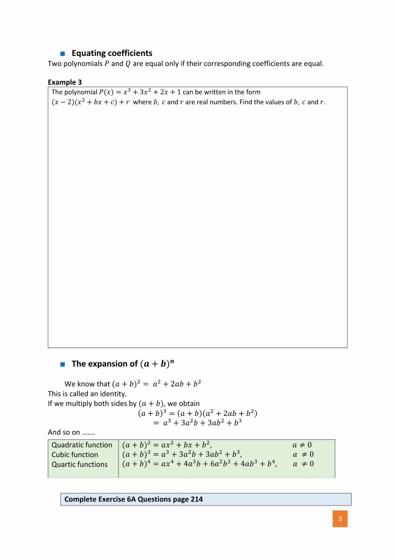
■ Equating coefficients Two polynomials 𝑃 and 𝑄 are equal only if their corresponding coefficients are equal.

Example 3 The polynomial 𝑃(𝑥) = 𝑥3 + 3𝑥2 + 2𝑥 + 1 can be written in the form

(𝑥 − 2)(𝑥2 + 𝑏𝑥 + 𝑐) + 𝑟 where 𝑏, 𝑐 and 𝑟 are real numbers. Find the values of 𝑏, 𝑐 and 𝑟.

■ The expansion of (𝒂 + 𝒃)𝒏 We know that (𝑎 + 𝑏)2 = 𝑎2 + 2𝑎𝑏 + 𝑏2 This is called an identity. If we multiply both sides by (𝑎 + 𝑏), we obtain

(𝑎 + 𝑏)3 = (𝑎 + 𝑏)(𝑎2 + 2𝑎𝑏 + 𝑏2) = 𝑎3 + 3𝑎2𝑏 + 3𝑎𝑏2 + 𝑏3

And so on …….

Complete Exercise 6A Questions page 214

Quadratic function Cubic function Quartic functions

(𝑎 + 𝑏)2 = 𝑎𝑥2 + 𝑏𝑥 + 𝑏2, 𝑎 ≠ 0 (𝑎 + 𝑏)3 = 𝑎3 + 3𝑎2𝑏 + 3𝑎𝑏2 + 𝑏3, 𝑎 ≠ 0 (𝑎 + 𝑏)4 = 𝑎𝑥4 + 4𝑎3𝑏 + 6𝑎2𝑏2 + 4𝑎𝑏3 + 𝑏4, 𝑎 ≠ 0

4

6B – Division of polynomials

In order to sketch the graphs of many cubic and quartic functions (as well as higher degree polynomials) it is often necessary to find the x-axis intercepts. As with quadratics, finding x-axis intercepts can be done by factorising and then solving the resulting equation using the null factor theorem. All cubic functions will have at least one x-axis intercept. Some will have two and others three.

Examples of long division:

1. Divide 𝑥3 − 4𝑥2 − 11𝑥 + 30 by 𝑥 − 2.

2. Divide 2𝑥3 − 6𝑥2 − 10𝑥 + 25 by 𝑥2 − 2

5

Complete Exercise 6B Questions page 219

6C – Factorisation of polynomials

■ Remainder theorem and factor theorem

Examples :

1. Find the remainder when 𝑃(𝑥) = 3𝑥4 − 9𝑥2 + 27𝑥 − 8 is divided by 𝑥 − 2.

6

2. Factorise 𝑃(𝑥) = 𝑥3 − 4𝑥2 − 11𝑥 + 30 by 𝑥 − 2 and hence solve for 𝑥.

3. Given 𝑥 + 1 and 𝑥 − 2 are factors of 6𝑥4 − 𝑥3 + 𝑎𝑥2 − 6𝑥 + 𝑏, find 𝑎 and 𝑏.

■ Sums and differences

7

Examples:

1. Factorise 27𝑥3 − 1 2. Factorise 8𝑎3 + 125𝑏3

■ The rational-root theorem

Examples:

Use the rational-root theorem to factorise 𝑃(𝑥) = 3𝑥3 + 8𝑥2 + 2𝑥 − 5.

8

■ Alternative method for division of polynomials

Synthetic division is an alternative method to long division that can be used when factorising a polynomial, and the method is not the priority.

Complete Exercise 6C Questions page 227

9

6D – Solving cubic equations

In order to solve a cubic equation, the first step is often to factorise. Apply the same rule(s) practiced in Exercise 6C to find a factor(s) or by other means, then equate to zero to find solutions. Examples:

1. Solve each of the following: a) 2(𝑥 − 1)3 = 32

b) 2𝑥3 − 𝑚𝑥2 − 22𝑥 + 11𝑚

2. Solve 2𝑥3 − 5𝑥2 + 5𝑥 − 2 = 0

Complete Exercise 6D Questions page 231

10

6E – Cubic functions of the form 𝒇(𝒙) = 𝒂(𝒙 − 𝒉)𝟑 + 𝒌 In Chapter 3 we saw that all quadratic functions can be written in ‘turning point form’ and that the graphs of all quadratics have one basic form, the parabola. This is not true of cubic functions. Consider cubic functions in the form 𝑓(𝑥) = 𝑎(𝑥 − ℎ)3 + 𝑘. The graphs of these functions can be formed by simple transformations of the graph of 𝑓(𝑥) = 𝑥3. For example, the graph of 𝑓(𝑥) = (𝑥 − 1)3 + 3 is obtained from the graph of 𝑓(𝑥) = 𝑥3 by a translation of 1 unit in the positive direction of the 𝑥-axis and 3 units in the positive direction of the 𝑦-axis.

■ Transformations of the graph 𝒇(𝒙) = 𝒙𝟑 Dilations from an axis and reflections in an axis to cubic functions in the form 𝒇(𝒙) = 𝒂𝒙𝟑

It should be noted that the implied domain of all cubics is ℝ and the range is also ℝ. The point of inflection can move as described in the above function 𝑓(𝑥) = (𝑥 − 1)3 + 3

General form:

Sketch the graph

This point is called the point of inflection (a point of

zero gradient)

𝑓(𝑥)

𝑥

Point of inflection is (1,3)

Dilation factor Horizontal translation

Vertical translation

11

■ The function 𝒇: ℝ → ℝ, 𝒇(𝒙) = 𝒙𝟏

𝟑 The functions with rules of the form 𝑓(𝑥) = 𝑎(𝑥 − ℎ)3 + 𝑘 are one-to-one functions. Hence each of these functions has an inverse function.

The inverse function of 𝑓(𝑥) = 𝑥3 is 𝑓−1(𝑥) = 𝑥1

3. Examples:

1. Sketch the graph of 𝑓(𝑥) = −2(𝑥 + 1)3 + 1. Show all intercepts andpoint of inflection.

2. Find the inverse functin of 𝑓(𝑥) = −2(𝑥 + 1)3 + 1.

𝑓(𝑥)

12

Complete Exercise 6E Questions page 235

6F – Graphs of factorised cubic functions The general cubic function written in polynomial form is

𝒚 = 𝒂𝒙𝟑 + 𝒃𝒙𝟐 + 𝒄𝒙 + 𝒅 The graph of a cubic function can have one, two or three 𝑥-axis intercepts.

■ If a cubic can be written as the product of three linear factors, 𝑦 = 𝑎(𝑥 − 𝛼)(𝑥 − 𝛽)(𝑥 − 𝛾)

then its graph can be sketched by following these steps: ▪ Find the 𝑦-axis intercept. ▪ Find the 𝑥-axis intercepts. ▪ Prepare a sign diagram. ▪ Consider the 𝑦-values as 𝑥 increases to the right of all 𝑥-axis intercepts. ▪ Consider the 𝑦-values as 𝑥 decreases to the left of all 𝑥-axis intercepts.

■ If there is a repeated factor to the power 2, the 𝑦-values have the same sign

immediately to the left and right of the corresponding 𝑥-axis intercept. Linear factors will be written as 𝑦 = 𝑎(𝑥 − 𝛼)(𝑥 − 𝛽)2

Graphs of some cubic functions

Points of

inflection

Repeated factors

Three intercepts, no repeated factors

13

■ Sign diagrams A sign diagram is a number-line diagram which shows when an expression is positive or negative. The following is a sign diagram for a cubic function, the graph of which is also shown.

Using a sign diagram requires that the factors, and the 𝑥-axis intercepts, be found. The 𝑦 −axis intercept and sign diagram can then be used to complete the graph. Example:

1. Sketch the graph of 𝑦 = (𝑥 + 1)(𝑥 − 2)(𝑥 + 3). Hint: draw a sign diagram first.

2. Sketch the graph of 𝑦 = 3𝑥3 − 4𝑥2 − 13𝑥 − 6

14

Complete Exercise 6F Questions page 241

15

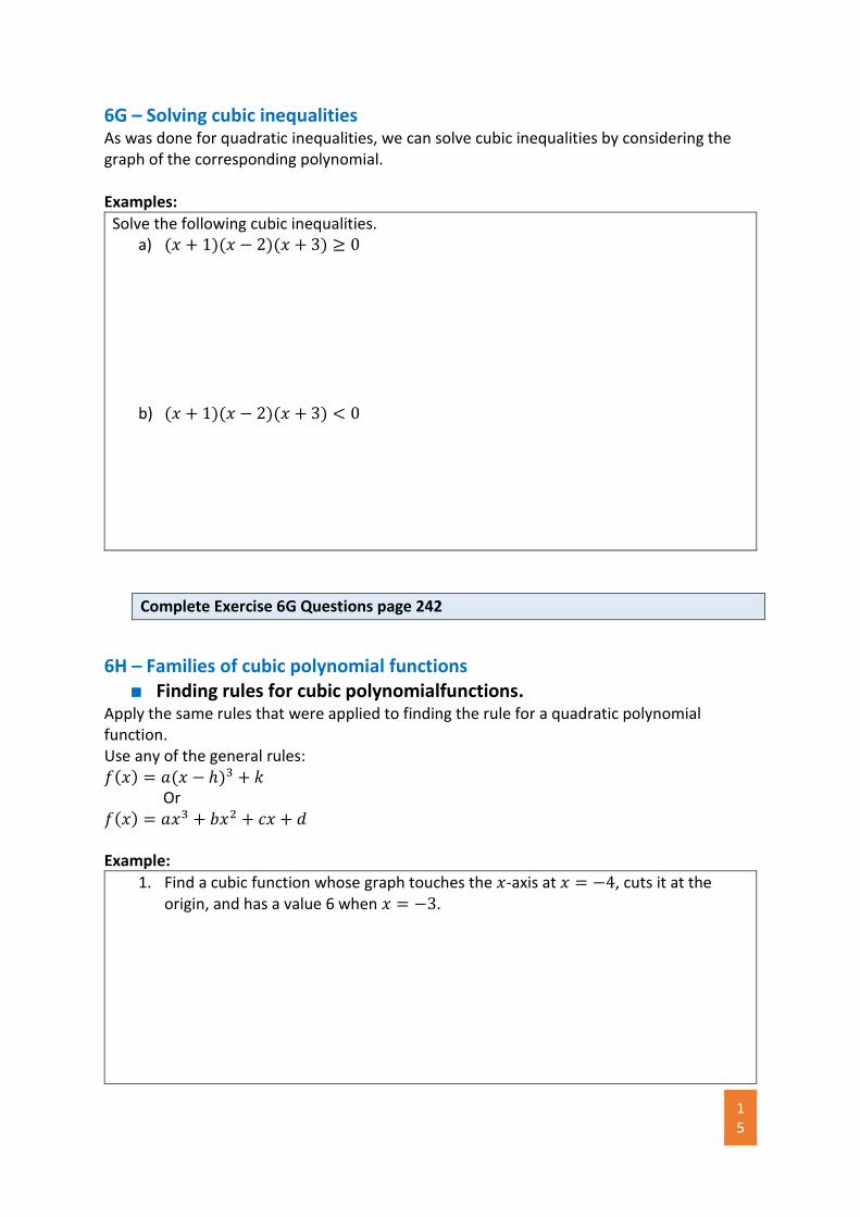
6G – Solving cubic inequalities As was done for quadratic inequalities, we can solve cubic inequalities by considering the graph of the corresponding polynomial. Examples:

Solve the following cubic inequalities. a) (𝑥 + 1)(𝑥 − 2)(𝑥 + 3) ≥ 0

b) (𝑥 + 1)(𝑥 − 2)(𝑥 + 3) < 0

Complete Exercise 6G Questions page 242

6H – Families of cubic polynomial functions ■ Finding rules for cubic polynomialfunctions.

Apply the same rules that were applied to finding the rule for a quadratic polynomial function. Use any of the general rules: 𝑓(𝑥) = 𝑎(𝑥 − ℎ)3 + 𝑘 Or 𝑓(𝑥) = 𝑎𝑥3 + 𝑏𝑥2 + 𝑐𝑥 + 𝑑 Example:

1. Find a cubic function whose graph touches the 𝑥-axis at 𝑥 = −4, cuts it at the origin, and has a value 6 when 𝑥 = −3.

16

2. Find the equation of the following cubic in the form 𝑦 = 𝑎𝑥3 + 𝑏𝑥2.

Complete Exercise 6H Questions page 246

6I – Quartic and other polynomial functions

■ Quartic functions of the form 𝒇(𝒙) = 𝒂(𝒙 − 𝒉)𝟒 + 𝒌 ▪ As with other graphs it has been seen that changing the value of 𝑎 simply narrows or

broadens the graph without changing its fundamental shape.

▪ If 𝑎 < 0, the graph is inverted. ▪ The significant feature of the graph of a quartic of this

form is the turning point. ▪ The turning point of 𝑦 = 𝑥4 is at the origin (0,0). ▪ For the graph of a quartic function of the form

𝒇(𝒙) = 𝒂(𝒙 − 𝒉)𝟒 + 𝒌, the turning point is at (𝒉, 𝒌). When sketching quartic graphs of the form 𝑦 = 𝑎(𝑥 − ℎ)4 + 𝑘, first identify the turning point. To add further detail to the graph, find the 𝑥-axis and 𝑦-axis intercepts. Examples of possible cubic functions and the shape of their graphs.

17

■ Odd and even polynomials Knowing that a function is even or that it is odd is very helpful when sketching its graph.

■ A function 𝑓 is even if 𝑓(−𝑥) = 𝑓(𝑥). This means that the graph is symmetric about the 𝑦-axis. That is, the graph appears the same after reflection in the 𝑦-axis.

■ A function 𝑓 is odd if 𝑓(−𝑥) = −𝑓(𝑥). The graph of an odd function has rotational symmetry with respect to the origin: the graph remains unchanged after rotation of 180° about the origin. A power function is a function 𝑓 with rule 𝑓(𝑥) = 𝑥𝑟 where 𝑟 is a non-zero real number. We will only consider the cases where 𝑟 is a positive integer or 𝑟 ∈ {−2, −1,12,13}.

Even-degree power functions

The functions with rules 𝑓(𝑥) = 𝑥2 and 𝑓(𝑥) = 𝑥4 are examples of even-degree power functions. The following are properties of all even-degree power functions: 𝑓(−𝑥) = (𝑥) for all 𝑥 𝑓(0) = 0

As 𝑥 → ±∞, 𝑦 → ∞. Odd-degree power functions The functions with rules 𝑓(𝑥) = 𝑥3 and 𝑓(𝑥) = 𝑥5are examples of odd-degree power functions. The following are properties of all odd-degree power functions: 𝑓(−𝑥) = −𝑓(𝑥) for all xx 𝑓(0) = 0

As 𝑥 → ∞, 𝑦 → ∞ and

as 𝑥 → −∞, 𝑦 → −∞. Note: if a function has both even and odd powers, it is neither even or odd. Example:

3. State whether the following polynomials is even or odd. a) 𝑓(𝑥) = 3𝑥4 − 𝑥2

18

b) 𝑓(𝑥) = 8𝑥3 + 5𝑥 − 9

4. a) On the same set of axis sketch the graphs of 𝑓(𝑥) = 𝑥4 and 𝑔(𝑥) = 9𝑥2. b) Solve the equation 𝑓(𝑥) = 𝑔(𝑥) c) Solve the inequality 𝑓(𝑥) ≤ 𝑔(𝑥)

Complete Exercise 6I Questions page 252

19

6J – Applications of polynomial functions Textbook examples:

1. A square sheet of tin measures 12 𝑐𝑚 × 12 𝑐𝑚.

Four equal squares of edge 𝑥 cm are cut out of the corners and the sides are turned up to form an open rectangular box. Find:

a) the values of 𝑥 for which the volume is 100 𝑐𝑚3 b) the maximum volume.

Solution The figure shows how it is possible to form many open rectangular boxes with dimensions

12 − 2𝑥, 12 − 2𝑥 and 𝑥.

The volume of the box is

𝑉 = 𝑥(12 − 2𝑥)2, 0 ≤ 𝑥 ≤ 6 which is a cubic model. We complete the solution using a CAS calculator as follows.

2. It is found that 250 metres of the path of a stream can be modelled by a cubic function. The cubic passes through the points (0,0), (100,22), (150,−10), (200,−20).

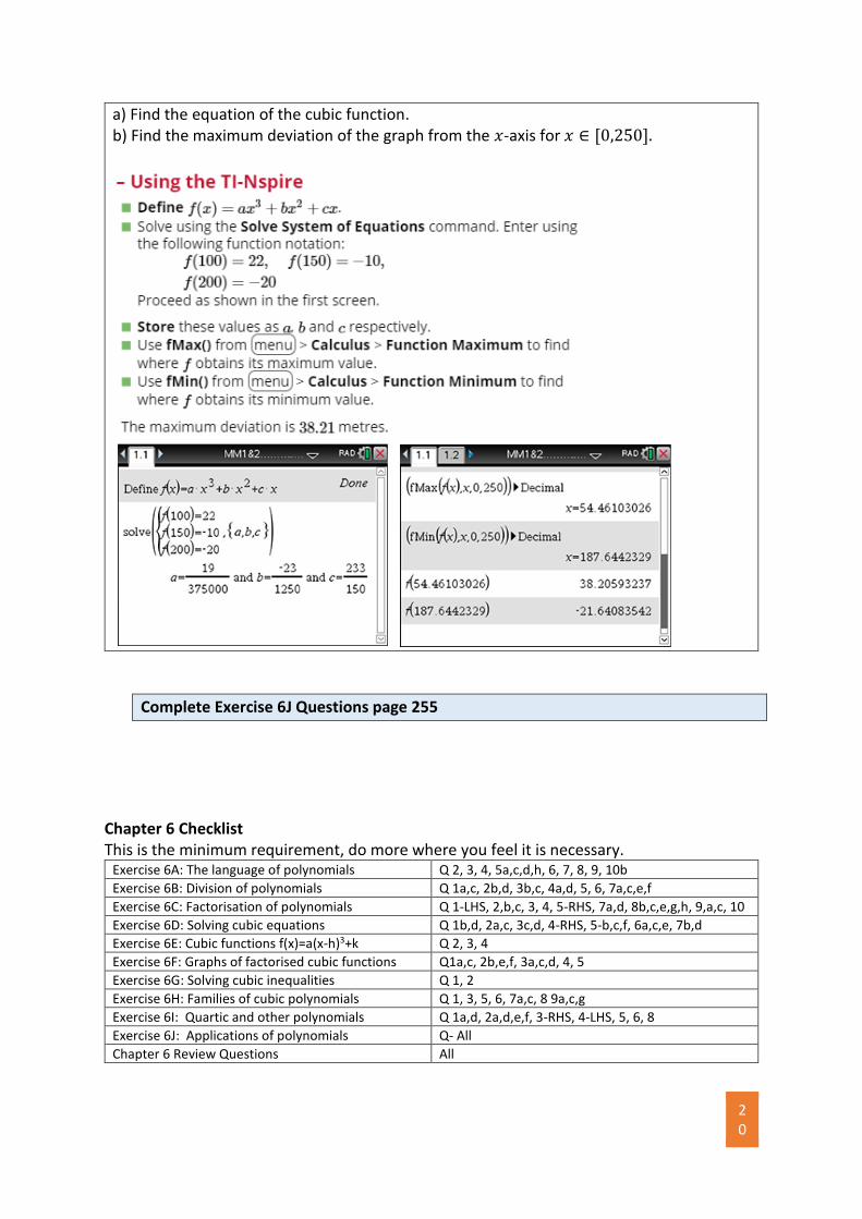
20

a) Find the equation of the cubic function. b) Find the maximum deviation of the graph from the 𝑥-axis for 𝑥 ∈ [0,250].

Complete Exercise 6J Questions page 255

Chapter 6 Checklist This is the minimum requirement, do more where you feel it is necessary.

Exercise 6A: The language of polynomials Q 2, 3, 4, 5a,c,d,h, 6, 7, 8, 9, 10b

Exercise 6B: Division of polynomials Q 1a,c, 2b,d, 3b,c, 4a,d, 5, 6, 7a,c,e,f

Exercise 6C: Factorisation of polynomials Q 1-LHS, 2,b,c, 3, 4, 5-RHS, 7a,d, 8b,c,e,g,h, 9,a,c, 10

Exercise 6D: Solving cubic equations Q 1b,d, 2a,c, 3c,d, 4-RHS, 5-b,c,f, 6a,c,e, 7b,d

Exercise 6E: Cubic functions f(x)=a(x-h)3+k Q 2, 3, 4

Exercise 6F: Graphs of factorised cubic functions Q1a,c, 2b,e,f, 3a,c,d, 4, 5

Exercise 6G: Solving cubic inequalities Q 1, 2

Exercise 6H: Families of cubic polynomials Q 1, 3, 5, 6, 7a,c, 8 9a,c,g

Exercise 6I: Quartic and other polynomials Q 1a,d, 2a,d,e,f, 3-RHS, 4-LHS, 5, 6, 8

Exercise 6J: Applications of polynomials Q- All

Chapter 6 Review Questions All