C H A P T E R 1 2

Unilateral Trade Policy

12.1 Introduction

The economic geography literature is a bit like Hamlet without the Prince. Trade

policy should play the, or at least a, leading role in the literature—or that is what

one might expect since trade barriers are at the very heart of the models and the

literature’s founding fathers are famous for their theoretical trade policy analysis.

Alas, the literature is surprisingly short on trade policy analysis. For example, in

Peter Neary’s excellent overview (Neary 2001), not a single article on trade

policy is referenced.

The reason for this lacuna is uncomplicated. The policy implications implicit

in the standard models do not seem to provide useful insights. As Neary (2001)

remarks:

The key problem is that the policy implications of the basic core–periphery model are

just too stark to be true. The model turns Sartre’s ‘Hell is other people’ on its head:

agglomeration is unambiguously good for you. Because the cost of living is lower in

the core, it is always better to live there than in the periphery, with the level of utility in

a diversified economy lying in between. Faced with multiple equilibria that have a clear

welfare ranking, it is tempting to suggest a role for government in ‘picking equilibria’.

This in turn may encourage a new sub-field of ‘strategic location policy’, perhaps

drawing on fifteen years’ work on strategic trade policy, which, as Brander (1995)

and Neary and Leahy (2000) argue, has produced much interesting theory but no simple

robust rules to guide policy making.’’

Neary concludes with, ‘‘No harm then that FKV are mostly neutral on the applic-

ability of the models to policy.’’

12.1.1 Organization of the Chapter

This chapter begins by taking up the challenge that is implicit in Neary’s analysis

of the CP model’s appropriateness for policy analysis. It does this by first using

our more tractable models (see Part I) to study precisely how ‘strategic location

policy’ works when agglomeration forces are present—that is, how unilateral

protection can lower prices in the protecting nations (what we call the price-

lowering-protection effect). We then introduce a series of enrichments that makes

economic geography models ‘ambiguous enough to be true’, to paraphrase

Neary.

Refuting the price-lowering-protection (PLP) effect, however, is not really

sufficient for showing that economic geography models are suitable tools for

trade policy analysis. Even with the our enrichments, unilateral protection always

fosters industrialization in the sense that a nation can always increase its share of

world industry by imposing a unilateral import barrier. Since unilateral protection

is not generally viewed as a sure-fire route to industrialization in the real world,

the next section explores variants of simple economic geography models in

which trade liberalization can foster industrialization. This involves considera-

tion of imported intermediate goods.

We turn next to the question of why small countries have trouble attracting

industries in which agglomeration forces are important. Of course, the economic

geography models are perfectly suited to answer this question. We focus on the

interplay between domestic and foreign protection, domestic and foreign market

size and comparative advantage.

The last substantive section considers an old chestnut in trade policy analy-

sis—the non-equivalence of tariffs and quotas. As it turns out, these two policies

can have very different effects on the spatial allocation of industry. The final

section provides our concluding remarks and a discussion of related literature.

12.2 Price-Lowering Protection (PLP)

The prime example of the protectionist implications of economic geography

models is the price-lowering effect of protection. In a typical new trade theory

model an increase in unilateral protection lowers the domestic price level.

Venables (1987) first showed this surprising and counter-intuitive effect in a

model without agglomeration forces; Baldwin (1999) shows that the presence

of agglomeration forces serves to strengthen the effect.

This result flies in the face of empirical evidence and common sense, but it

does have clear-cut protectionist implications. In the CP model, for instance, a

nation that erects import barriers (even barriers that generate no tariff revenue or

quota rents) experiences a Pareto welfare improvement in the sense that each

factor-owner gains, the mobile factor gaining both from agglomeration-induced

higher nominal wage and lower prices, while the immobile factor gains only from

the latter. While unilateral protection can be both pricing-lower and welfare-

improving in other models, the PLP effect is novel; see Box 12.1 for details.

To fix ideas, this section first presents a decomposition of PLP that highlights

its source and points to theoretical factors that could reverse it. We then present a

simple model in which the effect can be simply and analytically demonstrated.

12.2.1 Decomposition of Price-Lowering Protection (PLP)

Most economic geography models, including the standard CP model, feature

monopolistic competition where all differentiated varieties enter the representa-

tive consumer’s preferences in a symmetric fashion, and all varieties produced in

a given nation are symmetrically priced. The perfect price index for such prefer-

ences can be expressed as

278 C H A P T E R 1 2

P ¼ P nv½p�; npv½pp�� �

; P1;P2; v’ , 0 ð12:1Þ

where n and n*, are the mass (number) of locally produced and imported vari-

eties; the asterisk indicates foreign variables, as usual. Also, p and p* are the

consumer prices of local and imported goods. The partials of the implicit function

P½ ; � are negative (this reflects the love of variety aspect of the assumed prefer-

ences, and the derivative of n½ � is negative, so at any price rise P is raised. The

impact of unilateral protection on such a price index is

dP

dt¼ P1 nv’

dp

dt1 v

dn

dt

� �1 P2 npv’

dpp

dt1 ppv

dnp

dt

!ð12:2Þ

where t measures the level of home protection, and P1 and P2 are the partials

of P½ ; � with respect to the first and second arguments, respectively. Since

protection can alter factor prices and market structure, the derivatives in this

expression are, in general, quite complex. Intuition, however, is served by a

few of the simplifying assumptions commonly made in the economic geogra-

phy literature.

If varieties are symmetric across nations as well as within nations, we have

that P1 ¼ P2 and for brevity, we write P1 ¼ P2 as P 0. Economic geography

models often work with frameworks where mill pricing is optimal since this

assumption eliminates pro-competitive effects; the result is that p is propor-

tional to w and p* is proportional to w*t , where w and w* are the home and

foreign wage rates. In some economic geography models, a change in t will

affect w and w*, however, if we start at the symmetric point with symmetric

nations, all effects will be equal and opposite; for example, dw=dt ¼ 2dw*=dt

starting from a point where w ¼ w* and t ¼ t*. Finally, it proves convenient

to write n and n* in terms of shares and the global number of varieties, viz.

n ¼ snnw and n* ¼ ð1 2 snÞnw. Using these assumptions and evaluating (12.2)

at the symmetric point yields

U N I L A T E R A L T R A D E P O L I C Y

BOX 12.1 PRICE LOWERING EFFECTS IN NEOCLASSICAL TRADE MODELS

In a neoclassical trade model (e.g. Ricardian or Heckscher–Ohlin), a sufficiently

small tariff can induce a welfare-improving price reduction in any nation that is not

atomistic. This so-called optimal tariff reduces the home nation’s demand for

imports and this in turn lowers the international price for its imports. This differs

greatly from the PLP effect discussed in this chapter. The classical ‘optimal tariff’

works by pushing down the border price and indeed it requires the domestic price of

imports to rise. For this reason, the optimal tariff argument does not apply to

‘frictional’ trade barriers such as unilateral changes in iceberg trade costs. To put

it differently, the optimal-tariff gain stems from the fact that part of the tariff’s

incidence falls on foreigners, it therefore only works for trade barriers that generate

domestic revenue; the ‘optimal tariff’ is just a tricky way of taxing foreigners.

279

dP

dt¼ 2nwð2P’Þ v½p�2 v½pp�

ÿ � dsn

dt1

nw

2ð2P’Þ 2v’½p�

dp

dt2 v’½pp�

dpp

dt

!

22P’

2

� �v½pp�1 v½pp�ÿ � dnw

dtð12:3Þ

DISCUSSION

Equation (12.3) decomposes the price-index impact into three parts. The first

right-hand term reflects what we called the ‘location effect’ in Chapter 10. The

idea here is that p* . p with mill pricing (the price of imported varieties includes

trade costs), so v½p*� , v½p*� and this means that if protection yields inward

delocation—that is, dsn=dt . 0—then protection tends to lower the price

index. More heuristically, the location effect simply reflects the fact that the

index tends to falls when a large fraction of varieties are produced locally

since this allows home consumers to avoid the trade costs on a wider range of

goods.

The second effect—which corresponds to the ‘trade price effect’ in Chapter

10—shows how a protection-induced change in p and p* affects the price index.

Note that since the (2P 0) and (2n 0) terms are positive, increases in either p or p*

tend to raise P. We normally expect the direct effect to raise P for two reasons.

First, an increase in trade costs t will raise p* automatically given mill pricing,

and second, general equilibrium factor price effects are likely to result in a rise in

p (since the protection boosts demand for domestic output and thus factors), or at

least no change.

The final effect—captured by the third right-hand term—is the famous

variety effect. Given that n . 0 and P 0 , 0, an increase in nw lowers the

price index. We note that most economic geography models (including the

CP model) make assumptions that render the total number of varieties, that is,

nw, invariant to trade barriers. For such models, the third term drops out

leaving us with two effects, the direct effect, which tends to raise P, and

the delocation effect, which tends to lower it. In short, PLP only works in

mainstream economic geography models, when the ‘delocation elasticity’ is

sufficiently high. Specifically, when

dsn

dt.

1

2

v 0½p�dp

dt1 v 0½pp�

dpp

dtv½p�2 v½pp�

ð12:4Þ

To summarize this analysis, we write the following result.

Result 12.1. Unilateral protection can lower prices in standard economic

geography models since the direct price-raising impact of protection may

be more than offset by the delocation of firms into the home market. PLP

only works when the ‘delocation elasticity’ is sufficiently high.

280 C H A P T E R 1 2

12.2.2 Stark Results in Simple Models: PLP in the FC and CC Models

In the model with which Venables (1987) first showed the PLP effect, the elas-

ticity of delocation is very high. This section shows that this is also true of simple

economic geography models by reproducing and analysing the PLP using simple

models. In the models we employ—the FC model of Chapter 3 and the CC model

of Chapter 6—the global number of varieties is invariant to trade policy, just as it

is in the CP model and in Venables (1987). We start with the FC models where

unilateral protection leads to gradual delocation, postponing issues of cata-

strophic agglomeration to the subsequent section.

PLP IN THE FC MODEL

The FC model that we employ is described at length in Chapter 3, so here we just

remind readers of the key assumptions and reproduce the equilibrium conditions.

The basic set-up consists of two nations, home and foreign (in the trade chapters

we use home and foreign instead of north and south, with home taking north’s

notation), two factors (labour, L, and physical capital, K) and two sectors (M and

A). Physical capital can move freely between nations, but capital owners cannot,

so all K reward is repatriated to the country of origin. Industrial and agricultural

goods are traded. Trade in A is costless. Industrial trade is impeded by frictional

(iceberg) import barriers such that 1 1 t $ 1 units of a good must be shipped in

order to sell one unit abroad (t is the tariff equivalent of the trade costs). Countries

have identical preferences and technology. To keep things simple, we assume

that nations have identical endowments, but to allow for unilateral protection, we

suppose that they have potentially different iceberg trade costs for industrial

imports. Preferences of the representative consumer comprise the usual Cobb–

Douglas nest of a CES aggregate of industrial varieties and consumption of the A

good. The representative consumer owns the entire nation’s L and K and his/her

income (and expenditure) equals wL 1 pK (there is no tariff revenue with

iceberg barriers).

Combing free trade and perfect competition in A, with our standard normal-

izations, we get pA ¼ p*A ¼ w ¼ w* ¼ 1.1 Also, with ‘mill pricing’ in the M

sector, home M firms charge p ¼ 1 for local sales and p ¼ t for export sales.

Using this, the operating profit of a typical northern industrial firm reduces to

p ¼ BbEw

Kw; B ;

sE

D1

fpspE

Dp ; D ; sn 1 fspn; Dp ; fpsn 1 sp

n; b ;m

s

ð12:5Þ

where f ; t12s and f* ; t*12s are measures of north’s and south’s openness

(i.e. t 2 1 is the tariff equivalent of the frictional barriers faced by southern firms

selling to the north, and t* 2 1 is the corresponding value for northern exports to

the south). The rest of the notation is standard (Ew and Kw ¼ nw are world

U N I L A T E R A L T R A D E P O L I C Y

1 We assume that the no-specialization condition holds; m , 1=2 is sufficient (see Chapter 3 for

details).

281

expenditure and world capital stock, Kw is normalized to unity, sE is the north’s

share of Ew, and sn is the share of nw made in the north, and finally sn* equals

1 2 sn). As usual, B measures the extent to which a northern variety’s sales

exceed the world average per variety sales (which is mEw=Kw), and thus the extent

to which p exceeds the world average operating profit (which is bLw=Kwð1 2 bÞ

as Chapter 3 shows in detail). Similar foreign expressions hold with foreign

variables denoted with an asterisk.

Capital movements are assumed to be costless, so capital moves and thus n ¼

sn and n* ¼ 1 2 sn adjust until p ¼ p*.2 This has several important implications.

First, it means that each unit of capital earns the global average reward

bLw=Kwð1 2 bÞ and, importantly, this does not vary with the level of protection

or the spatial allocation of industry. For simplicity, we work with two nations that

have identical endowments, and since p ’s are equalized in equilibrium and

remitted, home’s share of world expenditure, sE, never varies and by symmetry

it equals 1/2.

With sE ¼ 1=2, the location condition p ¼ p* can be solved for sn to yield a

closed-form solution for the equilibrium spatial distribution of industry and its

dependence on openness, that is,

sn ¼1

21

1

2

fp 2 f

ð1 2 fÞð1 2 fpÞð12:6Þ

This is the model’s key equilibrium condition. Plainly, with symmetric protec-

tion, industry would be evenly divided between the two regions regardless of the

level of trade freeness. Observe that raising home protection unambiguously

raises home’s share of industry and raising foreign protection unambiguously

lowers it. Specifically, from (12.6), the delocation derivatives, dsn=dt and dsn=df,

in this model evaluated at symmetric trade freeness are

dsn

dt¼ðs 2 1Þt2s

2ð1 2 t12sÞ2. 0;

dsn

df¼

21

2ð1 2 fÞ2ð12:7Þ

This gets arbitrarily large as the level of freeness increases. This is summarized in

the following result.

Result 12.2. Unilateral protection raises a nation’s share of global indus-

try in the FC model. The size of this ‘delocation derivative’ rises with the

initial level of openness.

The increasing sensitivity of industrial location to asymmetric protection should

be thought of as a corollary to the ‘home-market magnification effect’ discussed

in Part I.

UNILATERAL PROTECTION IN THE SYMMETRIC FC MODEL

Here, we focus on home unilateral protection and its impact on the home price

index, namely

282 C H A P T E R 1 2

2 We focus on interior equilibria here; see Chapter 3 for an analysis of core–periphery outcomes.

P ¼ ðnwDÞ2a; a ;m

s 2 1. 0 ð12:8Þ

since pA ¼ 1 and both home and foreign varieties are priced at unity for local

sales (see Chapter 3 for a detailed derivation of this ‘perfect’ price index). Plug-

ging (12.6) into the definition of D and differentiating, we get

dP=df

P¼ 2

a

D1 2 sn 1 ð1 2 fÞ

dsn

df

� �¼ a

fp

1 2 ffp

!. 0 ð12:9Þ

The first term in the large parentheses in (12.9) is the direct effect of liberalization

on the price index. The second term is the location effect. The second expression

follows from the first after evaluating dsn=df with (12.7) and the equilibrium

value of sn with (12.6). As inspection reveals, dP=df is always positive (as

indicate by the inequality), so unilateral liberalization always raises the liberal-

izer’s price index. The reason, of course, is that the delocation derivative dsn/df

is so large. This is summarized in the following result.

Result 12.3. Unilateral protection lowers the protecting nation’s price

index in the symmetric FC model.

Discussion. Three observations can be made concerning this result. First, PLP

stems entirely from protection-induced relocation of industrial firms. To see this

observe from (12.9) that the magnitude of the effect rises with manufactures’

expenditure share, m , and falls as the M varieties become better substitutes since

a ; m=ðs 2 1Þ. In the limit, when varieties are perfectly substitutable, that is,

s ¼ 1, or home consumers spend nothing on M, that is, m ¼ 0, policy-induced

delocation has no price implications. The same point can be seen by noting that if

dsn=df were zero, liberalization would lower prices.

Second, the gain from unilateral protection rises as the initial overall level of

protection falls. For instance, suppose the two nations start with f ¼ f* and

home is considering a marginal decrease in its trade freeness. By inspection of

(12.9), the size of the welfare gain from such protection gets very large as the

initial level of symmetric freeness approaches costless trade. The reason, of

course, is that when trade costs are almost zero, firms are almost indifferent to

their location so any small locational advantage has an outsized impact on loca-

tion of industry. Thus, in some sense, the temptation for a nation to ‘cheat’ on a

reciprocal trade liberalization increases as the depth of integration rises. This so-

called magnification effect of globalization (Baldwin 2000) may help explain

why deep integration schemes—such as the EU and the EEA—seems to require

much stronger trans-national mechanisms for surveillance, enforcement and

adjudication than free trade areas, such as NAFTA and EFTA. To spotlight

this, we write the following result.

Result 12.4. The welfare gains from a slight, unilateral increase in protec-

tion are larger when starting from a position of initially liberal trade. Thus,

a nation’s incentive to ‘cheat’ is higher, not lower as intuition might

suggest, when trade is quite free to begin with.

U N I L A T E R A L T R A D E P O L I C Y 283

Third, if we had worked with an economic geography model with more powerful

agglomeration forces, the amount of industry that would delocate in response to

unilateral protection would be even greater. (Recall from Part I that the FC model

is the economic geography model with the weakest agglomeration forces.)

RETALIATION

Delocation in this model is a zero sum game and since a reduction in the share of

varieties that are produced locally always harms a nation, home’s unilateral

protection harms foreigners. To see this more carefully, note that protection

has no impact on E or E* so differentiating the foreign indirect utility function,

V* ¼ E*=P*, yields ðdV*=dfÞ=V* ¼ aðdD*=dfÞ=D*, where

dDp=df

Dp ¼ð1 2 fpÞ

ð1 2 fÞð1 2 ffpÞð12:10Þ

Thus, foreigners lose when home unilaterally raises its level of protection (i.e.

when df , 0). Again, the size of the welfare loss rises as the initial level of

symmetric trade freeness rises.

Given this win–lose aspect of unilateral protection, foreigners are unlikely to

view home protection benignly. Indeed, if the two nations play a Nash protection

game, the only equilibrium is prohibitive barriers. The point is easily made.

Taking the indirect utility function (i.e. V ¼ E=P) as the objective of the home

government, the home government’s first order condition can be written as

dV =df

V¼

2afp

1 2 ffp # 0; f $ 0; w:c:s: ð12:11Þ

where w.c.s. stands for ‘with complementary slackness’. By symmetry, we can

solve for the Nash equilibrium level of freeness by imposing symmetry. Employ-

ing fne ¼ f ¼ f* in (12.10), we get fne ¼ 0 is the only solution. Thus, we have

he following result.

Result 12.5. If nations play Nash in their level of openness, the only

equilibrium entails prohibitive trade barriers.

This extreme result is intuitively obvious. Any delocation of firms to home is

welfare improving. The optimal home policy is thus to set home trade free-

ness, f , low enough to ensure that all M firms are in the home. From (12.6),

this holds for any f that is more protectionist than ð2f*2 1Þ=f*, subject to

0 # f. Of course, a symmetric full relocation condition holds for foreigners,

so both governments would be driven to setting the protection at prohibitive

levels.

What all this goes to say is that PLP acts very much like an extreme form of the

terms-of-trade-shifting argument for tariff protection in Walrasian trade models.

Thus, just as in the old literature, unilateral protection engages governments in a

prisoners’ dilemma; reciprocal free trade may be the best realistic option even if

unilateral free trade is not.

284 C H A P T E R 1 2

CATASTROPHIC PLP EFFECT: THE CC MODEL

The PLP effect illustrated above works in a smooth way, but how does it work in

a model where catastrophic agglomeration is a possibility? As Chapter 6 showed,

it is simple to add demand-linked circular causality to the FC model. The result,

the CC model, yields a closed-form solution for the spatial division of industry in

a model where agglomeration can collapse catastrophically.

The two key expressions for the CC model (see Chapter 6 for derivations and

motivation) are

sn ¼ð1 2 fpfÞsE

ð1 2 fÞð1 2 fpÞ2

f

1 2 f; sE ¼ ð1 2 bÞsL 1 bsn ð12:12Þ

where b ; br=ðr 1 dÞ and b ; m=s. The first expression, which is identical to the

corresponding condition for the FC model, shows that expenditure shifting leads

to production shifting in the CC model. The second expression shows that, unlike

the FC model, production shifting also leads to expenditure shifting in the CC

model (in the FC model, sE is fixed parametrically).

The interior equilibrium becomes catastrophically unstable when the slope of

the first expression with respect to sE exceeds the inverse of the slope of the second

expression with respect to sn. The reason is that for such levels of openness, a shock

to firm location sparks a self-reinforcing cycle of expenditure shifting and produc-

tion shifting that results in all industry being located in one nation.

The easiest way to characterize the collapse is to find the closed-form solution

for the north’s share of industry (we do this by plugging the second expression in

(12.12) into the first), and check when a slight increase in northern protection

would induce all industry to decamp to the north. The result of the closed-form

solution for sn with asymmetric protection, but symmetric endowments is

sn ¼1

2

1 1 ffp 2 2f 2 ð1 2 ffpÞb

ð1 2 fÞð1 2 fpÞ2 ð1 2 ffpÞbð12:13Þ

To complete the analysis, we start out with identical levels of protection, so

f ¼ f*, and parameterize the north’s unilateral protection by introducing the

parameter 1 ; f=f* # 1. Then, we differentiate the resulting expression for sn

with respect to 1 and evaluate the derivative as 1 ¼ 1. The result is

dsn

d1¼

2f=2

ð1 2 fÞ2 2 ð1 2 f2Þbð12:14Þ

By inspection, this ‘delocation derivative’ is infinite when f ¼ ð1 2 bÞ=ð1 1 bÞ.

This critical value is none other than the break point of the symmetric CC model.

This is summarized in the following result.

Result 12.6. In the CC model, which allows for self-reinforcing agglom-

eration, that is, circular causality, a slight unilateral increase in protection

by one nation, can cause a catastrophic agglomeration of industry into the

protecting nation when the level of openness is near the break point. This

massive delocation will lower prices and raise welfare in the protecting

nation, and do the opposite in the other nation.

U N I L A T E R A L T R A D E P O L I C Y 285

12.2.3 What’s Wrong with this Picture?

In the model described above, import substitution is always a winning policy in

the sense that unilateral protection is a sure-fire route to promoting industrializa-

tion and the national interest. Putting the conclusion in this way brings at least

three qualifications to mind.

First, relocation of industrial activity is expensive. While the notion of costly

relocation is perfectly reasonable, parsimony has led standard economic geogra-

phy models to ignore this important facet of the real world. As it turns out,

including it has important implications.

Second, import substitution is an attempt to boost an industry (which amounts

to forcing relocation in this economic geography model) by creating a sheltered

market for firms. If the protected nation is very small, such policies may be

ultimately fruitless; even near-prohibitive import barriers may result in no relo-

cation.

The third qualification is that comparative advantage matters. The standard

economic geography models ignore comparative advantage for simplicity.

However, by making firms a priori indifferent to location on the supply side,

the standard model stacks the odds in favour of PLP by making dramatic deloca-

tion easier. While such a simplification is reasonable for many purposes, it is

clearly inappropriate for trade policy analysis. For instance, when thinking about

why import substitution failed in Latin America, it is impossible not to point to

the fact that these nations had massive comparative disadvantages in many of the

industries they were trying to foster.

We turn now to extending the model to capture the first of these qualifications.

We do so by introducing the concept of relocation barriers, that is, barriers to

capital movement.

12.2.4 Ambiguity with Relocation Barriers

It is costly to relocate production abroad. This section shows that allowing for this

natural factor can reverse the stark PLP result. For simplicity, we consider a ‘per

unit’ relocation cost, that is, a relocation cost that is the same for all firms and is

unaffected by the amount of relocation that has occurred. A key insight in this

section is that the stark protectionist implications of PLP are not intrinsic to

economic geography models. Rather, they stem in a large part from the simplify-

ing assumption that moving firms is costless, but moving goods is costly.

FLAT RELOCATION COSTS: DISCONTINUOUS PLP

Some relocation costs are natural, but some are man-made. Natural costs include

linguist, cultural and climatic differences between a firm’s host and home nations,

coordination costs over distance, etc. The list of man-made barriers is much

longer. Nations, especially developing nations, have many policies that implicitly

make it difficult for foreign firms to produce locally. For instance, foreign firms

286 C H A P T E R 1 2

may require a large and uncertain number of permits in order to do business. Or

they may be made to strictly adhere to local tax, labour, heath and environmental

laws, while local firms may be allowed to skirt them. Foreign firms may also be

systematically subject to greater pressures to directly or indirectly pay off local

officials. Finally, foreign firms may have much higher costs of acquiring infor-

mation about local production conditions, legal systems and local consumers.

Clearly, the most satisfactory route would be to provide micro-foundations for

each of the factors separately. Doing so, however, would take us too far afield.

To illustrate the importance of relocation costs as clearly as possible, we

continue to work with the symmetric FC model, but we now allow for a reloca-

tion cost. Specifically, we assume that a firm relocating from one nation to

another pays a proportional cost of 1 2 k, where 0 # k # 1 is a measure of

the freeness of capital’s mobility. That is, k ¼ 1 indicates costless capital mobi-

lity and k ¼ 0 indicates zero (infinitely costly) capital mobility. (Note that both

trade freeness and capital freeness are parameterized such that 1 is perfectly free

and 0 is perfectly closed.) Importantly, we assume that this is a one-time cost and

focus on situations where it has already been incurred so that the relocation cost

has no impact on current earnings.3

The No-Delocation Band. Begin by considering what would happen to p and

p * if same-size nations had different trade barriers, but relocation was

forbidden.4 As usual, higher home protection makes home more attractive in

the sense that p . p* when sn is held at 1/2. Now given this difference, would

firms relocate from foreign to home if they faced relocation costs? Plainly,

relocation would only occur if relocation were sufficiently cheap, that is, if the

relocation costs 1 2 k were sufficiently small. Specifically, firms would move

only if pk . p* (evaluated at sn ¼ 1=2). This is captured by the following

inequalities that hold with complementary slackness5

f , fp ) pk # pp; sn $1

2; w:c:s:

f . fp ) ppk # p; sn #1

2; w:c:s: ð12:15Þ

The first of these applies when home protection (i.e. f , f*) creates an incipient

inflow of firms/capital. If any foreign firms do relocate to home—which, given

the initial symmetry, is tantamount to sn . 1=2—they will do so up to the point

where kp ¼ p* with k # 1. The second equation covers the mirror-image case

where foreign is more protectionist.

U N I L A T E R A L T R A D E P O L I C Y

3 We have worked out an alternative model—the melting capital model—where k represents a flow

cost. The results are broadly similar, but the analysis is more complex since regional expenditure

levels depend upon capital flows.4 This is identical to the short-run analysis in Chapter 3.5 Here, we assume, as usual in the economic geography literature, that firms are myopic. If they

were forward looking, the condition would compare the present value of the p difference to the one-

off cost. We could repeat all the analysis using rk to reflect this; nothing important would change.

287

To characterize the range of f where delocation is not worthwhile (so sn

remains at 1/2), we solve kp ¼ p* and p ¼ kp* for the critical levels of f

using (12.5). We refer to this as the ‘no-delocation band’, or ‘hysteresis band’.

The task, however, is complicated by the fact that even though sn remains

unchanged in the band, sE changes since p does not equal p * with f – f*.

For example, starting at full symmetry, home protection raises p and lower

p *, even if sE stayed at 1/2. This increase in home earning power, however,

also raises sE and this in turn leads to a further increase in p and a decrease in

p *. In other words, the model with relocation costs displays a form of demand-

linkage that was not present above.

To deal with this demand link, we solve sE ¼ E=Ew for sE (with sn fixed since

we are in the band) to get

sE ¼1

2

� �ð1 1 fÞ½ð1 1 fpÞb 2 ð1 1 fpÞ�

ð1 2 ffpÞb 2 ð1 1 fpÞð1 1 fÞð12:16Þ

A demand linkage of sorts can be seen since sE rises as home protection increases.

For example, dsE/df equals 2b=½2ð1 1 fÞð1 2 b 1 fð1 1 bÞ� , 0 when evalu-

ated at the symmetry point. As long as protection levels stay within the band, the

change in relative market sizes has no impact on location of industry, so inside

the band this is just half of the demand-linked circular causality that exists in

operation (see Chapters 3 and 4 for details).

Using (12.16) in (12.5) and its foreign analogue, we can implicitly define the

limits of the band with symmetric-sized nations with the equations kp ¼ p* and

p ¼ kp*. Solving these, we find the range of f for which sn ¼ 1=2 given f * and

k . This is the no-delocation band, namely

flower ¼2kfp 2 ð1 2 bÞð1 2 kÞ

2 1 ð1 1 bÞð1 2 kÞfp ; fupper ¼2fp 1 ð1 2 bÞð1 2 kÞ

2k 2 ð1 1 bÞð1 2 kÞfp ð12:17Þ

For values of f within this range, the delocation elasticity is zero. Note that the

band widens as f * increases since the gain from asymmetric protection

diminishes as the overall level of barriers falls. Figure 12.1 shows that the

band partitions protection space into three regions. Inside the band, no delocation

occurs, but on either side, home protection will increase sn. The figure also

illustrates the point that the band narrows as delocation costs fall; that is, the

degree of capital mobility, k , rises.

The Price Implications. In the no-delocation band, unilateral protection has the

usual price-rising impact on the price index (since dsn=df ¼ 0 inside the band,

only the ‘direct effect’ operates). For example, if f * remains constant and home

lowers f starting from f ¼ f*, the home price index rises as f approaches

f lower. The reason is that lowering f raises the home price index by increasing

the price of imported varieties without affecting the price of local varieties or the

number of varieties produced locally.

288 C H A P T E R 1 2

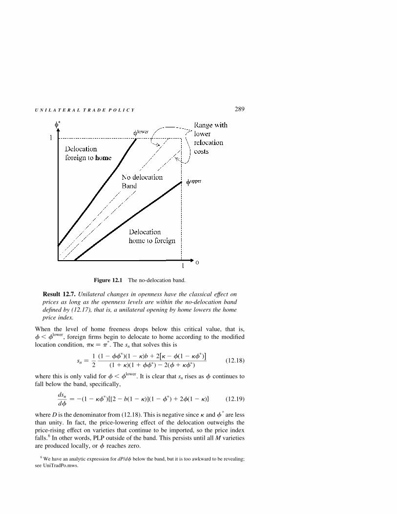
Result 12.7. Unilateral changes in openness have the classical effect on

prices as long as the openness levels are within the no-delocation band

defined by (12.17), that is, a unilateral opening by home lowers the home

price index.

When the level of home freeness drops below this critical value, that is,

f , flower, foreign firms begin to delocate to home according to the modified

location condition, pk ¼ p*. The sn that solves this is

sn ¼1

2

ð1 2 ffpÞð1 2 kÞb 1 2 k 2 fð1 2 kfpÞ� �

ð1 1 kÞð1 1 ffpÞ2 2ðf 1 kfpÞð12:18Þ

where this is only valid for f , flower. It is clear that sn rises as f continues to

fall below the band, specifically,

dsn

df¼ 2ð1 2 kfpÞf½2 2 bð1 2 kÞ�ð1 2 fpÞ1 2fð1 2 kÞg ð12:19Þ

where D is the denominator from (12.18). This is negative since k and f * are less

than unity. In fact, the price-lowering effect of the delocation outweighs the

price-rising effect on varieties that continue to be imported, so the price index

falls.6 In other words, PLP outside of the band. This persists until all M varieties

are produced locally, or f reaches zero.

U N I L A T E R A L T R A D E P O L I C Y

Figure 12.1 The no-delocation band.

6 We have an analytic expression for dP/df below the band, but it is too awkward to be revealing;

see UniTradPo.mws.

289

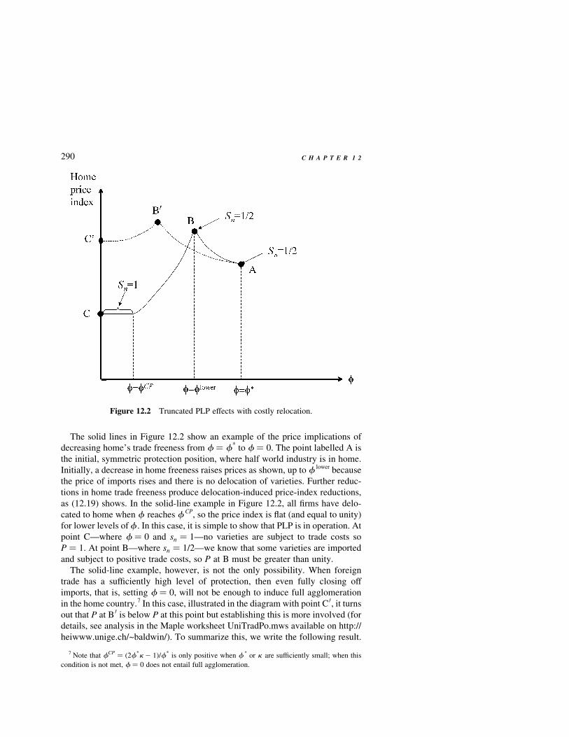
The solid lines in Figure 12.2 show an example of the price implications of

decreasing home’s trade freeness from f ¼ f* to f ¼ 0. The point labelled A is

the initial, symmetric protection position, where half world industry is in home.

Initially, a decrease in home freeness raises prices as shown, up to f lower because

the price of imports rises and there is no delocation of varieties. Further reduc-

tions in home trade freeness produce delocation-induced price-index reductions,

as (12.19) shows. In the solid-line example in Figure 12.2, all firms have delo-

cated to home when f reaches f CP, so the price index is flat (and equal to unity)

for lower levels off . In this case, it is simple to show that PLP is in operation. At

point C—where f ¼ 0 and sn ¼ 1—no varieties are subject to trade costs so

P ¼ 1. At point B—where sn ¼ 1=2—we know that some varieties are imported

and subject to positive trade costs, so P at B must be greater than unity.

The solid-line example, however, is not the only possibility. When foreign

trade has a sufficiently high level of protection, then even fully closing off

imports, that is, setting f ¼ 0, will not be enough to induce full agglomeration

in the home country.7 In this case, illustrated in the diagram with point C 0, it turns

out that P at B 0 is below P at this point but establishing this is more involved (for

details, see analysis in the Maple worksheet UniTradPo.mws available on http://

heiwww.unige.ch/~baldwin/). To summarize this, we write the following result.

290 C H A P T E R 1 2

Figure 12.2 Truncated PLP effects with costly relocation.

7 Note that fCP ¼ ð2f*k 2 1Þ=f* is only positive when f * or k are sufficiently small; when this

condition is not met, f ¼ 0 does not entail full agglomeration.

Result 12.8. Unilateral reductions in openness lead to lower prices in the

protecting nation when the protecting nation’s level of openness is below

the no-delocation band defined by (12.17).

Truncated and Overall PLP. The fact that the home price index falls when it

raises its level of protection beyond the no-delocation band can be thought of as a

‘truncated’ PLP effect. A natural question, however, is whether home prices rise

or fall when home moves its level of openness from the symmetric position,

where f ¼ f*, to the extreme position where f ¼ 0. In other words, would

home see its prices fall if it were to shut off all imports of manufactured

varieties? If the answer is no, home will clearly be better off staying with

symmetric protection. As we shall see, the answer depends upon k , f * and b.

To study this, we define a test for what we call the ‘overall PLP’ effect, that is,

a test for whether a shift from symmetric protection to prohibitive protection

lowers home’s price index. Maintaining our assumption of symmetric sized

nations, the test is8

b 1 kð2 2 bÞ

2½kð1 2 fpÞ1 1 2 kfp�.

1 1 fp

2ð12:20Þ

where the left-hand side is D ¼ sn 1 fð1 2 snÞwhere sn is from (12.18) evaluated

at f ¼ 0, and the right-hand side is D ¼ sn 1 fð1 2 snÞ evaluated at sn ¼ 1=2 and

symmetric openness levels.

To characterize the constellation of parameters where the overall PLP

effect holds, we first point out that if capital movement is perfectly free,

that is, k ¼ 1, then the PLP test is positive (??please check) since we are in

the standard FC model where PLP holds (see Result 12.3). If capital move-

ments are perfectly restricted, that is, k ¼ 0, then the PLP effect does not

hold; this is an implication of Result 12.7 and the fact that the entire

openness space is inside the no-delocation band when capital movement

is prohibitively expensive. To make a more precise statement about how

free capital movements must be to yield the PLP result, we impose an

equality sign on (12.20) and solve for k . This tells us that when capital

movements are freer than k 0, where k 0 ¼ ð1 2 f 2 bÞ=ð1 2 f 2 b 1 2f2Þ,

the PLP result holds. This is summarized in the following result.

Result 12.9. If capital movements are sufficiently costly, unilateral protec-

tion raises the domestic price index and thus lowers welfare in the protect-

ing nation. The critical level of capital movement cost is lower when the

other nation has very low trade barriers and agglomeration forces (as

measured by b ¼ m=s) are strong.

This result is quite intuitive. When foreign is very open to trade, firms find it

cheap to supply foreign consumers from the home country and thus they are

easily induced into moving to the home nation. The impact of agglomeration

U N I L A T E R A L T R A D E P O L I C Y

8 The ratio of price indices equals the ratio in the expression raised to the power of m=ð1 2 sÞ, but

since this is compared to unity, we can dispense with the power.

291

forces is similarly straightforward. When agglomeration forces are strong, delo-

cation of firms from foreign to home are self-reinforcing and so are more easily

induced.

12.2.5 Political Economy of Protection with Entry Barriers

In the real world, import substitution policies typically end up sustaining a few,

poorly run and economically inefficient firms that are—not coincidentally—

controlled by politically powerful groups. This section considers political econ-

omy forces that help make sense of this common outcome. In short, we suggest

that import protection creates conditions in which entry barriers become very

attractive to domestic industry. The reasoning is based on Baldwin and Robert-

Nicoud (2002).

We continue to work with the previous section’s model, namely the FC model

with costly capital relocation. To illustrate the reasoning, consider two extreme

policy combinations—capital market barriers without unilateral protection, and

unilateral trade protection without capital market barriers. Under the first combi-

nation (f ¼ f* and k , 1), relocation costs have absolutely no impact; starting

at equilibrium, specifically at p ¼ p*, no relocation would occur in any case so

the costs are irrelevant. The important point is that home capital owners would

have no incentive to lobby for entry restrictions if there were no protection.

Under the second combination (f , f* and k ¼ 1), the unilateral reduction in

home trade freeness would tend to attract foreign firms and since firms can move

costlessly, the location condition implies that new firms enter until the condition

p ¼ p* is restored. We have seen that the equalized reward to capital p ¼ p* is

invariant to trade freeness and the spatial allocation of firms.9 The key point here

is that because the reward to capital is completely unaffected by protection,

lobbying for protection has no effects on capital owners’ incomes and thus

industry would have no incentive to lobby.10

To summarize these results we write the following result.

Result 12.10. If capital movements are costless, industry has no incentive

to lobby for protection since foreign entry continues until the reward to

capital is force back down to the pre-protection level. Moreover, if the

home market is not more protected than the foreign market (i.e. home

and foreign have the same levels of openness), there is no gain from

lobbying for capital flow restrictions since no capital will flow in any

case.

However, as we saw above, the combination of unilateral protection and entry

barriers does raise the earnings of local capital owners. Thus, protection creates

an incentive for local capitalist/industrialists to lobby for relocation barriers, and

vice versa. This suggests the following sequence of events. A government deci-

292 C H A P T E R 1 2

9 The typical operating profit is invariant to trade policy and in fact it equals bLw=ð1 2 bÞnw, where

b ¼ m=s and both nw ¼ Kw and Lw are fixed by endowments.10 This line of reasoning is pursued in greater depth in Baldwin and Robert-Nicoud (2002).

des to impose unilateral protection, justified perhaps under the rubric of import

substitution. Once the trade barriers are in place, restrictions on capital inflows

become a source of gain for local capital owners.We can go somewhat further and

argue that the utility levels, as well as the incomes, of capital owners be raised by

a package of protection and entry barriers under certain circumstances. The

reason is that for a fairly wide range of parameter values, protection-cum-reloca-

tion costs can raise the real income of K owners. This is obviously true if the

package lowers the local price index (since k , 1 raises their nominal earnings),

but it can also hold in some cases where the package raises local prices.

To look at this more closely, we take the real reward to local K owners as the

objective function of the K owners’ lobby group (thus ignoring coordination

problems within the lobby). The policy package considered is a combination

of f , f* and k , 1, such that the nation stays inside the no-delocation band;

this guarantees that the package raises the local price index. For simplicity, we

focus on a perturbation of the symmetric situation so the economy stays in the no-

delocation band even if k is very close to unity (i.e. relocation costs were small).

Formally, consider the impact on p /P when k , 1 and f is lowered slightly,

starting from f ¼ f*. Using (12.5) and (12.16), the derivative at symmetry is

dðp=PÞ

df¼

bð1 1 ZÞ12a

4ð1 2 bZÞ2a 2 1 2 ð1 1 2abÞZ½ �; Z ;

1 2 f

1 1 fð12:21Þ

The first multiplicative term is always positive, so the sign of the term in square

brackets determines whether the policy package raises or lowers K owners’ real

incomes. Since the level of ‘closedness’ Z is between zero and unity, inspection

shows that the term in square brackets is always negative when a , 1=2, and even

when this condition fails, it is negative when the initial level of protection is high

enough. This is summarized in the following result.

Result 12.11. A small increase in unilateral protection (which tends to

attract foreign capital), packaged together with an increase in the cost

of capital that is sufficient to prevent any inflow, will always raise the

real incomes of capital owners. Thus, if local capital owners have the

political power to set protection levels and to impose regulations, taxes,

etc. that discourage capital inflows, political pressure may ensure that

import substitution policies never work.

To phrase this result differently, import substitution policies may fail on purpose

since local capital owners can raise their real incomes by ensuring that the import

substitution policies do not expand domestic industrial output. While it would be

too bold to assert that this is the main explanation of why import substitution

policies have typically failed, the logic is at least consistent with the common

observation that nations who pursued import substitution policies also typically

imposed many other barriers that made it hard to do business. This fact that firms

protected by import substitution policies are often controlled by politically

powerful individuals or groups makes it easier to believe that the logic is in

operation.

U N I L A T E R A L T R A D E P O L I C Y 293

12.2.6 Ambiguity with Size Asymmetry

Even enthusiastic supporters of import substitution policies admit that home-

market size matters. For example, if scale economies are important and a nation

is sufficiently small, unilateral protection will encourage very little home produc-

tion and thus make it likely that import substitution fails. This point also comes

through clearly in the model laid out above.

Given the analysis above, we have a simple way to see the impact of size.

Specifically, we consider the test for the overall PLP effect as described in (12.20)

but allowing for size asymmetry, we get11

fpsK½k 1 ð1 2 kÞð1 2 sKÞ�2 ð1 2 sKÞ½fpð1 2 kfpÞ1 ð1 2 bÞð1 2 kÞsK

ð1 2 kÞð1 2 sKÞ1 kð1 2 fpÞ. 0

ð12:22Þ

Here, sK measures home’s relative size since we have assumed that the two

nations have identical factor endowment ratios, that is, that sK ¼ sL. Plainly, if

sK is sufficiently small, the condition fails which means that home has higher

prices with prohibitive barriers than it does with symmetric trade barriers.

12.2.7 Ambiguity with Comparative Advantage

The result that unilateral protection can lower the domestic price index is surprising

and counter-intuitive. In a large measure, the result stems from the assumption that

firms are—apart from issues of import protection—entirely indifferent to producing

in the two locations. However, when considering the impact of a real-world trade

policy—say, protection-led development strategy—the first order of business would

be to investigate the nation’s natural comparative advantage. Hereto, we have been

working with models that did not permit this. Assuming identical factor endowment

ratios eliminated Heckscher–Ohlin comparative advantage and positing identical

technology across nations ruled-out Ricardian comparative advantage.

This section introduces Ricardian comparative advantage within the manufactur-

ing sector and shows that the price-lowering impact of import protection depends

critically on the protecting nation’s comparative advantage. In particular, a nation

that has a comparative disadvantage in manufactures unambiguously loses from

raising its import barriers if the comparative disadvantage is strong enough.

RICARDIAN COMPARATIVE ADVANTAGE IN THE FOOTLOOSE CAPITAL MODEL

Here, we introduce a single modification to the model described above. The

modified model is similar to that of Forslid and Wooton (2001).

We continue to assume that nations are identical in all respects, except in terms of

manufacturing technology. Specifically, manufactured variety is produced subject

to a fixed cost and constant marginal cost, as before, but now fixed costs are assumed

294 C H A P T E R 1 2

11 When considering size asymmetries, we impose sL ¼ sK , since, with this assumption, the two

nations differ only in terms of size.

to differ both within and across national manufacturing sectors. These differences in

fixed cost generate comparative advantage in the sense that the number of varieties

produced is determined endogenously. Recall that, in the model above, the number

of varieties was determined solely by capital endowments.

With this change, the cost of producing xi in home is

rFi 1 wamxi; Fi ¼ bix; x $ 0; b . 0 ð12:23Þ

where Fi, the variety-specific amount of K associated with the fixed cost, r, is K’s

reward, and b and x are parameters. The functional form of Fi requires us to

order home varieties from lowest fixed cost to highest fixed cost in each nation.

The cost function for foreign is isomorphic but, we assume that the order of fixed

costs by variety in home is exactly the reverse of foreign’s. These assumptions

mean that the variety that is most cheaply produced in home would be the most

expensive to produce in foreign.

Observe that if x (a mnemonic for comparative advantage) is zero and b is

unity, then this model is identical to the footloose capital model described above

(i.e. there is one unit of K required per variety for all varieties). As x rises above

zero, the ratio of home and foreign production costs for a given variety diverges

from unity; in other words technology-driven comparative advantage emerges. In

this sense, x allows us to parameterize the importance of comparative advantage.

Note that the marginal production cost continues to be identical across all vari-

eties worldwide as in the standard FC model.

Although this modelling choice—putting comparative advantage in via fixed

costs instead of in the variable costs—is somewhat unconventional, it permits us

to illustrate, simply and analytically, the main link between comparative advan-

tage and the PLP effect.

Altering the fixed cost assumptions does not affect the operating profit earned

per variety. Here, as in the standard footloose capital model, the symmetry of

marginal costs, mark-up pricing and factor price equalization (due itself to free

trade in A and perfect capital mobility) implies that all home and foreign goods

are priced at unity in their local markets. The price in their exports markets is just

1 1 t for goods imported into home and 1 1 t* for goods imported into foreign (t

and t* are the tariff equivalents of home and foreign iceberg import barriers).

What this means is that the formula for operating profit in (12.6) and its foreign

analogue are still applicable.

The variable fixed cost input leads to two important changes in the model. The

first is the international arbitrage equation. Since the fixed costs, which continue

to consist solely of capital, vary across varieties and nations, the arbitrage condi-

tion must take account of how many units of K are necessary to produce a given

variety. Thus, the arbitrage equation becomes

p½sn; nw�

F½snnw�¼

pp½sn; nw�

Fp½snnw�ð12:24Þ

where we express the number of home and foreign firms as n ¼ snnw and

n* ¼ ð1 2 snÞnw.

U N I L A T E R A L T R A D E P O L I C Y 295

The other important change concerns the global number of varieties that can be

affected by trade policy. In the standard model, K’s full employment condition

was simply nw ¼ Kw and was thus independent of trade costs. Given (12.23),

however, K’s full employment condition becomes

Kw ¼ bsx11

n 1 ð1 2 snÞx11

1 1 xðnwÞx11 ð12:25Þ

Finally, since size asymmetry plays no role in the insight to be illustrated, we

assume symmetric sized nations, that is, sE ¼ 1=2. To make this airtight, we

assume that capital owners hold a perfectly diversified global portfolio, so that

they earn half the operating profit generated worldwide regardless of the location

equilibrium.

ANALYTIC SOLUTIONS FOR SPECIAL CASES

Since (12.25) involves a potentially non-integer power, we cannot solve the

model analytically for general values of x . Nevertheless, the model can be solved

for particular x values, the easiest being x ¼ 0 and x ¼ 1.

When x ¼ 0, all varieties have the same fixed cost, so the model reduces to the

standard FC model. Consequently, (12.9) is valid and the PLP effect is always in

operation.

When x ¼ 1, we can solve the capital mobility condition, (12.24), for the equi-

librium, sn. There are two solutions, with the economically relevant one being

sn ¼1 1 ffp 1 f 2 fp 2

ffiffiffiffiffiffiffiffiffiffiffiffiffiffiffiffiffiffiffiffiffiffiffið1 1 f2Þð1 1 fp2Þ

p2ðf 2 fpÞ

ð12:26Þ

The full employment of the capital condition in this case takes a particularly simple

and intuitive form:

nw ¼

ffiffiffiffiffiffiffiffiffiffiffiffiffiffiffiffiffiffiffiffiffiffiffiffiffiKw

bðs2n 1 ð1 2 snÞ

2Þ=2

sð12:27Þ

Note that the denominator on the right-hand side includes the sum of squared

national shares of industry, that is, something akin to the Herfindahl index of

concentration. As usual this sum of squared shares attains its minimum at sn ¼

1=2 and its maximum at sn ¼ 1 and 0. Since any deviation from symmetric protec-

tion moves sn away from sn ¼ 1=2, (12.27) tells us that any unilateral protection

will reduce the total number of varieties available for consumption. In essence,

asymmetric trade barriers will distort the allocation of resources in a way that

reduces nw. What all this means is that unilateral protection has an additional

impact on the price index, namely the ‘negative variety effect of protection’.

Using (12.26) in the full employment of capital condition, yields the equili-

brium number of varieties. Again there are two roots. The relevant one is

nw ¼

ffiffiffiffiffiffiffiffiffiffiffiffiffiffiffiffiffiffiffiffiffiffiffiffiffiffiffiffiffiffiffiffiffiffiffiffiffiffiffiffiffiffi2Kw

b1 1

1 1 ffpffiffiffiffiffiffiffiffiffiffiffiffiffiffiffiffiffiffiffiffiffiffiffið1 1 f2Þð1 1 fp2Þ

p !vuut ð12:28Þ

296 C H A P T E R 1 2

The negative variety effect of protection is seen by noting that the quotient in the

radical attains its maximum at f ¼ f*.

To check for the PLP effect in the x ¼ 1 case, we use (12.26) and (12.28) in the

definition of the price index, differentiate with respect to home trade freeness and

evaluate the derivative at f ¼ f*. This gives

dlnðPÞ

df¼ 2a

1 1 f 1 2f2

2ð1 1 fÞð1 1 f2Þ, 0 ð12:29Þ

This shows that unilateral liberalization lowers the price index since the expres-

sion is manifestly negative for all relevant parameter values. In short, the PLP

effect fails when comparative advantage is sufficiently strong.

As noted above, home liberalization has three effects on the price index. The

direct effect of lowering the price of imported goods, the delocation effect that

depends upon dsn=df, and the negative variety effect. Since the negative variety

effect is tightly linked to our specification of comparative advantage, it is worth

noting that even holding nw constant, liberalization lowers P. Specifically, dD=df

evaluated at symmetric protection equals the term in square brackets in (12.29),

which is itself unambiguously positive. The point, of course, is that sufficiently

strong comparative advantage reduces the delocation elasticity to the point where

the direct price-lowering impact of liberalization is not offset by the loss of

location manufacturing production.

NUMERICAL SOLUTIONS FOR NON-INTEGER CASES

What we have shown is that when comparative advantage forces are sufficiently

weak (x ¼ 0), the PLP effect appears, but when they are sufficiently strong

(x ¼ 1), it does not. To investigate intermediate values of x , we turn to numerical

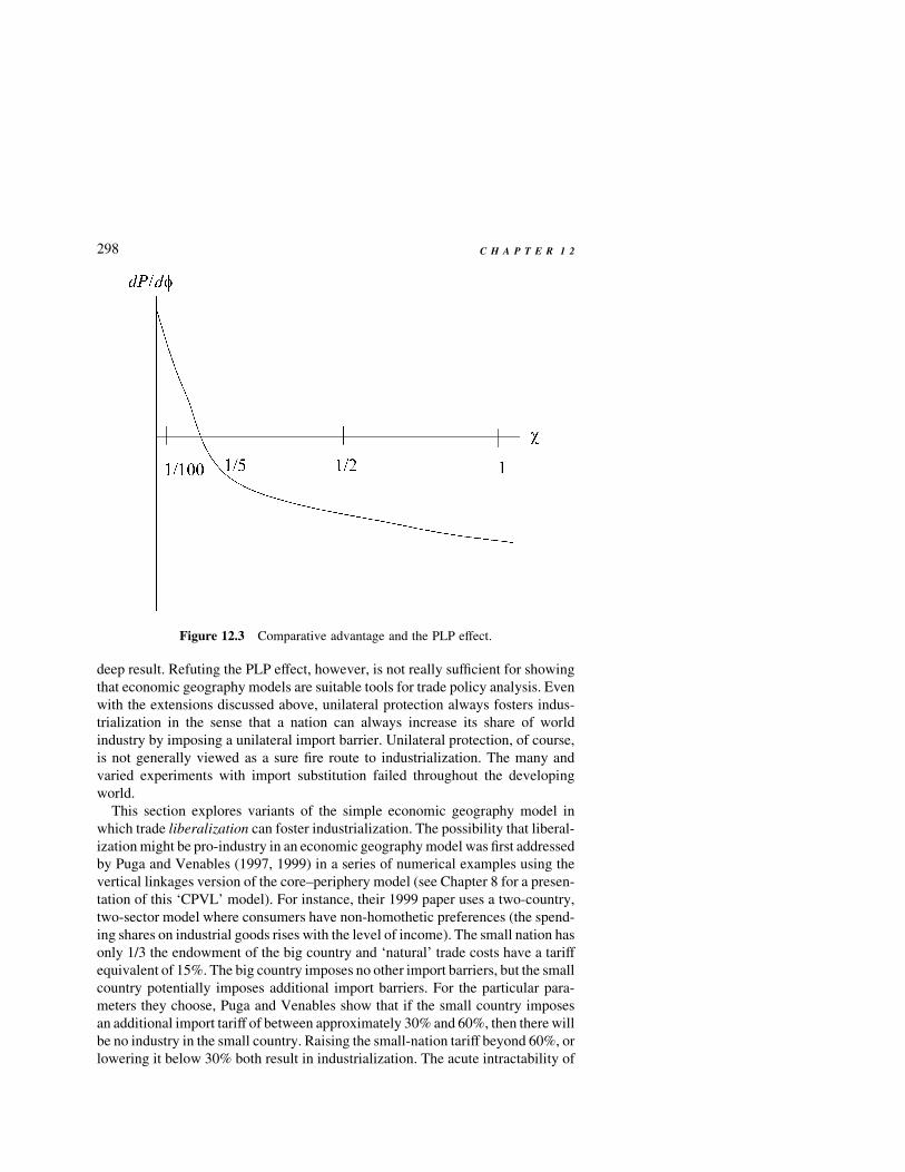
simulations. Figure 12.3 shows the results. The diagram has x on the horizontal

axis and the value of the derivative on the vertical axis. The simulation is done

assuming that the initial level of f is 0.5, and that m ¼ 4=10 and s ¼ 4. The

results confirm that the PLP effect holds only when comparative advantage is

weak. Numerically, the crossing point is between x ¼ 1=20 and x ¼ 1=100. When

we perform similar simulations for higher and lower values of the initial level of

trade freeness, we find qualitatively similar results. This line of exploration,

however, does reveal that for any level of x , the PLP effect is more likely to

hold when the initial level of trade freeness is high. This is expected since the

elasticity of delocation in this model increases dramatically with f .

12.3 Liberalization and Industrialization

The notion that unilateral protection always lowers the domestic price level by

enticing industry to relocate is certainly one of the most outlandish policy impli-

cations of simple economic geography models. The preceding section showed

that this was in fact an artefact of several simplifying assumptions rather than a

U N I L A T E R A L T R A D E P O L I C Y 297

deep result. Refuting the PLP effect, however, is not really sufficient for showing

that economic geography models are suitable tools for trade policy analysis. Even

with the extensions discussed above, unilateral protection always fosters indus-

trialization in the sense that a nation can always increase its share of world

industry by imposing a unilateral import barrier. Unilateral protection, of course,

is not generally viewed as a sure fire route to industrialization. The many and

varied experiments with import substitution failed throughout the developing

world.

This section explores variants of the simple economic geography model in

which trade liberalization can foster industrialization. The possibility that liberal-

ization might be pro-industry in an economic geography model was first addressed

by Puga and Venables (1997, 1999) in a series of numerical examples using the

vertical linkages version of the core–periphery model (see Chapter 8 for a presen-

tation of this ‘CPVL’ model). For instance, their 1999 paper uses a two-country,

two-sector model where consumers have non-homothetic preferences (the spend-

ing shares on industrial goods rises with the level of income). The small nation has

only 1/3 the endowment of the big country and ‘natural’ trade costs have a tariff

equivalent of 15%. The big country imposes no other import barriers, but the small

country potentially imposes additional import barriers. For the particular para-

meters they choose, Puga and Venables show that if the small country imposes

an additional import tariff of between approximately 30% and 60%, then there will

be no industry in the small country. Raising the small-nation tariff beyond 60%, or

lowering it below 30% both result in industrialization. The acute intractability of

298 C H A P T E R 1 2

Figure 12.3 Comparative advantage and the PLP effect.

the core–periphery model prevents them from pinning down a precise relationship

between their result and their particular assumptions (on the size asymmetry, the

level of natural trade costs, the extent of the non-homotheticity, the strength of

agglomeration forces, etc.). Their discussion, however, provides intuition that

suggests their findings are more general than the specific examples. This section

uses a variant of the vertical linkages variant of the footloose capital model to

analytically illustrate the Puga–Venables intuition.

12.3.1 Footloose Capital Model with Vertical Linkages

Studying the possibility of pro-industry liberalization, requires us to extend our

simple economic geography models to include intermediate goods, that is, ‘verti-

cal linkages’. The point is quite simple.

Without intermediates the only role of unilateral protection is to shift expen-

diture from foreign varieties to domestic varieties, so unilateral liberalization can

only reduce the attractiveness of the liberalizing nation to industry. If, however,

we make the natural and realistic assumption that industrial firms use imported

intermediates, liberalization takes on a new role. To the extent that liberalization

lowers the cost of imported intermediates, liberalization can lower the local cost

of production and thus—other things being equal—increase the attractiveness of

setting up an industrial firm in the liberalizing nation.

To make this point, we work with the ‘vertical linkages’ version of the

footloose capital model (or FCVL model for short). The model, due to Robert-

Nicoud (2002), is described at length in Chapter 8, so we just briefly review its

main features here. The basic set-up is identical to that of the FC model, namely

two sectors (M and A), two nations (home and foreign), and two factors (L which

is immobile and K which is perfectly mobile internationally). The supply assump-

tions for the Walrasian A sector are identical to those of the FC model, but quite

different for the M sector. Manufacturing firms use only capital as a fixed cost as

in the FC model while the variable costs compromise a Cobb–Douglas composite

of labour and intermediates. In particular, the intermediates are aggregated in the

standard CES composite, so the cost function for a typical variety is given by p 1

aMw12mPmm, where Pm is the standard CES price index.

Since capital moves freely in search of the highest reward, the location condi-

tion for an interior equilibrium is p ¼ p*. The local price indices are unimportant

since all capital earning is spent in the capital owner’s nation, regardless of where

the capital is employed. The condition for a core–periphery outcome is p . p*,

for the core-in-the north outcome and the opposite for the core-in-the-south

outcome. Importantly, in any of these equilibria, the reward to capital is always

the same regardless of the degree of openness and the spatial pattern of capital

employment.

The FCVL model displays both demand linkages (production shifting leads to

expenditure shifting since firms buy industrial goods as intermediates) and cost

linkages (since the CES price index falls as the local share of industry rises). As

such, it is not fully tractable in the sense that we cannot get a closed-form solution

U N I L A T E R A L T R A D E P O L I C Y 299

for the spatial allocation of firms, sn. Nevertheless, the model is significantly more

tractable than the vertical linkages version of the core–periphery model because

we can derive a function that gives the mobile factor’s reward in terms of the

spatial allocation of industry. See Chapter 8 for more on this comparison.

The location equilibrium can be described by three equilibrium expressions.

The expression for north and south rewards to capital is (with our normalizations

Ew ¼ 1, nw ¼ Kw ¼ 1)

p ¼ bsE

D1

fpspE

Dp

!Dm; pp ¼ b

fsE

D1

spE

Dp

!ðDpÞm ð12:30Þ

where f and f * are the north’s and south’s degree of trade freeness as usual and

the denominators of the demand functions, that is, the Ds, are implicitly defined

by

D ¼ nwðsnDm 1 fð1 2 snÞðD

pÞmÞ; Dp ¼ nwðfpsnDm 1 ð1 2 snÞðD

pÞmÞ ð12:31Þ

and the north’s relative market size is given by

sE ;Em

Ewm

¼ ð1 2 mÞsL 1 bsK 1m 2 b

bp sn ð12:32Þ

where Em stands for total expenditure on manufactures (this encompasses final

and intermediate demands). Before proceeding with the analysis, it is worth

noting several aspects of these expressions. First, the expression for p is very

similar to the one in the FC model, but it includes the extra term Dm, which

reflects the impact of the price of intermediates on a typical northern firm’s sales.

That is, if the CES price index, Pm ; D2m=ðs21Þ, is particularly high in the north,

then northern sales and, thus, p will be low. Second, the expressions for the Ds

cannot be solved analytically (except for special cases), so unlike the standard FC

model, the FCVL model is not fully tractable. Third, in the special case of

symmetric endowments (i.e. sL ¼ sK ¼ 1=2), an even division of industry

(sn ¼ 1=2) is always a solution, but it may not be stable. Moreover, as argued

in the Appendix 2.B, the break point comes before the sustain point, so the model

is subject to catastrophic agglomeration and locational hysteresis.

To explore the impact of liberalization, we first separate the role of protection

into its two components.

FINAL AND INTERMEDIATE GOODS: EFFECTIVE RATE OF PROTECTION

Protection affects industry through two distinct channels in a model with

imported intermediates—one channel functions via the local costs of imported

intermediates, the other by protecting local producers from import competition.

Intuition is served by separating these and to this end we suppose that the south-

ern government can, somehow, impose distinct import barriers on: (1) imports

that are sold to southern consumers; and (2) imports sold to firms as intermediate

inputs. For simplicity’s sake, we work with nations that are symmetric in terms of

endowments. Moreover, to focus on industrialization, we assume that the

300 C H A P T E R 1 2

common level of openness is just at the sustain point and all industry is agglom-

erated in the north. That is, writing the p ’s as implicit function of the north’s

share of industry, n, and the level of trade freeness, f , we have that

p½fS; n� ¼ p*½fS; 1 2 n�, where n ¼ 1. The axis of investigation is to determine

whether the southern government can, using an uneven liberalization, raise p *; if

it can, some industry will be attracted to the south since we start from the sustain

point. In other words, liberalization will foster industrialization.

The core–periphery outcome is one of the special cases where we can find the

Ds. With n ¼ 1, (12.31) implies that D ¼ 1 and D* ¼ f. Using these, and noting

that with n ¼ 1, northern demand depends on final and intermediate demand while

southern demand stems only from consumers, the expression for p * becomes

pp ¼1

s

fEm

11

Epm

fp

!ðfpgÞm; fp ¼ f ¼ fS ð12:33Þ

where f S is the sustain point level of openness and g . 1 reflects the extent to

which southern protection is higher on final goods than on imported intermediates.

Using Max Corden’s concept of the effective rate of protection, g . 1 implies that

the effective rate of protection on final goods is higher than f S.

Simple inspection of (12.33) reveals that increasing g—that is, liberalizing

imports of industrial goods for intermediate use—raises p *. Since p * was just

equal to p with n ¼ 1 in this example, we know that such a liberalization would

attract some industry to the south.

This type of trade liberalization can foster industrialization and indeed, most

developing nations do maintain higher levels of protection on final goods than

they do on intermediates. These practices lead to the creation of the notion of the

‘effective rate of protection’. That is, when intermediates and final goods are

protected at different rates, the true level of protection—the effective level—is

not well captured by the tariff rate on the final good.

EVEN PROTECTION

Is it possible that across-the-board liberalization could also foster industrializa-

tion? To check, we set g ¼ 1 and differentiate (12.33) with respect to f * to get

dpp

dfp ¼1

smfEm

12 ð1 2 mÞ

Epm

fp

!ðfpÞm21 ð12:34Þ

If this is positive, we know that unilateral liberalization can be beneficial to

industry. To characterize the sign of this expression, we solve for the f * that

makes it just zero. For any level off * above this critical value, liberalization will

be pro-industry. The critical value is ð1 2 mÞE*=ðmfEÞ. Since f * cannot exceed

unity, we see that liberalization can be pro-industrialization when the northern

market is relatively large and relatively open, and when the share of expenditure

on industrial goods is not too large. Intuition for these findings is simple. A small

size of the home market means that the part of the liberalization that affects

U N I L A T E R A L T R A D E P O L I C Y 301

import competition is small since home firms are mainly interested in the foreign

market to begin with. The openness of the foreign market plays the same role.

When the foreign market is very open, firms initially sell a large share of their

output to the foreign market, so the change in home openness has a dampened

impact on profits.

To summarize these results we write the following result.

Result 12.12 (pro-industrialization liberalization). Liberalization that

reduces the cost of imported intermediates without increasing import

competition in the market for final industrial goods tends to make the

liberalizing nation more attractive to industry. Moreover, even an

across-the-board liberalization can stimulate industry when the liberaliz-

ing nation is relatively small and the foreign market is relatively open.

12.4 Industrial Development, Market Size and Comparative Advantage

The previous section studied liberalization in a model where the cost of imported

intermediates affects the competitiveness of a nation’s industrial firms, showing

that, under some circumstances, unilateral opening could promote industrial

development. This section continues to focus on industrial development but

focuses on market size, comparative advantage and foreign trade barriers.

12.4.1 The Underdevelopment Puzzle

While rich country labour unions frequently bemoan the loss of ‘good’ manu-

facturing jobs to poor countries, most poor countries have the opposite complaint.

Given their low wages, why isn’t industry more interested in poor nations, that is,

why are poor countries so ‘underdeveloped’ in terms of industry?

The principal focus of economic geography models is industrial location, so

they provide a natural vehicle for studying the lack of industry in poor countries.

Before turning to the models, however, we address and then put aside the most

obvious answer.

Surely it is possible that poor countries have a comparative disadvantage in

manufacturing. Poor country wages are low because their workers are not very

productive. If this lack of productivity is either evenly spread across all sectors or

especially concentrated in manufacturing, then the unit cost of producing indus-

trial goods in developing nations will be higher than the unit cost in rich coun-

tries. The lower wages fail to offset the lower productivity, or—to use David

Ricardo’s terminology—poor nations have a comparative disadvantage in manu-

facturing. No wonder, then, that they have little industry. Even in a perfectly flat

world (no trade costs, no imperfect competition, no increasing returns), firms

would prefer manufacturing in rich countries.

While this classical explanation seems to account for the fact when it comes to

many poor nations, the rapid industrialization of several formerly poor nations

makes one wonder whether the full answer is not a bit more complex.

302 C H A P T E R 1 2

12.4.2 The ‘Peripherality Point’ in the FC and CC Models

The location of industry in a geography model depends upon relative market size

as well as the degree of domestic and foreign openness. Here, we add a third

concern, namely comparative advantage.

A convenient way to study the interaction of all these forces is to calculate what we

call the ‘peripherality point’, that is, the smallest market size that permits the small/

poor nation to attract at least some industry. Following the principle of progressive

complexity, we start with the easiest model, the FC model of Chapter 3.

To be concrete, we consider the north to be the small (poor) nation that is

struggling to promote industrial development when all industry is initially located

in the large (rich) south. To add an important real-world element to the equation,

we modify the standard FC model to allow for technology differences.

Ricardian comparative advantage can be easily introduced into the FC model

by assuming that the ratio of labour input coefficients differs in the two nations. In

particular, we assume that the north’s ratio aM/aA differs from the south’s a*M=a

*A,

where the ai’s are sectoral unit labour requirements using our standard notation.

To introduce this enrichment with the least complication, we assume that, as in

the basic FC model, aA ¼ a*A ¼ 1, so free trade in A goods continues to equalize

nominal wages in both nations (i.e. we assume that the no-full-specialization

condition holds; see Chapter 3 for details). With this modification, the rewards

to capital are

p ¼ bsE

D1

fpð1 2 sEÞ

Dp

!x; pp ¼ b

fsE

D1

1 2 sE

Dp

� �; x ;

aM

apM

!12s

ð12:35Þ

where

D ¼ xsn 1 fð1 2 snÞ; Dp ¼ fpxsn 1 1 2 sn

and x (a mnemonic for comparative advantage) measures comparative advantage

with x . 1 indicating a comparative advantage for the north in industry; note that

the x here is entirely unrelated to the x in (12.25). Recall that in the FC model,

the north’s relative market size, as measured by sE, is exogenous.

Solving the location condition p ¼ p* for the spatial division of industry, sn,

allowing for differences in size, openness and comparative advantage, we have

sn ¼½ð1 2 sEÞff

p 1 sE�x 2 f

ðx 2 fÞð1 2 xfpÞð12:36Þ

where, as usual, this is only valid for economically relevant shares; if the right-

hand side exceeds unity or is less than zero, then sn is one or zero as appropriate.

As usual, real incomes depend upon industrial location and openness. If both

countries are equally open, then, as usual, the small country will have less

industry and, thus, a higher price index. In other words, the small country will

also be the poor country.

U N I L A T E R A L T R A D E P O L I C Y 303

Although our expressions are general, we are particularly interested in the case

where x . 1, that is, where the small/poor/un-industrialized nation actually has a

fundamental comparative advantage in industry. The interest lies in the fact that,

in a neoclassical model, the small north would always have some industry regard-

less of trade costs. In an economic geography model, by contrast, market-access

considerations can allow a pattern of specialization that contradicts comparative

advantage. Furthermore, since wages are equalized, yet the north has a lower

labour input coefficient in industry, the unit cost of industrial production is lower

in the north.

To find the peripherality point, we find the sE where sn is just equal to zero, that

is, where the core-in-the-south is just barely sustained. Solving sn¼ 0, where sn is

(12.36), for sE, we get the critical market size of the rich/northern market to be

sPE ¼

f

1 2 ffp

1

x2 fp

� �ð12:37Þ

where sEP is the peripherality point, that is, the size of the small northern market

that implies it has no industry. Since (12.36) is increasing in sE, we know that the

north will be without industry (i.e. will be the periphery) for any market size that

is less than sEP.

A particularly salient feature of (12.37) is that, even if the north has a native

comparative advantage in industry (x . 1) so that the unit labour cost of produ-

cing in the north is below that of the big south, industry can still be fully concen-

trated in the south. In other words, this is an example of agglomeration producing

a trade pattern that contradicts the pattern predicted by comparative advantage.

DISCUSSION

Expression (12.37) conveniently organizes the various forces that foster industrial

underdevelopment. By inspection, sEP is decreasing in x and inf *, and increasing in

f . This means that the greater is the north’s comparative advantage in manufactur-

ing, the smaller its market must be to sustain peripherality. Moreover, protection of

the big market (the south in this case) makes location in the small north less advan-

tageous, so higher big-market protection (df* , 0) allows northern peripherality at

a higher northern market size. The impact of small-nation protection on the small

country was thoroughly explored in the previous section so there is no need to repeat

it here. To summarize, we write the following results.

Result 12.13 (size matters). If agglomeration forces are important and

trade is not completely costless, small nations will tend to be without

industry. The minimum market size that is necessary to attract some indus-

try depends upon openness and comparative advantage (these are the

subject of subsequent results).

Result 12.14 (GSP logic). The higher are industrialized nations’ barriers

against the industrial exports of the poor countries, the more likely it is that

small nations will be without industry and thus poor.

304 C H A P T E R 1 2

This may be thought of as providing some intuition for why the WTO’s General-

ised System of Preferences (GSP) was thought to be pro-development.12

The final result concerns the small nation’s trade barriers. The more open the

small nation is to big-nation industrial exports, the larger must be the small

nation’s market to attract at least some industry. Of course, we have seen in

the two previous sections that this import-substitution logic can be reversed

when one allows for other real-world elements such as capital relocation costs

and intermediates.

12.4.3 Allowing for Self-Reinforcing Agglomeration

While the FC model is supremely amenable to analysis, it achieves this by

assuming away many interesting aspects of more general economic geography

models. We can restore one major element—circular causality, that is, self-rein-

forcing agglomeration—by re-doing the analysis in the CC model of Chapter 6.

That model allows for demand-linked circular causality by assuming that capital

is constructed (rather than endowed) and that it must be employed in its region of

origin. Forces that encourage industry in a particular nation result in an incentive

to raise that nation’s capital stock. Because national expenditure also rises with

the capital stock, we have that forces that tend to ‘shift’ production to a nation

also tend to ‘shift’ expenditure to that same nation. Since this cycle of production

and expenditure strengthens agglomeration forces, it also exaggerates the spatial

implications of any given policy change.

The main difference that appears when we shift from the FC model to the CC

model is that the spatial division of expenditure, that is, the relative market

sizes—as measured by sE—becomes endogenous. In particular, the expressions

(12.35) and (12.36) are equally valid for the CC model, but additionally we have

sE ¼ ð1 2 bÞsL 1 bsn; 0 , b ;br

r 1 d, 1 ð12:38Þ

where b ; m=s as usual, r is the discount rate and d . 0 is the rate of deprecia-

tion (see Chapter 6 for details). Solving the location condition, p ¼ p*, using

(12.35) and (12.38), we get a formula for sn and solving this for the sL where sn¼

0, we find the CC-model’s peripherality point to be

sPL ¼

f

1 2 ffp

1

x2 fp

� �1

1 2 bð12:39Þ

To compare this to the equivalent expression for the FC model, suppose that north

and south have identical relative endowments (i.e. sL ¼ sK), so that sE ¼ sL. In

this case, we can directly compare (12.39) and (12.37). Because 0 , b , 1, the

point of peripherality is higher in the CC model. This is quite intuitive. It says that

the small nations need a bigger market to attract at least some industry when

agglomeration forces are stronger. Indeed, b is a measure of the strength of

U N I L A T E R A L T R A D E P O L I C Y

12 GSP is a GATT waiver of the non-discrimination principle. It allows rich nations to provide

preferential market access to the industrial exports of poor nations.

305

agglomeration forces in the CC model (e.g. the break point is ð1 2 bÞ=ð1 1 bÞ

with symmetric nations), so we get the very believable result that the stronger are

agglomeration forces, the larger a nation must be before it can support some

industry. To summarize, we write the following result.

Result 12.15 (agglomeration forces and the peripherality point). The

peripherality point calculated for the FC model is higher than that for the

CC model since agglomeration forces are stronger in the CC model. More-

over, the stronger are agglomeration forces in the CC model, the larger a

nation must be before it can support some industry.

12.5 Location and Policy Non-Equivalences

When firms operate in a competitive environment, tariffs and quotas are ‘equiva-

lent’ under a broad range of assumptions. That is, a tariff and a quota that restrict

imports to the same extent, have the same impact on prices—be they consumer

prices, producer prices or import prices. The distribution of trade rents (i.e.

imports times the gap between domestic and border prices) between foreign

and domestic residents may differ depending upon how the quota is administered,

but if the government auctions the quota licences, then tariffs and quotas are

equivalent in this aspect as well.

This section explores the implications of economic geography for the classical

tariff–quota equivalence. Before turning to the geography models, we illustrate

the basic equivalence insight with a partial equilibrium to fix ideas and introduce

notation. Consider first a specific tariff equal to the difference between the domes-

tic and border prices shown as pb and pd in Figure 12.4. This drives a wedge

between the import demand curve (MD) and the import supply curve (MS), so

compared to the free trade outcome, the tariff reduces imports from M to M 0. The

gain in trade rents (i.e. tariff revenue), which equals A 1 B, tends to offset the loss

in private surplus, namely 2A 2 C. Indeed, the tariff enables home to tax

foreigners (B is the incidence of the tax on foreigners) and if the incidence on

foreigners exceeds the part of the deadweight loss that falls on domestic resi-

dents, that is, C, the tariff raises domestic welfare as measured by the unweighted

sum of private and public surpluses.

A quota that restricted imports to M 0 would have identical effects on prices and

quantities. If quota rights are allocated to home residents, the trade rents continue

to count towards the home surplus and the total welfare impact is identical to that

of the tariff. If the quota rights are allocated to foreigners, the trade rents no

longer count in the sum of domestic surpluses and the result is a sure loss for

home of 2A 2 C. It is worth noting that since pd is the price home pays for its

imports when foreigners have the quota rights, the impact on home welfare is

identical to the terms of trade loss that would result from a rise in the border price

from the free-trade price to pd.

This reasoning suggests that it is useful to categorize trade barriers according

to their trade rent allocation implications. Trade barriers, such as tariffs and

306 C H A P T E R 1 2

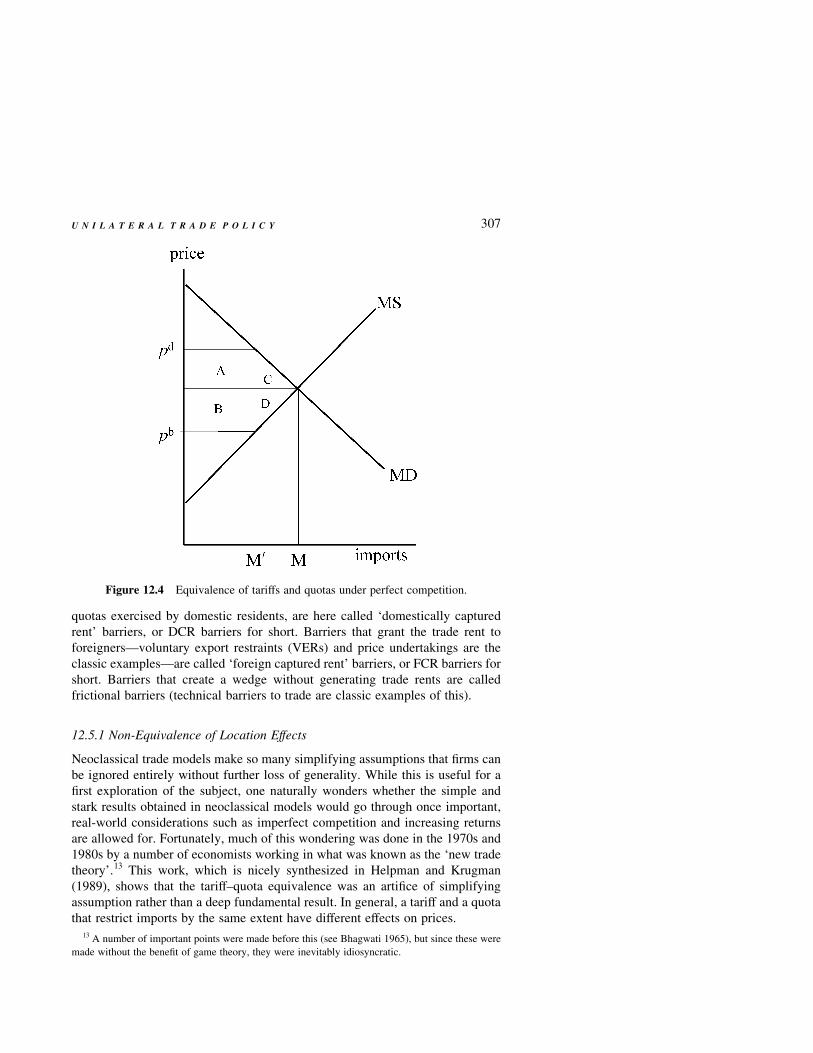
quotas exercised by domestic residents, are here called ‘domestically captured

rent’ barriers, or DCR barriers for short. Barriers that grant the trade rent to

foreigners—voluntary export restraints (VERs) and price undertakings are the

classic examples—are called ‘foreign captured rent’ barriers, or FCR barriers for

short. Barriers that create a wedge without generating trade rents are called

frictional barriers (technical barriers to trade are classic examples of this).

12.5.1 Non-Equivalence of Location Effects

Neoclassical trade models make so many simplifying assumptions that firms can

be ignored entirely without further loss of generality. While this is useful for a

first exploration of the subject, one naturally wonders whether the simple and

stark results obtained in neoclassical models would go through once important,

real-world considerations such as imperfect competition and increasing returns

are allowed for. Fortunately, much of this wondering was done in the 1970s and

1980s by a number of economists working in what was known as the ‘new trade

theory’.13 This work, which is nicely synthesized in Helpman and Krugman

(1989), shows that the tariff–quota equivalence was an artifice of simplifying

assumption rather than a deep fundamental result. In general, a tariff and a quota

that restrict imports by the same extent have different effects on prices.

U N I L A T E R A L T R A D E P O L I C Y

Figure 12.4 Equivalence of tariffs and quotas under perfect competition.

13 A number of important points were made before this (see Bhagwati 1965), but since these were

made without the benefit of game theory, they were inevitably idiosyncratic.

307

The basic reasons why tariffs and quotas are not equivalent under imperfect

competition and increasing returns are well understood. However, the differential

impact that such policies have on the spatial allocation of industry has not been

explored. This section is a first attempt to highlight the main issues and provide

insight on the non-equivalent location effects of tariffs and quotas. Following the

principle of progressive complication, we start with a very simple example to

provide intuition, before moving on to a more standard framework (Dixit–Stiglitz

monopolistic competition).

12.5.2 Tariff vs. Quota: The Case of the ‘Lonely’ Monopolist

We start with a simple example, namely, the case of a monopolist and this is most

easily embedded in the linear FC model of Chapter 5. The model is developed at

length there, but we present the basic elements here for the reader’s convenience.

The supply side of the economy is identical to that of the FC model employed above,

so again there are two sectors, two nations and two factors. Costless trade in the

Walrasian sector and costless capital mobility equalize factor prices internationally.

Each variety of industrial good entails a fixed cost of one unit of capital, so the spatial

distribution of capital and industry are identical. The main difference comes on the

demand side. Preferences are assumed to be quasi-linear with the Walrasian good

acting as the ‘outside’ good and tastes for industrial varieties given by a quadratic

sub-function. The preferences yield linear demand curves for each industrial variety;

spending on the Walrasian good is a residual.

To deal with monopoly power as simply as possible in this section, we assume

away substitutability among different industrial varieties in consumer tastes, so

that each producer can be thought of as a ‘lonely’ monopolist. Finally, we assume

that the monopolist we focus on is currently located in the south and transporta-

tion costs are low enough so that he/she serves both markets.

Demands by northern and southern consumers are Lða 2 bpÞ and L*ða 2 bp*Þ,

respectively, where p and p* are consumer prices, L and L* are market sizes, and a

and b are positive parameters (the a and b in this section are completely unrelated

to the a and b used above). For simplicity, we normalize marginal production

costs to zero. Inter-regional transportation costs are t, and trade is further

restricted by a specific tariff equal to l (recall that transportation costs involve

the numeraire good in the linear model so they are not iceberg costs). Tariffs are

collected in the numeraire good and returned lump sum to domestic residents, so

tariff revenue has no effect on demand. Finally, we assume that markets are

segmented in the sense that firms can price discriminate between the two markets

without worrying about arbitrage.

With these assumptions, the monopolist chooses prices to maximize operating

profits, which are

pp ¼ Lða 2 bpÞðp 2 t 2 lÞ1 Lpða 2 bppÞpp ð12:40Þ

since the monopolist is in the south. As usual, optimal pricing with linear demand

implies p* ¼ a=2b and p ¼ p* 1 ðl 1 tÞ=2. Since the monopolist must hand over

308 C H A P T E R 1 2

l units to the northern government for every unit sold in the north, equilibrium

profits are

pp ¼ bðL 1 LpÞðppÞ2 2 bLðl 1 tÞpp 1 bLl 1 t

2

� �2

; pp ¼a

2bð12:41Þ

Clearly, profits decrease with both the transportation cost, t, and the trade barrier,

l, over the parameter space for which we get interior solutions for prices and

quantities (so that some trade occurs at equilibrium).

WHO GETS THE TRADE RENTS?

We have started by supposing that l is a tariff, so the northern government

collects tariff revenues (i.e. trade rents) worth

R ¼ lLb pp 2t 1 l

2

� �ð12:42Þ

If the trade barrier takes the form of a quota, the monopolist, who can perfectly

price discriminate across markets, will charge a price to northern consumers that

is just high enough to ensure that they only want to consume (i.e. import) an

amount equal to the quota. Supposing that the quota is set to restrict imports to

exactly the same level that would have been observed under a tariff equal to l ,

the monopolists will continue charging the same consumer prices that he/she did

under the tariff, and this means that the trade rents, (12.42), accrue to the southern

monopolist rather than the northern government.

The formal argument behind this result can be found in Helpman and Krugman

(1989), but the intuition is easy. If the monopolist charges a northern consumer

price below p* 1 ðl 1 tÞ=2, demand will exceed the quota, so some other agent

will have to absorb the rents created by the quantity rationing. This plainly is not

profit-maximizing behaviour for the monopolists. If the monopolist found it

optimal to charge a price above p* 1 ðl 1 tÞ=2, northern demand will be less

than the quota and the quota is not binding. But if the quota is not binding, the

monopolist would ascribe a shadow price of zero to the restriction and thus his/

her optimal price in the northern market would be p* 1 t=2 and this would result

in a level of imports that exceeded the quota. What this shows is that the hypoth-

esis that the monopolist might find it optimal to charge a price above p* 1 ðl 1

tÞ=2 leads to a logical contradiction and so must itself be false. Finally, we note

that both tariff and quota reduce profits vis-a-vis free trade (i.e. l ¼ 0) since they

impose constraints on the monopolist’s otherwise unconstrained problem. In

summary, we have the following result.

Result 12.16. A tariff and a quota that result in the same level of imports

both reduce the profit earned by a foreign monopolist, but the quota is less

harmful to profits since the home government gets the trade rents with the

tariff, while monopolist gets them with a quota. The two policy instruments

have the same impact on consumer prices.

U N I L A T E R A L T R A D E P O L I C Y 309

IMPLICATIONS FOR LOCATION

With this simple framework in mind, we now make two simple points related to

the non-equivalence of the location effects of tariffs and quotas.

First, we note that even in this framework, protection may lower domestic

prices. Starting with symmetric nations and free trade, any northern tariff or

quota—however small—will induce the monopolist to relocate to the protected

market. To see this in the case of a tariff, write p as the profit of the producer

when located in the north. Since the expression for the equilibrium, p , is

isomorphic to (12.41) with l ¼ 0, the gain from relocating to the north is

p 2 pp ¼lL

2a 2 b

l 1 2t

2

� �ð12:43Þ

which is positive by virtue of the usual parameter restriction. In addition, because

p . p*, this relocation would lower the price faced by northern consumers (they

would no longer pay the share of transportation costs that was previously passed onto

them). The result is that any positive trade barrier, l, would produce the PLP effect.

Second, the nature of the trade barrier matters for the location equilibrium and,

in turn, for the cost-of-living (the consumer price index). To see this, assume now

that the two regions are of different sizes. In particular, we take north to be the

small market (L , L*). Now, starting from a situation where the monopolist is in

the south, suppose the north imposes a tariff. A relocation to the north would yield

a net gain of

p 2 pp ¼lL

2a 2 b

l 1 2t

2

� �2

tðLp 2 LÞ

2a 2 b

t

2

� �ð12:44Þ

which reduces to (12.43) when L ¼ L*. The terms in both large parentheses above

are positive. The first term on the right-hand side represents, as before, the profits

saved on tariffs by relocating to the protectionist country. The second term

represents the loss of profits involved by relocating away from the large country;

obviously, this loss is nil when transportation costs, t, are zero. Since the two

terms pull profits in opposite directions, the net impact of l on the relocation

decision is ambiguous. To illustrate the non-equivalence of tariffs and quota on

location, assume that l and L/L* combine such that the profit change in (12.44) is

just positive, namely

l

ta 2 b

l 1 2t

4

� �¼

Lp 2 L

La 2 b

t

2

� �1 1 ð12:45Þ

where 1 is an arbitrarily small positive number, so the monopolist would delocate

to the north.

We now ask: What happens if home is forced to replace its tariff with an

equivalent quota? Since a quota is less harmful to a south-based monopolist

than a tariff, the gain from delocating to the north would be lower. Since the

monopolist was almost indifferent to relocation with the tariff, he/she would be

against relocation if the protection took the form of a quota. Specifically, using

(12.42), the prospective gain (12.44) is now replaced by

310 C H A P T E R 1 2

p 2 pp ¼ L1t

22 l

a 2 bðl 1 tÞ

2

� �ð12:46Þ

which is negative for 1 and t small enough. Hence, when regions are of different

sizes, the small region might fail to attract the foreign producer.

The key implication of this is that a tariff would result in lower domestic prices,

while a quota would result in higher domestic prices. Moreover, although the

tariff and the quota would have the same impact on imports without delocation,

the tariff ends up reducing imports to zero, while the quota restricts imports less

drastically. This is summarized in the following result.

Result 12.17. A tariff and a quota calculated to result in the same level of

imports based on initial production patterns can have radically different

effects once relocation possibilities are allowed for. In particular, if the

tariff is just large enough to induce the foreign monopolist to delocate to

the north, the ‘equivalent’ quota will fail to induce delocation. As a conse-

quence, the tariff would result in a drop in domestic prices and a cessation

of imports, while the quota would raise domestic prices and only partially

restrict imports. This suggests that policies that favour tariffs over quotas

have an impact on location in themselves.

The point that relative market size matters for the PLP effect was made in the

previous section. The additional insight here is that the nature of the protection

also matters.

Having made these simple points in a simplistic model, we turn to verifying the

main insights in a richer economic environment. In particular, our example was

also extreme in the sense that the monopolist had no interaction with any other

producer. We turn to showing that these points generally hold in the other

extreme case, namely, in the FC model.

12.5.3 Tariff vs. Quota in the FC Model

In the FC model, each producer has a monopoly in the product for his/her specific

variety, competing with other firms only indirectly. Having shown above that a

monopolist earns higher operating profit in a market that is protected with a quota

than in a market that is protected with a tariff, we know that quotas will typically

affect the reward to capital. Because operating profit is part of expenditure, this

sort of effect will alter the two region’s relative expenditures and thus remove a

great deal of the FC model’s tractability. Since this sort of connection between

market size and the nature of protectionist barriers is surely of second-order

importance in the real world, we neutralize the connection by working with

quasi-linear preferences (see Appendix 2.A for details). The main implication

is that the demand functions for industrial goods no longer depend upon region

incomes. In particular, the demand functions are

cp ¼ðm=2Þpp2s

np12s 1 nppp12s; c ¼

ðm=2Þp2s

np12s 1 nppp12sð12:47Þ

U N I L A T E R A L T R A D E P O L I C Y 311

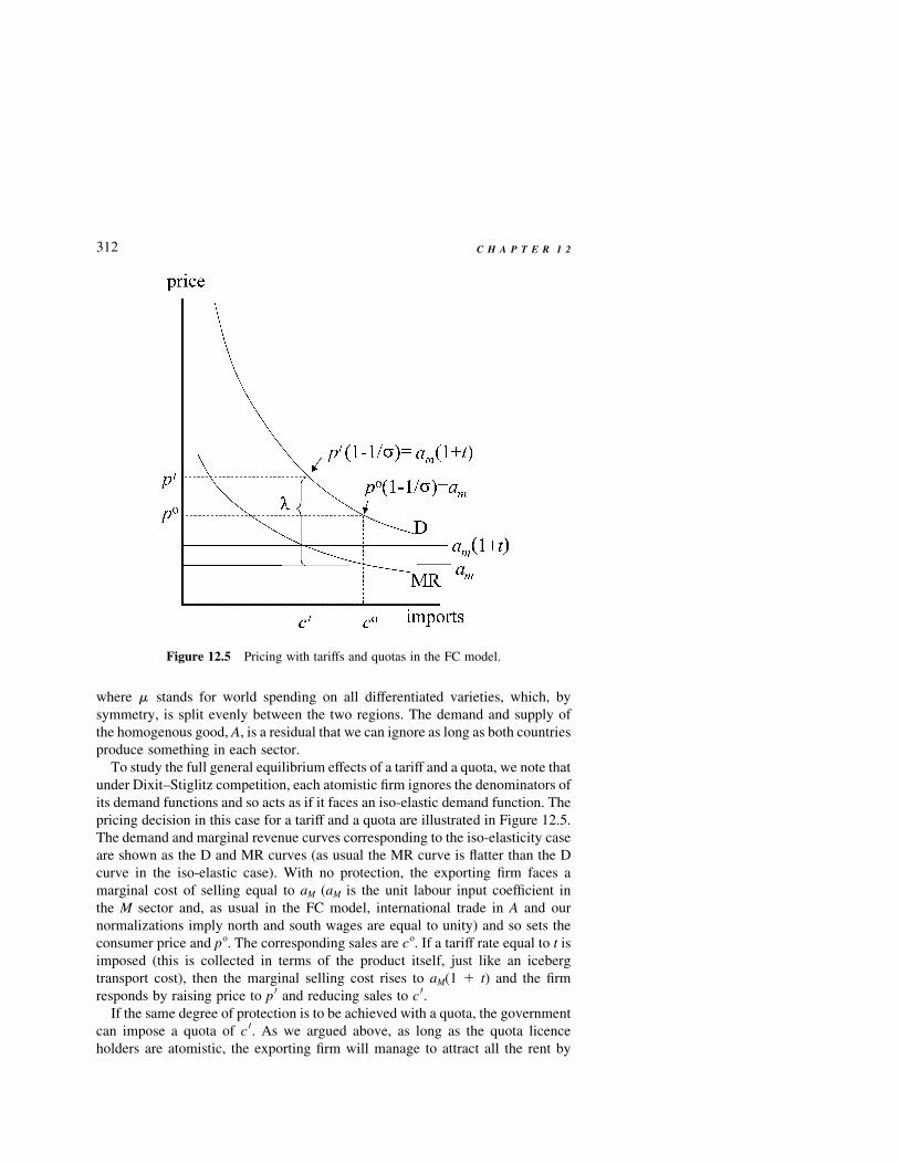
where m stands for world spending on all differentiated varieties, which, by

symmetry, is split evenly between the two regions. The demand and supply of

the homogenous good, A, is a residual that we can ignore as long as both countries

produce something in each sector.

To study the full general equilibrium effects of a tariff and a quota, we note that

under Dixit–Stiglitz competition, each atomistic firm ignores the denominators of

its demand functions and so acts as if it faces an iso-elastic demand function. The

pricing decision in this case for a tariff and a quota are illustrated in Figure 12.5.

The demand and marginal revenue curves corresponding to the iso-elasticity case

are shown as the D and MR curves (as usual the MR curve is flatter than the D

curve in the iso-elastic case). With no protection, the exporting firm faces a

marginal cost of selling equal to aM (aM is the unit labour input coefficient in

the M sector and, as usual in the FC model, international trade in A and our

normalizations imply north and south wages are equal to unity) and so sets the

consumer price and po. The corresponding sales are co. If a tariff rate equal to t is

imposed (this is collected in terms of the product itself, just like an iceberg

transport cost), then the marginal selling cost rises to aM(1 1 t) and the firm

responds by raising price to p 0 and reducing sales to c 0.

If the same degree of protection is to be achieved with a quota, the government

can impose a quota of c 0. As we argued above, as long as the quota licence

holders are atomistic, the exporting firm will manage to attract all the rent by

312 C H A P T E R 1 2

Figure 12.5 Pricing with tariffs and quotas in the FC model.

setting a price equal to p 0. In other words, the Lagrangian multiplier on the quota

constraint must be equal to the l shown in the diagram. Plainly, the operating

profit margin is higher with a quota than with the ‘equivalent’ tariff and, as a

result, southern operating profit earned on northern sales is higher under a quota.

Specifically, it is higher by the rectangle ð1 1 tÞc 0.

THE SPATIAL EQUILIBRIUM

We now turn to a more formal treatment of the problem. As a matter of conven-

tion, we take the north as the protecting economy and consider the effects of the

trade policies on south-based producers of industrial varieties.

As usual, the fulcrum for our investigation is operating profits of south-based

and north-based firms. As before, t represents either the iceberg transportation

cost or an ad valorem tariff, and l reflects the shadow price of any quota. Here,

however, it proves insightful to allow for both natural transport costs, what we

call ‘T’’ and a tariff, denoted as ‘t’. Thus, t ; 1 1 T 1 t, where T is an exogen-

ously given parameter while t is chosen by the northern government. The

problem of a typical south-based firm is

maxp;pp ðpSS 2 aMÞxSS 1 ðpSN 2 aMtÞxSN s:t: xSN # Q ð12:48Þ

Here, we adopt a more explicit notation where, for example, pij is the price

charged by a firm located in market i for sales in market j; the x’s indicate

sales using the same notation.

The solution to this maximization problem provides optimal prices and a

shadow value on the quota. Employing our usual normalization of

b ¼ 1 2 ð1=sÞ, these are

pSN ¼ t 1 l=aM ; pSS ¼ 1 ð12:49Þ

Using these in (12.48), and using the standard FC model solution for northern

operating profits (only the north imposes barriers in our example), we have

p ¼ bð1

D1

fp

Dp Þ; pp ¼ bfz

D1

1

Dp

� �

f ; t 1l

aM

� �12s

; z ;t 1 ls=aM

t 1 l=aM

� �$ 1 ð12:50Þ

where the northern trade freeness, f , allows for tariff or quota protection, and the

Ds are defined as in (12.5).14 The z term, which exceeds unity when the quota is

binding, reflects the fact that south-based firms earn an extra high operating profit

margin on sales to a market protected with a quota.

U N I L A T E R A L T R A D E P O L I C Y

14 Having assumed a segmented market, we can explain the term with z by dealing only with the

sub-problem of a typical southern firm’s sales to the north: maxpðp 2 btÞx, s.t. Q $ x. The first-order

condition is pð1 2 ð1=sÞÞ ¼ bt 1 l, where l is the Lagrangian multiplier on the quota. Rearranging

this, we have ðp 2 btÞx ¼ px=s 1 lx. As long as the quota is binding, l . 0 and the operating profit

earned on sales to the north exceeds the usual amount, that is, px=s. Using z ; 1 1 sl=p and the first-

order condition, with b ; ð1 2 ð1=sÞÞ, yields the result.

313

Capital searches for the location with the highest reward so the interior equili-

brium is where p ¼ p*. Solving this location condition for the spatial equili-

brium, sn, gives

sn ¼1

21

fp 2 f 1 fpð1 1 fÞ2 ð1 1 fpÞfz

2ð1 2 fpÞ½2 2 ð1 1 zÞf�ð12:51Þ

so when the north imposes no protection (l ¼ t ¼ 0, so f ¼ f* ¼ ð1 1 TÞ12s),

this says that industry is evenly split, that is, sn ¼ 1=2.

EQUALLY PROTECTIONIST TARIFFS AND QUOTA

tariff and a quotaThe difference between tariff and quota protection can be illu-

strated with the following experiment. Suppose in the first case that the north

unilaterally protects its market with a tariff only (t . l ¼ 0), and the south does

not respond. The northern market will be less open than the southern market and,

to be specific, we define the difference as d ; f*=f $ 1. In the second case, the

north imposes the same degree of protection—in the sense that d ; f*=f—but

now it uses only a quota (l . t ¼ 0). Both instruments will alter the locational

equilibrium; specifically,

sn ¼f2d 1 1 2 ð1 1 zÞf

ð1 2 dfÞð2 2 ð1 1 zÞfÞð12:52Þ

When the protectionist instrument is a tariff,z ¼ 1, and when it is a quota, z . 1.

By inspection, we can see that the delocation effect of the tariff is greater than that

of the quota. The intuition for this is straightforward. The fact that the quota tends

to boost the profitability of southern exports to the north means that the quota

tends to keep more of the southern firms in place.

Given this, we can use the reasoning of the previous section to say that a tariff

will have a more negative impact on north’s price than will a quota.

There is another more important difference between the tariff and quota protec-

tion. In the case of a tariff, the delocation flow continues until the reward to north-

based capital returns to the level it was at before the protection. Specifically, it

equals b before and after the tariff protection. With a quota, however, both the

northern and southern rewards to capital are higher with the quota than without.

Intuitively, the reason is that the quota raises the operating profit margin on one

trade flow (southern exports to the north) and this raises the total level of operat-

ing profit worldwide. While relocation ensures equalization of p , the equaliza-

tion takes place at a higher level. It has often been remarked that firms typically

prefer quota protection to tariff protection. Our analysis suggests one possible

explanation. If the north-based firms manage to overcome the free-rider problem

and organize to lobby for a tariff, the potential rise in their earnings that a tariff

tends to create will be entirely eroded by foreign entry. By contrast, lobbying for

a quota will allow them to raise their reward and so may justify the lobbying

expense. Note also, that the foreign producers will similarly prefer a quota to a

tariff.

314 C H A P T E R 1 2

More formally, using (12.52) in (12.50), the sum of world operating profit,

namely nw½snp 1 ð1 2 snÞp�, is

b1 2 df2z

ð1 2 df2Þ

!1 2 fð1 1 zÞ=2

1 2 zf

� �ð12:53Þ

where we have used the standard normalization of nw ¼ 1. Since each term in the

large parentheses is greater than unity when z . 1, we see that world profits are

higher under a tariff than under a quota. This is summarized in the following result.

Result 12.18. A quota and tariff that produce the same level of imports have

different effects on the geographical dispersion of industry, on domestic

prices and on the reward to capital. In particular, since a quota is better for

foreign exporters than a tariff, the quota produces less delocation into the

protected economy (i.e. the tariff-jumping delocation will be greater than

the quota-jumping delocation). The reduced delocation also means a quota

has a dampened PLP effect. Furthermore, the quota will raise the equili-

brium reward to capital in both regions, while the tariff’s profit boosting

effect is entirely offset by delocation.

Of course, if the level of protection is high enough to induce total delocation to

the protected economy, then a trivial equivalence is restored.

POLITICAL ECONOMY CONSIDERATION AND FURTHER CONSIDERATIONS

We have examined tariffs and quotas in a setting where the PLP effect always

works; above we saw that this was really just an artefact of the model’s simplify-

ing assumptions. In richer frameworks, the price-index-lowering effect of protec-

tion-induced delocation may or may not offset the direct price-index-raising

effect of protection. It is clear that we could easily build an example in which

a tariff would reduce domestic prices whilst a quota would increase them.

We have left aside an important, potentially interesting, issue here. In both our

examples, market conduct is either trivial (the lonely monopolist) or simplistic

(monopolistic competition). In either case, each producer does not interact

directly with others. It would be interesting to know how the market conduct

could be affected by the nature of the policy instrument. For instance, can we

imagine a situation where a quota so strongly boosts the profits of foreign expor-

ters that the quota leads to delocation out of the protected economy? More

generally, how do the location effects of VERs and quotas differ in settings of

imperfect competition? Our preliminary explorations suggest that these issues are

harder to answer than one might think; we leave them for future research.

12.6 Concluding Remarks

This chapter just scratches the surface of what seems to be a field rich in inter-

esting results. For instance, we have looked only superficially at the underdeve-

U N I L A T E R A L T R A D E P O L I C Y 315

loped puzzle. The numerical examples in Puga and Venables (1998) suggest that

many more interesting results could be demonstrated in the more tractable

models in Part I. Another example of ‘low hanging fruit’ concerns path depen-

dencies. The chapter does not follow up on one of the most usual aspect of

geography models, namely locational hysteresis. It would be of some interest,

for instance, to consider how temporary unilateral protection could permanently

alter trade patterns, perhaps creating ‘un-natural’ comparative advantages.

References

Baldwin, Richard E. and F. Robert-Nicoud. 2002. Asymmetric lobbying: why govern-

ments pick losers. Working Paper No. 8756, National Bureau of Economic Research.

Bhagwati, J. 1965. On the equivalence of tariffs and quotas. In Trade, Growth and the

Balance of Payments, ed. R. E. Caves, H. G. Johnson and P. B. Kenen. Amsterdam:

North-Holland.

Forslid, R. and I. Wooton. 2001. Comparative advantage and the location of production.

Review of International Economics in press.

Helpman, Elhanan and P. Krugman. 1989. Trade Policy and Market Structure. Cambridge,

MA: MIT Press.

Puga, Diego and A. Venables. 1997. Preferential trading arrangements and industrial

location. Journal of International Economics 43(3–4): 347–368.

______. 1999. Agglomeration and economic development: import substitution vs trade

liberalisation. Economic Journal 109(455): 292–311.

Robert-Nicoud, F. 2002. A simple model of agglomeration with vertical linkages and

capital mobility. Mimeo, London School of Economics.

316 C H A P T E R 1 2