Embed Size (px)
Citation preview
Unifying QuantumElectrodynamics and
Many-Body Perturbation TheoryIngvar Lindgren
Department of Physics
University of Gothenburg, Gothenburg, Sweden
Slides with Prosper/LATEX – p. 1/48
New Horizons in Physics
Makutsi, South Africa, 22-28 November, 2015
In honor of Prof. Walter Greinerat his 80
th birthday
Slides with Prosper/LATEX – p. 2/48

CoworkersSten SalomonsonDaniel HedendahlJohan Holmberg
Slides with Prosper/LATEX – p. 3/48
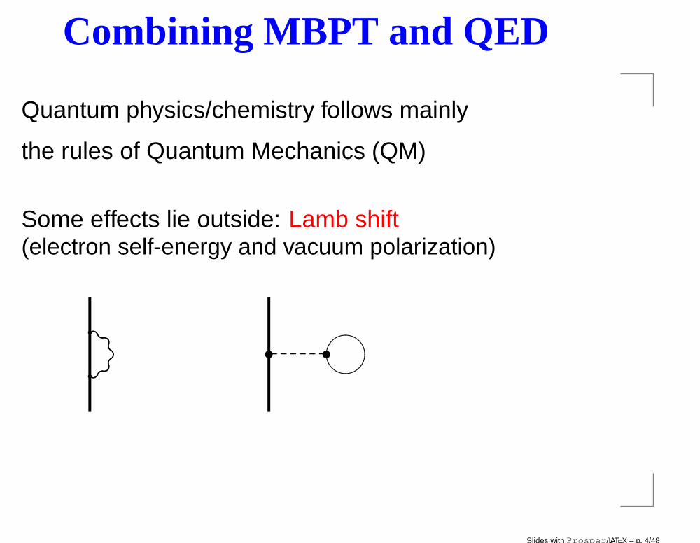
Combining MBPT and QED
Quantum physics/chemistry follows mainly
the rules of Quantum Mechanics (QM)
Some effects lie outside: Lamb shift(electron self-energy and vacuum polarization)
s s
Slides with Prosper/LATEX – p. 4/48
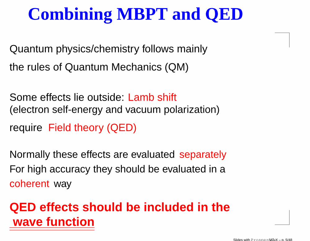
Combining MBPT and QED
Quantum physics/chemistry follows mainly
the rules of Quantum Mechanics (QM)
Some effects lie outside: Lamb shift(electron self-energy and vacuum polarization)
require Field theory (QED)
Normally these effects are evaluated separatelyFor high accuracy they should be evaluated in acoherent way
QED effects should be included in thewave function
Slides with Prosper/LATEX – p. 5/48
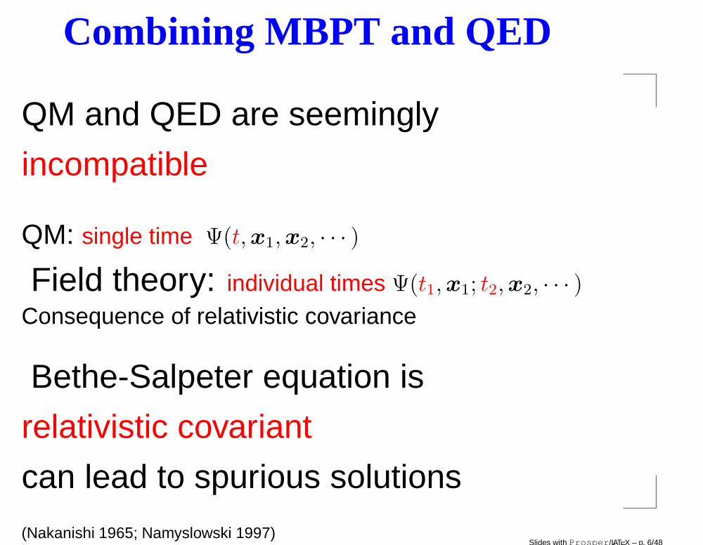
Combining MBPT and QED
QM and QED are seemingly
incompatible
QM: single time Ψ(t,x1,x2, · · · )
Field theory: individual times Ψ(t1,x1; t2,x2, · · · )
Consequence of relativistic covariance
Bethe-Salpeter equation is
relativistic covariant
can lead to spurious solutions
(Nakanishi 1965; Namyslowski 1997)Slides with Prosper/LATEX – p. 6/48
Combining MBPT and QED
Compromise:
Equal-time approximationAll particles given the same time
makes FT compatible with QM
Some sacrifice of the full covariance
very small effect at atomic energies
Slides with Prosper/LATEX – p. 7/48
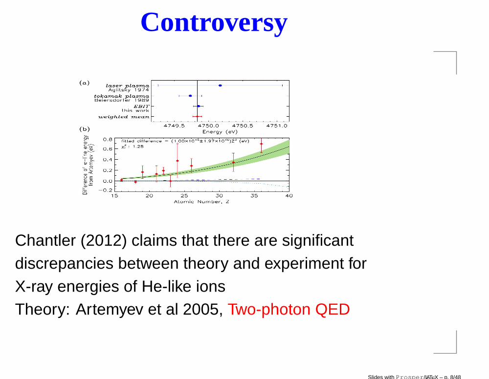
Controversy
Chantler (2012) claims that there are significantdiscrepancies between theory and experiment forX-ray energies of He-like ionsTheory: Artemyev et al 2005, Two-photon QED
Slides with Prosper/LATEX – p. 8/48
Higher-order QED
Higher -order QED can be evaluated by means of theprocedure for
combining QED and MBPT using theGreen’s operator,
a procedure for time-dependent perturbation theory
Slides with Prosper/LATEX – p. 9/48
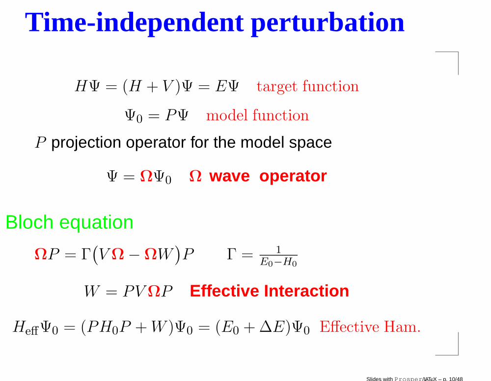
Time-independent perturbation
HΨ = (H + V )Ψ = EΨ target function
Ψ0 = PΨ model function
P projection operator for the model space
Ψ = ΩΨ0 Ω wave operator
Bloch equation
ΩP = Γ(
VΩ−ΩW)
P Γ = 1E0−H0
W = PVΩP Effective Interaction
HeffΨ0 = (PH0P +W )Ψ0 = (E0 +∆E)Ψ0 Effective Ham.
Slides with Prosper/LATEX – p. 10/48
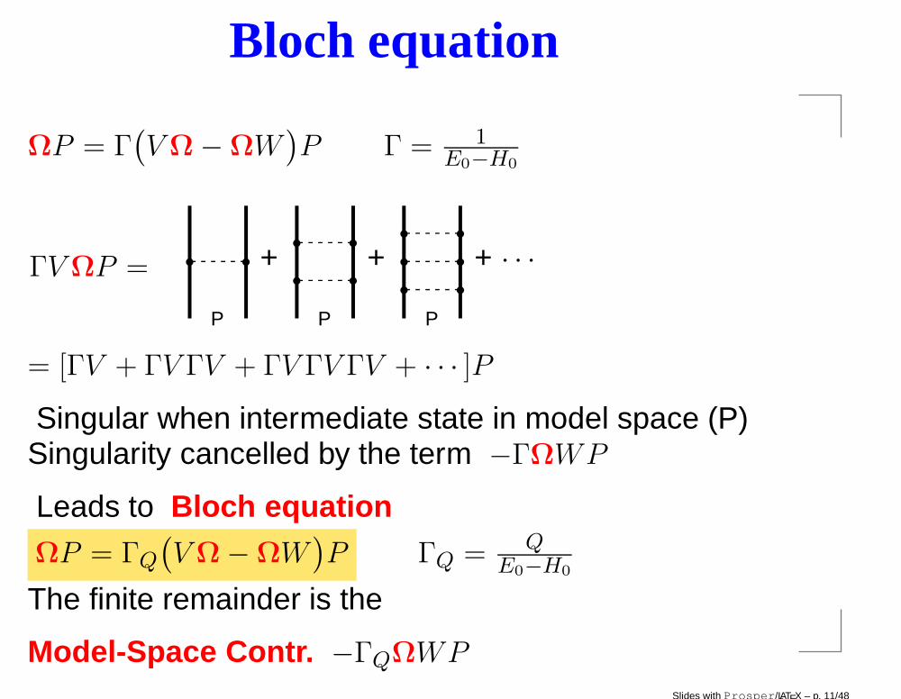
Bloch equation
ΩP = Γ(
VΩ−ΩW)
P Γ = 1E0−H0
r r +
P
ΓVΩP = r rr r
+
P
r rr rr r
+ · · ·
P
= [ΓV + ΓV ΓV + ΓV ΓV ΓV + · · · ]P
Singular when intermediate state in model space (P)Singularity cancelled by the term −ΓΩWP
Leads to Bloch equationΩP = ΓQ
(
VΩ−ΩW)
P ΓQ = QE0−H0
The finite remainder is the
Model-Space Contr. −ΓQΩWP
Slides with Prosper/LATEX – p. 11/48
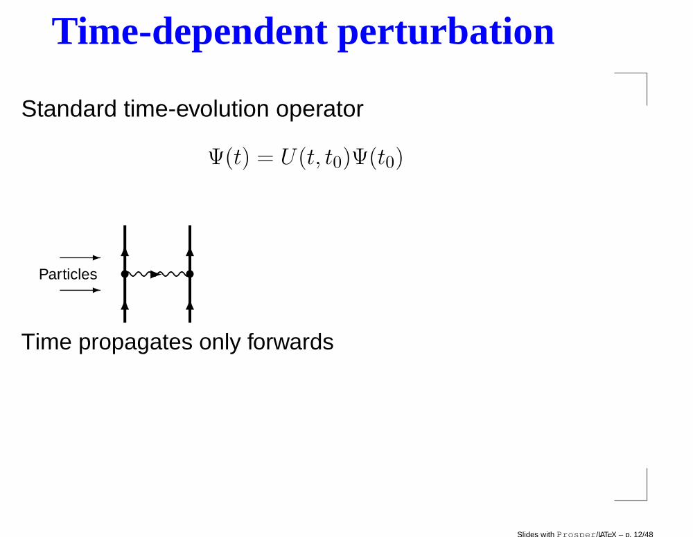
Time-dependent perturbation
Standard time-evolution operator
Ψ(t) = U(t, t0)Ψ(t0)
s s
Particles
Time propagates only forwards
Slides with Prosper/LATEX – p. 12/48
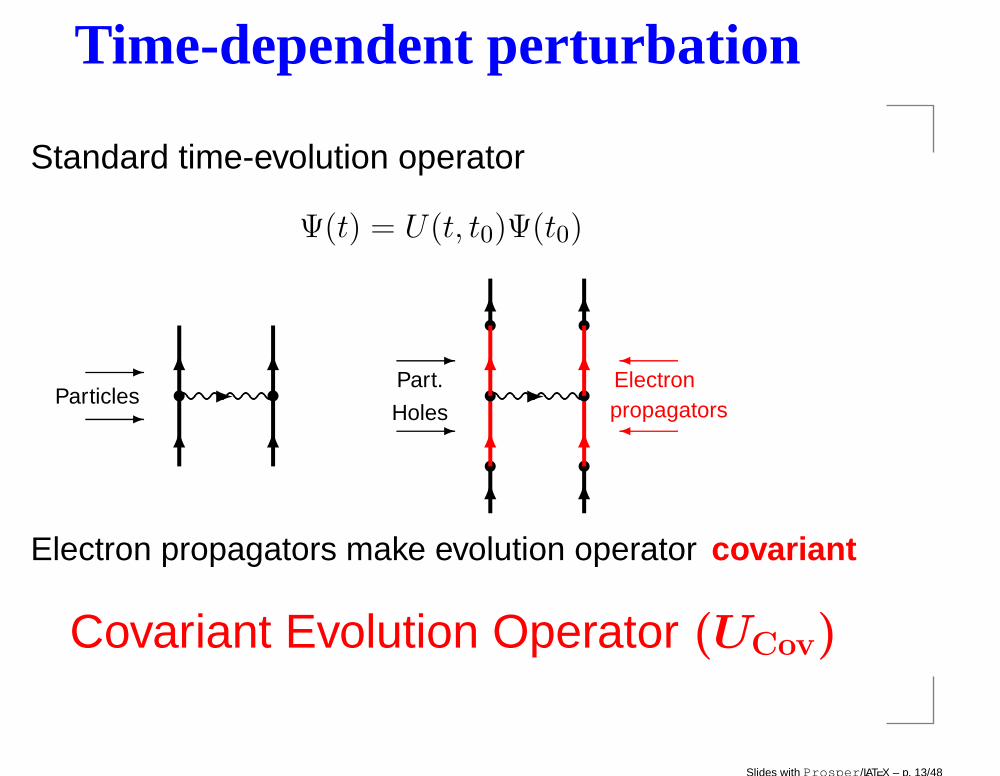
Time-dependent perturbation
Standard time-evolution operator
Ψ(t) = U(t, t0)Ψ(t0)
s s
Particles
s s
s s
s s
Part.
Holes
Electronpropagators
Electron propagators make evolution operator covariant
Covariant Evolution Operator (UCov)
Slides with Prosper/LATEX – p. 13/48
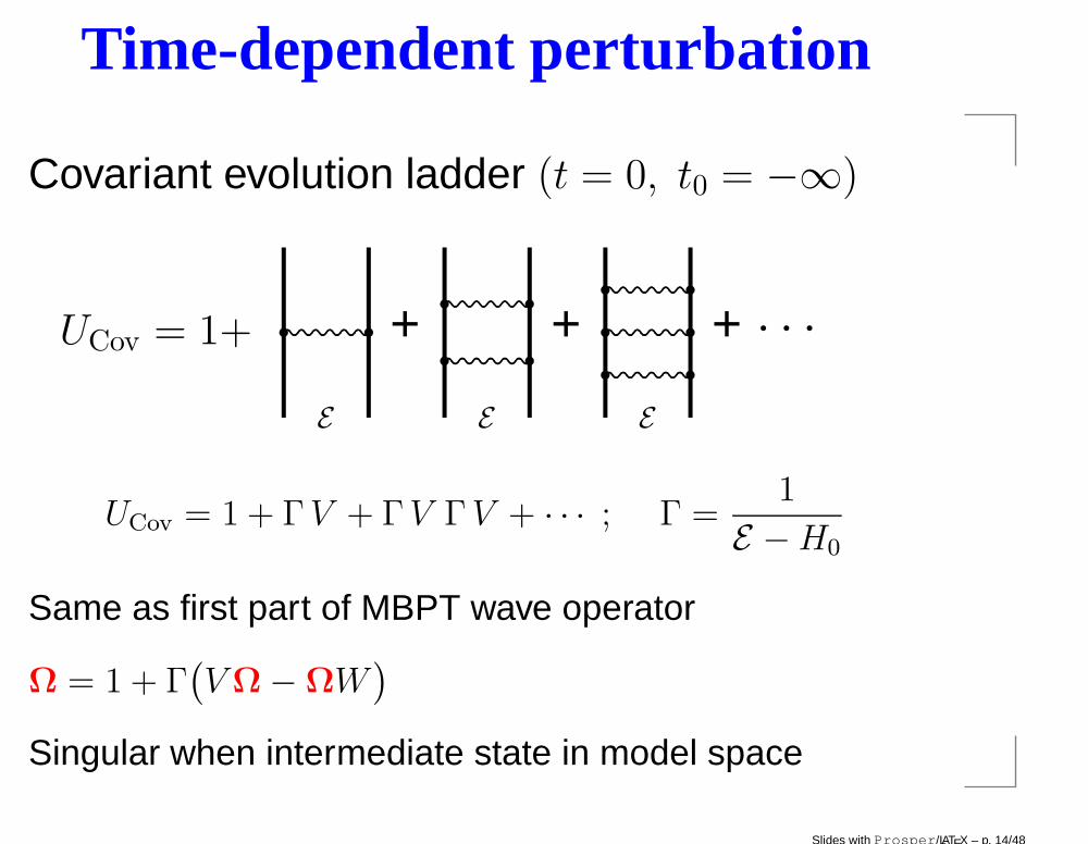
Time-dependent perturbation
Covariant evolution ladder (t = 0, t0 = −∞)
UCov = 1+ r r
E
+ r rr r
+
E
r rr rr r
+ · · ·
E
UCov = 1 + ΓV + ΓV ΓV + · · · ; Γ =1
E −H0
Same as first part of MBPT wave operator
Ω = 1 + Γ(
VΩ−ΩW)
Singular when intermediate state in model space
Slides with Prosper/LATEX – p. 14/48
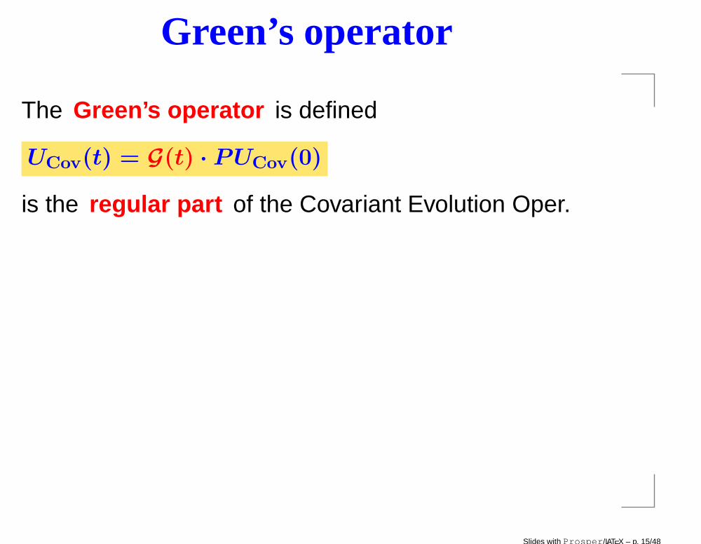
Green’s operator
The Green’s operator is defined
UCov(t) = G(t) · PUCov(0)
is the regular part of the Covariant Evolution Oper.
Slides with Prosper/LATEX – p. 15/48
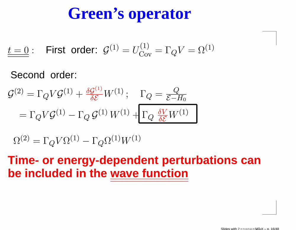
Green’s operator
t = 0 : First order: G(1) = U(1)Cov = ΓQV = Ω(1)
Second order:
G(2) = ΓQV G(1) + δG(1)
δEW (1) ; ΓQ = Q
E−H0
= ΓQV G(1) − ΓQ G(1)W (1) + ΓQδVδE
W (1)
Ω(2) = ΓQV Ω(1) − ΓQΩ(1)W (1)
Time- or energy-dependent perturbations canbe included in the wave function
Slides with Prosper/LATEX – p. 16/48
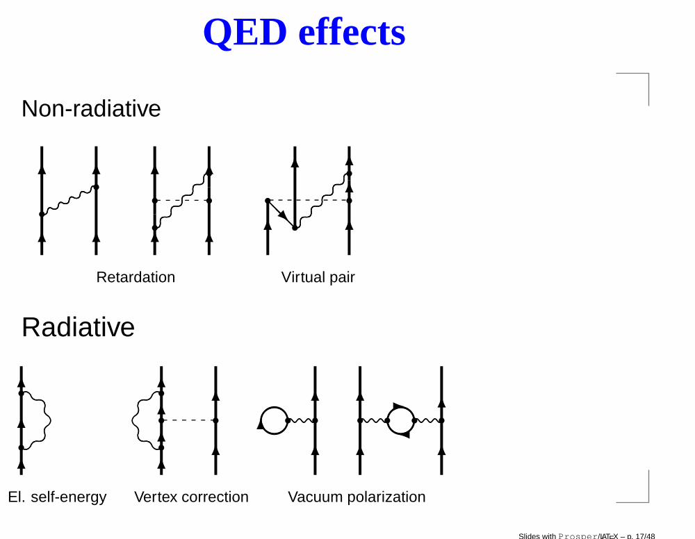
QED effects
Non-radiative
rr
Retardation
r
r
r r
r r
r
r
Virtual pair
Radiative
r
r
El. self-energy
r
rr r
Vertex correction
♠♠♠♠♠
r r
Vacuum polarization
r r ♠♠♠♠♠r r
Slides with Prosper/LATEX – p. 17/48
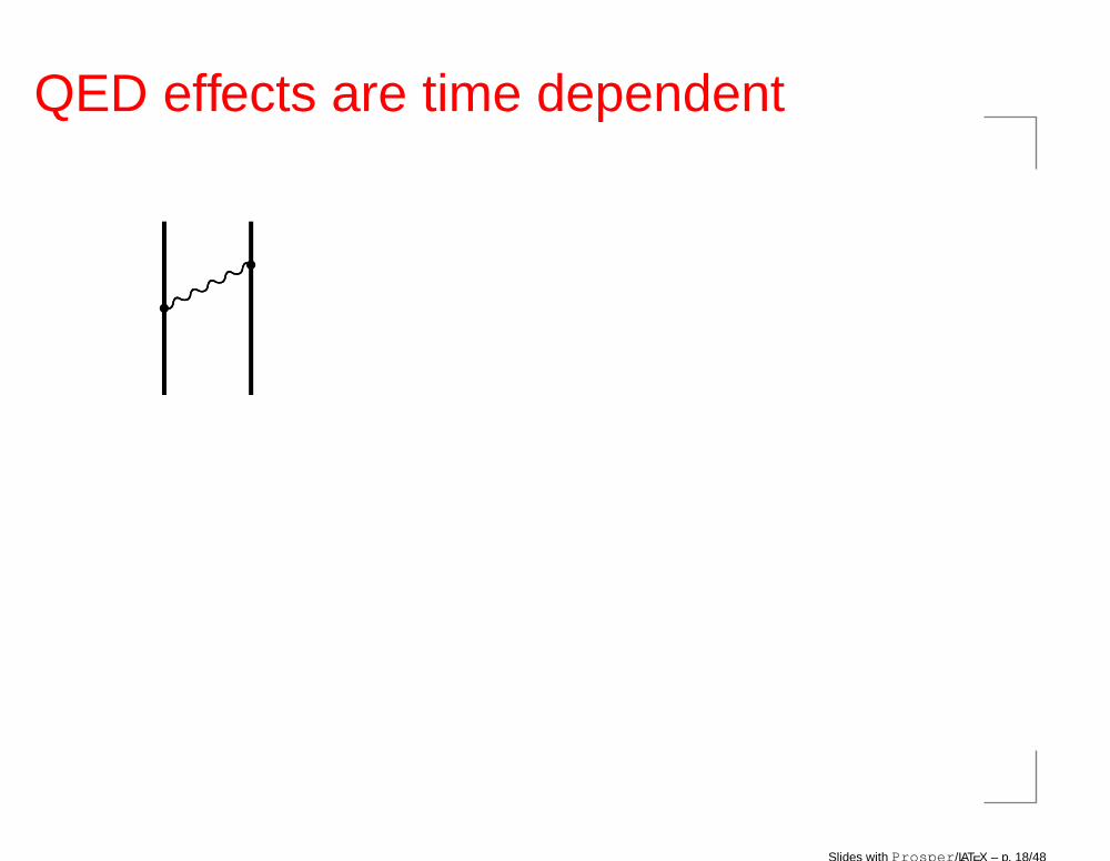
QED effects are time dependent
rr
Slides with Prosper/LATEX – p. 18/48
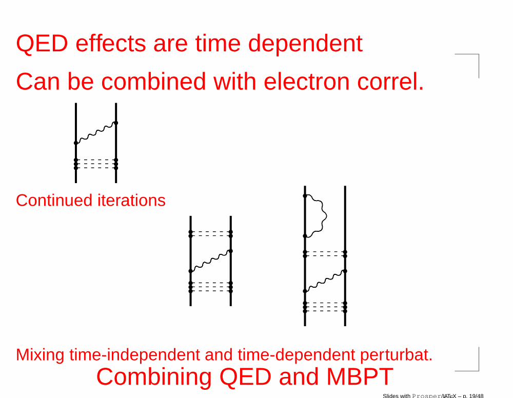
QED effects are time dependent
Can be combined with electron correl.
rr
r rr rr r
Continued iterations
rr
r rr rr r
r rr r
rr
r rr rr r
r rr rr
r
Mixing time-independent and time-dependent perturbat.
Combining QED and MBPTSlides with Prosper/LATEX – p. 19/48
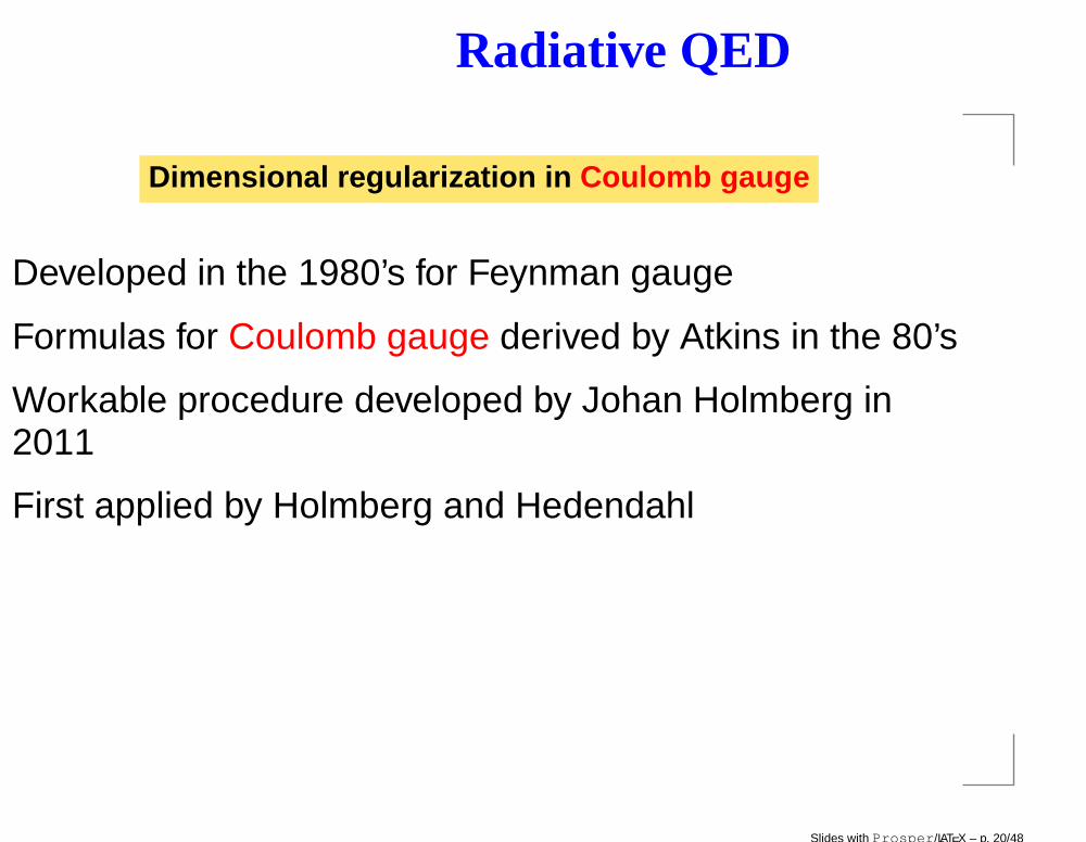
Radiative QED
Dimensional regularization in Coulomb gauge
Developed in the 1980’s for Feynman gauge
Formulas for Coulomb gauge derived by Atkins in the 80’s
Workable procedure developed by Johan Holmberg in2011
First applied by Holmberg and Hedendahl
Slides with Prosper/LATEX – p. 20/48
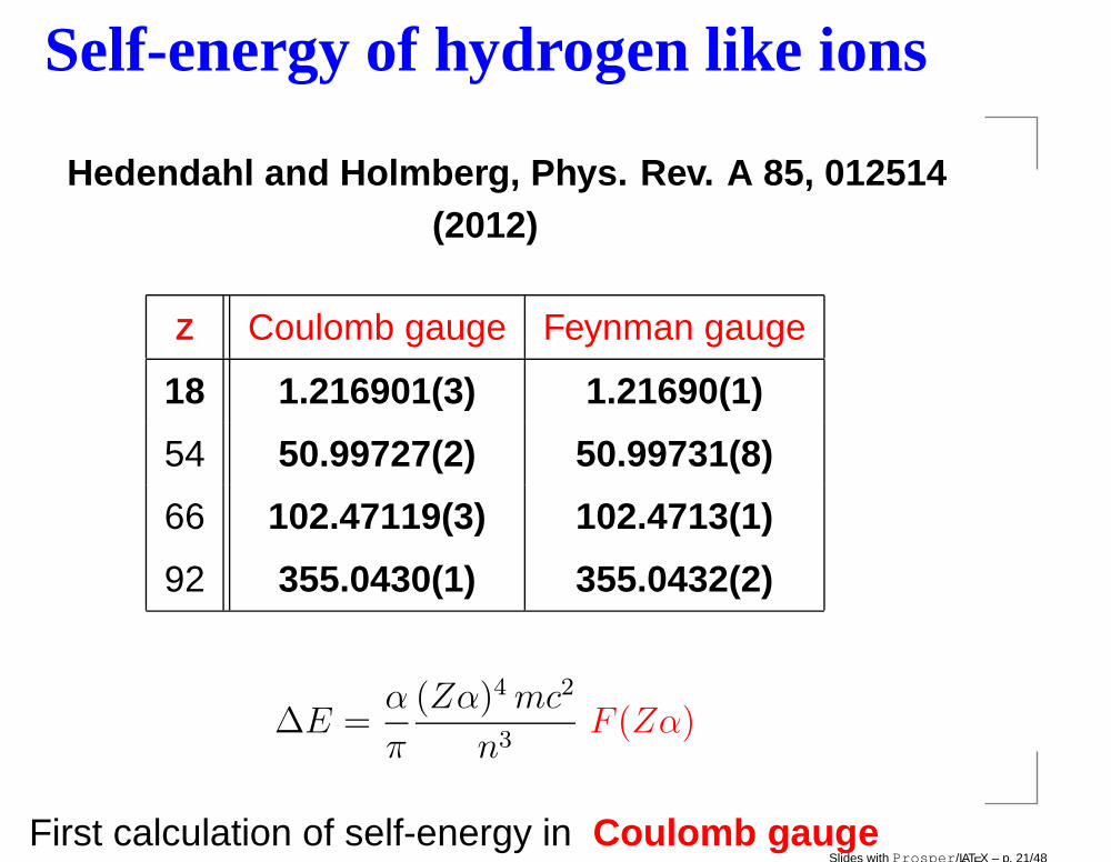
Self-energy of hydrogen like ions
Hedendahl and Holmberg, Phys. Rev. A 85, 012514(2012)
Z Coulomb gauge Feynman gauge
18 1.216901(3) 1.21690(1)
54 50.99727(2) 50.99731(8)
66 102.47119(3) 102.4713(1)
92 355.0430(1) 355.0432(2)
∆E =α
π
(Zα)4mc2
n3F (Zα)
First calculation of self-energy in Coulomb gaugeSlides with Prosper/LATEX – p. 21/48
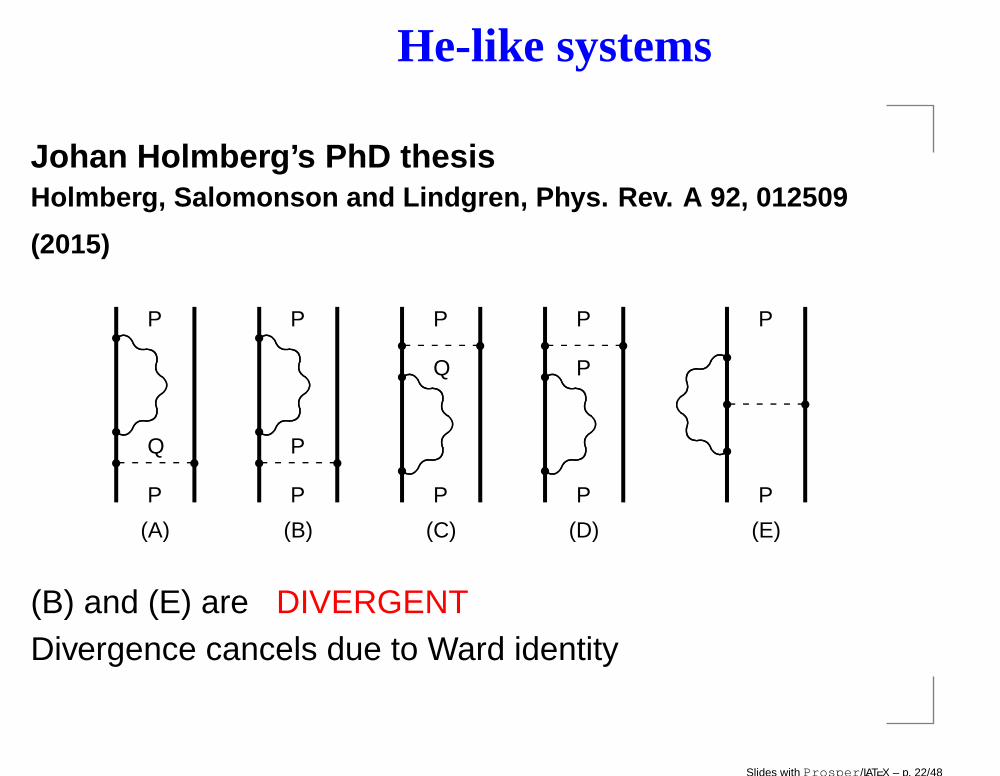
He-like systems
Johan Holmberg’s PhD thesisHolmberg, Salomonson and Lindgren, Phys. Rev. A 92, 012509
(2015)
r
r
r rP
Q
P
(A)
r
r
r rP
P
P
(B)
r
rr r
P
Q
P
(C)
r
rr r
P
P
P
(D)
r
rr r
P
P
(E)
(B) and (E) are DIVERGENTDivergence cancels due to Ward identity
Slides with Prosper/LATEX – p. 22/48
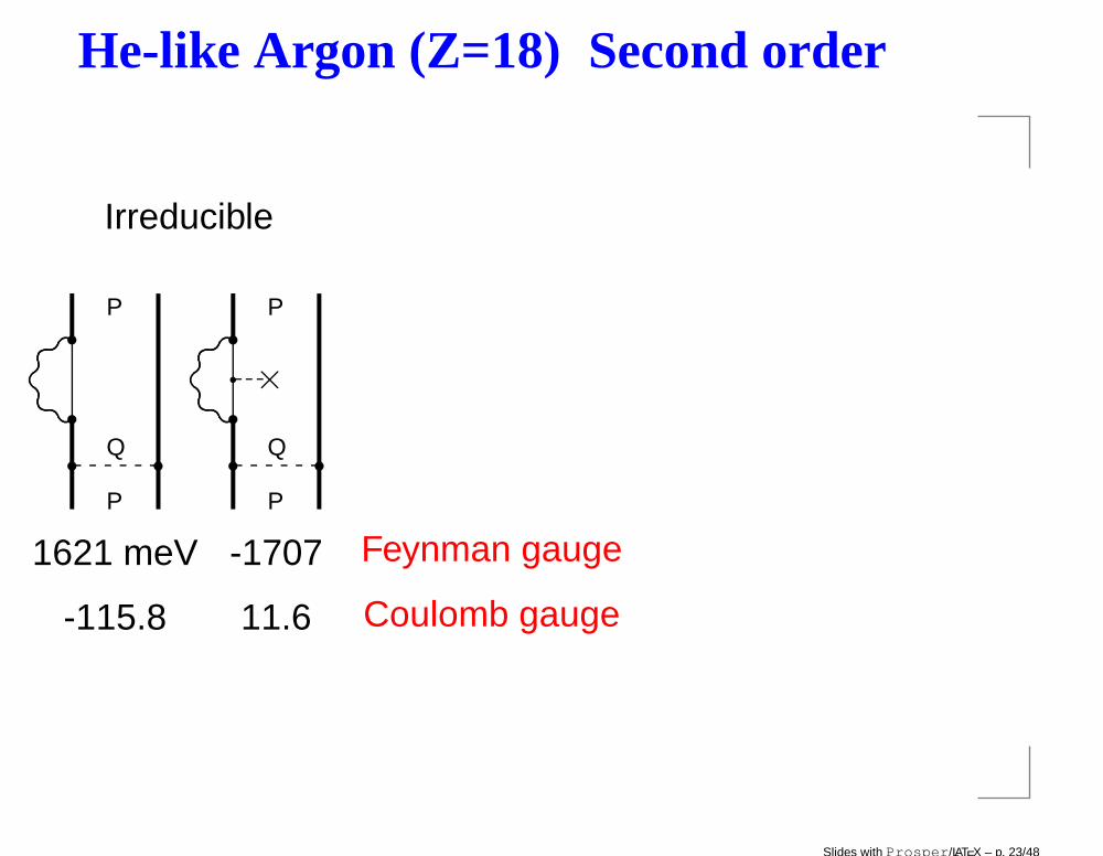
He-like Argon (Z=18) Second order
Irreducible
r
r
r rP
Q
P
1621 meV
-115.8
r
r×q
r rP
Q
P
-1707
11.6
Feynman gauge
Coulomb gauge
Slides with Prosper/LATEX – p. 23/48
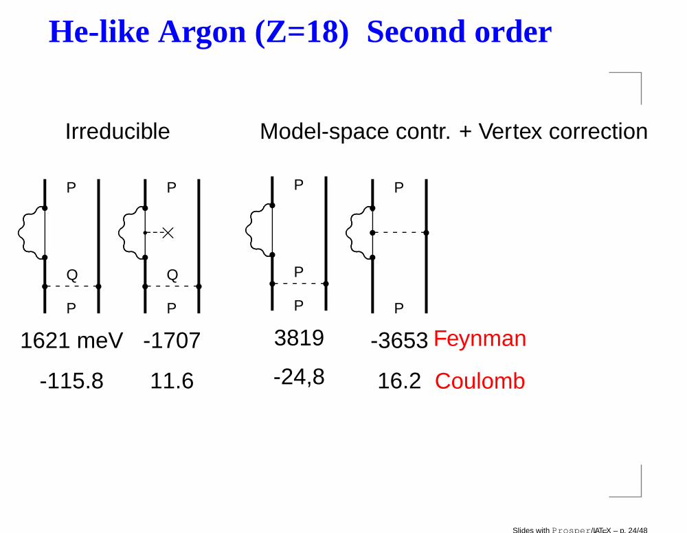
He-like Argon (Z=18) Second order
Irreducible Model-space contr. + Vertex correction
r
r
r rP
Q
P
1621 meV
-115.8
r
r×q
r rP
Q
P
-1707
11.6
r
r
r rP
P
P
3819
-24,8
r
rr r
P
-3653
16.2
P
Feynman
Coulomb
Slides with Prosper/LATEX – p. 24/48
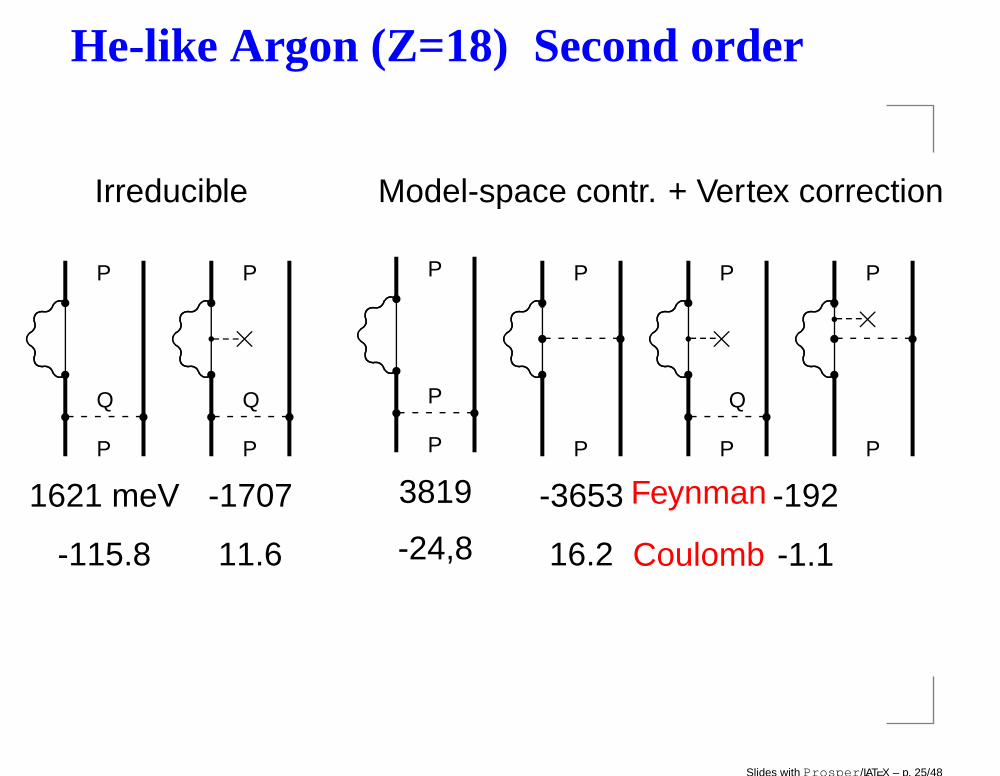
He-like Argon (Z=18) Second order
Irreducible Model-space contr. + Vertex correction
r
r
r rP
Q
P
1621 meV
-115.8
r
r×q
r rP
Q
P
-1707
11.6
r
r
r rP
P
P
3819
-24,8
r
rr r
P
-3653
16.2
P
Feynman
Coulomb
r
r×q
r rP
Q
P
-192
-1.1
r
r×qr r
P
P
Slides with Prosper/LATEX – p. 25/48
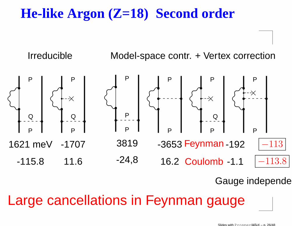
He-like Argon (Z=18) Second order
Irreducible Model-space contr. + Vertex correction
r
r
r rP
Q
P
1621 meV
-115.8
r
r×q
r rP
Q
P
-1707
11.6
r
r
r rP
P
P
3819
-24,8
r
rr r
P
-3653
16.2
P
Feynman
Coulomb
r
r×q
r rP
Q
P
-192
-1.1
r
r×qr r
P
P
−113
−113.8
Gauge independent
Large cancellations in Feynman gauge
Slides with Prosper/LATEX – p. 26/48
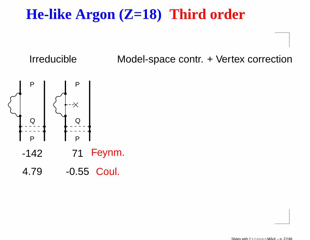
He-like Argon (Z=18) Third order
Irreducible Model-space contr. + Vertex correction
r
r
r rr rP
Q
P
-142
4.79
r
r×q
r rr rQ
P
P
71
-0.55
Feynm.
Coul.
Slides with Prosper/LATEX – p. 27/48
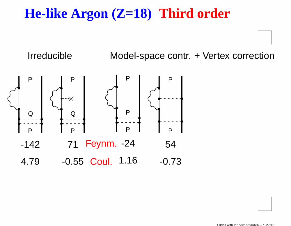
He-like Argon (Z=18) Third order
Irreducible Model-space contr. + Vertex correction
r
r
r rr rP
Q
P
-142
4.79
r
r×q
r rr rQ
P
P
71
-0.55
Feynm.
Coul.
r
r
r rr rP
P
P
-24
1.16
r
rr r
r rP
P
54
-0.73
Slides with Prosper/LATEX – p. 27/48
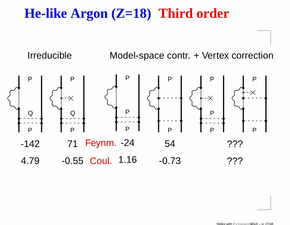
He-like Argon (Z=18) Third order
Irreducible Model-space contr. + Vertex correction
r
r
r rr rP
Q
P
-142
4.79
r
r×q
r rr rQ
P
P
71
-0.55
Feynm.
Coul.
r
r
r rr rP
P
P
-24
1.16
r
rr r
r rP
P
54
-0.73
r
r×q
r rr rP
P
P
???
???
r
r×qr r
r rP
P
Slides with Prosper/LATEX – p. 27/48
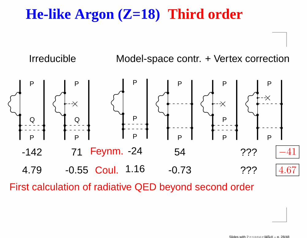
He-like Argon (Z=18) Third order
Irreducible Model-space contr. + Vertex correction
r
r
r rr rP
Q
P
-142
4.79
r
r×q
r rr rQ
P
P
71
-0.55
Feynm.
Coul.
r
r
r rr rP
P
P
-24
1.16
r
rr r
r rP
P
54
-0.73
r
r×q
r rr rP
P
P
???
???
r
r×qr r
r rP
P
−41
4.67
First calculation of radiative QED beyond second order
Slides with Prosper/LATEX – p. 28/48
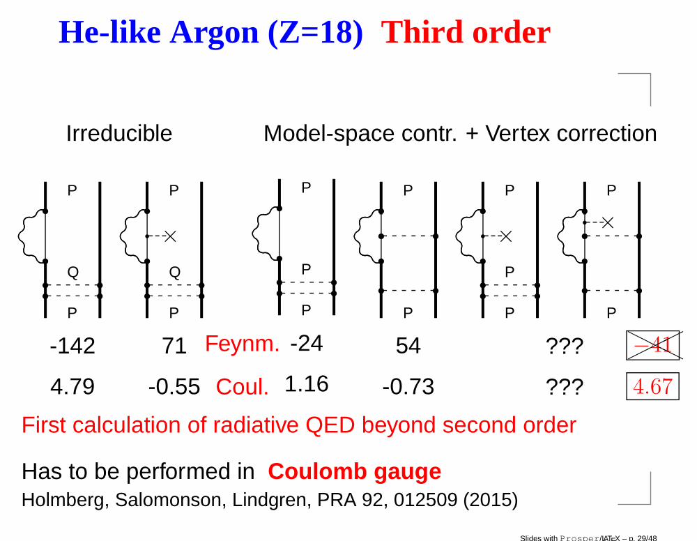
He-like Argon (Z=18) Third order
Irreducible Model-space contr. + Vertex correction
r
r
r rr rP
Q
P
-142
4.79
r
r×q
r rr rQ
P
P
71
-0.55
Feynm.
Coul.
r
r
r rr rP
P
P
-24
1.16
r
rr r
r rP
P
54
-0.73
r
r×q
r rr rP
P
P
???
???
r
r×qr r
r rP
P
−41
4.67
First calculation of radiative QED beyond second order
Has to be performed in Coulomb gaugeHolmberg, Salomonson, Lindgren, PRA 92, 012509 (2015)
Slides with Prosper/LATEX – p. 29/48
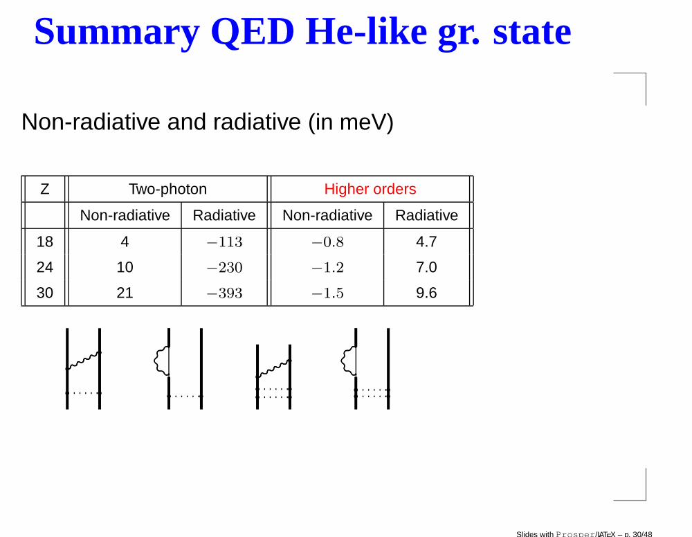
Summary QED He-like gr. state
Non-radiative and radiative (in meV)
Z Two-photon Higher orders
Non-radiative Radiative Non-radiative Radiative
18 4 −113 −0.8 4.7
24 10 −230 −1.2 7.0
30 21 −393 −1.5 9.6
q qq q ♣
♣
q qq qq qq q ♣
♣
q qq q
Slides with Prosper/LATEX – p. 30/48
Summary QED He-like gr. state
Higher-order QED (in meV)
Z Holmberg 2015 (calc) Artemyev 2005 (est’d)
14 1.6 (2) 0.8
18 2.0 (3) 0.9
24 3.9 (5)
30 5.6 (8) −0.2
50 12 (2) −7.7(50)
Chantler
500 meV
Slides with Prosper/LATEX – p. 31/48
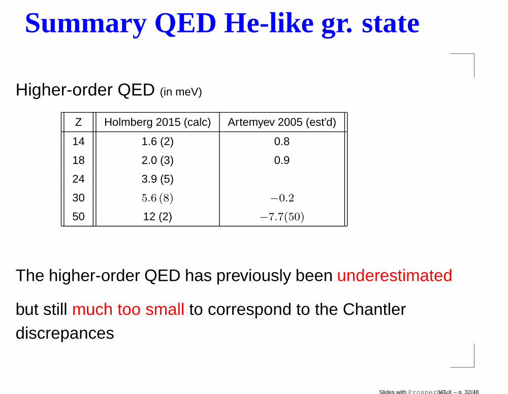
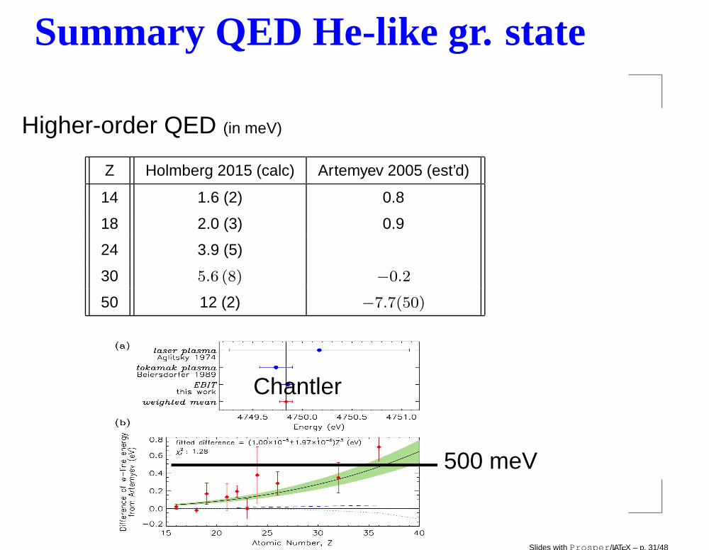
Summary QED He-like gr. state
Higher-order QED (in meV)
Z Holmberg 2015 (calc) Artemyev 2005 (est’d)
14 1.6 (2) 0.8
18 2.0 (3) 0.9
24 3.9 (5)
30 5.6 (8) −0.2
50 12 (2) −7.7(50)
The higher-order QED has previously been underestimated
but still much too small to correspond to the Chantlerdiscrepances
Slides with Prosper/LATEX – p. 32/48
Dynamical processes
The Green’s operator can also be used
in dynamical processes
Slides with Prosper/LATEX – p. 33/48
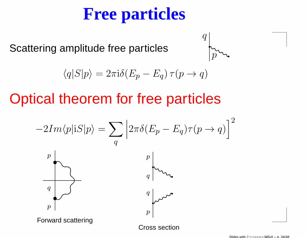
Free particles
Scattering amplitude free particles qqqp
〈q|S|p〉 = 2πiδ(Ep − Eq) τ(p → q)
Optical theorem for free particles
−2Im〈p|iS|p〉 =∑
q
∣
∣
∣2πδ(Ep − Eq)τ(p → q)
]2
s
s
q
p
p
Forward scattering
p
q
p
q
Cross sectionSlides with Prosper/LATEX – p. 34/48
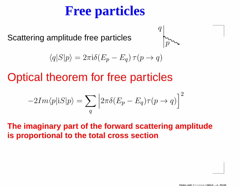
Free particles
Scattering amplitude free particles qqqp
〈q|S|p〉 = 2πiδ(Ep − Eq) τ(p → q)
Optical theorem for free particles
−2Im〈p|iS|p〉 =∑
q
∣
∣
∣2πδ(Ep − Eq)τ(p → q)
]2
The imaginary part of the forward scattering amplitudeis proportional to the total cross section
Slides with Prosper/LATEX – p. 35/48
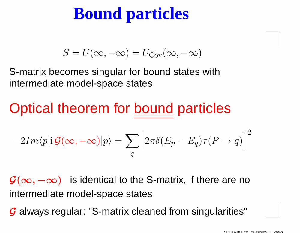
Bound particles
S = U(∞,−∞) = UCov(∞,−∞)
S-matrix becomes singular for bound states withintermediate model-space states
Optical theorem for bound particles
−2Im〈p|iG(∞,−∞)|p〉 =∑
q
∣
∣
∣2πδ(Ep − Eq)τ(P → q)
]2
G(∞,−∞) is identical to the S-matrix, if there are nointermediate model-space states
G always regular: "S-matrix cleaned from singularities"
Slides with Prosper/LATEX – p. 36/48
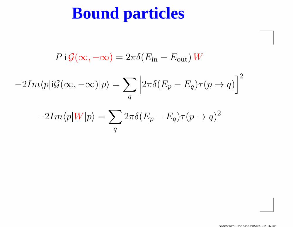
Bound particles
P iG(∞,−∞) = 2πδ(Ein − Eout)W
−2Im〈p|iG(∞,−∞)|p〉 =∑
q
∣
∣
∣2πδ(Ep − Eq)τ(p → q)
]2
−2Im〈p|W |p〉 =∑
q
2πδ(Ep − Eq)τ(p → q)2
Slides with Prosper/LATEX – p. 37/48
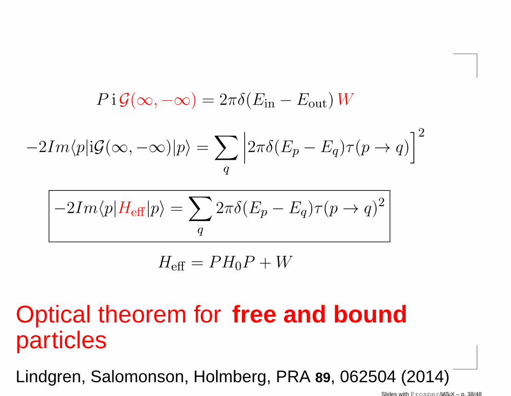
P iG(∞,−∞) = 2πδ(Ein − Eout)W
−2Im〈p|iG(∞,−∞)|p〉 =∑
q
∣
∣
∣2πδ(Ep − Eq)τ(p → q)
]2
−2Im〈p|Heff |p〉 =∑
q
2πδ(Ep − Eq)τ(p → q)2
Heff = PH0P +W
Optical theorem for free and boundparticlesLindgren, Salomonson, Holmberg, PRA 89, 062504 (2014)
Slides with Prosper/LATEX – p. 38/48
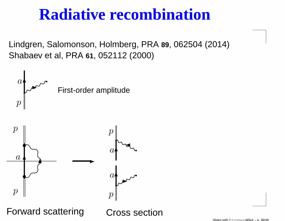
Radiative recombination
Lindgren, Salomonson, Holmberg, PRA 89, 062504 (2014)Shabaev et al, PRA 61, 052112 (2000)
qqa
p
First-order amplitude
a
s
s
p
p
Forward scattering
a q
q
qqa
p
p
Cross sectionSlides with Prosper/LATEX – p. 39/48
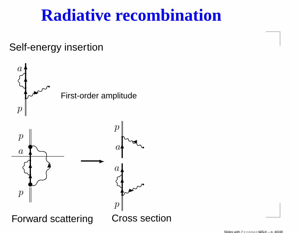
Radiative recombination
Self-energy insertion
qqa
p
First-order amplitude
t
t
a
p
p
Forward scattering
a q
q
♣♣a
p
p
Cross sectionSlides with Prosper/LATEX – p. 40/48
Radiative recombination
Self-energy insertion leads to singularity
that is taken care of in the Green’s operator.
Slides with Prosper/LATEX – p. 41/48
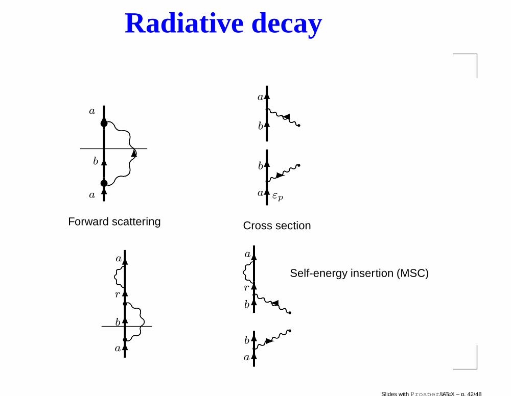
Radiative decay
b
t
ta
a
Forward scattering
a
b q
q
a
b
εp
Cross section
a
a
b
r
r
r♣♣
a
r
a
b
b
qq♣♣
Self-energy insertion (MSC)
Slides with Prosper/LATEX – p. 42/48
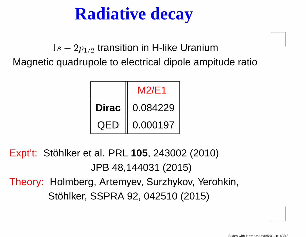
Radiative decay
1s− 2p1/2 transition in H-like UraniumMagnetic quadrupole to electrical dipole ampitude ratio
M2/E1
Dirac 0.084229
QED 0.000197
Expt’t: Stöhlker et al. PRL 105, 243002 (2010)JPB 48,144031 (2015)
Theory: Holmberg, Artemyev, Surzhykov, Yerohkin,Stöhlker, SSPRA 92, 042510 (2015)
Slides with Prosper/LATEX – p. 43/48
Conclusions and Outlook
The Green’s operator is atime-dependent wave operator
Can combine time-dependent and time-independentperturbations, unifying QED and MBPT
Can be used for stationary as well as dynamicalproblems (real and imaginary parts, respectively)
Improves the accuracy of theoretical estimatesone order of magnitude
Slides with Prosper/LATEX – p. 44/48
Conclusions and Outlook
The Green’s operator
has been used to evaluate QED beyond second order,employing Coulomb gauge for radiative QED
applied to dynamical problems to derive
the Optical Theorem for bound systems
to evaluate the QED effect in radiative recombinationand in radiative decay (together with GSI, Jena)
Slides with Prosper/LATEX – p. 45/48

This work has been supported by
The Swedish Science Reseach Council
The Humboldt Foundation
Helmholtz Association
Gesellschaft für Schwerionenforschung
Slides with Prosper/LATEX – p. 46/48

Thank you!
Slides with Prosper/LATEX – p. 47/48
Slides with Prosper/LATEX – p. 48/48