Uniformity of Dosage Units, Part 1: Acceptance Valuefiles.pharmtech.com/alfresco_images/pharma/2018/11/... · Table I: Current vs. new acceptance value (AV) formulas and how they’re

30 Pharmaceutical Technology November 2018 PharmTech .com

EL

RE

PH

O/S

TO

CK

.AD

OB

E.C

OM

Peer-Reviewed

In methods currently used to ensure the uniformity of dosage units (UDU) (1), the test acceptance value (AV) is based on the following formula: AV = M x + ks, where M is reference value, x is sample mean, k is acceptability constant, and s is sample

standard deviation.Despite its widespread use, this method can result in bias and

may allow batches of inferior quality to be released. The bias can result in fluctuated conclusions, especially when guidance established by the American Society for Testing and Materials’ (ASTM) E2810 standard guide (2) is followed. Studies have found lack of correlation between AV and probability (ASTM E2810) computed using validation data. In addition, AV, as it is typically computed, is also inconsistent with lot coverage (3). This incon-sistency is caused by the conditional determination criteria that are used to determine the reference value (M).

In order to remove bias from the AV limit, the definition of M must be adjusted. One way to do this is by replacing it with the process target (T). Appropriate derivation using statistical techniques can result in an unbiased formula with increased dis-criminative power to generate a new AV distribution. Using this approach, the higher power would be indicated by one AV limit for each sample size, for example, as well as one limit for each target, and limitation of “T-Xbar” values, effectively preventing the release of inferior quality batches.

Critical AV values (at locations with 95% or 99% coverage) can be determined after simulation studies and complete construc-tion of the distributions, so that new and unbiased AV limits can be established. This article will briefly describe how to do this.

The test acceptance criteria for current (UDU) (1) are sum-marized as follows, where AV = acceptance value, M = reference value, s = standard deviation, x = content uniformity data mean, xmin = minimum, and xmax = maximum of 30 units:

• Stage 1: assay 10 units. Pass if AV = M x + 2.4s 15 criteria are met.• Stage 2: assay 20 additional units. Pass if AV = M x + 2s 15 criteria

are met, provided that xmin ≥ 0.75M and xmax ≤ 1.25M criteria are also met.

The determination criteria for reference value (M) are subject to the target value (T), which may be not more than 101.5% of the label claim (LC) (where M may be x, 98.5 or 101.5% LC) or more than 101.5% LC (where M may be x, 98.5 or T% LC). See United States Pharmacopeia (USP) (1) for more detail.

The concept of acceptance value must be redefined to remove bias and more closely reflect quality targets. This paper describes how this can be done.

Uniformity of Dosage Units, Part 1: Acceptance ValuePramote Cholayudth

Submitted: June 12, 2018Accepted: July 20, 2018

Pramote Cholayudth is validation consultant to Biolab Co., Ltd. in Thailand. He is a guest speaker on process validation to industrial pharmaceutical scientists organized by local regulatory authorities. He is the founder and manager of PM Consult and can be contacted via [email protected].


Peer-Reviewed

AL

L F

IGU

RE

S A

RE

CO

UR

TE

SY

OF

TH

E A

UT

HO

R.

A previous study (4, 5, 6) suggests that AV values are not always consistent with reliability, so they cannot fully guar-antee that the batches being tested meet UDU. According to part three of that study (6), the definition of the AV for-mula, AV = M x + ks, where AV is acceptance value, M is refer-ence value, x is sample mean, s is sample standard deviation, and k is acceptability constant, is the root cause of the bias since it is associated with the biased determination criteria. For example, the previous formula forces M for any samples with means less than 98.5% or more than 101.5% LC to be 98.5 or 101.5% LC, respectively (when the target is not more than 101.5% LC).

The following (see Figure 1) is a relevant example of errors (6). Figure 1 illustrates lack of correlation between AV and probability graphs (according to ASTM E2810) due to its non-linearity. The probability pitfalls at 98.5% and 101.5% LC mean locations illus-trate how the formula influences the AV parameter’s reliability.

Use of the working AV limits (6) (e.g., not more than [NMT] 12.5 for n = 10) still has a limitation (i.e., its validity exists only when sample mean values are those other than 98.5% or 101.5% LC). For 91.13% probability, as shown in the figure,

there is 90% assurance (a 90% joint confidence interval) that at least 91.13% of all samples tested for content uniformity will pass the USP test.

The new concept of acceptance value (AV)To remove the discriminative power bias and subsequently fix the method currently used to establish AV limits, the definition of M needs to be adjusted through directly using the process target (T). In order for the formula to be unbiased and more discriminative, it must divide by the square root of sample size n (i.e., in the same manner used to determine the standard error of the mean, σ∕√n) so that it is a function of sample size. Taking this approach, the current formula (Equation 1)

AV = M x + ks [Eq. 1]

would become the following expression (Equation 2),

AV = T x / n +ks [Eq. 2]

Simulation studies must be run, however, to confirm the va-lidity of this hypothesis.

An appendix to part one of the study mentioned previously (4), describes the statistical methods that are used, which include deriving the probability density function (pdf) formula in-volved. Since the overall approach will be exactly the same as that used in the previous study (4), it may be sufficient to compare current AV numbers with derivations using the new AV formula derivation. This comparison is shown in Table I. When using the Microsoft Excel formula (Equation 3):

Probability (P) = CHISQ.DIST(x,n - 1,TRUE) [Eq. 3]

where, for practical use, chi variable χ2 is now replaced by x vari-able. In Table I and Equation 3,

• χ2 is the Chi-square variable (it is a numerical variable equiv-alent to each of the AV data on the x-axis)

Figure 1: The relationship among critical acceptance values (AVs), probability, and mean value for content uniformity (CU) (validation sample size n = 30).

Table I: Current vs. new acceptance value (AV) formulas and how they’re derived.Current acceptance value New acceptance value

• To create the new formula, the reference value M in the current formula is replaced with the target value, T. To make the formula discriminative, it needs to be divisible by the square root of the sample size n, in the same manner as the expression for the standard error of the mean, / n .

Current AV formula: AV = M x +ks New AV formula: AV = T x / n +ks

• To create the probability density function (pdf) using chi square statistics (4), the average value M x in the current chi square formula must be replaced with the average value T x / n (where T x = 0.94748 in cell “G2” in Table II). The only difference is the average values. This is why the approach remains the same.

Current χ2 formula:

2 =(μ / )2 +1

1/ n 1k2μ2

AV M x2

+1/ n New χ2 formula:

2 =(μ / )2 +1

1/ n 1k2μ2

AV T x / n2

+1/ n

For more detail, see reference 4. In Excel format, see cell “G4” in Table II.

• From the χ2 formula: To generate the probability density using the corresponding chi square function in MS Excel, the same formula must be used for both current and new, i.e. Probability (P) = CHISQ.DIST(χ2,n-1,TRUE) or CHISQ.DIST(x,n-1,TRUE) see Equation 3 above. See also cell “G5” in Table II.

Pharmaceutical Technology November 2018 33

• n is sample size• n-1 is n-1 degrees of freedom• μ is process mean (mu)• σ is process standard deviation (sigma)• AV is acceptance value (on x-axis)

• M is reference value• T is target value• x is sample mean• k is acceptability constant• M x is absolute value between reference value (M) and sample

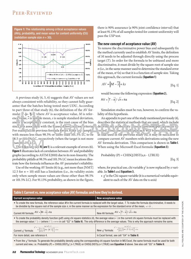
Table II: New acceptance value (AV) vs. probability data (n = 10) (Microsoft Excel spreadsheet). ABS is the absolute function in Microsoft Excel.

A B C D E F G H I

1Descriptions

n Mean Sigma (T-Xbar) av. Lot CpK K

2 10 100.00 3.75 0.94748 1.33 2.40

3 New AV data (x-axis) 6.00 6.25 6.50 6.75 7.00 7.25

4 Chi square variable 3.61 3.94 4.28 4.63 4.99 5.37

5 Probability density (cumulative) 6.50% 8.45% 10.76% 13.44% 16.50% 19.92%

6 Probability density (y-axis) 1.78% 2.13% 2.50% 2.87% 3.24% 3.59%

7 G2 = 0.94748 (the average of all IT-XbarI values generated from the simulation study N = 900,000)

8 H2 = MIN(115-E2,E2-85)/(3 * F2) = 1.33333

9 G3 = F3 + 0.25 = 6.75, H3 = G3+0.25, I3 = H3 + 0.25, and so on

10 G4 = (($E$2/$F$2)^2 + 1)/((1/((($D$2 - 1)/(($I$2*$E$2)^2))*((G3-$G$2/$D$2^0.5)^2)))+(1/$D$2)) = 4.63

11 G5 = CHISQ.DIST(G4,$D$2 - 1,TRUE) = 13.44%

12 G6 = ABS(H5 - F5)/2 = 2.87% (probability density at AV = 6.75)


Peer-Reviewed

mean (x) and M x is the average of all M x data in simulation• T x is absolute value between target value (T) and sample

mean (x) and T x is the average of all T x data in simulation• P is probability density (%) (on y-axis)• CHISQ.DIST is the MS Excel function that will return the

chi square (χ2 or x) distribution (%)• TRUE is the cumulative distribution

Construction of theoretical AV distribution (n = 10)According to part one of the previous study (4), the minimum process capability index, CpK, i.e., Lot CpK at 1.33 (using mean = 100 and sigma = 3.75) is used as a benchmark and the baseline for working AV acceptance limits. The same baseline is also ap-plied in this study.

An Excel function (Equation 3) is used to compute the probability density (% frequency), when the spreadsheet in Table II is keyed with parameters such as n = 10, mean = 100, and sigma = 3.75. In Table II, within thick-line border, if the new AV = 6.75 (x-axis), then the chi-square vari-able = 4.63, and the cumulative probability density will be 13.44%, while the non-cumulative probability density will be 2.87%.

The data in x-axis and y-axis rows, rows three and six in Table II, can be plotted into AV distributions as required. How-ever, this table is only intended as an example to demonstrate how the method works. The actual working spreadsheet table must be customized so that the population size (N) is large enough for implementation.

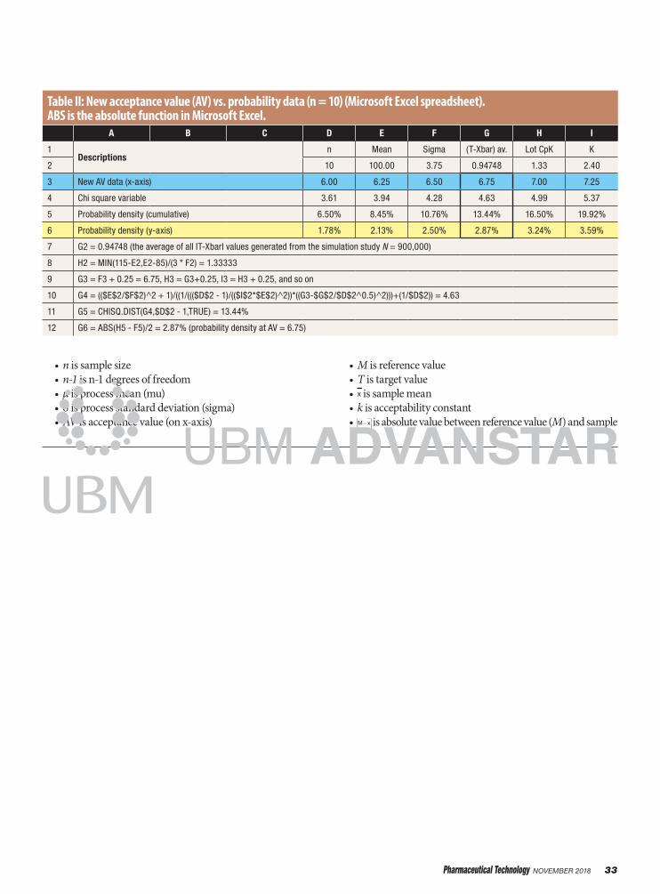
Figure 3: New acceptance value (AV) distributions: Lot Mean and Target = 105% LC (n = 10).

Figure 2: New acceptance value (AV) distributions: Lot Mean and Target = 100% LC (n = 10).

Table III: Microsoft Excel spreadsheet for normal data simulation and acceptance value (AV) calculation. ABS is the absolute function in Microsoft Excel.

A B C D E F G H I

1 Data # Mean 100.00 Sigma 3.75 n 10 k 2.4

2 1 100.76 103.93 103.46 101.53 102.06 98.84 105.63 96.12

3 2 103.19 100.84 97.24 99.83 103.43 102.71 102.77 100.96

… … … … … … … … … …

10 9 103.72 103.77 107.05 96.16 104.06 97.25 95.63 100.59

11 10 102.75 101.24 92.45 95.16 103.77 99.74 101.27 108.42

12 Mean 101.28 100.54 99.61 99.09 101.10 101.72 98.97 100.42

13 SD 2.80 2.87 5.42 3.18 3.10 2.84 4.08 4.62

14 AV 7.13 7.07 13.14 7.92 7.78 7.36 10.13 11.22

15 ABS 1.28 0.54 0.39 0.91 1.10 1.72 1.03 0.42

16 Lot Mean 100.34 Lot SD 3.67 Lot CpK 1.33 ABS avg. 0.92200 N = 90

17 Each simulated normal data cell (B2 through I11) = NORM.INV(RAND(),$C$1,$E$1)

18 B12 = AVERAGE(B2:B11) B16 = AVERAGE(B12:I12) = 100.34

19 B13 = STDEV(B2:B11) D16 = STDEVP(B2:I11) = 3.67

20 B14 =ABS($C$1-B12)/( $G$1^0.5)+$I$1*B13 F16 = MIN(115-B16,B16-85)/(3*D16) = 1.33

21 B15 =ABS($C$1-B12) H16 = AVERAGE(B15:I15) = 0.92200

22 I16 = “N = “&COUNT(B2:I11)&”” = N = 90


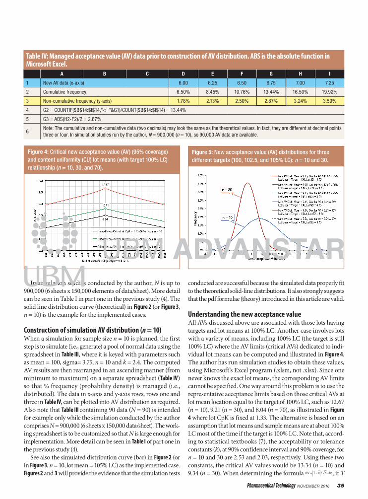
In simulation studies conducted by the author, N is up to 900,000 (6 sheets x 150,000 elements of data/sheet). More detail can be seen in Table I in part one in the previous study (4). The solid line distribution curve (theoretical) in Figure 2 (or Figure 3, n = 10) is the example for the implemented cases.

Construction of simulation AV distribution (n = 10)When a simulation for sample size n = 10 is planned, the first step is to simulate (i.e., generate) a pool of normal data using the spreadsheet in Table III, where it is keyed with parameters such as mean = 100, sigma= 3.75, n = 10 and k = 2.4. The computed AV results are then rearranged in an ascending manner (from minimum to maximum) on a separate spreadsheet (Table IV) so that % frequency (probability density) is managed (i.e., distributed). The data in x-axis and y-axis rows, rows one and three in Table IV, can be plotted into AV distribution as required. Also note that Table III containing 90 data (N = 90) is intended for example only while the simulation conducted by the author comprises N = 900,000 (6 sheets x 150,000 data/sheet). The work-ing spreadsheet is to be customized so that N is large enough for implementation. More detail can be seen in Table I of part one in the previous study (4).

See also the simulated distribution curve (bar) in Figure 2 (or in Figure 3, n = 10, lot mean = 105% LC) as the implemented case. Figures 2 and 3 will provide the evidence that the simulation tests

conducted are successful because the simulated data properly fit to the theoretical solid-line distributions. It also strongly suggests that the pdf formulae (theory) introduced in this article are valid.

Understanding the new acceptance valueAll AVs discussed above are associated with those lots having targets and lot means at 100% LC. Another case involves lots with a variety of means, including 100% LC (the target is still 100% LC) where the AV limits (critical AVs) dedicated to indi-vidual lot means can be computed and illustrated in Figure 4. The author has run simulation studies to obtain these values, using Microsoft’s Excel program (.xlsm, not .xlsx). Since one never knows the exact lot means, the corresponding AV limits cannot be specified. One way around this problem is to use the representative acceptance limits based on those critical AVs at lot mean location equal to the target of 100% LC, such as 12.67 (n = 10), 9.21 (n = 30), and 8.04 (n = 70), as illustrated in Figure 4 where lot CpK is fixed at 1.33. The alternative is based on an assumption that lot means and sample means are at about 100% LC most of the time if the target is 100% LC. Note that, accord-ing to statistical textbooks (7), the acceptability or tolerance constants (k), at 90% confidence interval and 90% coverage, for n = 10 and 30 are 2.53 and 2.03, respectively. Using these two constants, the critical AV values would be 13.34 (n = 10) and 9.34 (n = 30). When determining the formula AV = T x / n +ks, if T

Table IV: Managed acceptance value (AV) data prior to construction of AV distribution. ABS is the absolute function in Microsoft Excel.

A B C D E F G H I

1 New AV data (x-axis) 6.00 6.25 6.50 6.75 7.00 7.25

2 Cumulative frequency 6.50% 8.45% 10.76% 13.44% 16.50% 19.92%

3 Non-cumulative frequency (y-axis) 1.78% 2.13% 2.50% 2.87% 3.24% 3.59%

4 G2 = COUNTIF($B$14:$I$14,"<="&G1)/COUNT($B$14:$I$14) = 13.44%

5 G3 = ABS(H2-F2)/2 = 2.87%

6Note: The cumulative and non-cumulative data (two decimals) may look the same as the theoretical values. In fact, they are different at decimal points three or four. In simulation studies run by the author, N = 900,000 (n = 10), so 90,000 AV data are available.

Figure 4: Critical new acceptance value (AV) (95% coverage) and content uniformity (CU) lot means (with target 100% LC) relationship (n = 10, 30, and 70).

Figure 5: New acceptance value (AV) distributions for three different targets (100, 102.5, and 105% LC): n = 10 and 30.


Peer-Reviewed

increases, x will increase accordingly, so the absolute value will remain nearly the same.

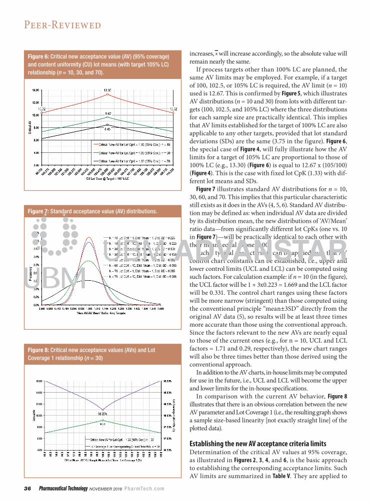
If process targets other than 100% LC are planned, the same AV limits may be employed. For example, if a target of 100, 102.5, or 105% LC is required, the AV limit (n = 10) used is 12.67. This is confirmed by Figure 5, which illustrates AV distributions (n = 10 and 30) from lots with different tar-gets (100, 102.5, and 105% LC) where the three distributions for each sample size are practically identical. This implies that AV limits established for the target of 100% LC are also applicable to any other targets, provided that lot standard deviations (SDs) are the same (3.75 in the figure). Figure 6, the special case of Figure 4, will fully illustrate how the AV limits for a target of 105% LC are proportional to those of 100% LC (e.g., 13.30) (Figure 6) is equal to 12.67 x (105/100) (Figure 4). This is the case with fixed lot CpK (1.33) with dif-ferent lot means and SDs.

Figure 7 illustrates standard AV distributions for n = 10, 30, 60, and 70. This implies that this particular characteristic still exists as it does in the AVs (4, 5, 6). Standard AV distribu-tion may be defined as: when individual AV data are divided by its distribution mean, the new distributions of ‘AV/Mean’ ratio data—from significantly different lot CpKs (one vs. 10 in Figure 7)—will be practically identical to each other with their means equal to one (1.00).

Such a typical characteristic can be applied such that AV control chart constants can be established, i.e., upper and lower control limits (UCL and LCL) can be computed using such factors. For calculation example: if n = 10 (in the figure), the UCL factor will be 1 + 3x0.223 = 1.669 and the LCL factor will be 0.331. The control chart ranges using these factors will be more narrow (stringent) than those computed using the conventional principle “mean±3SD” directly from the original AV data (5), so results will be at least three times more accurate than those using the conventional approach. Since the factors relevant to the new AVs are nearly equal to those of the current ones (e.g., for n = 10, UCL and LCL factors = 1.71 and 0.29, respectively), the new chart ranges will also be three times better than those derived using the conventional approach.

In addition to the AV charts, in-house limits may be computed for use in the future, i.e., UCL and LCL will become the upper and lower limits for the in-house specifications.

In comparison with the current AV behavior, Figure 8 illustrates that there is an obvious correlation between the new AV parameter and Lot Coverage 1 (i.e., the resulting graph shows a sample size-based linearity [not exactly straight line] of the plotted data).

Establishing the new AV acceptance criteria limitsDetermination of the critical AV values at 95% coverage, as illustrated in Figures 2, 3, 4, and 6, is the basic approach to establishing the corresponding acceptance limits. Such AV limits are summarized in Table V. They are applied to

Figure 6: Critical new acceptance value (AV) (95% coverage) and content uniformity (CU) lot means (with target 105% LC) relationship (n = 10, 30, and 70).

Figure 7: Standard acceptance value (AV) distributions.

Figure 8: Critical new acceptance values (AVs) and Lot Coverage 1 relationship (n = 30)


all processes with targets not less than 100% LC. AV and AV average limits must be computed following the calcula-tion examples in Table V. AV average limit requirements are implemented when several batches produced are evaluated (e.g., in continued process verification or process valida-tion batches). The successful average results show that Lot CpK is, on average, not less than 1.33. Table VI introduces the two-stage acceptance criteria for UDU using the new AV limits.

DiscussionJustification of sample mean (x) values is important and assumes that the natural ranges for the mean data are known. In theory, for sample size n the acceptance range is 15∕√n . However, the working ranges about the target must account for some process errors. For example, suppose that the following justification cri-teria are given:

• Individual range: ±15% about the lot mean (justification: “15” is commonly used, i.e., derived from 115% - 100% or 100% - 85% [- is minus]).

• Sample mean range: ±15∕√n% about the lot mean (justifica-tion: this criterion is in the same manner as standard error of the mean σ∕√n).

• Lot mean range (process error): ±1.25% about the target (justification: process error may be not more than 10% of the individual range 15, 1.25% or 8.33% of 15 is determined adequate).

The working mean range will, therefore, be not more than ±(15 / n +1.25) about the target, i.e., T x (15 / n +1.25). In summary using this particular expression, the CU working mean ranges for n = 10, 30, 60, 70, and 140 will be ±6, ±4, ±3.2, ±3, and ±2.5% about the target, respectively, where the target may be 100%, 102.5%, 105% LC or other. See also the calculation examples re-garding “T-Xbar” in Table VII.

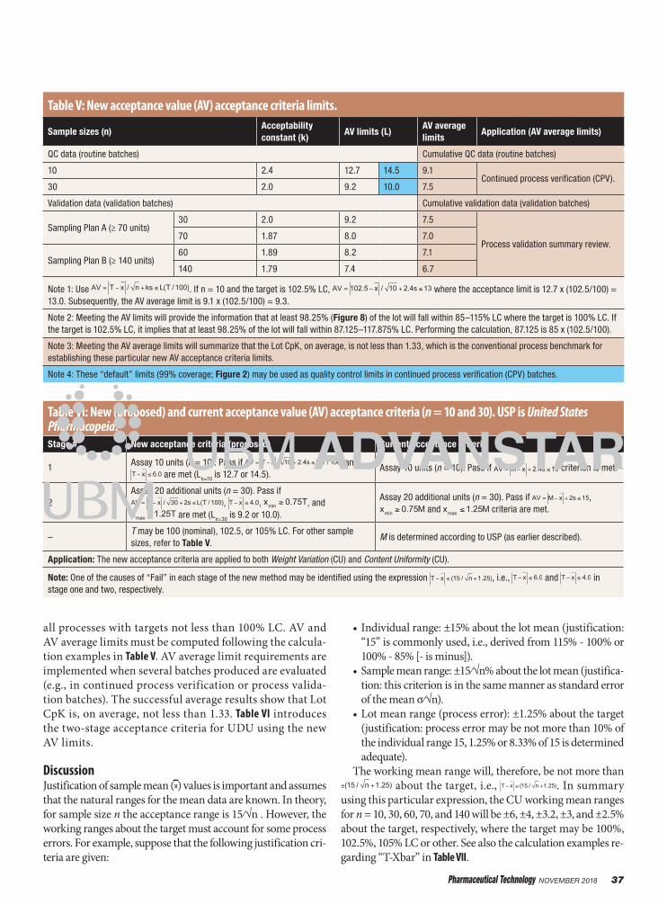
Table V: New acceptance value (AV) acceptance criteria limits.

Sample sizes (n)Acceptability constant (k)

AV limits (L)AV average limits

Application (AV average limits)

QC data (routine batches) Cumulative QC data (routine batches)

10 2.4 12.7 14.5 9.1Continued process verification (CPV).

30 2.0 9.2 10.0 7.5

Validation data (validation batches) Cumulative validation data (validation batches)

Sampling Plan A (≥ 70 units)30 2.0 9.2 7.5

Process validation summary review.70 1.87 8.0 7.0

Sampling Plan B (≥ 140 units)60 1.89 8.2 7.1

140 1.79 7.4 6.7

Note 1: Use AV = T x / n +ks L(T /100). If n = 10 and the target is 102.5% LC, AV = 102.5 x / 10 + 2.4s 13 where the acceptance limit is 12.7 x (102.5/100) = 13.0. Subsequently, the AV average limit is 9.1 x (102.5/100) = 9.3.

Note 2: Meeting the AV limits will provide the information that at least 98.25% (Figure 8) of the lot will fall within 85–115% LC where the target is 100% LC. If the target is 102.5% LC, it implies that at least 98.25% of the lot will fall within 87.125–117.875% LC. Performing the calculation, 87.125 is 85 x (102.5/100).

Note 3: Meeting the AV average limits will summarize that the Lot CpK, on average, is not less than 1.33, which is the conventional process benchmark for establishing these particular new AV acceptance criteria limits.

Note 4: These “default” limits (99% coverage; Figure 2) may be used as quality control limits in continued process verification (CPV) batches.

Table VI: New (proposed) and current acceptance value (AV) acceptance criteria (n = 10 and 30). USP is United States Pharmacopeia.Stage # New acceptance criteria (proposed) Current acceptance criteria

1 Assay 10 units (n = 10). Pass if AV = T x / 10 + 2.4s L(T /100) and T x 6.0 are met (Ln=10 is 12.7 or 14.5).

Assay 10 units (n = 10). Pass if AV = M x + 2.4s 15 criterion is met.

2Assay 20 additional units (n = 30). Pass if AV = T x / 30 + 2s L(T /100), T x 4.0, xmin 0.75T, and xmax 1.25T are met (Ln=30 is 9.2 or 10.0).

Assay 20 additional units (n = 30). Pass if AV = M x + 2s 15, xmin 0.75M and xmax 1.25M criteria are met.

–T may be 100 (nominal), 102.5, or 105% LC. For other sample sizes, refer to Table V.

M is determined according to USP (as earlier described).

Application: The new acceptance criteria are applied to both Weight Variation (CU) and Content Uniformity (CU).

Note: One of the causes of “Fail” in each stage of the new method may be identified using the expression T x (15 / n +1.25), i.e., T x 6.0 and T x 4.0 in stage one and two, respectively.


Using an acceptance threshold of 95 or 99% coverage point is statistically justified. The higher coverage value, at 99% ap-pears to be more practical, however. Such default limits (99%), i.e., 14.5 (n = 10) and 10.0 (n = 30), can be used as quality con-trol (QC) limits in initial batches such as continued process verification (CPV) batches. In routine batches (after successful CPV batches), the 95% coverage working limits, i.e., 12.7 (n = 10) and 9.2 (n = 30), can be used.

After using either default limits (99%) or working limits (95%), the cumulative AV data must be evaluated and included in the annual product review (APR), and, in the future, may be com-puted for use as in-house limits (for quality assurance) in place of the two limits.

Note: The terms “default limit,” “QC limit,” or “working limit” are used in this study, rather than using the terms “official limit” or “specification limit,” because this new AV concept has not yet been recognized by pharmacopeia.

Calculation examplesUsing the data from the calculation examples provided on the USP web page (USP–NF General Chapter <905> “Uniformity of Dosage Units”) (1), the new and current methods are com-pared in Table VII. Note that the new method is more discrimi-native as demonstrated in example two, where the “T-Xbar” data also exceed the acceptance ranges (±6 and ±4 for n = 10 and 30 respectively). In the table, the working formulae are AV = T x / 10 + 2.4s 12.7(T /100) and AV = T x / 30 + 2s 9.2(T /100).

If default limits are employed in the table, the results will be the same (e.g., failure results in example two). This implies that the discriminative power of the 99% coverage limits is also attainable.

Another case involves actual lots of 50-mg tolperisone tablets, where the CU average and SD data are 93.11% and 3.68% LC, respectively (n = 10, target = 100% LC). The computed current and new AVs are 14.22 (not more than 15, i.e., pass) and 11.01 (not more than 12.7), respectively. Although the product passes

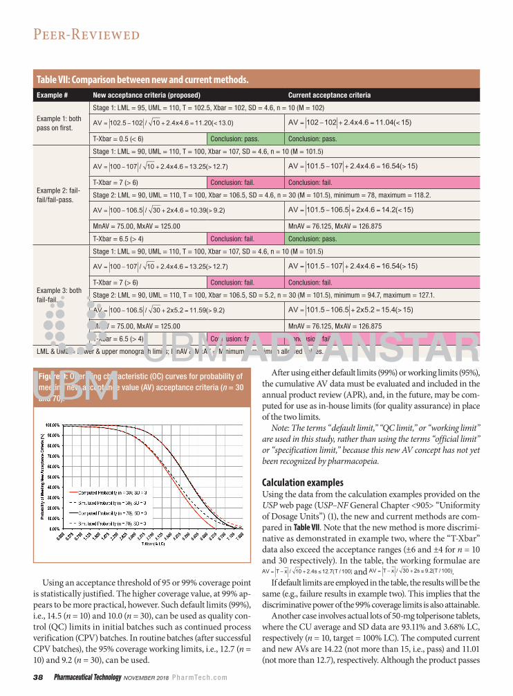
Table VII: Comparison between new and current methods.Example # New acceptance criteria (proposed) Current acceptance criteria

Example 1: both pass on first.

Stage 1: LML = 95, UML = 110, T = 102.5, Xbar = 102, SD = 4.6, n = 10 (M = 102)

AV = 102.5 102 / 10 + 2.4x4.6 =11.20(<13.0) AV = 102 102 + 2.4x4.6 =11.04(<15)

T-Xbar = 0.5 (< 6) Conclusion: pass. Conclusion: pass.

Example 2: fail-fail/fail-pass.

Stage 1: LML = 90, UML = 110, T = 100, Xbar = 107, SD = 4.6, n = 10 (M = 101.5)

AV = 100 107 / 10 + 2.4x4.6 =13.25(>12.7) AV = 101.5 107 + 2.4x4.6 =16.54(>15)

T-Xbar = 7 (> 6) Conclusion: fail. Conclusion: fail.

Stage 2: LML = 90, UML = 110, T = 100, Xbar = 106.5, SD = 4.6, n = 30 (M = 101.5), minimum = 78, maximum = 118.2.

AV = 100 106.5 / 30 + 2x4.6 =10.39(> 9.2) AV = 101.5 106.5 + 2x4.6 =14.2(<15)

MnAV = 75.00, MxAV = 125.00 MnAV = 76.125, MxAV = 126.875

T-Xbar = 6.5 (> 4) Conclusion: fail. Conclusion: pass.

Example 3: both fail-fail.

Stage 1: LML = 90, UML = 110, T = 100, Xbar = 107, SD = 4.6, n = 10 (M = 101.5)

AV = 100 107 / 10 + 2.4x4.6 =13.25(>12.7) AV = 101.5 107 + 2.4x4.6 =16.54(>15)

T-Xbar = 7 (> 6) Conclusion: fail. Conclusion: fail.

Stage 2: LML = 90, UML = 110, T = 100, Xbar = 106.5, SD = 5.2, n = 30 (M = 101.5), minimum = 94.7, maximum = 127.1.

AV = 100 106.5 / 30 + 2x5.2 =11.59(> 9.2) AV = 101.5 106.5 + 2x5.2 =15.4(>15)

MnAV = 75.00, MxAV = 125.00 MnAV = 76.125, MxAV = 126.875

T-Xbar = 6.5 (> 4) Conclusion: fail. Conclusion: fail.

LML & UML = Lower & upper monograph limits; MnAV & MxAV = Minimum & maximum allowed values.

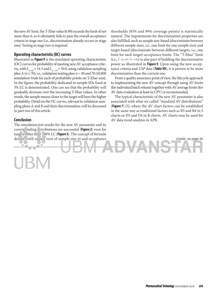
Figure 9: Operating characteristic (OC) curves for probability of meeting new acceptance value (AV) acceptance criteria (n = 30 and 70).

Peer-Reviewed


the new AV limit, the T-Xbar value (6.89) exceeds the limit of not more than 6, so it ultimately fails to pass the overall acceptance criteria in stage one (i.e., discrimination already occurs in stage one). Testing in stage two is required.

Operating characteristic (OC) curvesIllustrated in Figure 9 is the simulated operating characteristic (OC) curves for probability of meeting new AV acceptance crite-ria, with Ln=10 = 14.5 and Ln = 30 = 10.0, using validation sampling plan A (n ≥ 70), i.e., validation testing plan n = 30 and 70 (10,000 simulation trials for each of probability points on T-Xbar axis). In the figure, the probability dedicated to sample SDs fixed at 3% LC is demonstrated. One can see that the probability will gradually decrease over the increasing T-Xbar values. In other words, the sample means closer to the target will have the higher probability. Detail on the OC curves, relevant to validation sam-pling plans A and B and their discrimination, will be discussed in part two of this article.

ConclusionThe simulation test results for the new AV parameter and its corresponding distributions are successful (Figure 2) even for targets other than 100% LC (Figure 3). The concept of formula design (with square root of sample size n) and acceptance

thresholds (95% and 99% coverage points) is statistically natural. The requirements for discrimination properties are also fulfilled, such as sample size-based (discriminate between different sample sizes, i.e., one limit for one sample size) and target-based (discriminate between different targets, i.e., one limit for each target) acceptance limits. The “T-Xbar” limit (i.e., T x (15 / n +1.25)) is also part of building the discriminative power as illustrated in Figure 9. Upon using the new accep-tance criteria and USP data (Table VII), it is proven to be more discriminative than the current one.

From a quality assurance point of view, the lifecycle approach to implementing the new AV concept through using AV limits (for individual batch release) together with AV average limits (for AV data evaluation at least in CPV) is recommended.

The typical characteristic of the new AV parameter is also associated with what we called “standard AV distributions” (Figure 7) (5), where the AV chart factors can be established in the same way as traditional factors such as B3 and B4 in S charts or D3 and D4 in R charts. AV charts may be used for AV data trend analysis in APR.

Contin. on page 45


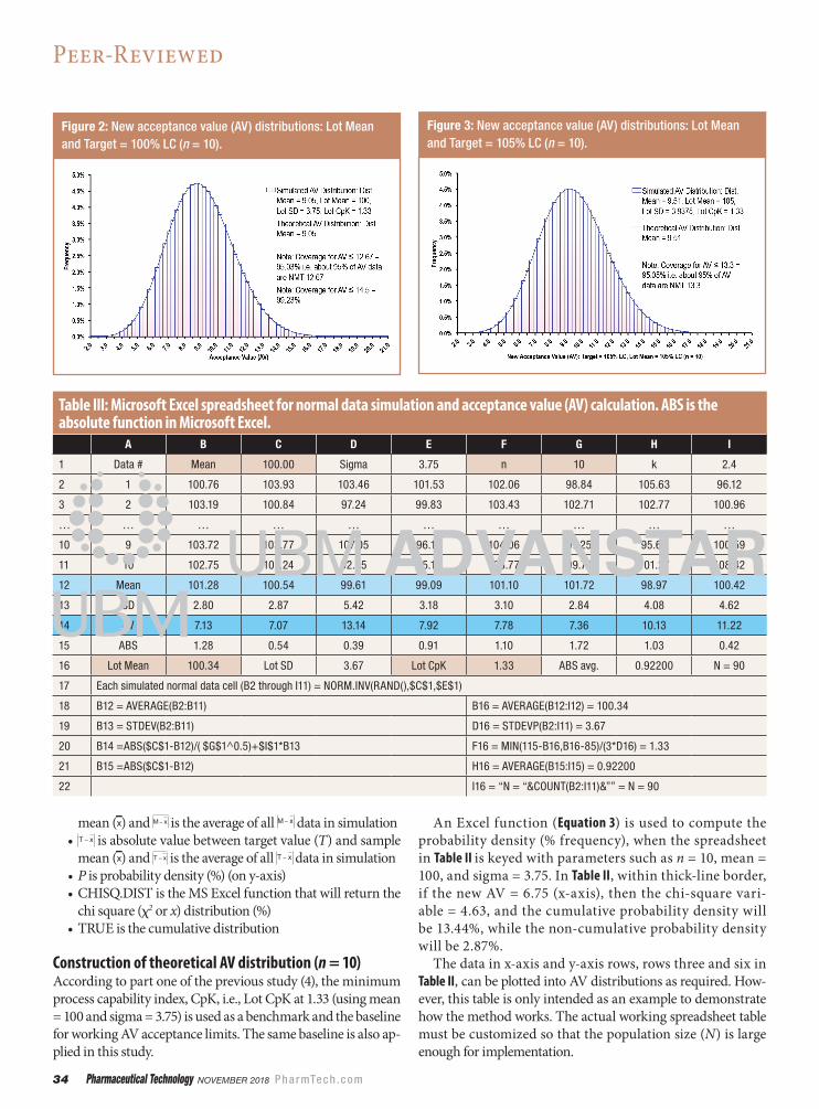
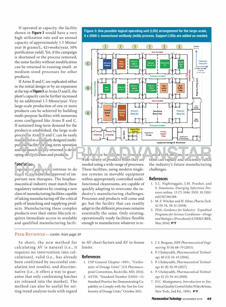
If operated at capacity, the facility shown in Figure 3 would have a very high utilization rate and an annual capacity of approximately 1.5 Mtons/year (6 grams/L, 42+weeks/year, 50% purification yield). Yet, if the campaign is shortened or the process removed, the same facility without modification can be returned to running small- or medium-sized processes for other products.

If Arms B and C are replicated either in the initial design or by an expansion at the top of Figure 3 as Arms D and E, the plant’s capacity can be further increased by an additional 1.5 Mtons/year. Very large-scale production of one or more products can be achieved by building multi-purpose facilities with numerous arms configured like Arms B and C. If sustained long term demand for the product is established, the large-scale process in Arms B and C can be easily transferred to a similarly designed multi-purpose facility for long-term operation and the launch facility returned to devel-oping new processes and products.

ConclusionRegulatory agencies continue to do much to expedite the approval of im-portant new therapies. The biophar-maceutical industry must match these regulatory initiatives by creating a new class of manufacturing facilities capable of taking manufacturing off the critical path of launching and supplying prod-ucts. Manufacturing these complex products over their entire lifecycle re-quires immediate access to available and qualified manufacturing facili-

ties that can be adapted to produce a wide variety of products when they are needed using a wide range of processes. These facilities, using modern single-use systems in movable equipment within appropriately controlled multi-functional cleanrooms, are capable of quickly adapting to overcome the in-dustry’s manufacturing challenges. Processes and products will come and go, but the facility that can readily adapt to the different processes remains essentially the same. Only existing, operationally ready facilities f lexible enough to manufacture whatever is re-

quired with minimal or no modifica-tions can rapidly and efficiently fulfill the industry’s future manufacturing challenges.

References 1. S.L. Nightinggale, J.M. Prasher, and

S. Simonson, Emerging Infectious Dis-eases online, 13 (7) 1046. DOI: 10.3201/eid1307.061188.

2. M. F. Witcher and H. Silver, Pharm.Tech. 42 (9) 34, 38-41 (2018).

3. FDA, Guidance for Industry: Expedited Programs for Serious Conditions—Drugs and Biologics (Procedural) (CDER/CBER, May 2014). PT

Figure 3: One possible logical operating unit (LOU) arrangement for the large-scale, 6 x 2000-L monoclonal antibody (mAb) process. Support LOUs are added as needed.

In shor t , t he new met hod for ca lculating AV is natural (i.e., it requires no intervention into cal-culations), valid (i.e., has already been confirmed by successful sim-ulation test results), and discrimi-native (i.e., it offers a way to guar-antee that only conforming batches are released into the market). The method can also be useful for set-ting trend analysis tools with regard

to AV chart factors and AV in-house limits.

References 1. USP General Chapter <905>, “Unifor-

mity of Dosage Units” (US Pharmaco-peial Convention, Rockville, MD, 2014).

2. ASTM, “Standard Number E2810—11: Standard Practice for Demonstrating Ca-pability to Comply with the Test for Uni-formity of Dosage Units,” October 2011.

3. J. S. Bergum, ISPE Pharmaceutical Engi-neering 35 (6) 68–79 (2015).

4. P. Cholayudth, Pharmaceutical Technol-ogy 40 (12) 34-43 (2016).



7. D.C. Montgomery, Introduction to Sta-tistical Quality Control (John Wiley & Sons, New York, 2nd Ed., 1991). PT

Peer-Reviewed — contin. from page 39

Documents

Uniformity of Dosage Units, Part 1: Acceptance Valuefiles.pharmtech.com/alfresco_images/pharma/2018/11/... · Table I: Current vs. new acceptance value (AV) formulas and how they’re