Embed Size (px)
Citation preview

1
Unified Modeling of Corporate Debt,
Credit Derivatives, and Equity Derivatives*
Vadim Linetsky
Northwestern University [email protected]
http://users.iems.northwestern.edu/~linetsky
FDIC CFR Fellows Workshop October 25-27, Arlington, VA
* Research supported by FDIC, Moody�s, and NSF.

2
Introduction
• In the Black-Scholes-Merton model, the stock price follows geometric
Brownian motion, a process with infinite lifetime (no possibility of
bankruptcy).
• Real-world firms have positive probability of bankruptcy in finite time.
• While many popular stock options pricing models (local vol, stochastic
vol, jump-diffusion, Levy,�) focus on modeling volatility skew and
ignore the possibility of default of the firm underlying the option contract,
modeling default is central to the area of credit risk, corporate debt and
credit derivatives modeling.

3
Motivating Example
Data: General Motors price on 02.22.2006 was $21.19
Historical Volatility of GM stock price over the previous 12 months ~46%
Question: Which exchange-traded option contract (strike and expiration)
on GM had the largest Open Interest? Can you guess its Implied Volatility?

4
Motivating Example
Answer:
• Largest OI: Jan 07 $10 Put @ $1.50 (IV ~100%) with OI 493,051
contracts.
• 2nd largest OI: Jan 07 $5 Put @ $0.50 (IV ~120%) with OI 205,703
contracts.
• Jan 07 $7.50 @ $1.00 (IV ~110%) and $2.50 @ $0.15 (IV ~133%)
Puts also have substantial OI.
• Total outstanding notional for Jan 07 Puts with strikes $2.50-$10
~100 million shares (+ Jan 08 Puts with strikes $2.50-$10 ~30
million shares).

5
Implied Volatility Skew for GM 2007 Puts
40
50
60
70
80
90
100
110
120
130
140
0 5 10 15 20 25 30
Strike Price
Impl
ied
Vola
tility
, %
Recall that 12-month Historical Volatility of GM ~46%!

6
Stock Options as Credit Derivatives
• Put options on the stock provide default protection and can be used to
manage default risk close link between equity and credit derivatives.
• Deep out-of-the-money puts are essentially credit derivatives.
• A rough calculation for Jan 08 $2.50 put. If GM does not go bankrupt, the
put expires worthless. If GM goes bankrupt, GM stock will be worth
pennies. Assume zero. Then the put pays $2.50. Like CDS!
• Price = (discount factor) x (R.N. probability of GM bankruptcy) x $2.50
• Price on 02.22.06 = $0.50, so market implied
Implied R.N. Probability of GM Bankruptcy by Jan 2008 = 22%

7
Further Observations
• On the flip side, pricing and risk management of equity derivatives should
take into account the possibility of default.
• Possibility of default contributes to the implied volatility skew in stock
options. Linkage between implied volatility skew in options markets and
credit spreads in credit markets.
• Corporate debt, credit derivatives, and equity derivatives should be
modeled within a unified framework.

8
Research Program
• We develop a parsimonious, analytically tractable unified modeling
framework for corporate debt, credit derivatives, and equity derivatives.
• In the reduced-form, intensity-based framework, we model Defaultable
Stock as the fundamental state variable.
• We view corporate debt, equity derivatives, and credit derivatives as
contingent claims written on the defaultable stock.
• Our Research Program: introduce default into all the major equity
derivatives models, preserving analytical tractability as much as possible.

9
A Catalogue of Models
I. Jump-to-Default Extended Diffusion (JDD)
I.1 Jump-to-Default Extended Black-Scholes-Merton (JDBSM)
I.2 JDBSM --- 2nd Model Specification
I.3 Jump-to-Default Extended CEV (JDCEV)
II. Stochastic Volatility (SV) Models with Default
II.1 Affine SV Model with Default: Application to Convertible Bonds
II.2 Non-affine Local-Stochastic Volatility Models with Default
III. Models with Jumps
III.1 Introducing Jumps into JDD by Subordination
III.2 Models with Jumps, Stochastic Volatility, and Default

I. Jump-to-Default Extended Diffusion (JDD)
� Model the pre-default stock dynamics under an EMM Q as a diffusion:
dSt = [r(t)− q(t) + λ(St, t)]St dt+ σ(St, t)St dBt, S0 = S > 0,r, q, σ and λ are the short rate, dividend yield, volatility, and default intensity.
� If the diffusion can hit zero, we kill it at the Þrst hitting time of zero, T0, andsend it to a cemetery (bankruptcy) state ∆, where it remains forever.
� Jump-to-default arrives at the Þrst jump time �ζ of a doubly-stochastic Poissonprocess with intensity λ(St, t). The time of default is ζ = min{T0, �ζ}.
� Assume stock holders do not receive any recovery in the event of default. Ad-dition of λ in the drift r − q + λ compensates for default to insure that thediscounted gain process to the stock holders is a martingale under the EMM.
10

Pricing Corporate Bonds
� The time-t price of a defaultable zero-coupon bond with face value of $1and no recovery in default:
B(S, t;T ) = e−R Ttr(u)duQ(S, t;T ),
where the (risk-neutral) survival probability is:
Q(S, t;T ) = E[e−R Ttλ(Su,u)du1{T0>T}|St = S].
11
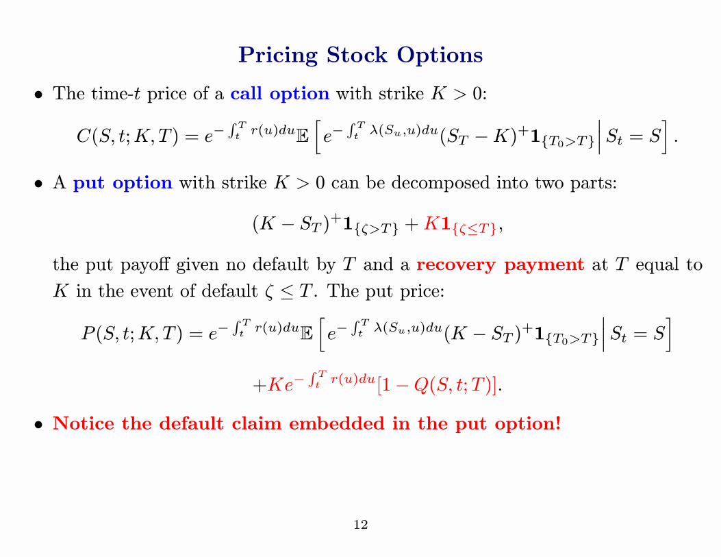
Pricing Stock Options
� The time-t price of a call option with strike K > 0:
C(S, t;K,T ) = e−R Ttr(u)duE
he−
R Ttλ(Su,u)du(ST −K)+1{T0>T}
¯St = S
i.
� A put option with strike K > 0 can be decomposed into two parts:
(K − ST )+1{ζ>T} +K1{ζ≤T},the put payoff given no default by T and a recovery payment at T equal to
K in the event of default ζ ≤ T . The put price:
P (S, t;K,T ) = e−R Ttr(u)duE
he−
R Ttλ(Su,u)du(K − ST )+1{T0>T}
¯St = S
i+Ke−
R Ttr(u)du[1−Q(S, t;T )].
� Notice the default claim embedded in the put option!
12

I.1 A Jump-to-Default Extended Black-Scholes-Merton
� Pre-default stock price dynamics:dSt = [r − q + λ(St)]St dt+ σSt dBt, S0 = S > 0,
λ(S) =α
Sp, α > 0, p > 0.
� This process cannot diffuse to zero. Time of default ζ is the Þrst jump timeof a doubly stochastic Poisson process with intensity λ(S).
� λ(S)→∞ as S → 0, making default inevitable at low stock prices.
� λ(S)→ 0 as S →∞, making the stock asymptotically GBM at large values.
� We obtain closed-form solutions in this model (V.L., �Pricing Equity
Derivatives subject to Bankruptcy,� Mathematical Finance, 2006, 16
(2), 255-282.
13
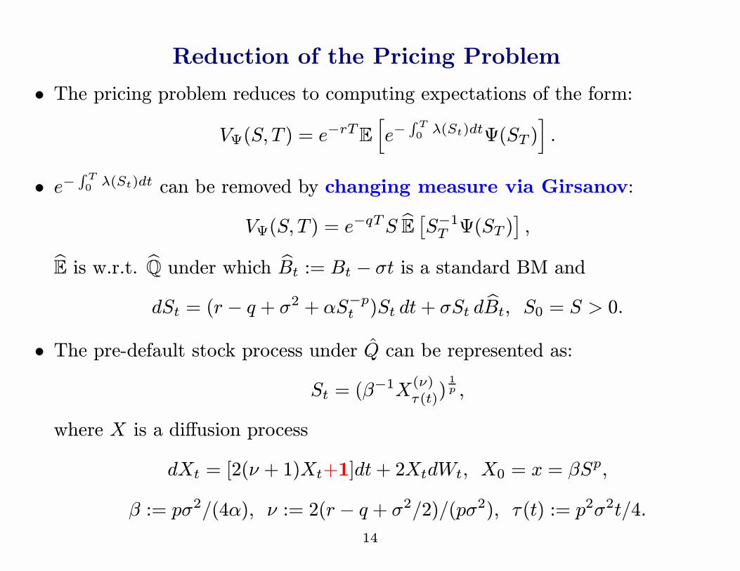
Reduction of the Pricing Problem
� The pricing problem reduces to computing expectations of the form:
VΨ(S, T ) = e−rTE
he−
RT0λ(St)dtΨ(ST )
i.
� e−R T0λ(St)dt can be removed by changing measure via Girsanov:
VΨ(S, T ) = e−qTS bE £S−1T Ψ(ST )
¤,bE is w.r.t. bQ under which bBt := Bt − σt is a standard BM and
dSt = (r − q + σ2 + αS−pt )St dt+ σSt d bBt, S0 = S > 0.� The pre-default stock process under �Q can be represented as:
St = (β−1X(ν)
τ(t))1p ,
where X is a diffusion process
dXt = [2(ν + 1)Xt+1]dt+ 2XtdWt, X0 = x = βSp,
β := pσ2/(4α), ν := 2(r − q + σ2/2)/(pσ2), τ(t) := p2σ2t/4.14

Reduction of the Pricing Problem
� The problem reduces to computing
VΨ(S, T ) = e−qTSE(ν)x [(Xτ/β)
− 1pΨ((Xτ/β)
1p )],
where E(ν)x is w.r.t. the probability law of X starting at x = βSp.
� The process X is closely related to the problem of pricing Asian options (Ge-
man and Yor (1993), Donati-Martin and Yor (2001), Linetsky (2004)).
� The spectral expansion of the transition density of X is available in closed form,
yielding closed-form pricing formulas for corporate bonds and stock options in
the form of spectral expansions.
15

Closed Form Solution for Corporate Bonds
� Zero-coupon bond with unit face and no recovery:
B(S, 0;T ) = 1{ν>2/p}e−rTΓ(ν − 1/p)Γ(ν − 2/p)U
µ1
p,2
p− ν + 1, 1
2x
¶+1{ν<0}e−qT
Γ(1/p− ν)Γ(−ν) (2x)
1p
+1{ν<−2}e−qT[|ν|/2]Xn=1
e−2n(|ν|−n)τ(|ν|− 2n)Γ(−1/p)Γ(1/p + |ν|− n)Γ(1 + |ν|− n)Γ(1− 1/p− n) (2x)
1p+nL(|ν|−2n)n
µ1
2x
+e−qT
4π2Γ(1/p)
Z ∞
0
e−(ν2+ρ2)τ
2 (2x)1p+
1−ν2 e
14xW1−ν
2 ,iρ2
µ1
2x
¶ ¯Γ
µν + iρ
2
¶Γ
µ1
p− ν + iρ
2
¶¯2sinh(πρ)ρ dρ,
U(a, b, z) � Tricomi conßuent hypergeometric function, Wκ,µ(z) � 2nd Whittaker
function, L(α)n (z) � generalized Laguerre polynomials, Γ(z) �Gamma function, [x]
� integer part of x.
� Continuous spectrum above ν2
2 and discrete eigenvalues in [0,ν2
2 ).
� The formulas are fast and easy to compute in Mathematica and Maplewhere all special functions are available.
16

Closed Form Solution for Put Options
P (S, 0;K,T ) = e−rTK − 1{ν>2/p}e−rTKΓ(ν − 1/p)Γ(ν − 2/p)U
µ1
p,2
p− ν + 1, 1
2x
¶−1{ν<0}e
−qTSΓ(|ν|)
∙Γ
µ|ν|, 1
2k
¶+ (2k)
1pγ
µ1
p+ |ν|, 1
2k
¶¸
−1{ν<−2}e−qTS[|ν|/2]Xn=1
pK(n)e−2n(|ν|−n)τ 2(|ν|− 2n)n!
Γ(1 + |ν|− n)(2x)nL(|ν|−2n)n
µ1
2x
−e−qTS 1
2π2
Z ∞
0
PK(ρ)e− (ν2+ρ2)τ
2 x1−ν2 e
14xW1−ν
2 ,iρ2
µ1
2x
¶ ¯Γ
µν + iρ
2
¶¯2sinh(πρ)ρdρ,
where
PK(ρ) = k1+ν2 e−
14kW− 1+ν
2 ,iρ2
µ1
2k
¶+2<
((2k)
ν−iρ2 (2/p− ν − iρ)Γ (−iρ)
Γ(ν/2− iρ/2)(ρ2 + (ν − 2/p)2) 2F2
∙1
p− ν2+iρ
2, 1− ν
2+iρ
2; 1 + iρ,
1
p− ν2+iρ
2+ 1;− 1
2k
¸¾,
pK(n) = − 1
2n(2k)n−|ν|e−
12kL
(|ν|−2n)n−1
µ1
2k
¶+
Γ(|ν|− n+ 1)(2k)n−|ν|2(|ν|− n+ 1/p)n!Γ(|ν|− 2n+ 1) 2F2
∙|ν|− n+ 1, |ν|− n+ 1
p; |ν|− 2n+ 1, |ν|− n+ 1 + 1
p;− 12k
¸,
2F2[a1, a2; b1, b2; z] �Gauss hypergeometric function, γ(a, z) � incomplete Gamma
function, Γ(a, z) � complementary incomplete Gamma function, <(z) � real part
of a complex number z.
17

������������������� �������� ��
�
���
���
���
���
�
���
���
���
���
�
� � �� �� �� �� �� �� �� �� ��
����������������������
��� �������� ���
� ���
� �
� �
� �
Figure 1: Term Structure of Credit Spreads. Parameter values: S = S∗ = 50,σ = 0.3, r = q = 0.03, h∗ = 0.03, p = 0.5, 1, 2, 3. λ(S) = h∗
¡S∗S
¢p, where S∗ > 0 is
some reference price level and h∗ = λ(S∗) > 0 (h∗ is the scale parameter).18

!��"�� �#"���"����
��
��
��
��
��
��
��
��
��
$�
$�
��
�� �� �� �� �� �� �� �� ��
����%�
!��"�� �#"���"������
� ����
� ���
� �
� �
Figure 2: Implied Volatilities for Times to Expiration T = 0.25, 0.5, 1, 5.Parameter values: S = S∗ = 50, σ = 0.3, r = q = 0.03, h∗ = 0.03, p = 2 (the sameparameters used to compute credit spreads).
19

I.2 Alternative Intensity SpeciÞcation
� Alternative intensity speciÞcation:
λ(S) =c
ln(S/B), c > 0, B > 0, S > B.
This speciÞcation is similar to the one used in Madan and Unal (1998).
� λ(S) → ∞ as S → B, making default inevitable as the stock falls towards B.
λ(S)→ 0 as S →∞.� The pricing problem reduces to computing expectations of the form:
VΨ(S, T ) = e−rTE
he−
R T0λ(St)dtΨ(ST )
i= e−qTS bE £S−1T Ψ(ST )
¤,
bE is w.r.t. bQ under which bBt := Bt − σt is a standard BM and
dSt = (r − q + σ2 + c/ ln(St/B))St dt+ σSt d bBt, S0 = S > B.� We obtain closed-form solutions in this model.
20

Reduction to Bessel Process with Drift
� Let X be a Bessel process with drift:
dXt =
µν + 1/2
Xt+ µ
¶dt+ dWt, X0 = x > 0.
� The pre-default stock process under �Q can be represented as:St = Be
σXt where ν = c/σ2 − 1/2, µ = (r − q)/σ + σ/2, x = ln(S/B)/σ.
� The problem reduces to computing
VΨ(S, T ) = e−qT (S/B)E(ν,µ)x [e−σXTΨ(BeσXT )],
where E(ν,µ)x is w.r.t. the probability law of X starting at x = ln(S/B)/σ.
� Laplace transform of transition density of X was obtained by Yor (1984). It
was inverted by V. Linetsky, �The Spectral Representation of Bessel Processes
with Drift,� J. Appl. Probability, 41 (2004) 327-344. This yields an analytical
solution to our model (in preparation).
21
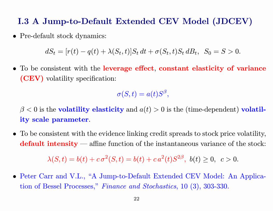
I.3 A Jump-to-Default Extended CEV Model (JDCEV)
� Pre-default stock dynamics:dSt = [r(t)− q(t) + λ(St, t)]St dt+ σ(St, t)St dBt, S0 = S > 0.
� To be consistent with the leverage effect, constant elasticity of variance(CEV) volatility speciÞcation:
σ(S, t) = a(t)Sβ ,
β < 0 is the volatility elasticity and a(t) > 0 is the (time-dependent) volatil-
ity scale parameter.
� To be consistent with the evidence linking credit spreads to stock price volatility,default intensity� affine function of the instantaneous variance of the stock:
λ(S, t) = b(t) + cσ2(S, t) = b(t) + c a2(t)S2β, b(t) ≥ 0, c > 0.
� Peter Carr and V.L., �A Jump-to-Default Extended CEV Model: An Applica-tion of Bessel Processes,� Finance and Stochastics, 10 (3), 303-330.
22

Reduction of JDCEV to CEV
Linetsky & Mendoza recently (two weeks ago) proved that calculations in JDCEV
can be reduced to the standard CEV without jump-to-default by changes of variables
and changes of measure:
VΨ(S, t;T ) = e− R T
tr(u)duEt,S
he−
RTtλ(Su,u)duΨ(ST )1{T0>T}
i= e−
RTt�r(u)dux−
2c2c+1 �Et,x
∙X
2c2c+1
T Ψ(X1
2c+1
T )1{T0>T}
¸,
where x = S1+2c and, under �Q, X follows a standard CEV process:
dXt = [�r(t)− q(t)]Xtdt+ �a(t)X �β+1t d �Bt
with parameters:
�r(t) = (2c+ 1)(r(t) + b(t))− 2cq(t), �a(t) = (2c+ 1)a(t), �β = (2c+ 1)β.
23

Non-central Chi-square Distribution
� CEV transition density is expressed in terms of non-central chi-square.� χ2(δ,α) with δ degrees of freedom and non-centrality parameter α > 0:
fχ2(x; δ,α) =1
2e−
α+x2
³xα
´ ν2
Iν(√xα)1{x>0},
where ν = δ/2− 1 and Iν is the Bessel function.� For p > −(ν + 1) and k > 0, p−th moment and truncated p−th moments:
M(p; δ,α) = Eχ2(δ,α)[Xp] = 2pe−
α2Γ(p+ ν + 1)
Γ(ν + 1)1F1(p+ ν + 1, ν + 1,α/2),
Φ+(p, k; δ,α) = Eχ2(δ,α)[Xp1{X>k}] = 2
p∞Xn=0
e−α2
³α2
´n Γ(ν + p+ n+ 1, k/2)n!Γ(ν + n+ 1)
,
Γ(a) � Gamma function, γ(a, x) � incomplete Gamma function, Γ(a, x) � comple-
mentary incomplete Gamma function, 1F1(a, b, x) � conßuent hypergeometric func-
tion.
24

Results for Survival Probability and Options
� DeÞne x := 1|β|S
|β| > 0, ν+ :=c+1/2|β| > 0, δ+ := 2(ν+ + 1) > 0,
τ = τ(t, T ) :=
Z T
t
a2(u)e−2|β|R utα(s)dsdu.
� Assume no default by time t ≥ 0. The risk-neutral survival probability is:
Q(S, t;T ) = e−RTtb(u)du
µx2
τ
¶ 12|β|
Mµ− 1
2|β| ; δ+,x2
τ
¶.
� The call option price is:
C(S, t;K,T ) = e−RTtq(u)duSΦ+
µ0,k2
τ; δ+,
x2
τ
−e−R Tt[r(u)+b(u)]duK
µx2
τ
¶ 12|β|
Φ+µ− 1
2|β| ,k2
τ; δ+,
x2
τ
¶,
k = k(t, T ) =1
|β|K|β|e−|β|
R Ttα(u)du.
25

Numerical Examples
� Consider a time-homogeneous model.� Parameterize volatility as follows:
σ(S) = σ∗
µS
S∗
¶β,
S∗ > 0 is some reference stock price level and σ∗ > 0 is the volatility at that
reference level, σ(S∗) = σ∗ (e.g., S∗ = S0, initial stock price).
� Assume S0 = 50, σ∗ = 0.2, r = 0.05, q = 0, and the elasticity parameter β = −1.� Default intensity:
λ(S) = b+ cσ2∗
µS
S∗
¶2β.
Consider cases b = 0 and b = 0.02 and c = 1/2 and c = 1.
26

������������������� �������� ��
�����
�����
�����
�����
�����
�����
�����
� � �� �� �� �� �� �� �� �� ��
����������������������
& �
& �� �'�
& �� �
& ����� �'�
& ����� �
Figure 3: Term structures of credit spreads. Parameter values: S0 = 50, σ∗ =0.2, β = −1, r = 0.05, q = 0, b = 0, 0.02, c = 0, 1/2, 1.
27

!��"�� �#"���"�����%�(��
��
��
��
��
��
��
��
��
��
��
��
$�
$�
�� �� �� �� �� �� �� ��
����%�
!��"�� �#"���"������
)*�+#�� ����
)*�+#�� ���
)*�+#�� �
)*�+#�� �
�+#�� ����
�+#�� �
Figure 4: Implied volatility skews. Parameter values: S = S∗ = 50, σ∗ = 0.2, β = −1, r = 0.05,q = 0. For CEV model: b = c = 0. For JDCEV model: b = 0.02, c = 1. JDCEV times to expiration
are T = 0.25, 0.5, 1, 5 years. Implied volatilities are plotted against strike.
28

II.1 Affine Stochastic Volatility Model with Default
� Affine SV model with default and stochastic rates (extenstion of Carr & Wu
(2005) with stochastic rates):
dSt = (rt − q + λt)Stdt+pVtStdW
St ,
drt = κr(θr − rt)dt+ σr√rt dW rt ,
dVt = κV (θV − Vt)dt+ σVpVt dW
Vt ,
dzt = κz(θz + γVt − zt)dt+ σz√zt dW zt ,
λt = zt + αVt + βrt,
dWSt dW
Vt = ρSV dt, ρSV < 0,
other correlations equal to zero.
� The model is affine and analytically tractable for European-style securities, incl.defaultable bonds and stock options, up to Fourier inversion.
29

Figure 5: Implied Vol Skews for T = 0.25, 0.5, 1, and 2 years. Current stock price S0 = 25.
Volatility Skew
Similar to JDCEV, default intensity linearly depends on local vari-ance.
The model features realistic volatility skews linked with credit spreads.
30

Application to Convertible Bonds
� Convertible bonds are American-style. The problem is to Þnd an optimal
conversion strategy for the bondholder and an optimal call strategy for the
Þrm, and value the convertible bond assuming both players behave optimally:
a differential game problem.
� Solving it in the 4-factor model is computationally very challenging!� We convert the differential game to a non-linear penalized PDE and solve itnumerically by the Þnite element method-of-lines with the adaptive time-
stepping package SUNDIALS from the Lawrence Livermore National Labo-
ratory. Kovalov and Linetsky, �Valuing Convertible Bonds with Stock Price,
Volatility, Interest Rate, and Default Risk�, working paper.
31

Figure 6: Solution for the 5-year Convertible Bond (semiannual 3% coupon, 2 years
call protection period, and clean call price $1400). Solid lines � call boundary,
dashed lines � conversion boundary.
32

II.2 Non-affine Local-Stochastic Vol. Models with Default
� Start with a model with local volatility σ(x):dXt = λ(Xt)Xtdt+ σ(Xt)XtdBt
where default arrives with intensity λ(Xt), sending X to zero.
� Suppose Vt follows a CIR process:dVt = κ(θ − Vt)dt+ σV
pVtdWt.
Consider an integral: Tt =R t0Vudu.
� Do a time change St = XTt . The SDE is:dSt = λ(St, Vt)Stdt+ σ(St)
pVtStdBt
and default intensity is λ(S, V ) = λ(S)V .
� If X has an analytically tractable spectral expansion, then S is also tractable
since we know the Laplace transform E[e−sTt ]. We introduce SV into JDD mod-els, and default intensity is linear in stochastic volatility! For the JDCEVSV,
λ(S, V ) = bV + cV a2S2β . Work in progress.
33

Time Changing Diffusions with Known Spectral Expansions
� Transition densities of 1D diffusions admit spectral expansions. If the spectrumof the inÞnitesimal generator of the diffusion X is discrete with eigenvalues λnand eigenfunctions ϕn(x), then the transition density has the spectral expansion:
p(t;x, y) = m(y)∞Xn=1
e−λntϕn(x)ϕn(y),
where m(y) is the speed density of X. If the spectrum is continuous, the sum
is replaced with the integral.
� Suppose Tt is a non-decreasing process with the known Laplace transform:L(t,λ) = E[e−λTt ].
� Then the time-changed process XTt has the transition density:
p(t;x, y) = m(y)∞Xn=1
L(t,λn)ϕn(x)ϕn(y).
� We can construct new tractable processes from a diffusion X with the known
spectral expansion and a time change T with the known Laplace transform.34

III.1 Introducing Jumps by Subordination
� Start with a model with local volatility σ(x) and default intensity λ(x):dXt = λ(Xt)Xtdt+ σ(Xt)XtdBt.
� Suppose {Tt, t ≥ 0} is a Levy subordinator, i.e., a non-decreasing Levy process(only positive jumps). Its Laplace transform is:
E[e−sTt ] = e−tφ(s)
with Laplace exponent φ(s) given by the Levy-Khintcine Theorem.
� Do a time change St = XTt . It is a jump-diffusion process with the same
diffusion volatility as X, with jumps with Levy density and default intensity:
πφ(S, S0) =Z ∞
0
p(t;S, S0)ν(dt), λφ(S) = λ(S) +Z ∞
0
Pd(S, t)ν(dt),
p(t;x, y) � transition density of Xt, Pd(x, t) � probability of default of X by
time t starting from state x at time zero, ν � Levy measure of T .
� S has an analytically tractable spectral expansion if X is, and we have a way of
introducing jumps into our JDD framework. Work in progress with Peter Carr.35

III.2 Models with Jumps, SV, and Default
� If we compose the two types of time changes, then we can build very rich modelswith stochastic volatility, jumps, and default.
� Start with X as before, Þrst do the time change with the Levy subordinator T 1t ,
and then do the time change with T 2t =R t0Vudu. The result is a jump-diffusion
process with jumps, SV, and default with diffusion volatility σ(S, V ) = σ(S)√V ,
Levy measure
πφ(V, S, S0) = VZ ∞
0
p(t;S, S)ν(dt),
and default intensity
λφ(S, V ) = V
∙λ(S) +
Z ∞
0
Pd(S, t)ν(dt)
¸.
� S is analytically tractable if X is, and we have a way of introducing jumps and
SV into our JDD framework. Work in progress with Peter Carr.
36

Conclusion
� We develop a framework for uniÞed modeling of corporate debt, credit deriva-tives, and equity derivatives.
� Within this framework, we are able to go surprisingly far in obtaining analyticalsolutions to credit-equity models with diffusion, jumps, SV, and default.
� Our research program is to introduce default into all the major equity models,
incl. SV, Levy, etc.
� These models feature linkages between corporate credit spreads in the creditmarkets and implied volatility skews in the options markets.
� Equity options may be used as indicators of market�s assessment of credit risk ofthe underlying Þrm along with credit spreads, and are emerging as an important
source of market data to potentially improve credit risk measurement.
37

This talk is based on:
� Linetsky, �Pricing Equity Derivatives subject to Bankruptcy,� MathematicalFinance, 2006, 16 (2), 255-282.
� Carr and Linetsky, �A Jump-to-Default Extended CEV Model: An Applicationof Bessel Processes,� Finance and Stochastics, 10 (3), 303-330.
� Linetsky, �Spectral Methods in Derivatives Pricing,� to appear in Handbook ofFinancial Engineering, Eds. Birge and Linetsky, Elsevier.
� Kovalov and Linetsky, �Valuing Convertible Bonds with Stock Price, Volatility,Interest Rate, and Default Risk,� working paper.
� Linetsky andMendoza, �A Note on the Jump-to-Default Extended CEVModel,�in preparation.
� Linetsky, �UniÞed Valuation of Corporate Debt, Credit Derivatives, and EquityDerivatives,� in progress.
� Carr and Linetsky, �Time Changed Markov Processes in Asset Pricing,� inprogress.
38


![Towards A Unified Theory Of Alkaline Scale Formation From ...€¦ · Synthesis of New Bithiophene and Thieno [2,3-d] Pyrimidine Derivatives with Potent Antimicrobial Activity Hanaa](https://img.pdfslide.us/doc/110x75/5f6cdc2b034a085af149e565/towards-a-unified-theory-of-alkaline-scale-formation-from-synthesis-of-new-bithiophene.jpg)