Intelligent Control and Automation, 2011, 2, 8-23 doi:10.4236/ica.2011.21002 Published Online February 2011 (http://www.SciRP.org/journal/ica)

Copyright © 2011 SciRes. ICA

Unified Modeling Approach of Kinematics, Dynamics and Control of a Free-Flying Space Robot Interacting with a

Target Satellite

Murad Shibli Mechanical Engineering Department, College of Engineering, United Arab Emirates University, Al-Ain, UAE

E-mail: malshibli@uaeu.ac.ae desired Received November 28, 2010; revised December 12, 2010; accepted December 13, 2010

Abstract In this paper a unified control-oriented modeling approach is proposed to deal with the kinematics, linear and angular momentum, contact constraints and dynamics of a free-flying space robot interacting with a target satellite. This developed approach combines the dynamics of both systems in one structure along with holo-nomic and nonholonomic constraints in a single framework. Furthermore, this modeling allows considering the generalized contact forces between the space robot end-effecter and the target satellite as internal forces rather than external forces. As a result of this approach, linear and angular momentum will form holonomic and nonholonomic constraints, respectively. Meanwhile, restricting the motion of the space robot end-effector on the surface of the target satellite will impose geometric constraints. The proposed momentum of the combined system under consideration is a generalization of the momentum model of a free-flying space robot. Based on this unified model, three reduced models are developed. The first reduced dynamics can be considered as a generalization of a free-flying robot without contact with a target satellite. In this re-duced model it is found that the Jacobian and inertia matrices can be considered as an extension of those of a free-flying space robot. Since control of the base attitude rather than its translation is preferred in certain cases, a second reduced model is obtained by eliminating the base linear motion dynamics. For the purpose of the controller development, a third reduced-order dynamical model is then obtained by finding a common solution of all constraints using the concept of orthogonal projection matrices. The objective of this approach is to design a controller to track motion trajectory while regulating the force interaction between the space robot and the target satellite. Many space missions can benefit from such a modeling system, for example, autonomous docking of satellites, rescuing satellites, and satellite servicing, where it is vital to limit the con-tact force during the robotic operation. Moreover, Inverse dynamics and adaptive inverse dynamics control-lers are designed to achieve the control objectives. Both controllers are found to be effective to meet the spe-cifications and to overcome the un-actuation of the target satellite. Finally, simulation is demonstrated by to verify the analytical results. Keywords: Free-Flying Space Robot, Target Satellite, Servicing Flying Robot, Adaptive Control, Inverse

Dynamic Control, Hubble Telescope

1. Introduction Free-flying space robots and free-floating space robots have been under intensive consideration to perform many space missions such as: inspection, maintenance, repair-ing and servicing satellites in earth orbit. Particularly, servicing satellite equipped with robot arms can be em-ployed for recovering the attitude, charging the exhaust-ing batteries, attaching new thrusters, and replacing the

failed parts like gyros, solar panels or antennas of anoth-er satellite.

There are two major classes of space robots can be classified: 1) free-flying space robots and 2) free-floating space robots. The manipulator system of the first type is a system in which the reaction jets (thrusters) are kept active so as to control the position and attitude of the systems’ spacecraft. In opposition to the free flying robot, a free-floating space robotic system is a system in which

M. SHIBLI

Copyright © 2011 SciRes. ICA

9

the spacecrafts’ reaction thrusters are shut down to con-serve attitude control fuel.

Comprehensive understanding of the kinematics and momentum of space robots and their interaction with a floating object is considered as a very essential part in designing an efficient multi-body system with effective control techniques of contact forces and motion trajecto-ries. Many techniques in dynamic modeling of space robots have been developed in [1-10]. Kinematics mo-tion of a space robot system are developed based on the concept of a Virtual Manipulator (VM) [10-14]. It as-sumes imaginary mechanical links and it does not model the angular momentum, then the attitude motion of the base satellite has to be considered by other means. One body of the space robotic system is used as the reference frame with a point on it to represent the transitional DOF of the system [2,8,9]. A tree topology of open chain mul-ti-body system with the system center of mass as the translational DOF is proposed in [6,7].

Many techniques in dynamic modeling of space robots have been reviewed in [2,4,5]. Newton-Euler dynamic approach of multi-body systems is proposed in [6,7]. This approach is characterized the use of a tree topology of open chain multi-body system with the system Center of Mass as the translational DOF. Barycenters are used efficiently to formulate the kinematics and dynamics of free-floating space robots. Another approach is called the direct approach and it uses one body of the system to be the reference frame with a point on it to represent the transitional DOF of the system [2,8,9]. This approach is simpler but results in coupled equations. A virtual mani-pulator is proposed in [10-14] and used to simplify the system dynamics of space robots. It decouples the system Center of Mass transactional DOF.

Free-flying space robots dedicated for maintenance or rescue operations are involved in contact tasks. Many studies on space-based robotic systems have assumed zero external applied forces. Dynamics of space robots by using what is so-called the virtual manipulator (VM) is proposed in [10-14]. Multi-body systems approach based on Newton-Euler dynamic is proposed in [6,7]. Achievements in Space Robotics are presented in [15]. In this article three parts are introduced. In the first part, the achievements of orbital robotics technology in the last decade are reviewed, highlighting the Engineering Test Satellite (ETS-VII) and Orbital Express flight demon-strations. In the second part, some of the selected topics of planetary robotics from the field robotics research point of view are described. Finally, technological chal-lenges to asteroid robotics are discussed.

In work [16] three dynamical models of a two link space robot are developed. One model treats the gravita-tional field as constant over the volume of the robot and

another model uses 0th order Taylor series expansions of a continuous gravitational field over the volume of the robot. A third model neglects the effects of gravity. The dynamics of a dual-arm space robot system was syste-matically studied, and a dynamic model based on Kane-Huston’s method and screw theory was presented in [17]. The numerical example shows that acting mo-ment of a composition unit of the robot can be solved for given value of motion parameters with the exploitation of the dynamic model, vice versa. A simulation system of a three layer structure based on ADAMS, MATLAB and VC++ is present in [18], which can simulate and analyze the kinematics and dynamics of space robot in the process of capturing and releasing space object. Veri-fication results show that this system can well explain space robot’s dynamic and kinetic characteristic in cap-turing and releasing task under the space circumstances.

In research [19], the kinematics and dynamics of free- floating coordinated space robotic system with closed kinematic constraints are developed. An approach to position and force control of free-floating coordinated space robots with closed kinematic constraints is pro-posed for the first time. Unlike previous coordinated space robot control methods which are for open kine-matic chains, the method presented here addresses the main difficult problem of control of closed kinematic chains. The controller consists of two parts, position controller and internal force controller, which regulate, respectively, the object position and internal forces be-tween the object and end-effectors. The inverse kinemat-ic control based on mutual mapping neural network of free-floating dual-arm space robot system without the basepsilas control is discussed in [20]. With the geome-trical relation and the linear, angular momentum conser-vation of the system, the generalized Jacobian matrix is obtained. Based on the above result, a mutual mapping neural network control scheme employing Lyapunov functions is designed to control the end-effectors to track the desired trajectory in workspace. The control scheme does not require the inverse of the Jacobian matrix. A planar dual-arm space robot system is simulated to verify the proposed control scheme. In [21], the kinematics of the FFSR is introduced firstly. Then the null space ap-proach is used to reparameterize the path: the direction and magnitude are decoupled and no direction error is introduced. And the Newton iterative method is adopted to find the optimal magnitude of the joint velocity. A planar FFSR with a 2 DOFs manipulator is selected to test the algorithm and simulation results illustrate that the path following is realized precisely. The genetic algo-rithm with wavelet approximation is applied to nonho-lonomic motion planning in [22-25]. The problem of nonholonomic motion planning is formulated as an op-

M. SHIBLI

Copyright © 2011 SciRes. ICA

10

timal control problem for a drift. The problem of position control of robotic manipula-

tors both nonredundant and redundant in the task space is addressed in [26]. A computationally simple class of task space regulators consisting of a transpose adaptive Jaco-bian controller plus an adaptive term estimating genera-lized gravity forces is proposed. The Lyapunov stability theory is used to derive the control scheme. In [27] glob-al randomized joint-space path planning for articulated robots that are subjected to task-space constraints is ex-plored. This paper describes a representation of con-strained motion for joint-space planners and develops two simple and efficient methods for constrained sam-pling of joint configurations: tangent-space sampling (TS) and first-order retraction (FR). In work [28], control- moment gyroscopes (CMGs) are proposed as actuators for a spacecraft-mounted robotic arm to reduce reaction forces and torques on the spacecraft base. With the es-tablished kinematics and dynamics for a CMG robotic system, numerical simulations are performed for a gen-eral CMG system with an added payload. In [29] the problem of dynamic coupling and control of a space ro-bot with a free-flying base is discussed, which could be a spacecraft, space station, or satellite. The dynamics of the system systematically and demonstrate nonlinearity of parameterization of the dynamics structure is formu-lated. The dynamic coupling of the robot and base sys-tem is studeid, and propose a concept, i.e., coupling fac-tor, to illustrate the motion and force dependencies.

Dynamics and control of a flexible space robot cap-turing a static target was presented in [30]. The dynamics model of the robot system is derived with Lagrangian formulation. The control method of flexible space during capturing target was discussed. Work [31] proposes an adaptive controller for a fully free-floating space robot with kinematic and dynamic model uncertainty. In adap-tive control design for the space robot, because of high dynamical coupling between an actively operated arm and a passively moving end-point, two inherent difficul-ties exist, such as non-linear parameterization of the dy-namic equation and both kinematic and dynamic para-meter uncertainties in the coordinate mapping from Car-tesian space to joint space. Research [32] addresses modeling, simulation and controls of a robotic servicing system for the hubble space telescope servicing missions. The simulation models of the robotic system include flexible body dynamics, control systems and geometric models of the contacting bodies. These models are in-corporated into MDA’s simulation facilities, the multi-body dynamics simulator “space station portable opera-tions training simulator (SPOTS)”.

Most previous studies describing the dynamics of a space robot neglect the coupled dynamics with a floating

environment or consider only abstract external forces/ moments or impulse forces. The target has its own iner-tial and nonlinear forces/moments that significantly in-fluence the ones of the space robot and cannot be ignored. Applying improper forces at the constraint surface may cause a severe damage to the target and/or to the space robot and its base satellite or cause the target to escape away. To accomplish a capture in practice is not instan-taneous, because the end-effecter needs to keep moving and applying a force/moment on the surface of the target until the target is totally captured. Moreover, from tra-jectory planning point of view, not all trajectories and displacements (velocities) are allowed due to the con-servation of momentum and geometric constraints. In this work, a unified control-oriented modeling approach is proposed to deal with the kinematics, constraints and dynamics of a free-flying space robot interacting with a target satellite. This model combines the dynamics of both systems together in one structure and handles all holonomic and nonholnomic constraints in a single framework. Moreover, this approach allows considering the generalized constraint forces between the space robot end-effecter and the target satellite as internal forces ra-ther than external forces.

Most of the adaptive control algorithms assume the absence of external forces acting on space robot. As it can be seen most studies ignored considering constraints imposed by linear momentum, angular momentum, and contact constraints all together. The kinematics, dynam-ics, the uncertainty of parameters of a free-flying space robot and that of the target are considered separately. In this paper the uncertainty of the combined system as a whole is considered which gives more global results.

In this paper a unified control-oriented dynamics model is developed by unifying dynamics of the space- robot and the target satellite together along with all ho-lonomic and nonholonomic constraints. Many space missions can benefit from such a control system, for example, autonomous docking of satellites, rescuing sa-tellites, and satellite servicing, where it is vital to limit the contact force during the robotic operation. It worthy to monition that the advantage of this approach is consi-dering the contact forces between the space robot end-effector and the target as internal forces rather than external forces. In this paper, inverse based-dynamics and an adaptive inverse based-dynamics controllers are proposed to handle the overall combined coupled dy-namics of the based-satellite servicing robot and the tar-get satellite all together with geometric and momentum constraints imposed on the system. A reduced-order dy-namical model is obtained by finding a common solution of all constraints using the concept of orthogonal projec-tion matrices. The proposed controller does not only

M. SHIBLI

Copyright © 2011 SciRes. ICA

11

show the capability to meet motion and contact forces desired specifications, but also to cope with the under- actuation problem [33,34].

The paper is organized as follows: In Section 2, mod-eling of kinematics, linear and angular momentum, and contact constraints are derived, and then a common solu-tion for all constraints is proposed. In Section 3, an over-all dynamics model is developed. In Section 4 an inverse dynamics controller is proposed. An adaptive inverse dynamics controller is presented In Section 5. Mean-while, in Section 6, simulation results are demonstrated to verify the analytical results, and finally in 7 summary is concluded. 2. Kinematics and Momentum Modeling 2.1. Nomenclature All generalized coordinates are measured in the inertial frame unless another frame is mentioned as follows im : the mass of the ith body

3iI R∈ : the inertia of the ith body

nq R∈ : the robot joint variable vector 1 2( , , , )Tnq q q q

3bR R∈ : the position vector of the centroid of the base

3TR R∈ : the position vector of the target satellite cen-

troid 3

ir R∈ : the position vector of the i-th joint

/

3EETR R∈ : the relative position vector of the target

satellite centroid with respect to the end-effecter (EE) 3

bV R∈ : the linear velocity of the base 3

b RΩ ∈ : the base angular velocity vector 3U : the 3 × 3 identity matrix

nRτ ∈ : the joint torque vector ( )1 2, , , Tnτ τ τ

6bF R∈ : forces and moments ( ),

b

TT Tbf η act on the

centroid of base satellite. 2.2. Kinematics The purpose of this part is to model the kinematics of a free-flying space robotic manipulator in contact with a captured satellite as a whole. In this model the contact between the space robot and the target satellite is as-sumed established and not escaped.

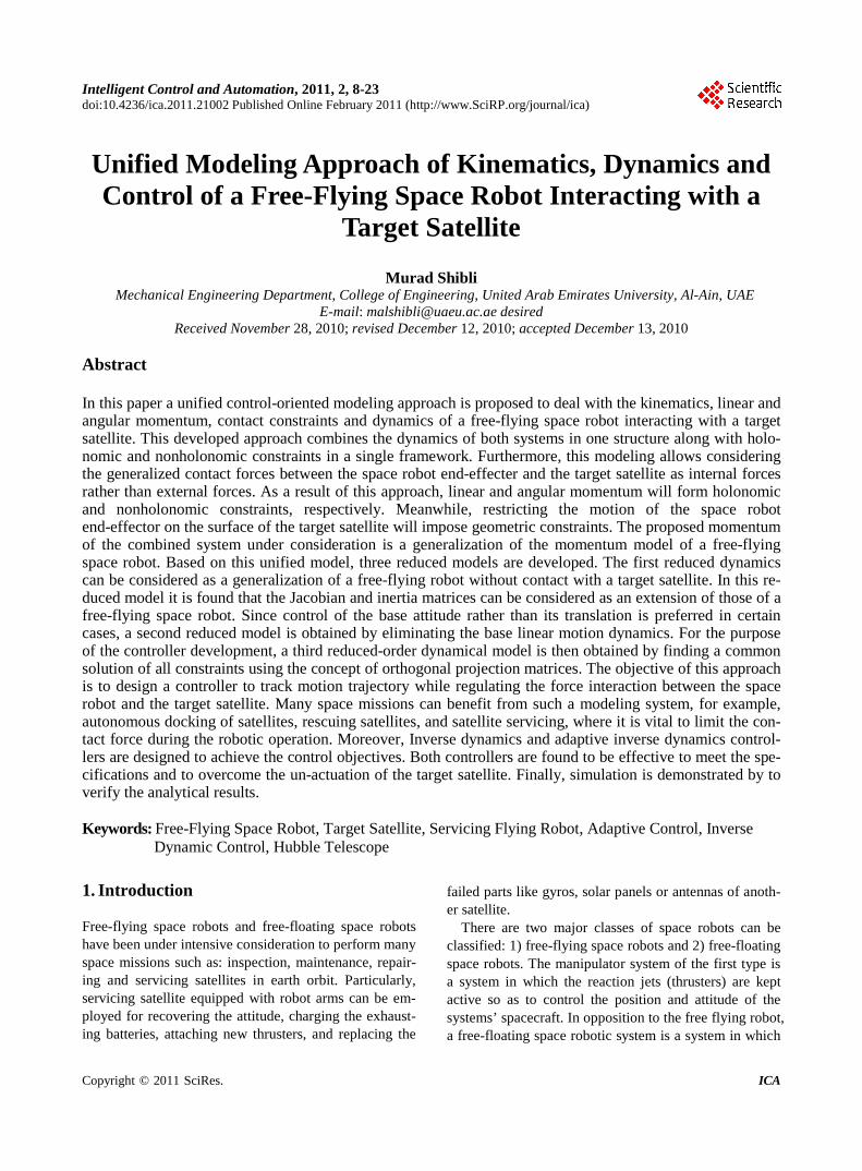
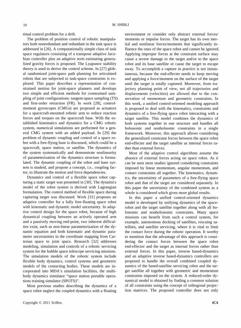
Our combined system can be modeled as a multi-body chain system composed of n + 2 rigid bodies. While the manipulator links are numbered from 1 to n, the base satellite (body 0) is denoted by b, in particular, and the ( )1n th+ body (the target satellite) by T. Moreover, This multi-body system is connected by n + 1 joints, which are given numbers from 1 to n + 1. Where the end-effecter is represented as the ( )1n th+ joint as shown in Figure 1.

We assume that all system bodies are rigid, the contact surfaces are frictionless and known. Also the effect of gravity gradient, solar radiation and aerodynamic forces are weak and neglected. It is assumed also that the base satellite is reaction-wheel actuated.

Referring to Figure 1, the position vector of the ith body centroid with respect to the inertial frame can be expressed as

i b i bR R R= + (1)

where the relative vector /biR is the position of the ith

body centroid with respect to the base frame [35,36]. Upon differentiating both sides of (1) with respect to

time, the relationship between the ith body velocity

i b b i b iV V R v= +Ω × + (2)

where iv is the linear velocities of the ith body in base coordinates. Now in the case of any ith body of the ma-nipulator, the velocity iv can be expressed in terms of the linear Jacobian matrix as

ii Lv J q= (3)

where

( ) ( ) ( )1 1 2 2, , , ,0, ,0iL i i i i iJ z R r z R r z R r = × − × − × −

(4)

Link i

Link n

Link 2

Link 1 O1

O2 q1

q2

q3 O3

Oi qi

i bR

Oi + 1

qi + 1

On qn

On + 1

qh

BΣ IΣ

CGΣ

TΣ

T EER

Figure 1. Free-floating space robot in contact with a target satellite.

M. SHIBLI

Copyright © 2011 SciRes. ICA

12

The end-effecter tip velocity is given by

EEEE b b EE b LV V R J q= +Ω × + (5)

Additionally, the velocity TV of the target satellite in the reference frame can be obtained by deriving Equation (1) as

TT b b T b L T T EE TV V R J q R vω= +Ω × + + × + (6)

Since the target satellite is not stationary, (6) shows the relative linear and angular velocities Tv , Tω be-tween the end effecter and the target satellite and meas-ured in the base frame.

Another relationship is needed between the ith body angular velocity iΩ and joint angular velocity

i b iωΩ = Ω + (7)

where iω is the angular velocities of the ith body in base coordinates and iω in case of the manipulator is given by

ii AJ qω = (8)

where the angular Jacobian

[ ]1 2, , , ,0, ,0iA iJ z z z= (9)

While in the case of the target satellite, the absolute angular velocity of can be expressed as

TT b A TJ q ωΩ = Ω + + (10)

Former analysis will be used in the next analysis to derive the momentum of s free-flying space robot. 2.3. Linear and Angular Momentum The linear and angular momentum of a multi-body sys-tem is a key part in understanding the motion of the sys-tem when it is not subjected to external forces. They may impose kinematic-like constraints when the system is free of any external force.

The linear momentum P and angular momentum L of the whole system is given by

1

0

n

i ii

P mV+

=

≡ ∑ (11)

( )1

0

nB

i i i i ii

L I m R V+

=

≡ Ω + ×∑ (12)

By means of (2-10), linear and angular momentum in (11-12) can then be represented in a compact form as

b b b b

V b bb b

b T b T

b T b T

V V V qbT

b q

V V v T

Tv

M M MVPq

M ML M

M M

vM Mω

ω

ω

Ω

Ω

Ω Ω

Ω Ω

= + Ω

+

(13)

where each block of the matrix is defined as follows 1

3 33

0b

n

V ii

M U m R+

×

=

≡ ∈∑ (14)

/

13 3

0,b b i b

n

V ii i b

M m R R+

×Ω

= ≠

≡ − × ∈ ∑ (15)

13

0,b Li

nn

V q ii i b

M m J R+

×

= ≠

≡ ∈∑ (16)

/

13 3

0,( )

b i b

n

i i bi i b

M I m D R I R+

×Ω

= ≠

≡ + + ∈∑ (17)

/

13

0,b A b Li i

nB n

q i i ii i b

M I J m R J R+

×Ω

= ≠

≡ + × ∈ ∑ (18)

1 /

3 3b T n EEV TM m R Rω +

× ≡ − × ∈ (19)

/

3 31( )

b T T EE

bi nM m D R I Rω

×Ω +≡ + ∈ (20)

3 33 1b TV v nM U m R ×

+≡ ∈ (21)

[ ]1

3 31b T nv nM m R R

+

×Ω +≡ − × ∈ (22)

Note that the matrix function [ ]R× for a vector , ,

Tx y zR R R R = is defined as

[ ] 3 3

00

0

z y

z x

y x

R RR R R R

R R

×

− × ≡ − ∈ −

(23)

and

[ ] [ ]2 2

2 2 3 3

2 2

( )

T

y z x y x z

x y x z y z

x z y z x y

D R R R

R R R R R RR R R R R R RR R R R R R

×

≡ × ×

+ − −

= − + − ∈ − − +

(24)

and the sub-matrices of the Jacobian of the ith body representing the linear and angular parts are defined be-fore.

Note that as in (13) the system is subjected to a non-holonomic (non-integrable) constraint because of con-servation of angular momentum in the absence of exter-nal forces. Note that the momentum constraints are not purely kinematical because of the inertial characteristics it carries in. Thus, this constraint is called kinematics- like. The physical meaning behind these constraints is that they restrict the kinematically possible displace-ments (possible velocities) of the individual parts of the system. On the contrast, the linear momentum results in a holonomic (integrable) constraint.

Now assuming zero initial conditions then linear and angular momentum is give by

M. SHIBLI

Copyright © 2011 SciRes. ICA

13

00

b b b b

V b bb b

b T b T

b T b T

V V V qbT

b q

V V v T

Tv

M M MVq

M M M

M M

vM Mω

ω

ω

Ω

Ω

Ω Ω

Ω Ω

= + Ω

+

(25)

Then it is possible that the relative linear and angular velocities of the target satellite can calculated as

1

1

b b bb T b T

V bb T b T b b

b T b T b

b T b T b

V VV V v bTT

bT v

V V v V q

v q

M MM M VM Mv M M

M M Mq

M M M

ω

ω

ω

ω

ω

Ω

−Ω

ΩΩ Ω

−

Ω Ω Ω

= − Ω

−

(26)

Equations (26) enables us to calculate the target veloc-ities [ ] T Tvω without measurements. 2.4. Contact Constraints We assume that the end-effecter moves on a sub-surface of the target satellite S and the profile of this surface is known so that it can be defined as

( ): , , , , , .S F x y z c constα β γ = = (27)

Let χ be the vector of generalized coordinates of the robot end-effecter in the target frame. The end-effecter, as a result of the contact with the target, is subjected to holonomic kinematic constraints defined in the constraint frame as

( ) 0χΦ = (28)

where ( ) : n mR RΦ ⋅ → is twice differentiable. The robot joint and target coordinates are related through the for-ward kienmatic function

( )f qχ = (29)

Now differentiating (28) with respect to time gives

( )0

χχ

χ∂Φ

=∂

(30)

Also differentiating (29) with respect to time

( )f qq

qχ

∂=

∂ (31)

Substituting (31) into (30) (chain rule) yields to

( ) ( )0

f qq

qχχ

∂Φ ∂=

∂ ∂ (32)

where the matrix ( ) ( )f q

Jqθ

χχ

∂Φ ∂=

∂ ∂ is the Jacobian

matrix

2.5. Common Solution of the Constraints In this section we study the constraints on a space robot in contact with a target satellite in one form. This entire system is subjected to holonomic and nonholonomic constraints at the same time. These Holonomic constraint are usually given in algebraic form relating the genera-lized variables (28). Now differentiating the holonomic constraint at the velocity level as in (30-32) leads to

( ) 0Jθ θ θ = (33)

where ( )Jθ θ is the Jacobian of the holonomic con-straint as defined in (32).

On the other hand, the conservation of momentum holds two types of constraints: linear momentum which is holnomic; and nonholnomic constraints come into play as a result of the conservation of the angular momentum. These momentum constraints are not given in algebraic form, but there are given in kinematical-like form as in (13) and can be rewritten in a compact form as

( ) 0B cθ θ = (34)

where 0c represents the vector of the initial conditions of the momentum. Equation (34) has k momentum con-straint equations with k N≤ , where N is number of generalized coordinates. The purpose of representing holonomic constraints in the form (33) is to treat both holonomic and nonholonmic constraints at the same dif-ferential level. But a difference exists in the matter of initial conditions. Holonomic constraints are restricted to position initial conditions, but nonholonomic are only restricted to their momentum conditions.

Now, all holonomic and nonholonomic constraints can be combined together as

( )( ) 0

0JcB

θ θθ

θ

=

(35)

where the new combined matrix ( ) ( )TT TJ Bθ θ θ

is of dimension ( ) ( )1k m n+ × + . This implies a set of ( )k m+ linear equations with θ as vector of the gene-ralized variables. Since matrices ( )Jθ θ and ( )B θ have the same number of columns, we now seek for their common solutions, if exist, expressing them in terms of the solutions of (33) and (34). The common solutions of (33) and (34) are the solutions of the combined con-straints (35). From the theory of linear algebra, the solu-tions of Equations (33) and (34) constitute the intersec-tion manifold

( ) ( ) N J B c N Bθ+ + (36)

where ( )N Jθ and ( )N B are the null space of Jθ and B, respectively. And the upper right script +

M. SHIBLI

Copyright © 2011 SciRes. ICA

14

represents the Pseudoinverse. Equation (36) is the set of solutions of (33) and (34) is consistent if (36) is non-empty. Then the common solution [36] is the manifolds

(a) ( ) ( ) ( )( ) ( ) ( )0N BN J N JP P P B c N J N Bθ θ θ

+++ + + (37)

(b) ( ) ( )( )

( ) ( )0 ( ) 0

N B N BN JB c P P P B c

N J N Bθ

θ

++ += − +

+ + (38)

(c) ( ) ( ) ( )0J J B B B c N J N Bθ θ θ

++ + += + + (39)

where ( )NP ⋅ is the projection matrix on the null space of a given matrix ( )⋅ .

Since each of the manifolds given in (37)-(39) give a solution of the combined system (35), these expressions can also be used to get the generalized (pseudo-inverse) of the combined matrices. Each of the following expres- sions is a 1,2,4 − inverse of the combined matrix

( ) ( )TT TJ Bθ θ θ

:

(d) ( ) ( ) ( )( )0 N BN J N JX J P P P J Bθ θθ θ

++ + + = + + −

(40)

(e) ( ) ( ) ( )( )0 N B N BN JY B P P P J Bθ θ

++ + + = − + −

(41)

( f) ( )Z J J B B J Bθ θ θ

++ + + + = + (42)

Moreover, if

( ) ( ) 0R J R Bθ∗ ∗ = (43)

then each expressions of (40-42) is the Moore-Penrose

inverse of ( ) ( ) TT TJ Bθ θ θ

.

3. Generalized Dynamics Modeling To drive the dynamic equation of a space robot interact-ing with a target, the total system kinetic energy as the total summation of the transitional and rotational energy of each body in the system can be expressed as

( )1

0

12 i

nT T b

i i i i ii

T mV V I+

=

≡ +Ω Ω∑ (44)

where iV and iΩ is the transitional and rotational velocities of i-th body , respectively, or it can be rear-ranged

[ ]1 2 b b T TT V q vω= Ω

b b b b b T b T

V b b b T b Tb b

V q q T Tb b

V q T T Tb T b T T

V v v qv v Tb T b T T T T

V V V q V V vbT

q vb

T Tq q qv

T T TTv

T T T T Tv

M M M M MV

M M M M M

M M M M M qM M M M M

vM M M M Mω ω ω

ω

ω

ω

ω

ω ω ω

Ω

Ω

Ω

Ω

Ω

Ω Ω Ω Ω

Ω ×

(45) where the block matrix in (45) is the inertia matrix and the sub-matrices are defined previously in (14-22) and also

( ) ( )1

1 1

0,i i

nn nT B T

q i Li L i Ai Ai i b

M m J J I J J R+

+ × +

= ≠

≡ ⋅ + ∈∑

(46)

( )/

3 31 1T T EEn nM I m D R Rω

×+ +≡ + ∈ (47)

( )3 11 1T T EE

nT T Tq n AT n LTM I J m J R Rω

× ++ +

≡ + × ∈

(48) ( )3 1

1T

nTqv n LTM m J U R × +

+≡ ∈ (49)

3 31T Tv n T EEM m R Rω

×+ ≡ − × ∈ (50)

3 33 1Tv nM U m R ×

+≡ ∈ (51)

Note that the inertia matrix M defined in (45) is sym-metric positive definite. Now define

T T

T T T T Tb bV q vθ ω = Ω (52)

Then the total kinetic energy can be expresses in a compact from

( )12

TT Mθ θ θ= (53)

From the kinetic energy formulation, the dynamics equations can be derived by using the Lagrangian ap-proach. Since there is no potential energy accounted in our system, the Lagrange function L is equal to the ki-netic energy T then becomes

Td T T Jdt

τ λθθ

∂ ∂− = +∂∂

(54)

where λ is the vector of unknown Lagrangian multip-liers.

The holonomic constraints are behind the generalized constraint forces as a result of the contact between the manipulator end-effecter and the surface of the target satellite. The combined system dynamics model can be represented as (assuming the target satellite is unac-tauted)

M. SHIBLI

Copyright © 2011 SciRes. ICA

15

0b b b b b T b T

V b b b T b Tb b b

V q q T Tb b

TV q T T Tb T b T T

TV v v qv v Tb T b T T T T

V V V q V V v VbT

q vb

T Tq q qv q

T T TwTv

T T T T T vv

M M M M M CVM M M M M CM M M M M Cq

CM M M M Mv CM M M M M

ω ω ω

ω

ω

ω

ω

ω ω ω

Ω

Ω

Ω

Ω

Ω

Ω Ω Ω Ω Ω

Ω +

00

T

T

TbLbLTbAbAT

TTwTTv

JFJFJ

J

J

θ λτ

= +

(55) The dynamic developed in (55) along with the com-

bined constraints in (35) completes the overall modeling of a space robot interacting with a target satellite. 4. Inverse Dynamics Control The basic idea of inverse dynamics control is to seek a nonlinear dynamics control law that cancels exactly all nonlinear terms in the system dynamics (55) so that the closed loop dynamics is linear and decoupled [6].

Now assuming zero initial conditions in (13) and (35), the overall dynamics subjected to the constraints can be expressed in a compact form as

cM C Fθ θ τ+ = + (56)

where the inertia matrix M is defined in (55), the nonli-near vector ( ),C θ θ is the centrifugal/Coriolos forces the generalized constraint forces are T

cF J λ= , mRλ ∈ is the vector of unknown Lagrangian multipliers, TJ and τ are defined, respectively, as

t

t

TbLTbATTq

TTwTTv

JJJJJ

J

=

,

00

L

A

b

b

F

Fτ τ

=

as in (55), and finally the

constraint matrix ( ) ( )( )

JA

Bθ θ

θθ

=

as given in (35).

In the constraint Equation (35) there are ( )k m+ li-near equations and N of the generalized velocities θ . It clear that there are fewer equations than unknowns, this implies the existence of infinite solutions. From the theory of linear algebra, the solution of (35) can be given by

( )Sθ θ ν= (57)

where ( ) ( ) ( )N N k mS Rθ × − −∈ is an orthogonal projector of

full rank and belong to the null space of ( )A q and the vector ( )N k mRν − −∈ can be chosen arbitrary. It implies that 0TS A = . [37]

Now differentiating (57) at the acceleration level with respect to time yields

S Sθ ν ν= +

(58) Upon substituting the velocities (57) and the accelera-

tion (58) into the dynamics (55) we obtain

( ) cMS MS CS Fν ν τ+ + = +

(59)

Let us define the controller as τ

( ) ( ) Td D P cHS CS HS K e K e Jτ ν ν λ= + + + + −

(60)

where the position tracking error is defined as p de ν ν= − and cλ is defined as

c d F F I FK e K e dtλ λ= − − ∫ (61)

where F de λ λ= − and the gain matrices PK , DK , FK and IK are chosen as diagonal with positive ele-

ments. Note that the input to the proposed controller (60) are

the joint angles and velocities, angular velocity of the base, relative velocities of both satellites, contact forces and the output of the controller is the joint torques. Note also that T N k ms Rτ − −∈ has the advantage of overcom-ing the underactuation of the system as a result of target satellite jet shutdown or failure, and the inputs provided by the robot and the base is enough to control the whole system. This is because the number of constraints k m+ ≥ the number of passive inputs of the target satel-lite.

Now let us substitute the control law (60) into the dy-namics (59), then, the closed loop dynamics is given by

( )( )

0

Tp D p P p

T TF F I F

S MS e K e K e

S J K e K e dt

+ +

= − +

=∫

(62)

Since J belongs to the null space of S, that is, 0T TS J = and since by the virtue of (57), the projection

matrix ( )S q and its transpose are of full rank, and the inertia matrix is symmetric positive definite, then

TS MS is also a positive definite. Now we need to verify the terms inside the brackets in (60) are zero. This condi-tion can be guaranteed by choosing the proper positive gains DK and PK such that dν ν→ as t →∞ . If the gain matrices DK and PK are chosen as diagonal with positive diagonal elements, then the resulted closed loop dynamics is linear, decoupled and exponentially stable. Global stability can then be guaranteed. The closed loop dynamics natural frequency and damping ration can be chosen to meet specific requirements. Also

M. SHIBLI

Copyright © 2011 SciRes. ICA

16

by inspecting the right hand side we can see that the

F F I FK e K e dt+ ∫ can be guaranteed to be zero by choosing the suitable gain matrices FK and IK .

Now we can readily summarize the hybrid inverse- dynamics controller in the following theorem:

Theorem 1: For the dynamic system given in (59) and subjected to constraints (35), the inverse dynamics con-trol law defined by (60)-(61) is globally stable and guar-antees zero steady state and force tracking errors.

To further improve the dynamic response in case of system parameters uncertainty, an adaptive controller would serve that objective as in the nest section. 5. Adaptive Inverse Dynamics Control Similar to the analysis followed in the previous section and recalling (60)

( ) THS HS CS Jν ν τ λ+ + = +

(63)

Now we assume that there are some uncertainties in the system parameters such as masses and inertias and for this reason an adaptive control approach will be investigated. The dynamics (63) can be represented by benefiting from the property of linearity in parameters as [38,39]

1 1H Cν ν α+ = Υ (64)

where 1H HS= , ( )1C HS CS= + , Y is an ( )N N m× − matrix of known functions and known is the regressor, and α is an ( )N m− -dimensional vector of the sys-tem parameters. After examining the structure of dy-namics (55), three properties are obtained:

Property 1: The modified inertia matrix ( ) ( ) ( )2

TH S H Sθ θ θ= is symmetric positive definite.

Property 2: If Property 1 is verified, then ( )2 22H C− is skew-symmetric matrix where 2 1

TC S C= . Property 3: The dynamics (64) is linear in its parame-

ters. The nonlinear control law is proposed to have the form

( )1 1ˆˆ T

d D P cH K e K e C Jτ ν ν λ= + + + − (65)

where c d F FK eλ λ= − and FK is a positive definite diagonal matrix for the force control feedback gain and

F de λ λ= − , and where 1H and 1C are the estimates of 1H and 1C , respectively. Note that the geometric of the Jacobian in (56) is assumed to be determined.

Then the dynamics (55) can be modified to

1 1ˆˆ ˆH Cν ν α+ = Υ (66)

where α is the estimated vector of parametersα . Upon substituting (65) into (63), and by adding and

subtracting at the same time the term 1M v on the left hand side of (65) we get

( ) ( )1 1 1 1

1 1

ˆˆ

ˆˆ T Td D P c

H H H C

H K e K e C S J

ν ν ν ν

ν ν λ λ

− + +

= + + + − −

(67)

Rearranging (58) and canceling out the similar terms, yields

( )1 1 1 1

1 1

ˆˆ

ˆˆd D P P P

H H C C

H K e K e HY

ν ν ν ν

ν ν ν

α

− + −

= − + + −

=

(68)

or,

( )1 1 1ˆ

P D P P PH C H e K e K e Yν ν α+ = + + =

(69)

where P de ν ν= − , and ( ) ( ) ( )ˆ⋅ = ⋅ − ⋅

. The closed loop dynamics error can be written as

( ) 1P D P P Pe K e K e Yα+ + = (70)

where 11 1H Y Y− = .

It is possible now to express the error dynamics (70) in a state space form as

x Ax Bα= + (71) where

1

, , p

p P D

e O I Ox A B

e K K Y

= = = − − (72)

where A is a Hurwitz matrix, that is, the real parts of its eigenvalues are negative, which guarantees globally ex-ponentially stability. Based on the state space formula-tion and Lyapunov techniques an adaptive control law can be chosen as

11T TY B Pxα −= −Γ

(73)

where 0Γ > and symmetric , and P is a unique positive definite solution to the Lyapunov equation TA P PA+ =

Q− where Q is a positive definite symmetric. Proof: Let the Lyaponuv candidate function chosen as

T TV x Px α α= + Γ (74) Now if take the time derivative of V along the trajec-

tories of (71) and by using the adaptation law (65), one gets

( ) ( )

( )

( )

1 1

1 11 1

1 1

11 1

1

1 1 1

T T T T

T T

TT T T T T

T T T T T T T

T T T T T T

T T T T T

T T T T T

V x Px x Px

Ax BY Px x P Ax BY

Y B Px Y B Px

x A Px Y B Px x PAx x PBY

x P BY Y B Px

x A P PA x Y B Px

x P BY x P BY Y

α α α α

α α

α α

α α

α α

α

α α α

− −

− −

= + + Γ + Γ

= + + +

− Γ Γ − Γ Γ

= + + +

− Γ Γ − Γ Γ

= + +

+ − −

T TB Px

(75)

M. SHIBLI

Copyright © 2011 SciRes. ICA

17

By canceling out equivalent terms, this reduces to

0TV x Qx= − ≤ (76)

Since V is negative semidefinite with regard to x and the parameter error, and V is lower bounded by zero, V remains bounded in the time interval [ )0,∞ . This fact can be stated as

0Vdt

∞− < ∞∫ (77)

Now if we assume that x is bounded then from (74) V is bonded. If V is bounded then V is uniformly continuous. If V is uniformly continuous and has a fi-nite integral as given in (76) then by Barbalat’s lemma

0V → as t →∞ which implies 0x → as t →∞ . Substituting the control law (65) and (73) into the dy-

namics (55) yields

( )TcJ Yλ λ α σ− = − = (78)

where σ is a bounded function. Thus

( ) 1TF FJ e K I σ−= + (79)

and the force tracking error ( )dF F− is bounded and can be adjusted by changing the feedback gain FK . Thus, the previous adaptive algorithm can be concluded in the following theorem:

Theorem 2: For the dynamic system given in (63) and subjected to constraints (35), the adaptive control law defined by (69) and (73) is globally stable and guarantees zero steady state and force tracking errors. 6. Simulation Results This section will demonstrate the kinematics, dynamics and controller presented in this paper as follows.

Part A (PD controller): A 6-DOF space robot arm mounted on a base satellite is used to demonstrate the analytical results. We assume that the end-effecter estab-lished a contact with a target satellite. This target satellite is assumed to be totally floating and unactuated due to the thrusters’ failure. The mass of the base servicing sa-tellite is chosen as 300 kg, the masses of the 6-robot arm as [20 20 15 10 10 10] kg, and 1000 kg for the target satellite. The initial linear velocities of both the base and the target are assumed to be 10 m/sec to keep a constant linear relative velocity while conducting the task and to avoid any damage. Two different PD controllers are used, to control the base satellite reaction wheels and robot

arm as: ( ),rw P b b des D bk A A kτ = − + Ω , ( )1 2arm desk q q k qτ = − − ,

respectively, where [ ]10 10 10 TPk = , [ ]10 10 10 T

Dk = , 1 10k = , 2 10k = . The simulation results are shown in

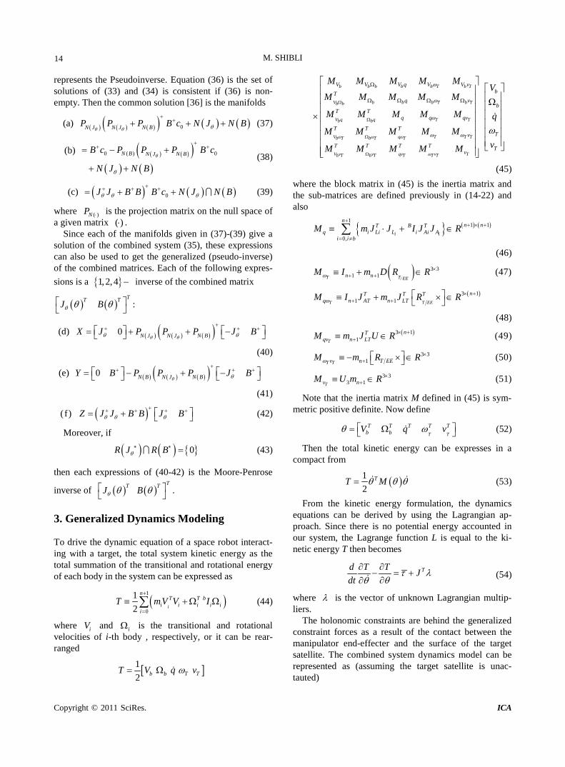
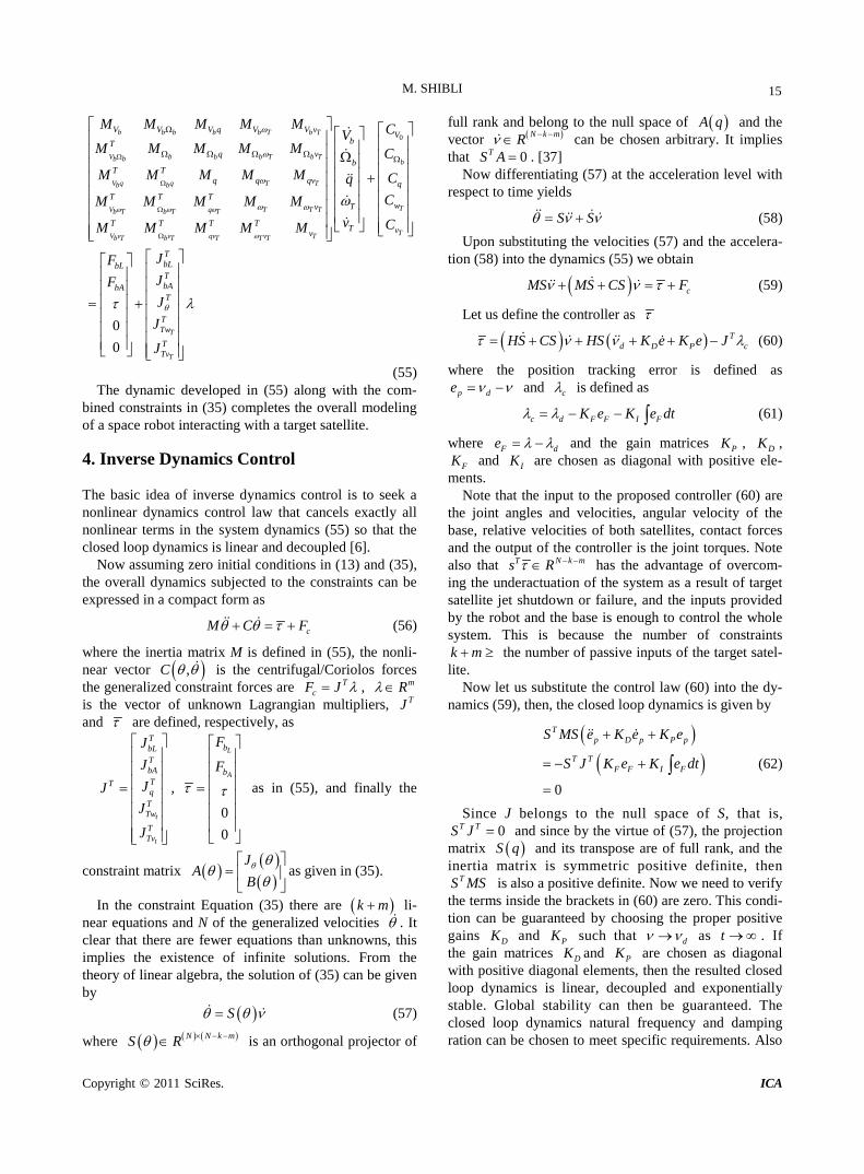
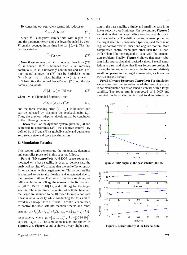
Figures 2-6. Figures 2 and 3 shows a very slight varia-

tion in the base satellite attitude and small increase in its linear velocity over 3 minutes. On the contrast, Figures 5 and 6 show that the target drifts away, but a slight rise in its linear velocity. The drift is due to the assumption that the target satellite is unactuated (passive) and there is no regular control over its linear and angular motion. More complicated control techniques other than the PD con-troller should be investigated to cope with the unactua-tion problem. Finally, Figure 4 shows that most robot arm links approaches their desired values. Several simu-lations are run and show that linear forces are preferable on angular forces, and as long as the forces are relatively small comparing to the target mass/inertia, its linear ve-locities slightly change.

Part B (Inverse Dynamics Controller): For simulation we assume that the end-effecter of the servicing space robot manipulator has established a contact with a target satellite. The robot arm is composed of 6-DOF and mounted on base satellite is used to demonstrate the

time, sec

w0,

rad/

sec

× 10-3 0.5

0

–0.5

–1

–1.5

–2

–2.5

–3 0 20 40 60 80 100 120

Figure 2. YRP-angles of the base satellite (10e-3).

time, sec

v 0z,

m/s

ec

10.05

0 20 40 60 80 100 120

time, sec 0 20 40 60 80 100 120

time, sec 0 20 40 60 80 100 120

10

9.95

0.01

0

–0.01

0.02

0.01

0

v 0y,

m/s

ec

v 0x,

m/s

ec

Figure 3. Linear velocity of the base satellite.

M. SHIBLI

Copyright © 2011 SciRes. ICA

18

time, sec

q(t)

1.2

–0.2 0 20 40 60 80 100 120

1

0.8

0.6

0.4

0.2

0

Figure 4. Robot arm angles.

time, sec

w1,

rad/

sec

0.45

–0.05 0 20 40 60 80 100 120

0.05

0

0.1

0.15

0.2

0.25

0.3

0.35

0.4

Figure 5. YRP-angles of the target satellite.

v tz',

m/se

c

10.05

time, sec 0 20 40 60 80 100 120 10

0.04

v ty', m

/sec

v t

x', m

/sec

time, sec 0 20 40 60 80 100 120

time, sec 0 20 40 60 80 100 120

0.02

0

0.04

0.02

0

10.1

Figure 6. Linear velocity of the target satellite.

analytical results. This target satellite is assumed to be totally floating and unactuated due to the thrusters’ fail-ure. The mass of the base servicing satellite is chosen as

300 kg, the masses of the 6-robot arm as [10 10 10 10 10 10] kg, and 1500 kg for the target satellite. The initial linear velocities of both the base and the target are as-sumed to be 20 m/sec to keep a constant linear relative velocity while conducting the task and to avoid any damage. All other initial conditions are assumed to be zero.

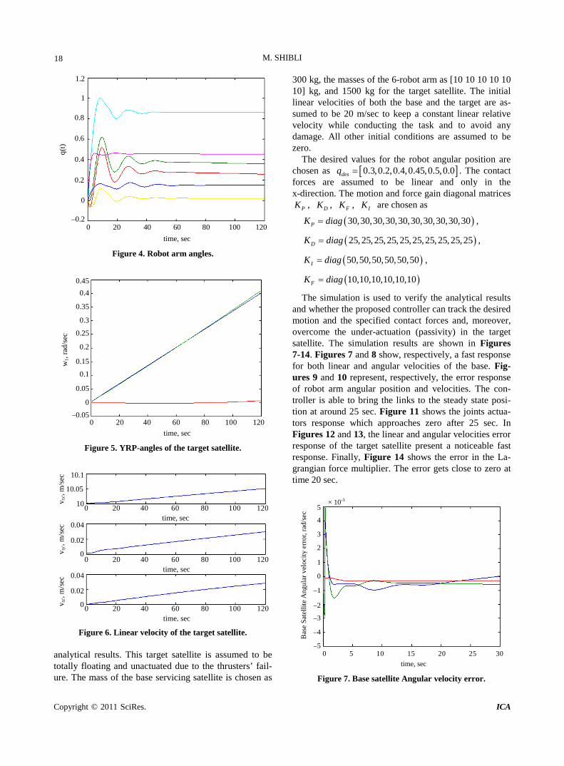
The desired values for the robot angular position are chosen as [ ]0.3,0.2,0.4,0.45,0.5,0.0desq = . The contact forces are assumed to be linear and only in the x-direction. The motion and force gain diagonal matrices

PK , DK , FK , IK are chosen as

( )30,30,30,30,30,30,30,30,30,30PK diag= ,

( )25,25,25,25,25,25,25,25,25,25DK diag= ,

( )50,50,50,50,50,50IK diag= ,

( )10,10,10,10,10,10FK diag=

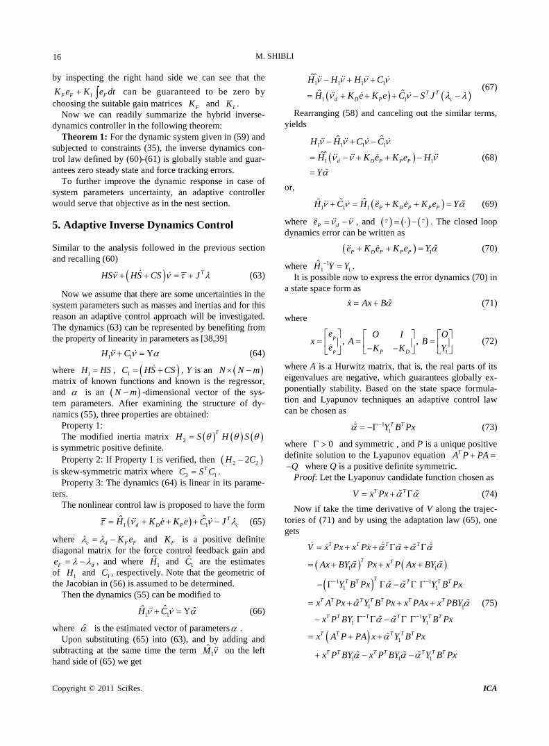
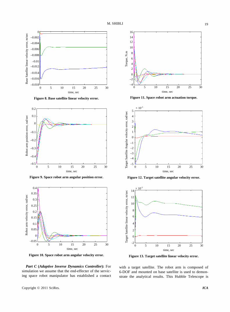
The simulation is used to verify the analytical results and whether the proposed controller can track the desired motion and the specified contact forces and, moreover, overcome the under-actuation (passivity) in the target satellite. The simulation results are shown in Figures 7-14. Figures 7 and 8 show, respectively, a fast response for both linear and angular velocities of the base. Fig-ures 9 and 10 represent, respectively, the error response of robot arm angular position and velocities. The con-troller is able to bring the links to the steady state posi-tion at around 25 sec. Figure 11 shows the joints actua-tors response which approaches zero after 25 sec. In Figures 12 and 13, the linear and angular velocities error response of the target satellite present a noticeable fast response. Finally, Figure 14 shows the error in the La-grangian force multiplier. The error gets close to zero at time 20 sec.

time, sec

Bas

e Sa

telli

te A

ngul

ar v

eloc

ity e

rror,

rad/

sec

× 10-3 5

–5 0 5 10 15 20 25 30

4

3

2

1

0

–4

–3

–2

–1

Figure 7. Base satellite Angular velocity error.

M. SHIBLI

Copyright © 2011 SciRes. ICA

19

time, sec

Bas

e Sa

telli

te li

near

vel

ocity

erro

r, m

/sec

0

–0.002

0 5 10 15 20 25 30

–0.004

–0.006

–0.008

–0.01 –0.012

–0.014

–0.016

–0.018

Figure 8. Base satellite linear velocity error.

time, sec

Rob

ot a

rm p

ositi

on e

rror,

rad/

sec

0.2

0 5 10 15 20 25 30 –0.5

0.1

0

–0.4

–0.3

–0.2

–0.1

Figure 9. Space robot arm angular position error.

time, sec

Rob

ot a

rm v

eloc

ity e

rror,

rad/

sec

0.4

0 5 10 15 20 25 30 –0.05

0.35

0.3

0.25

0.2

0.15

0.1

0.05

0

Figure 10. Space robot arm angular velocity error.

Part C (Adaptive Inverse Dynamics Controller): For

simulation we assume that the end-effecter of the servic-ing space robot manipulator has established a contact

time, sec

Torq

ue, N

.m

16

0 5 10 15 20 25 30

–2

14 12

10

8

6

4 2

0

–4

Figure 11. Space robot arm actuation torque.

time, sec

Targ

et S

atel

lite A

ngul

ar v

eloc

ity e

rror,

rad/

sec 5

0 5 10 15 20 25 30

–1

× 10-3

4

3

2

1

0

–2

–3 –4

–5

Figure 12. Target satellite angular velocity error.

time, sec

Targ

et S

atel

lite

linea

r vel

ocity

erro

r, m

/sec

14

0 5 10 15 20 25 30

× 10-3

12

10

8

6

4

2

0

-2

Figure 13. Target satellite linear velocity error.

with a target satellite. The robot arm is composed of 6-DOF and mounted on base satellite is used to demon-strate the analytical results. This Hubble Telescope is

M. SHIBLI

Copyright © 2011 SciRes. ICA

20

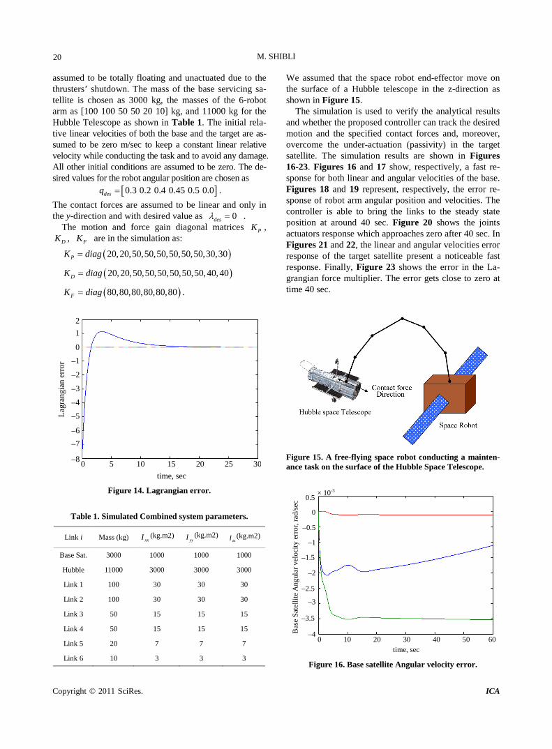
assumed to be totally floating and unactuated due to the thrusters’ shutdown. The mass of the base servicing sa-tellite is chosen as 3000 kg, the masses of the 6-robot arm as [100 100 50 50 20 10] kg, and 11000 kg for the Hubble Telescope as shown in Table 1. The initial rela-tive linear velocities of both the base and the target are as-sumed to be zero m/sec to keep a constant linear relative velocity while conducting the task and to avoid any damage. All other initial conditions are assumed to be zero. The de-sired values for the robot angular position are chosen as

[ ]0.3 0.2 0.4 0.45 0.5 0.0desq = . The contact forces are assumed to be linear and only in the y-direction and with desired value as 0desλ = .

The motion and force gain diagonal matrices PK , DK , FK are in the simulation as:

( )20,20,50,50,50,50,50,50,30,30PK diag=

( )20,20,50,50,50,50,50,50,40,40DK diag=

( )80,80,80,80,80,80FK diag= .

time, sec

Lagr

angi

an e

rror

2

0 5 10 15 20 25 30

1

0 –1

–2

–3

–4

–5

–6 –7

–8

Figure 14. Lagrangian error.

Table 1. Simulated Combined system parameters.

Link i Mass (kg) xxI (kg.m2) yyI (kg.m2)

zzI (kg.m2)

Base Sat. 3000 1000 1000 1000

Hubble 11000 3000 3000 3000

Link 1 100 30 30 30

Link 2 100 30 30 30

Link 3 50 15 15 15

Link 4 50 15 15 15

Link 5 20 7 7 7

Link 6 10 3 3 3

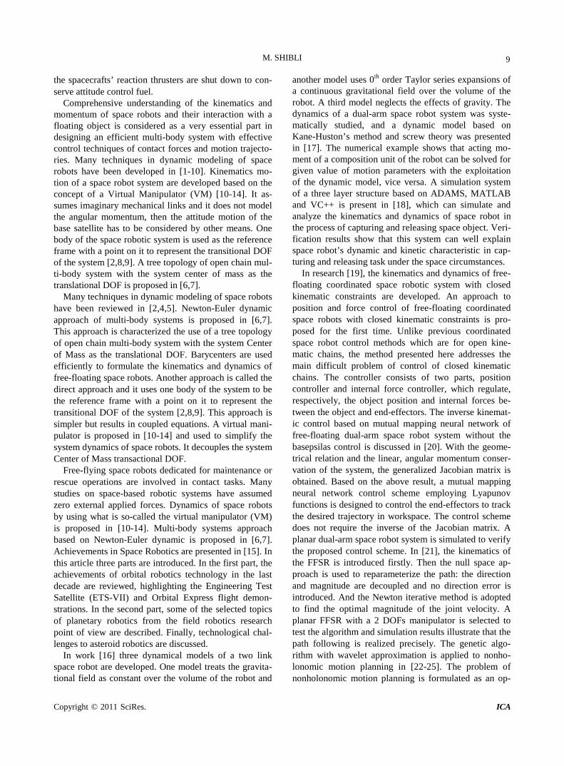
We assumed that the space robot end-effector move on the surface of a Hubble telescope in the z-direction as shown in Figure 15.

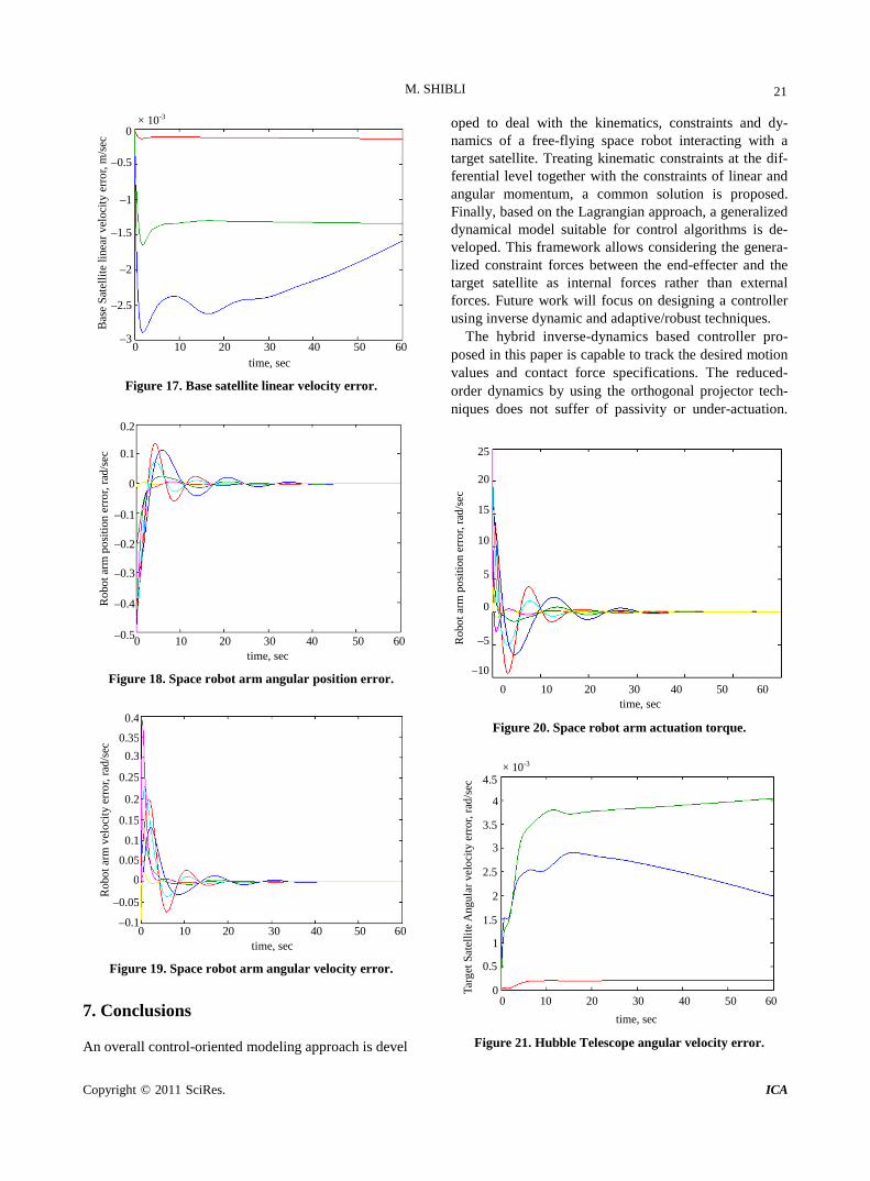
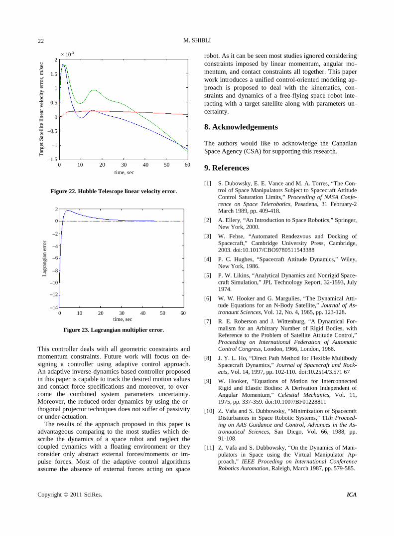
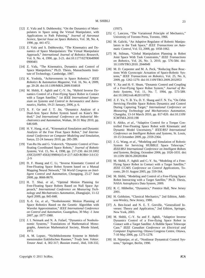
The simulation is used to verify the analytical results and whether the proposed controller can track the desired motion and the specified contact forces and, moreover, overcome the under-actuation (passivity) in the target satellite. The simulation results are shown in Figures 16-23. Figures 16 and 17 show, respectively, a fast re-sponse for both linear and angular velocities of the base. Figures 18 and 19 represent, respectively, the error re-sponse of robot arm angular position and velocities. The controller is able to bring the links to the steady state position at around 40 sec. Figure 20 shows the joints actuators response which approaches zero after 40 sec. In Figures 21 and 22, the linear and angular velocities error response of the target satellite present a noticeable fast response. Finally, Figure 23 shows the error in the La-grangian force multiplier. The error gets close to zero at time 40 sec.

Figure 15. A free-flying space robot conducting a mainten-ance task on the surface of the Hubble Space Telescope.

time, sec

Bas

e Sa

telli

te A

ngul

ar v

eloc

ity e

rror,

rad/

sec

× 10-3 0.5

–0.5

0 10 20 30 40 50 60

0

–1

–1.5

–2

–2.5

–3

–3.5

–4

Figure 16. Base satellite Angular velocity error.

M. SHIBLI

Copyright © 2011 SciRes. ICA

21

time, sec

Bas

e Sa

telli

te li

near

vel

ocity

erro

r, m

/sec

× 10-3

–0.5

0 10 20 30 40 50 60

0

–1

–1.5

–2

–2.5

–3

Figure 17. Base satellite linear velocity error.

time, sec

Rob

ot a

rm p

ositi

on e

rror,

rad/

sec

–0.5 0 10 20 30 40 50 60

0.2

0.1

0

–0.1

–0.2

–0.3

–0.4

Figure 18. Space robot arm angular position error.

time, sec

Rob

ot a

rm v

eloc

ity e

rror

, rad

/sec

–0.1 0 10 20 30 40 50 60

0.4

0.35 0.3

0.25

0.2

0.15

0.1

0.05

0

–0.05

Figure 19. Space robot arm angular velocity error.

7. Conclusions An overall control-oriented modeling approach is devel

oped to deal with the kinematics, constraints and dy-namics of a free-flying space robot interacting with a target satellite. Treating kinematic constraints at the dif-ferential level together with the constraints of linear and angular momentum, a common solution is proposed. Finally, based on the Lagrangian approach, a generalized dynamical model suitable for control algorithms is de-veloped. This framework allows considering the genera-lized constraint forces between the end-effecter and the target satellite as internal forces rather than external forces. Future work will focus on designing a controller using inverse dynamic and adaptive/robust techniques.

The hybrid inverse-dynamics based controller pro-posed in this paper is capable to track the desired motion values and contact force specifications. The reduced- order dynamics by using the orthogonal projector tech-niques does not suffer of passivity or under-actuation.

time, sec

Rob

ot a

rm p

ositi

on e

rror,

rad/

sec

–5

0 10 20 30 40 50 60

25

20

15

10

5

0

–10

Figure 20. Space robot arm actuation torque.

time, sec

Targ

et S

atel

lite A

ngul

ar v

eloc

ity e

rror,

rad/

sec

× 10-3 4.5

0 10 20 30 40 50 60

4

3.5

3

2.5

2

1.5

1

0.5

0

Figure 21. Hubble Telescope angular velocity error.

M. SHIBLI

Copyright © 2011 SciRes. ICA

22

time, sec

Targ

et S

atel

lite

linea

r vel

ocity

erro

r, m

/sec

× 10-3 2

0 10 20 30 40 50 60

1.5

1

0.5

0

–0.5

–1

–1.5

Figure 22. Hubble Telescope linear velocity error.

time, sec

Lagr

angi

an e

rror

2

0 10 20 30 40 50 60

–12

0

–2

–4

–6

–8

–10

–14

Figure 23. Lagrangian multiplier error.

This controller deals with all geometric constraints and momentum constraints. Future work will focus on de-signing a controller using adaptive control approach. An adaptive inverse-dynamics based controller proposed in this paper is capable to track the desired motion values and contact force specifications and moreover, to over-come the combined system parameters uncertainty. Moreover, the reduced-order dynamics by using the or-thogonal projector techniques does not suffer of passivity or under-actuation.

The results of the approach proposed in this paper is advantageous comparing to the most studies which de-scribe the dynamics of a space robot and neglect the coupled dynamics with a floating environment or they consider only abstract external forces/moments or im-pulse forces. Most of the adaptive control algorithms assume the absence of external forces acting on space

robot. As it can be seen most studies ignored considering constraints imposed by linear momentum, angular mo-mentum, and contact constraints all together. This paper work introduces a unified control-oriented modeling ap-proach is proposed to deal with the kinematics, con-straints and dynamics of a free-flying space robot inte-racting with a target satellite along with parameters un-certainty. 8. Acknowledgements The authors would like to acknowledge the Canadian Space Agency (CSA) for supporting this research. 9. References [1] S. Dubowsky, E. E. Vance and M. A. Torres, “The Con-

trol of Space Manipulators Subject to Spacecraft Attitude Control Saturation Limits,” Proceeding of NASA Confe-rence on Space Telerobotics, Pasadena, 31 February-2 March 1989, pp. 409-418.

[2] A. Ellery, “An Introduction to Space Robotics,” Springer, New York, 2000.

[3] W. Fehse, “Automated Rendezvous and Docking of Spacecraft,” Cambridge University Press, Cambridge, 2003. doi:10.1017/CBO9780511543388

[4] P. C. Hughes, “Spacecraft Attitude Dynamics,” Wiley, New York, 1986.

[5] P. W. Likins, “Analytical Dynamics and Nonrigid Space-craft Simulation,” JPL Technology Report, 32-1593, July 1974.

[6] W. W. Hooker and G. Margulies, “The Dynamical Atti-tude Equations for an N-Body Satellite,” Journal of As-tronaunt Sciences, Vol. 12, No. 4, 1965, pp. 123-128.

[7] R. E. Roberson and J. Wittenburg, “A Dynamical For-malism for an Arbitrary Number of Rigid Bodies, with Reference to the Problem of Satellite Attitude Control,” Proceeding on International Federation of Automatic Control Congress, London, 1966, London, 1968.

[8] J. Y. L. Ho, “Direct Path Method for Flexible Multibody Spacecraft Dynamics,” Journal of Spacecraft and Rock-ects, Vol. 14, 1997, pp. 102-110. doi:10.2514/3.571 67

[9] W. Hooker, “Equations of Motion for Interconnected Rigid and Elastic Bodies: A Derivation Independent of Angular Momentum,” Celestial Mechanics, Vol. 11, 1975, pp. 337-359. doi:10.1007/BF01228811

[10] Z. Vafa and S. Dubbowsky, “Minimization of Spacecraft Disturbances in Space Robotic Systems,” 11th Proceed-ing on AAS Guidance and Control, Advances in the As-tronautical Sciences, San Diego, Vol. 66, 1988, pp. 91-108.

[11] Z. Vafa and S. Dubbowsky, “On the Dynamics of Mani-pulators in Space using the Virtual Manipulator Ap-proach,” IEEE Proceding on International Conference Robotics Automation, Raleigh, March 1987, pp. 579-585.

M. SHIBLI

Copyright © 2011 SciRes. ICA

23

[12] Z. Vafa and S. Dubbowsky, “On the Dynamics of Mani-pulators in Space using the Virtual Manipulator, with Applications to Path Palnning,” Journal of Astronaut Scence, Special Issue on Space Robotics, Vol. 38, No. 4, 1990, pp. 441-472.

[13] Z. Vafa and S. Dubbowsky, “The Kinematics and Dy-namics of Space Manipulators: The Virtual Manipulator Approach,” International Journal of Robotics Research, Vol. 9, No. 4, 1990, pp. 3-21. doi:10.1177/02783649900 0900401

[14] Z. Vafa, “The Kinematics, Dynamics and Control of Space Manipultors,” Ph.D. Thesis, Massachusetts Insti-tute of Technology, Cambridge, 1987.

[15] K. Yoshida, “Achievements in Space Robotics,” IEEE Robotics & Automation Magazine, Vol. 16, No. 4, 2009, pp. 20-28. doi:10.1109/MRA.2009.934818

[16] M. Shibli, F. Aghili and C.-Y. Su, “Hybrid Inverse Dy-namics Control of a Free-Flying Space Robot in Contact with a Target Satellite,” 1st IEEE International Sympo-sium on Systems and Control in Aeronautics and Astro-nautics, Harbin, 19-21 January, 2006, p. 6.

[17] X. F. Ge and J. T. Jin, “Dynamics Analyze of a Dual-Arm Space Robot System based on Kane's Me-thod,” 2nd International Conference on Industrial Me-chatronics and Automation, Wuhan, 30-31 May 2010, pp. 646-649.

[18] H. Y. Hang, et al., “Kinematical Simulation and Dynamic Analysis of the Free Float Space Robot,” 2nd Interna-tional Conference on Computer Modeling and Simulation, Sanya, 22-24 January 2010, pp. 285-289.

[19] Yan-Ru Hu and G. Vukovich, “Dynamic Control of Free- floating Coordinated Space Robots,” Journal of Robotic Systems, Vol. 15, No. 4, 1998, pp. 217-230. doi:10.1002 /(SICI)1097-4563(199804)15:4<217:AID-ROB4>3.0.CO;2-S

[20] D. F. Huang and C. Li, “Inverse Kinematic Control of Free-Floating Space Robot System based on a Mutual Mapping Neural Network,” 7th World Congress on Intel-ligent Control and Automation, Chongqing, 25-27 June 2008, pp. 8666-8670.

[21] H. T. Shui, et al., “Optimal Motion Planning for Free-Floating Space Robots Based on Null Space Ap-proach,” International Conference on Measuring Tech-nology and Mechatronics Automation, Zhangjiajie, 11-12 April 2009, pp. 845-848.

[22] X.-S. Ge, et al., “Nonholonomic Motion Planning of Space Robotics Based on the Genetic Algorithm with Wavelet Approximation,” IEEE International Conference on Control and Automation, Guangzhou, 30 May -1 June 2007, pp: 1977-1980.

[23] J. I. Neimark and N. A. Fufaef, “Dynamics of Nonholo-nomic Systems,” Translations of Mathematical Mono-graphs, American Mathematical Society, Rhode Island, 1972.

[24] A. M. Lopsec, “Nichthholomome Systeme in Mehrdi-mensionalen Euklidischen Raumen,” Trudy Sem. Vektor. Tenzor Anal. 4, 302-317; Russian transl., ibid, 318-332,

(1937). [25] C. Lanczos, “The Variational Principle of Mechanics,”

University of Toronto Press, Toronto, 1966. [26] M. Galicki, “An Adaptive Regulator of Robotic Manipu-

lators in the Task Space,” IEEE Transactions on Auto-matic Control, Vol. 53, 2008, pp. 1058-1062.

[27] M. Stilman, “Global Manipulation Planning in Robot Joint Space With Task Constraints,” IEEE Transactions on Robotics, Vol. 26, No. 3, 2010, pp. 576-584. doi: 10.1109/TRO.2010. 2044949

[28] M. D. Carpenter and M. A. Peck, “Reducing Base Reac-tions With Gyroscopic Actuation of Space-Robotic Sys-tems,” IEEE Transactions on Robotics, Vol. 25, No. 6, 2009, pp. 1262-1270. doi:10.1109/TRO.2009.2032953

[29] Y. Xu and H.-Y. Shum, “Dynamic Control and Coupling of a Free-Flying Space Robot System,” Journal of Ro-botic Systems, Vol. 11, No. 7, 1994, pp. 573-589. doi:10.1002/rob.4620110702

[30] Z. F. Yu, Y. B. Yu, D. Y. Shang and F. N. Yu, “On Orbit Servicing Flexible Space Robots Dynamics and Control During Capturing Target,” International Conference on Measuring Technology and Mechatronics Automation, Changsha, 13-14 March 2010, pp. 817-820. doi:10.1109/ ICMTMA.2010.198

[31] S. Abiko, et al., “Adaptive Control for a Torque Con-trolled Free-Floating Space Robot with Kinematic and Dynamic Model Uncertainty,” IEEE/RSJ International Conference on Intelligent Robots and Systems, St. Louis, 10-15 Octomber 2009, pp. 2359-2364.

[32] J. G. Wang, et al., “Modeling and Simulation of Robotic System for Servicing HUBBLE Space Telescope,” IEEE/RSJ International Conference on Intelligent Robots and Systems, Beijing, Octomber 2006, pp. 1026-1031. doi: 10.1109/ IROS.200281804

[33] M. Shibli, F. Aghili and C.-Y. Su, “Modeling of a Free- Flying Space Robot in Contact with a Target Satellite,” IEEE CCA05 Conference on Control Applications, To-ronto, 28-31 August 2005, pp. 559-564.

[34] M. Shibli, “Modeling and Control of a Free-Flying Space Robot Interacting with a Target Satellite,” Ph.D. Thesis, NASA Astrophysics Data System, 2009.

[35] R. C. Hibbeller, “Dynamics,” Prentice Hall, New Jersey 2001.

[36] H. Goldstien, “Classical Mechanics,” 2nd Edition, Addi-son-Wesley, New Jersey, 1980.

[37] A. Ben-Israel and N. E. T. Greville, “Generalized In-verses: Theory and Application,” 2nd Edition, Springer, New York, 2003.

[38] M. Shibli, C.-Y. Su and F. Aghili, “Adaptive Inverse Dynamics Control of a Free-flying Space Robot in Contact with a Target Satellite: A Hubble Space Telescope Case,” IEEE Canadian Conference on Electrical and Computer Engineering, Ottawa Congress Centre, Ottawa, 7-10 May 2006, pp. 1275-1278.

[39] H. Nijmeijer, et al., “Nonlinear Dynamical Control Sys-tems,” Springer, Berlin, 1990.