Embed Size (px)
Citation preview
“Machine Learning” manuscript No.(will be inserted by the editor)
Unified SVM algorithm based on LS-DC Loss
Shuisheng Zhou · Wendi Zhou
Received: date / Accepted: date
Abstract Over the past two decades, Support Vector Machine (SVM) has beena popular supervised machine learning model, and plenty of distinct algorithmsare designed separately based on different KKT conditions of the SVM model forclassification/regression with the distinct losses, including the convex loss or non-convex loss. This paper proposes an algorithm that can train different SVM modelsin a unified scheme. Firstly, we introduce a definition of the LS-DC (least-squarestype of difference of convex) loss and show that the most commonly used lossesin the SVM community are LS-DC loss or can be approximated by LS-DC loss.Based on DCA (difference of convex algorithm), we propose a unified algorithm,called UniSVM, which can solve the SVM model with any convex or non-convexLS-DC loss, in which only a vector will be changed according to the specificallychosen loss. Notably, for training robust SVM models with non-convex losses,UniSVM has a dominant advantage over all the existing algorithms because it hasa closed-form solution per iteration while the existing ones always need to solvean L1SVM/L2SVM per iteration. Furthermore, by the low-rank approximation ofthe kernel matrix, UniSVM can solve the large-scale nonlinear problems efficiently.To verify the efficacy and feasibility of the proposed algorithm, we perform manyexperiments on some small artificial problems and some large benchmark taskswith/without outliers for classification and regression to compare it with somestate-of-the-art algorithms. The experimental results support that UniSVM canobtain the comparable performance within less training time. The highlight ad-vantage of UniSVM is that its core code in Matlab is less than ten lines, hence itcan be easily grasped by users or researchers.
Keywords SVM(support vector machine) · DC programming · DCA(differenceof convex algorithm) · LS-DC loss · low-rank approximation
Shuisheng ZhouSchool of Mathematics and Statistics, Xidian University, Xi’An, China 726100E-mail: [email protected]
Wendi ZhouSchool of Computer Science, Beijing University of Posts and Telecommunications, Beijing,China 100867
arX
iv:2
006.
0911
1v3
[cs
.LG
] 2
6 Ja
n 20
21

2 S. Zhou, W. Zhou
1 Introduction
Over the past two decades, Support Vector Machine (SVM) (Vapnik, 1999, 2000),based on Structural Risk Minimization, has become a computationally powerfulmachine learning method for supervised learning. It is widely used in classificationand regression tasks (Vapnik, 2000; Scholkopf and Smola, 2002; Steinwart andChristmann, 2008), such as disease diagnosis, face recognition, image classification,etc.
Assuming that a training data set T = {(xi, yi)}mi=1 is drawn independentlyand identically from a probability distribution on (X ,Y) with X ⊂ Rd and Y ={−1,+1} for classification or Y = R for regression, SVM model aims at solvingthe following optimization problem:
w∗ ∈ arg minw∈H
λ
2‖w‖2 +
1
m
m∑i=1
`(yi, 〈w, φ(xi)〉), (1)
where H is a reproducing kernel Hilbert space (RKHS) induced by a kernel func-tion κ(x, z) = 〈φ(x), φ(z)〉 with a feature mapping φ : Rd 7→ H, `(·, ·) is a margin-based loss with different choices, and λ is the regularizer. The output predict func-tion f is parameterized by w as f(x) = 〈w, φ(x)〉. Here we take the form withoutoffset for f as these papers (Steinwart, 2003; Keerthi et al., 2006; Steinwart et al.,2011) did. The offset can also be considered by adding an extra attribute 1 toevery sample x or its feature mapping φ(x).
For nonlinear problems, the model (1) can not be solved efficiently becauseφ(·) is always a high-dimensional mapping, even infinite. By applying the repre-senter theorem (Scholkopf et al., 2001; Scholkopf and Smola, 2002; Steinwart andChristmann, 2008; Shalev-Shwartz and Ben-David, 2014), there exists a vectorα∗ ∈ Rm such that the solution of (1) admits w∗ =
∑mi=1 α
∗i φ(xi). Hence, plug-
ging w =∑mi=1 αiφ(xi) in (1), we have the following equivalent finite dimensional
optimization problem,
minα∈Rm
λ
2α>Kα+
1
m
m∑i=1
`(yi,Kiα), (2)
where the kernel matrix K satisfies Ki,j = κ(xi,xj) and Ki is the k-th row ofK. The similar model of (2) can also be derived by duality (Vapnik, 2000; Boydand Vandenberghe, 2009), where the coefficients α may be proper bounded (See(5),(6) and (9) for details).
Many scholars studied different SVM models based on different loss functions.The typical works (Vapnik, 2000; Suykens and Vandewalle, 1999a; Keerthi et al.,2006; Zhou et al., 2009; Steinwart et al., 2011; Zhou, 2013; Zhou et al., 2013; Zhou,2016) are focused on SVM models with convex loss, such as L1SVM with the hingeloss, L2SVM with the squared hinge loss, LSSVM with the least squares loss, andthe support vector regression (SVR) with ε-insensitive loss, etc. The state-of-the-arts SVM tool, LibSVM (including SVC and SVR) (Chang and Lin, 2011), coverssome cases with convex losses and has a plenty of applications.
The algorithms based on convex losses are sensitive to outliers, where “outlier”refers to the contaminated samples being far away from the majority instanceswith the same labels (Hampel et al., 2011), which may emerge by mislabelling.

Unified SVM algorithm based on LS-DC Loss 3
Those contaminated data have the largest weights (support values) to representthe output function in this case.
There have been many researchers using non-convex loss function to weakenthe influence of outliers. For example, Shen et al. (2003), Collobert et al. (2006),and Wu and Liu (2007) study the robust SVM with the truncated hinge loss; Taoet al. (2018) study the robust SVM with the truncated hinge loss and the truncatedsquared hinge loss. Based on DCA (difference of convex algorithm) procedure(Thi and Dinh, 2018; Yuille and Rangarajan, 2003), all those studies have givenalgorithms to iteratively solve L1SVM/L2SVM to obtain the solutions of theirproposed non-convex models. By introducing the smooth non-convex losses, Fenget al. (2016) propose the robust SVM models which solve a re-weighted L2SVMmany times. See Subsection 2.2.2 for the representative robust SVMs.
All the robust SVM algorithms mentioned above have double-layer loops. Theinner loop is to solve a convex problem with parameters adjustable by the outerloop, and the outer loop adjusts those parameters to solve the non-convex model.
However, the inner loop of these algorithms is computationally expensive.For example, in Collobert et al. (2006); Wu and Liu (2007); Feng et al. (2016);Tao et al. (2018), they solve a constrained quadratic programming (QP) definedby L1SVM, L2SVM or re-weighted L2SVM, and all state-of-the-art methods forthose quadratic programming require lots of iterations, such as SMO (Platt, 1999;Keerthi et al., 2001; Chen et al., 2006) or the tools quadprog in Matlab. In Taoet al. (2018), some efficient techniques based on the coordinate descent are givento reduce the cost of the inner loop, but it still needs to solve L1SVM/L2SVMmaybe with a smaller size.
There are three weaknesses to the existing algorithms of the robust SVM mod-els. The first is that the total computational complexity is high, so the trainingtime is long, limiting the algorithms to process large-scale problems. The secondis that most of the existing algorithms are only suitable for classification problemsand require complicated modifications when applying for regression problems. Thethird is that all the existing algorithms are designed separately based on the par-ticular kinds of losses, thus costing much effort for the readers/users to learn thedifferent algorithms or change the losses before using them.
Recently, Chen and Zhou (2018) propose the robust LSSVM based on thetruncated least squares loss, which partly resolves the first two weaknesses (with-out inner loop and solving classification/regression task similarly). To extend thisbenefit to all the other losses, by defining an LS-DC loss, we propose a uni-fied solution for different models with different losses, named as UniSVM, whichovercomes all three mentioned weaknesses.
Here, we only focus on the positive kernel case. Namely H is an RKHS. Forthe non-positive kernel case, Ong et al. (2004) generalized this type of learningproblem to reproducing kernel Krein spaces (RKKS) and verified the representertheorem still holds in RKKS even its regularization part is non-convex. Recently,Xu et al. (2017) decomposed the regularization part as DC form and proposed anefficient learning algorithm, where the loss is only chosen as the squared hinge loss.Our results in this work can be seamlessly generalized to the non-positive case bythe skills in Xu et al. (2017).
Our contributions in this work can be summarized as follows:
4 S. Zhou, W. Zhou
– We define a kind of loss with a nice DC decomposition, called LS-DC loss, andshow that all the commonly used losses are LS-DC loss or can be approximatedby LS-DC loss.
– We propose a UniSVM algorithm that can deal with any LS-DC loss in a unifiedscheme, including convex or non-convex loss, classification or regression loss,in which only one vector is dominated by the specifically chosen loss. Hence itcan train the classification problems and the regression problems in the samescheme.
– The proposed UniSVM has low computational complexity, even for non-convexmodels, because it just solves a system of linear equations iteratively, whichhas a closed-form solution. Hence the inner loop disappears.
– By the efficient low-rank approximation of the kernel matrix, UniSVM cansolve the large-scale problem efficiently.
– In view of the theories of DCA, UniSVM converges to the global optimal so-lution of the convex model or a critical point of the non-convex model.
– Users or researchers can easily grasp UniSVM because its core code in Matlabis less than ten lines.
The notations in this paper are as follows. All the vectors and matrices are inbold styles like v,xi or K, and the set or space is noted as M,B, Rm etc. Thescalar vi is the i-th element of v, the row vector Ki is the i-th row of K, andKB is the submatrix of K with all rows in the index set B. The transpose of thevector v or matrix K is noted as v> or K>. I is an identity matrix with properdimensions, t+ := max{t, 0} and 1a = 1 if the event a is true otherwise 0.
The rest of the paper is organized as follows. In Section 2, we review the DCAprocedure and the related SVM models. In Section 3 we define an LS-DC losswith a nice DC decomposition and reveal its properties. In Section 4, we proposea UniSVM algorithm that can train the SVM model with any different LS-DCloss based on DCA. In Section 5, we verify the effectiveness of UniSVM by manyexperiments and Section 6 concludes the papers.
2 Reviews of the related works
We review the DCA procedure and some SVM models with the convex and non-convex loss in this section.
2.1 DC programming and DCA
As an efficient nonconvex optimization technique, DCA, first introduced in Tao andSouad (1986) and recently reviewed in Thi and Dinh (2018), has been successfullyapplied in machine learning (Collobert et al., 2006; Yuille and Rangarajan, 2003;Xu et al., 2017; Tao et al., 2018; Chen and Zhou, 2018), where it is always calledCCCP (Concave-Convex Procedure). A function F (x) is called a difference ofconvex (DC) function if F (x) = H(x)−G(x) with H(x) and G(x) being convexfunction. Basically, DC programming is to solve
minx∈X
F (x) := H(x)−G(x) (3)

Unified SVM algorithm based on LS-DC Loss 5
where H(x) and G(x) are convex functions and X is a convex set.DCA is a kind of majorization-minimization algorithm (Naderi et al., 2019),
which works by optimizing a sequence of upper-bounded convex functions of F (x).For the current approximated solution xk and vk ∈ ∂G(xk), since G(x) ≥ G(xk)+〈x−xk, vk〉, H(x)−〈vk,x−xk〉−G(xk) is an upper-bounded convex function ofF (x). Thus, to solve the DC problem (3), DCA iteratively obtains a new solutionxk+1 by solving the convex programming as follows.
xk+1 ∈ arg minxH(x)− 〈vk,x〉. (4)
It has a convergence guarantee (Thi and Dinh, 2018). Clearly, ifH(x) is a quadraticfunction, the optimal problem (4) has a closed form solution. Thus the DCA proce-dure has no inner iterations. This motivates us to design a nice DC decompositionfor the losses of SVMs models to speedup the algorithm in Section 3.
2.2 SVM models with convex losses and non-convex losses
2.2.1 SVM models with convex losses
If the hinge loss `(y, t) := max{0, 1 − yt} is chosen in (1) for classification, thenL1SVM is obtained by duality as following (Vapnik, 2000, 1999; Keerthi et al.,2006; Steinwart et al., 2011; Zhou, 2013):
L1SVM : min0≤β≤ 1
m
1
2λβ>Kβ − e>β, (5)
where Ki,j = yiyjKi,j and e = (1, · · · , 1)> ∈ Rm. If the squared hinge loss`(y, t) := 1
2 max{0, 1 − yt}2 is chosen in (1), then L2SVM is obtained by dualityas following (Vapnik, 2000, 1999; Steinwart et al., 2011; Zhou, 2013; Zhou et al.,2013, 2009):
L2SVM : min0≤β
1
2λβ>
(K + λmI
)β − e>β, (6)
where I is the identity matrix. With the solution β∗, the unknown samples x ispredicted as sgn(f(x)) with f(x) = 1
λ
∑mi=1 yiβ
∗i κ(x, xi) for model (5) or (6).
If the least squares loss `(y, t) := 12 (1 − yt)2 = 1
2 (y − t)2 is chosen in (1), theLSSVM model obtained by duality (Suykens and Vandewalle, 1999a,b; Suykenset al., 2002; Jiao et al., 2007) is
LSSVM : minβ
1
2λβ> (K + λmI)β − y>β, (7)
with an unique non-sparse solution, where y = (y1, · · · ,ym)>. Recently, also bychoosing the least squares loss in (1), Zhou (2016) proposed the primal LSSVM(PLSSVM) based on the representer theorem1 as
PLSSVM : minβ
1
2λβ>
(mλK +KK>
)β − y>Kβ, (8)
1 For consistence with the model induced by duality, we let w = 1λ
∑mi=1 βiφ(xi) here.
6 S. Zhou, W. Zhou
which may has sparse solution if K has low rank or can be approximated as alow rank matrix. With the solution β∗, the unknown samples x is predicted assgn(f(x))(classification) or f(x) (regression) with f(x) = 1
λ
∑mi=1 β
∗i κ(x, xi) for
model (7) or (8).If the ε-insensitive loss `ε(y, t) := (|y − t| − ε)+ is chosen in (1) for regression
problem, then SVR is obtained as
SVR : min0≤β,β≤ 1
m
1
2λ(β − β)>K(β − β) + ε
m∑i=1
(β + β) +m∑i=1
yi(β − β), (9)
with the solution (β∗, β∗), the predict of the new input x is f(x) = 1
λ
∑mi=1(β∗i −
β∗i )κ(x, xi).
2.2.2 Robust SVM models with non-convex losses
To improve the robustness of L1SVM model (5), in Collobert et al. (2006) thehinge loss (1 − yt)+ in (1) is truncated as the ramp loss min{(1 − yt)+, a} witha > 0 and decomposed it as a DC form (1 − yt)+ − (1 − yt − a)+. The problem(1) is posed as a DC programming:
minw∈H
λ
2‖w‖2 +
1
m
m∑i=1
(1− yi〈w, φ(xi)〉)+ −1
m
m∑i=1
(1− yi〈w, φ(xi)〉 − a)+.
Then based on DC procedure and Lagrange dual, a robust L1SVM is proposed byiteratively solving the following L1SVM problem at (k + 1)−th iteration.
βk+1 ∈ arg min0≤β≤ 1
m
1
2λ(β − vk+1)>K(β − vk+1)− e>β, (re) (10)
where vk+1 satisfying vk+1i = 1
m · 11−Ki(βk−vk)/λ>a
, i = 1, · · · ,m. The similar
analysis with a little different form appears in Wu and Liu (2007) and Tao et al.(2018).
To improve the robustness of L2SVM (6), Tao et al. (2018) truncated thesquared hinge loss (1 − yt)2+ as min{(1 − yt)2+, a} in (1) and decomposed as DCform (1− yt)2+−
((1− yt)2+ − a
)+
. Based on DCA, the robust solution of L2SVMis given by iteratively solving
βk+1 ∈ arg minβ≥0
1
2λ(β − vk+1)>K(β − vk+1) +
m
2β>β − e>β, (re) (11)
where vk+1 satisfying vk+1i = 1
m (1 − 1λKi(β
k − vk)) · 11−Ki(β
k−vk)/λ>√a, i =
1, · · · ,m. However, the analysis in Tao et al. (2018) pointed out that (11) is nota “satisfactory learning algorithm” in this case. By deleting the current outliers,which satisfy 1− yif(xi) >
√a from the training set iteratively, Tao et al. (2018)
proposed a multistage SVM (MS-SVM) to solve the robust L2SVM. Concisely,they solve an original L2SVM (6) firstly, and then some smaller L2SVM.
Although Tao et al. (2018) propose some improving skills (coordinate descentand a cheap scheme), all those given algorithms are still solving a constrained QPper iteration, maybe with a smaller size.
Unified SVM algorithm based on LS-DC Loss 7
In contrast, Feng et al. (2016) propose robust SVM model, in which the fol-lowing smooth non-convex loss
`a(y, t) = a(
1− exp(− 1a (1− yt)2+
))(12)
with a > 0 is chosen in (1). The loss (12) is approximated to the squared hingeloss (1− yt)2+ when a→ +∞ and can be seem as a smooth approximation of thetruncated squared hinge loss min{(1−yt)2+, a}. After analysis the KKT conditionsof the given model, Feng et al. (2016) put forward the algorithm by solving thefollowing re-weighted L2SVM iteratively
βk+1 ∈ arg minβ≥0
12λβ
>(K +mλDk
)β − e>β (13)
where Dk is a diagonal matrix satisfying Dki,i =
(ψ′((1− Kiβ
k)2+))−1
with
ψ(u) = a(1− exp(− 1
au)).
All those algorithms for robust SVM models (Collobert et al., 2006; Wu andLiu, 2007; Tao et al., 2018; Feng et al., 2016) need to solve a constrained QP inthe inner loops, which result in the long training time.
Based on the decomposition of the truncated least squares loss min{(1−yt)2, a}in (1) or (2) as (1−yt)2− ((1−yt)2−a)+ and the representer theorem, the robustsparse LSSVM (RSLSSVM) was studied in Chen and Zhou (2018) by solving
αk+1 ∈ arg minα∈Rm
λ
2α>Kα+ 1
2m
m∑i=1
(yi −Kiα)2 − 1m 〈Kv
k,α〉, (14)
with vk as vki = −(yi −Kiαk)1|1−yiKiαk|>
√a.
The model (14) for solving the non-convex SVM has three advantages. The firstis that it has a closed-form solution since it is an unconstraint QP. Secondly, it hasa sparse solution if K is low rank or can be approximated by a low-rank matrix(See (Zhou, 2016) for details). Thus it can be solved with efficiency. Furthermore,(14) can also be applied to regression problem directly.
In order to extend those benefits to all the other losses for classification taskand regression task simultaneously, we define LS-DC loss in Section 3 and pro-pose a unified algorithm in Section 4, which put all SVM models (including theclassification/regression SVM with convex loss and non-convex loss) in the unifiedscheme.
3 LS-DC loss function
Here, we first define a kind of loss called LS-DC loss and then show that the mostpopular losses are LS-DC loss or can be approximated by LS-DC loss.
For any margin based loss `(y, t) of SVM, let ψ(u) satisfy ψ(1 − yt) := `(y, t)for classification loss or ψ(y− t) := `(y, t) for regression loss. To obtain a nice DCdecomposition of the loss `(y, t), we propose the following definition.
Definition 1 (LS-DC loss) We call `(y, t) a least squares type DC loss,shorted as LS-DC loss, if there exists constant A (0 < A < +∞) such that ψ(u)has the following nice DC decomposition:
ψ(u) = Au2 − (Au2 − ψ(u)). (15)
8 S. Zhou, W. Zhou
The essence of the definition demands Au2 − ψ(u) to be convex. The followingtheorem is clear.
Theorem 1 If the loss ψ(u) is second-order derivable and ψ′′(u) ≤M , then it isan LS-DC loss with parameter A ≥ M
2 .
Not all losses are LS-DC losses, even the convex losses. We will show that thehinge loss and the ε-insensitive loss are not LS-DC loss. However, they can beapproximated by LS-DC losses.
Next, we will show that the most used losses used in the SVM communityare LS-DC loss or can be approximated by LS-DC loss. The proofs are listed inAppendix A.
Proposition 1 (LS-DC property of classification losses) The commonlyused classification losses are LS-DC loss or can be approximated by LS-DC loss.We enumerate them as follows.
(a) The least squares loss `(y, t) = (1 − yt)2 is an LS-DC loss with A = 1 andAu2 − ψ(u) = 0.
(b) The truncated least squares loss `(y, t) = min{(1 − yt)2, a} is an LS-DC losswith A ≥ 1.
(c) The squared hinge loss `(y, t) = (1− yt)2+ is an LS-DC loss with A ≥ 1.(d) The truncated squared hinge loss `(y, t) = min{(1− yt)2+, a} is an LS-DC loss
with A ≥ 1.(e) The hinge loss `(y, t) = (1 − yt)+ is not an LS-DC loss. However, if it is
approximated as 1p log(1 + exp(p(1 − yt))) with a finite p, we get an LS-DC
loss with A ≥ p/8.(f) The ramp loss `(y, t) = min{(1−yt)+, a} is also not an LS-DC loss. However,
we can give two smoothed approximations of the ramp loss:
`a(y, t) =
{2a (1− yt)2+, 1− yt ≤ a
2 ,a− 2
a (a− (1− yt))2+, 1− yt > a2 .
(16)
`(a,p)(y, t) =1
plog
(1 + exp(p(1− yt))
1 + exp(p(1− yt− a))
). (17)
The first one has the same support set as the ramp loss, and the second oneis derivable with any order. The loss (16) is an LS-DC loss with A ≥ 2/a and(17) is an LS-DC loss with A ≥ p/8.
(g) The non-convex smooth loss (12) proposed in Feng et al. (2016) is an LS-DCloss with A ≥ 1.
(h) Following the non-convex smooth loss (12), we generalize it as
`(a,b,c)(y, t) = a(1− exp
(−1b (1− yt)c+
)), (18)
where a, b > 0, c ≥ 2. The loss (18) is an LS-DC loss with the parameterA ≥ 1
2M(a, b, c), where
M(a, b, c) := acb2/c
((c− 1)(h(c))1−2/c − c(h(c))2−2/c
)e−h(c), (19)
with h(c) :=(3(c− 1)−
√5c2 − 6c+ 1
)/(2c).
On the new proposed loss (18), we have the following comments.

Unified SVM algorithm based on LS-DC Loss 9
Remark 1 In the loss (18), two more parameters are introduced to make it moreflexible: The parameter a, which is the limitation of the loss function if 1−yt→∞,describes the effective value (or saturated value) of the loss function for largeinputs. The parameter b, which characterizes the localization property of the lossfunctions, describes the rate of the loss functions saturated to its maximum andminimum. By uncoupling a and b apart, we improve the flexibility of the robustloss. For example, the inflection point of (12) is yt = 1−
√a/2, which is directly
controlled by the saturated value a, and the inflection point of (18) is yt = 1−√b/2
if c = 2, which is only controlled by the parameter b. By merely adjusting a, b,and c, we can obtain better performance in experiments.
The most used losses for classification are summarized in Table 5 in AppendixB. Some classification losses and their LS-DC decompositions are also plotted inFigure 1.
Proposition 2 (LS-DC property of regression losses) The commonly usedregression losses are LS-DC loss or can be approximated by LS-DC loss. We enu-merate them as follows.
(1) The least squares loss and the truncated least squares loss are all LS-DC losseswith A ≥ 1.
(2) The ε-insensitive loss `ε(y, t) := (|y − t| − ε)+, mostly used for SVR, is notan LS-DC loss. However, we can smooth it as
`(ε,p)(y, t) := 1p log(1+exp(−p(y− t+ε)))+ 1
p log(1+exp(p(y− t−ε))), (20)
which is LS-DC loss with A ≥ p/4.(3) The absolute loss `(y, t) = |y − t| is also not an LS-DC loss. However, it can
be smoothed by LS-DC losses. For instance, Hubber loss
`δ(y, t) =
{12δ (y − t)2, |y − t| ≤ δ,|y − t| − δ
2 , |y − t| > δ,
which approximates the absolute loss, is an LS-DC loss with A ≥ 1/(2δ);Setting ε = 0 in (20) we obtain another smoothed absolute loss, which is anLS-DC loss with A ≥ p/4.
(4) The truncated absolute loss `a(y, t) := min{|y − t|, a} can be approximatedby the truncated Hubber loss min{`δ(y, t), a}, which is an LS-DC loss withA ≥ 1/(2δ).
Some regression losses and their DC decompositions are plotted in Figure 2.
4 Unified algorithm for SVM models with LS-DC losses
Let `(y, t) be any LS-DC loss discussed in Section 3, and let ψ(u) satisfying ψ(1−yt) = `(y, t) (for classification task) or ψ(y− t) = `(y, t) (for regression task) havethe DC decomposition as (15) with parameter A > 0. Then the SVM model (2)with any loss can be decomposed as
minα∈Rm
λα>Kα+A
m‖y −Kα‖2 −
(A
m‖y −Kα‖2 − 1
m
m∑i=1
ψ (ri)
), (21)

10 S. Zhou, W. Zhou
-1.5 -1 -0.5 0 0.5 1 1.50
0.2
0.4
0.6
0.8
1
1.2
1.4
1.6
1.8
2
(a) Truncated Least squaresloss min{u2, 1}.
-1 -0.8 -0.6 -0.4 -0.2 0 0.2 0.4 0.6 0.8 10
0.1
0.2
0.3
0.4
0.5
0.6
0.7
0.8
0.9
1
(b) Squared hinge u2+.-1 -0.5 0 0.5 1 1.5 2
0
0.2
0.4
0.6
0.8
1
1.2
1.4
1.6
1.8
2
(c) Truncated squared hingeloss min{u21, 1}.
-1 -0.5 0 0.5 1 1.5 2-0.2
0
0.2
0.4
0.6
0.8
1
1.2
1.4
1.6
1.8
(d) Hinge loss and its approxi-mation 1
8log(1 + exp(8u)).
-1 -0.5 0 0.5 1 1.5 20
0.2
0.4
0.6
0.8
1
1.2
1.4
1.6
1.8
2
(e) Smoothed ramp loss (16)with a = 1.
-1 -0.5 0 0.5 1 1.5 2-0.2
0
0.2
0.4
0.6
0.8
1
1.2
1.4
1.6
1.8
(f) Smoothed ramp loss (17)with a = 1, p = 8.
-1 -0.5 0 0.5 1 1.5 2 2.5 30
0.2
0.4
0.6
0.8
1
1.2
1.4
1.6
1.8
2
(g) Smoothed non-convex loss(18) with a = b = 1, c = 2.
-1 -0.5 0 0.5 1 1.5 2 2.5 30
0.2
0.4
0.6
0.8
1
1.2
1.4
1.6
1.8
2
(h) Smoothed non-convex loss(18) with a = 1, b = c = 2.
-1 -0.5 0 0.5 1 1.5 2 2.5 30
0.2
0.4
0.6
0.8
1
1.2
1.4
1.6
1.8
2
(i) Smoothed non-convex loss(18) with a = 1, b = 2, c = 4
Fig. 1 The plots of some LS-DC losses for classification and their DC decompositions:“Red curve= Green curve - Blue curve”. In the plot, the Black curve (if exists) isthe plot of the original non-LS-DC loss which is approximated by an LS-DC loss(red curve),the Green curve is the function Au2 and the Blue curve is the convex function Au2−ψ(u).The loss names in the legends are defined in Table 5 in Appendix B. All the LS-DC parametersA are chosen as the lower bounds in Table 5, and increasing the value of A can make the Bluecurve more ”smoother”.
where ri = 1− yiKiα (for classification) and ri = yi −Kiα (for regression).
Owing to DCA procedure (4), with an initial point α0, a stationary point of(21) can be iteratively reached by solving
αk+1 ∈ arg minα∈Rm
λα>Kα+ Am‖y −Kα‖
2 +⟨
2mK
(A(y − ξk)−γk
),α⟩, (22)
where ξk = Kαk and γk = (γk1 , γk2 , · · · , γkm)> satisfies
γki ∈ 12yi∂ψ(1− yiξki )(classication) or γki ∈ 1
2∂ψ(yi − ξki )(regression), (23)

Unified SVM algorithm based on LS-DC Loss 11
-1 -0.8 -0.6 -0.4 -0.2 0 0.2 0.4 0.6 0.8 1
0
0.2
0.4
0.6
0.8
1
1.2
(a) Smoothed ε-insensitive loss-2 -1.5 -1 -0.5 0 0.5 1 1.5 2
0
0.2
0.4
0.6
0.8
1
1.2
1.4
1.6
1.8
2
(b) Absolute and Hubber loss-2 -1.5 -1 -0.5 0 0.5 1 1.5 2
0
0.2
0.4
0.6
0.8
1
1.2
1.4
1.6
1.8
2
(c) Truncated Hubber loss
Fig. 2 The plots of some LS-DC losses for regression and their DC decompositions:“Red curve = Green curve − Blue curve”. In the plot, the Black curve (if exists) isthe plot of the original non-LS-DC loss which is approximated by an LS-DC loss(red curve),the Green curve is the function Au2 and the Blue curve is the convex function Au2−ψ(u).The loss names in the legends are defined in Table 5 in Appendix B. All the LS-DC parametersA are chosen as the lower bounds in Table 5.
where ∂ψ(u) means the subdifferential of the convex function ψ(u). The relatedlosses and their derivatives or subdifferentials for updating γk in (23) are listed inthe Table 5 in Appendix B.
The KKT conditions of (22) are(λmA K +KK>
)α = K(ξk − 1
Aγk). (24)
By solving (24), we propose a unified algorithm that can train SVM models withany LS-DC loss. For different LS-DC losses (either classification loss or regressionloss), we just need to calculate the different γ by (23). We address the algorithmas UniSVM, which summarized as Algorithm 1.
Algorithm 1 UniSVM(Unified SVM)
Input: Given a training set T = {(xi, yi)}mi=1 with xi ∈ Rd and yi ∈ {−1,+1} or yi ∈R; Kernel matrix K satisfying Ki,j = κ(xi,xj), or P satisfying PP> ≈ K satisfying
P BP> = KB; Any LS-DC loss function ψ(u) with parameter A > 0; The regularizer λ.
Output: The predict function f(x) =∑mi=1 αiκ(xi,x) with α = αk.
1: γ0 = 0, ξ0 = y; Set k := 0.2: while not convergence do3: Solving (24) with respect to (25), (26) or (28) to obtain αk+1, where the inversion is
only calculated in the first iteration;
4: Update ξk+1 = Kαk+1 or ξk+1 = PP>B αk+1B , γk+1 by (23); k := k + 1.
5: end while
The new algorithm possesses the following advantages:
• It is suitable for training any SVM models with any LS-DC losses, including theconvex loss or non-convex loss. The training process for classification problemsis also the same as it for regression problems. So the proposed UniSVM is aunified algorithm.• For non-convex loss, unlike the existing algorithms (Collobert et al., 2006; Wu
and Liu, 2007; Tao et al., 2018; Feng et al., 2016) that must iteratively solve

12 S. Zhou, W. Zhou
L1SVM/L2SVM or re-weighted L2SVM in the inner loops, UniSVM is inner-loop-free because it solves a system of linear equations (24) with a closed-formsolution per iteration.• According to the studies on LSSVM in Zhou (2016), the problem (24) may
have multiple solutions, including some sparse solutions if K has low rank2. Itis of vital importance for training large-scale problems efficiently. Details willbe discussed in Subsection 4.2.• In experiments, we always set ξ0 = y and γ0 = 0 instead of giving an α0 to
begin the algorithm. It is equivalent to start the algorithm from the solution ofLSSVM, which is a moderate guess of the initial point, even for a non-convexloss.
In Subsection 4.1, we present an easy grasped version for the proposed UniSVMin case that the full kernel K is available. In Subsection 4.2, we propose an efficientmethod to solve the KKT conditions (24) for UniSVM, even the full kernel matrixis unavailable. And the code in Matlab is also given in Appenxix C, and the democodes can also be found on site https://github.com/stayones/code-UNiSVM.
4.1 Solving UniSVM with full kernel matrix available
If the full kernel matrix K is available and λmA I + K> can be inverse cheaply,
then noting Q =(λmA I +K>
)−1, we can prove that
αk+1 = Q(ξk − 1Aγ
k) (25)
is one non-sparse solution of (24). It should be noting that Q is only calculatedonce. Hence, after the first iteration αk+1 will be reached within O(m2).
Furthermore, if K is low rank and can be factorized as K = PP> with afull-column rank P ∈ Rm×r (r < m), the cost of the process can be reduce withtwo skills. One is by SMW identity (Golub and Loan, 1996), in which it takes the
cost O(mr2) to compute the inversion Q =(λmA I + P>P
)−1 ∈ Rr×r with cost
O(r3) once and within O(mr) to update the non-sparse αk+1 per iteration as
αk+1 = Aλm
(I − PQP>
)(ξk − 1
Aγk). (26)
The other is the method in the subsection 4.2 to obtain a sparse solution of (24).
4.2 Solving UniSVM for large-scale training with a sparse solution
For large-scale problems, the full kernel matrix K is always unavailable because ofthe limited memory and the computational complexity. Hence, we should manageto obtain the sparse solution of the model since K is always low-rank or can beapproximated by a low-rank matrix in this case.
2 K is always low rank in computing, for there are always many similar samples in thetraining set, leading the corresponding columns of the kernel matrix to be (nearly) lineardependent.

Unified SVM algorithm based on LS-DC Loss 13
To obtain the low-rank approximation of K, we can use the Nystrom approx-imation (Sun et al., 2015), a kind of random sampling method, or the pivotedCholesky factorization method proposed in Zhou (2016) that has a guarantee tominimize the trace norm of the approximation error greedily. The gaining approx-imation of K is PP>, where P = [P>B P>N ]> is a full column rank matrix withP B ∈ Rr×r (r � m) and B ⊂ {1, 2, · · · ,m} being the index set corresponding tothe only visited r columns of K. Both the algorithms meet that the total computa-tional complexity is within O(mr2), and KB, the visited rows of K correspondingto set B, can be reproduced precisely as P BP
>.
Replacing K with PP> in (24), we have
P (λmA I + P>P )P>α = P (P>(ξk − 1Aγ
k)),
which can be simplified as
(λmA I + P>P
)P>α = P>(ξk − 1
Aγk). (27)
This is because P is a full column rank matrix. By the simple linear algebra, if letα = [α>B α>N ]> be a partition of α corresponding to the partition of P , then wecan set αN = 0 to solve (27). Thus, (27) is equivalent to
(λmA I + P>P
)P>B αB = P>(ξk − 1
Aγk).
Then we have
αk+1B = QP>(ξk − 1
Aγk). (28)
where Q =((λmA I + P>P )P>B
)−1, ξk = PP>B α
kB, and γk is updated by (23).
Notice that Q is only calculated in the first iteration with the cost O(mr2).The total cost of the algorithm is O(mr2) for the first iteration, and O(mr) forthe iterations after. Hence, UniSVM can be run very efficiently.
5 Experimental Studies
In this section, we present some experimental results to illustrate the effectivenessof the proposed unified model. All the experiments are run on a computer withan Intel Core i7-6500 CPU @3.20GHz ×4 and a maximum memory of 8GB for allprocesses; the computer runs Windows 7 with Matlab R2016b. The comparatorsinclude L1SVM and SVR solved by LibSVM3, L2SVM and the robust SVM modesin Collobert et al. (2006); Tao et al. (2018); Feng et al. (2016).
3 The kernel code of LibSVM is designed by C++, and it is running in single-threading. Theother codes are in Matlab with m-function, which is running in multi-threading. Hence all thetraining time for LibSVM should be divided by 4 for a fair comparison.

14 S. Zhou, W. Zhou
5.1 Intuitive comparison of UniSVM with other SVM models on small data sets
In this subsection, we firstly do experiments to show that the proposed UniSVMwith convex loss can obtain comparable performance by solving L1SVM, L2SVM,and SVR on the small data sets. Secondly, we perform experiments to illustrateUniSVM with non-convex is also more efficient to obtain the comparable perfor-mance by solving some robust SVMs with non-convex loss than the algorithms inCollobert et al. (2006); Tao et al. (2018); Feng et al. (2016). We have implementedUniSVM in two cases: One is by (25) with the full kernel matrix K available,called UniSVM-full, and the other is to obtain the sparse solution of the modelby (28) where K is approximated as PP> with P ∈ Rm×r(r � m), noted it asUniSVM-app. The latter has the potential to resolve large-scale tasks. L1SVMand SVR are solved by the efficient tools LibSVM (Chang and Lin, 2011), and theother related models (L2SVM, the robust L1SVM, and the robust L2SVM) aresolved by the solver of quadratic programming quadprog.m in Matlab.
5.1.1 On convex loss cases
The first experiment is a hard classification task on the highly nonlinearly sepa-rable “xor” data set as Fig.3 shows, where the instances are generated by uniformsampling with 400 training samples and 400 test samples. The kernel function isκ(x, z) = exp(−γ‖x−z‖2) with γ = 2−1, λ is set as 10−5 and r = 10 for UniSVM-app. The experimental results are plotted in Fig. 3 and the detailed experiementalinformation are given in the caption and the subtitles of the figure.
From the experimental results in Fig. 3, we have the following findings:
– The proposed UniSVM for solving L1SVM or L2SVM can obtain a similar per-formance compared with the state-of-the-art algorithms (LibSVM/quadporg).Of course, in those smaller cases, LibSVM is more efficient than UniSVM sincethey are only designed for SVM with convex losses.
– The low-rank approximation of the kernel matrix can speedup UniSVM verymuch, and the speedup rate is approximated as m
r .– The red curves in Fig. 3(c) and (f) reveal that UniSVM is the majorization-
minimization algorithm (Naderi et al., 2019). All cases of UniSVM reach theoptimal value of L1SVM or L2SVM from above. In this setting, if r > 15, thedifference of the objective values between UniSVM-full and UniSVM-app willvanish.
Thus the advantage of UniSVM is for solving the large-scale tasks with the low-rank approximation.
The second set of experiments is on a regression problem based on SVRmodel (9) with ε-insensitive loss, where 1500 training samples and 1014 test
samples are generated by the Sinc function with Gaussian noise y = sin(x)x + ζ
with x ∈ [−4π, 4π] discretized by the step 0.01 and ζ ∼ N(0, 0.05). Since theε-insensitive loss is not LS-DC loss, we compare LibSVM with UniSVM withsmoothed ε-insensitive loss (20) for solving SVR (9). Here the kernel functionκ(x, z) = exp(−γ‖x−z‖2) with γ = 0.5, λ is set as 10−4 and r = 50 for UniSVM-app. The experimental results are plotted in Fig. 4.
From the experimental results in Fig. 4, we have two findings. One is thatthe new UniSVM can achieve better performance than LibSVM. It is because

Unified SVM algorithm based on LS-DC Loss 15
-1 -0.5 0 0.5 1-1
-0.5
0
0.5
1
(a) Classification result by L1SVM with LibSVM(Test Acc:98.25%; Training time:0.001s)
-1 -0.5 0 0.5 1-1
-0.5
0
0.5
1
(d) Classification result by L2SVM (Test Acc:98.75%; Training time:0.036s)
-1 -0.5 0 0.5 1-1
-0.5
0
0.5
1
(b) Classification result by L1SVM with UniSVM-full(Test Acc:99%; Training time:0.040s)
(Test ACC:99%; Train Time 0.009s for UniSVM-app)
-1 -0.5 0 0.5 1-1
-0.5
0
0.5
1
(b) Classification result by L2SVM with UniSVM-full (Test Acc:99.25%; Training time:0.031s)
(Test Acc: 99.25%; Training time: 0.004s for UniSVM-app)
0 200 400 600 80093
94
95
96
97
98
99
100
Acc
urac
y(%
)
0.1
0.15
0.2
0.25
0.3
0.35
0.4
0.45
Obj
ectiv
e of
L1S
VM
(c) Iterative accuracies and objective values of L1SVM by UniSVM
Acc. of UniSVM-fullAcc. of UniSVM-appAcc. of LibSVMObj. of UniSVM-fullObj. of UniSVM-appObj. of LibSVM
0 200 400 600 80093
94
95
96
97
98
99
100
Acc
urac
y(%
)
0
0.05
0.1
0.15
0.2
0.25
0.3
0.35
Obj
ectiv
e of
L2S
VM
(c) Iterative accuracies and objective values of L2SVM by UniSVM
Acc. of UniSVM-fullAcc. of UniSVM-appAcc. of LibSVMObj. of UniSVM-fullObj. of UniSVM-appObj. of L2SVM
Fig. 3 Comparison of the related algorithms of SVM with convex losses. In (a), (b), (d),and (e), the classification results of the algorithms are plotted as red solid curves (Since hedifferences between them are slight, the classification curves of UniSVM-app are not plotted,and its test accuracies and the training time are noted in (b) and (e) correspondingly). In (c)and (f), the iterative processes of UniSVM are plotted. The blue curves with respect to theleft y-axis are the iterative test accuracies of UniSVM, and the red curves with respect to theright y-axis are the iterative objective values of (2). The accuracies and the objective valuesof L1SVM/L2SVM are plotted as the horizontal lines for reference.
-10 -5 0 5 10-0.5
0
0.5
1(a) Train data and the ground truth
Train data Ground truth
-10 -5 0 5 10-0.5
0
0.5
1(b) Regression results on test data
-10 -5 0 5 10-0.04
-0.02
0
0.02
0.04(c) Regression errors on test data
SVR by LibSVMUniSVM with full kernelUniSVM with approxated kernel
Fig. 4 The comparison of solving SVR by UniSVM with smooth ε-insensitive loss and LibSVMon Sinc regression problem. In (a), the train data and the ground truth are plotted; In (b),the regression results of LibSVM, UniSVM-full, and UniSVM-app are given, where the MSRof them is 0.0027, 0.0025, and 0.0025, respectively, and the training time is 0.062s, 0.144s and0.035s, respectively; and in (c), the regression errors of three algorithms are plotted. In (b)and (c), the difference between UniSVM-full and UniSVM-app can be neglect, while the lattertraining time is less than one-fifth of the former training time.
the added noise is followed Gaussian distribution while UniSVM is initialized byLSSVM. The other is that the low-rank approximation of kernel matrix is veryhigh efficient here since UniSVM-app can obtain similar results with UniSVM-full,which reveals the similar findings as in Zhou (2016); Chen and Zhou (2018). Thespeedup rate here is less than m
r , which is because the number of the iterations ofUniSVM is only 3.
16 S. Zhou, W. Zhou
5.1.2 On non-convex loss cases
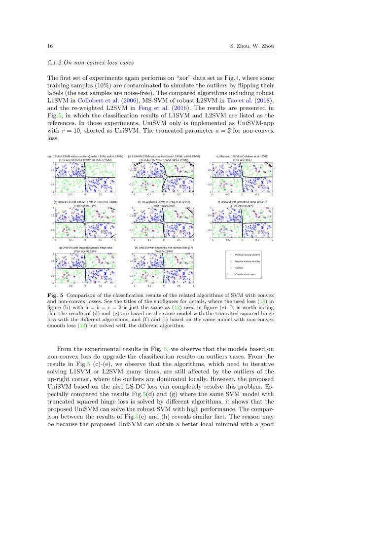
The first set of experiments again performs on “xor” data set as Fig.4, where sometraining samples (10%) are contaminated to simulate the outliers by flipping theirlabels (the test samples are noise-free). The compared algorithms including robustL1SVM in Collobert et al. (2006), MS-SVM of robust L2SVM in Tao et al. (2018),and the re-weighted L2SVM in Feng et al. (2016). The results are presented inFig.5, in which the classification results of L1SVM and L2SVM are listed as thereferences. In those experiments, UniSVM only is implemented as UniSVM-appwith r = 10, shorted as UniSVM. The truncated parameter a = 2 for non-convexloss.
-1 -0.5 0 0.5 1-1
-0.5
0
0.5
1
(a) L1SVM/L2SVM without outliers(dash-L1SVM; solid-L2SVM)(Test Acc:98.25%-L1SVM; 98.75%-L2SVM)
-1 -0.5 0 0.5 1-1
-0.5
0
0.5
1
(b) L1SVM/L2SVM with outliers(dash-L1SVM; solid-L2SVM)(Test Acc:95.75%-L1SVM; 94%-L2SVM)
-1 -0.5 0 0.5 1-1
-0.5
0
0.5
1
(c) Robust L1SVM in Collobert et al. (2006)(Test Acc:98%)
-1 -0.5 0 0.5 1-1
-0.5
0
0.5
1
(d) Robust L2SVM with MS-SVM in Tao et al. (2018)(Test Acc:97.75%)
-1 -0.5 0 0.5 1-1
-0.5
0
0.5
1
(e) Re-wighted L2SVM in Feng et al. (2016)(Test Acc:96.25%)
-1 -0.5 0 0.5 1-1
-0.5
0
0.5
1
(f) UniSVM with smoothed ramp loss (16)(Test Acc:99.25%)
Positive training samples
Negitive training samples
Outliers
Classification curves
-1 -0.5 0 0.5 1-1
-0.5
0
0.5
1
(g) UniSVM with trucated squared hinge loss(Test Acc:99.25%)
-1 -0.5 0 0.5 1-1
-0.5
0
0.5
1
(h) UniSVM with smoothed non-convex loss (17)(Test Acc:99%)
Fig. 5 Comparison of the classification results of the related algorithms of SVM with convexand non-convex losses. See the titles of the subfigures for details, where the used loss (18) infigure (h) with a = b = c = 2 is just the same as (12) used in figure (e). It is worth notingthat the results of (d) and (g) are based on the same model with the truncated squared hingeloss with the different algorithms, and (f) and (i) based on the same model with non-convexsmooth loss (12) but solved with the different algorithm.
From the experimental results in Fig. 5, we observe that the models based onnon-convex loss do upgrade the classification results on outliers cases. From theresults in Fig.5 (c)-(e), we observe that the algorithms, which need to iterativesolving L1SVM or L2SVM many times, are still affected by the outliers of theup-right corner, where the outliers are dominated locally. However, the proposedUniSVM based on the nice LS-DC loss can completely resolve this problem. Es-pecially compared the results Fig.5(d) and (g) where the same SVM model withtruncated squared hinge loss is solved by different algorithms, it shows that theproposed UniSVM can solve the robust SVM with high performance. The compar-ison between the results of Fig.5(e) and (h) reveals similar fact. The reason maybe because the proposed UniSVM can obtain a better local minimal with a good

Unified SVM algorithm based on LS-DC Loss 17
4001000 2000 5000 1000010-3
10-2
10-1
100
101
102
103
(b) Traing time
LibSVM without outliersRobust L1SVM in Collobert et al. (2006)Robust L2SVM with MS-SVM in Tao et al. (2018)Re-wighted L2SVM in Feng et al. (2016)UniSVM with smoothed ramp loss (16)UniSVM with trucated squared hinge lossUniSVM with smoothed non-convex loss (18)LibSVM with outliers
4001000 2000 5000 1000090
91
92
93
94
95
96
97
98
99
100(a) Test accuracies with standard deviations
LibSVM without outliers
Robust L1SVM in Collobert et al. (2006)
Robust L2SVM with MS-SVM in Tao et al. (2018)
Re-wighted L2SVM in Feng et al. (2016)
UniSVM with smoothed ramp loss (16)
UniSVM with trucated squared hinge loss
UniSVM with smoothed non-convex loss (18)
LibSVM with outliers
Fig. 6 The comparisons of the training time and test accuracies (averaged on ten trials) ofthe related algorithms on the contaminated “xor” data sets with different training size.
initial point (a sparse solution of LSSVM) based on the nice DC decomposition ofthe corresponding non-convex loss.
The second set of experiments also compares the effectiveness of the relatedalgorithms on “xor” problem. The training samples are randomly generated withsizes varied from 400 to 10000, and the test samples are generated similarly withthe same sizes. The training data is contaminated by randomly flipping the labels of10% instances to simulate the outliers. We set r = 0.1m for all UniSVM algorithmsto approximate the kernel matrix, and the other parameters are set as the formerexperiments. The corresponding training time and test accuracies (averaged onten trials) of the related robust SVM algorithms are plotted in Fig.6, where theresults of LibSVM (with outliers and without outliers) are also given as references.
From the experimental results in Fig. 6, we have the following findings:
– In Fig. 6(a), it is clear that all related robust SVM algorithms based on non-convex losses do have better test accuracies than those of L1SVM with convexloss very much on the contaminated training data sets, and all of them matchthe results of the noise-free case. At the same time, we notice that the differ-ences between the selected robust algorithms are minimal.
– From Fig. 6(b), we observe that the differences in the training time betweenthe related algorithm are large, especially on the big training set. The trainingtime of the proposed UniSVM is significantly less, while the robust L1SVM(Collobert et al., 2006), Robust L2SVM (Tao et al., 2018) and re-weightedL2SVM (Feng et al., 2016), which need to solve the constrained QP severaltimes, have a long training time. Even they can be more efficiently implemented(such as SMO) than quadprog.m, but their training time will be longer thanthat of LibSVM since all of them at least solve a QP similar to the QP solvedby LibSVM.
– In our setting, the outliers affect the results of LibSVM very much, not onlyon test accuracies but also on training time.
– All in all, the new proposed UniSVM with low-rank kernel approximation isnot only robust to noise but also highly efficient in the training process.
18 S. Zhou, W. Zhou
5.2 Experiments on larger benchmark data sets
This section presents experiments to show that UniSVM can quickly train the con-vex and non-convex SVM models with a comparable performance using a unifiedscheme on large data sets. We only choose state-of-the-arts SVM tool LibSVM(Chang and Lin, 2011)(including SVC and SVR) as the comparator, rather thanother robust SVM algorithms in papers (Collobert et al., 2006; Wu and Liu, 2007;Tao et al., 2018; Feng et al., 2016) to save the experiment time.
Firstly we select 4 classification tasks and 3 regression tasks from the UCIdatabase to illustrate the performance of the related algorithms. The detailedinformation of the data sets and the hyper-parameters (training size, test
size, dimension, λ, γ) are given as follows:Adult: (32561, 16281, 123, 10−5, 2−10), Ijcnn: (43500, 14500, 9, 10−5, 20),
Shuttle: (49990, 91790, 22,10−5, 21), Vechile: (78823, 19705, 100, 10−2, 2−3);Cadata: (10640, 10000, 8, 10−2, 20), 3D-Spatial: (234874, 200000, 3, 10−3, 26),
Slice: (43500, 10000, 385, 10−9, 2−5).
Here the classification tasks have the default splitting, and the regression tasksare split randomly. The λ (regularizer) and γ (for Gaussian kernel κ(x, z) =exp(−γ‖x− z‖2)) are roughly chosen by the grid search. As for the parameters ofloss functions, we use the default value (be given next). Of course, the fine-tuningof all parameters will improve the performance further.
To implement the UniSVM for large training data, we use the pivoted Choleskyfactorization method proposed in Zhou (2016) to approximate the kernel matrixK,and the low-rank approximation error is controlled by the first matched criteriontrace(K − K) < 0.001 ·m or r ≤ 1000, where m is the training size, and r is theupper bound of the rank.
The first set of experiments is to show that the proposed UniSVM can trainSVM models with the convex or non-convex loss for classification problems. Thechosen losses for UniSVM1 to UniSVM10 are listed as following:
UniSVM1: least squares loss, UniSVM2: smoothed hinge (p = 8),UniSVM3: squared hinge loss, UniSVM4: truncated squared hinge (a = 1),UniSVM5: truncated least squares (a = 1), UniSVM6: loss (16) (a = 1),UniSVM7: loss (17) (p = 8), UniSVM8: loss (18) (a = b = c = 2),UniSVM9: loss (18) (a = b = 2, c = 4), UniSVM10: loss (18) (a = 2, b = 3, c = 4).
The results in Table 1 are obtained on the original data sets, and Table 2 onthe contaminated data sets where the labels of training instances are randomlyflipped with a rate of 20%. Since the kernel approximation in Zhou (2016) hasrandom initialization, the training time recorded in Matlab is not very stable, andthere has random flipping for noise cases, all results are averaged over ten randomtrials.
From the results in Table 1 and Table 2, we conclude the following findings:
– UniSVMs with different losses work well using a unified scheme in all cases.In noise-free cases, they are mostly faster than LibSVM with comparable per-formance. The only exception is the result on the lower dimensional data setIjcnn. However, in noise cases, UniSVMs are faster than LibSVM very much.The training time of LibSVM in Table 2 is notable longer than its trainingtime in Table 1 because the flipping process increases a large number of Sup-port Vectors. However, owing to the sparse solution of (28), this influence onUniSVMs is quite weak.

Unified SVM algorithm based on LS-DC Loss 19
Table 1 Classification tasks I–Test accuracies and the training time of the related algo-rithms on the benchmark data sets. All results are averaged over ten trials with the standarddeviations in brackets; The first four lines are based on convex losses, and the others are basedon non-convex losses.
Test accuracy (%) Training time (CPU seconds)
Algorithm Adult Ijcnn Shuttle Vechile Adult Ijcnn Shuttle Vechile
LibSVM 84.65(0.00) 98.40(0.00) 99.81(0.00) 84.40(0.00) 51.49(0.07) 23.02(0.63) 4.75(0.16) 1091(175)UniSVM1 84.56(0.02) 94.65(0.07) 98.80(0.04) 85.24(0.01) 0.44(0.02) 18.24(0.15) 0.34(0.02) 34.77(0.44)UniSVM2 84.68(0.04) 97.07(0.05) 99.81(0.01) 84.42(0.00) 0.98(0.04) 38.51(0.32) 2.44(0.10) 36.66(0.62)UniSVM3 85.13(0.02) 98.22(0.03) 99.82(0.00) 85.23(0.01) 0.62(0.03) 35.40(0.28) 2.03(0.06) 35.34(0.39)
UniSVM4 84.75(0.04) 98.25(0.04) 99.82(0.00) 84.72(0.00) 1.13(0.04) 38.56(0.53) 2.47(0.06) 37.20(0.42)UniSVM5 83.32(0.05) 94.59(0.08) 98.81(0.04) 84.71(0.00) 0.58(0.03) 19.18(0.35) 0.38(0.02) 36.81(0.52)UniSVM6 84.82(0.02) 98.20(0.03) 99.82(0.00) 84.70(0.00) 1.08(0.03) 40.11(0.44) 2.72(0.10) 36.65(0.34)UniSVM7 84.20(0.02) 97.13(0.05) 99.82(0.00) 84.43(0.00) 1.38(0.04) 40.40(0.51) 2.71(0.06) 37.61(0.35)UniSVM8 84.75(0.02) 97.84(0.04) 99.82(0.00) 84.53(0.00) 0.97(0.04) 38.13(0.26) 2.40(0.11) 36.10(0.45)UniSVM9 85.09(0.02) 98.46(0.04) 99.83(0.00) 85.34(0.00) 1.15(0.05) 36.95(0.29) 3.30(0.11) 36.69(0.44)
UniSVM10 85.16(0.03) 98.36(0.03) 99.82(0.00) 85.49(0.00) 0.84(0.03) 33.92(0.22) 2.90(0.15) 36.47(0.55)
Table 2 Classification tasks II–Test accuracies and the training time of the related algo-rithms on the benchmark data sets with flipping 20% labels of training data. All results areaveraged on ten trials with the standard deviations in brackets; The first four lines are basedon convex losses and the others are based on non-convex losses.
Test accuracy (%) Training time (CPU seconds)
Algorithm Adult Ijcnn Shuttle Vechile Adult Ijcnn Shuttle Vechile
LibSVM 78.25(0.00) 93.80(0.00) 98.89(0.00) 84.28(0.04) 104.0(0.8) 191.7(1.2) 82.28(1.52) 1772(123)UniSVM1 84.55(0.02) 93.90(0.08) 98.71(0.04) 85.19(0.00) 0.44(0.06) 18.34(0.33) 0.35(0.02) 34.76(0.43)UniSVM2 82.27(0.06) 93.72(0.04) 99.01(0.10) 84.25(0.00) 0.65(0.07) 20.56(0.39) 0.60(0.04) 36.99(0.43)UniSVM3 84.55(0.02) 93.95(0.08) 98.72(0.04) 85.19(0.00) 0.45(0.06) 18.74(0.34) 0.38(0.02) 34.94(0.44)
UniSVM4 84.26(0.03) 97.36(0.05) 99.81(0.00) 84.37(0.00) 1.23(0.09) 40.23(2.85) 2.52(0.09) 37.53(0.46)UniSVM5 82.62(0.03) 93.96(0.03) 98.81(0.02) 84.34(0.00) 0.60(0.05) 20.25(0.48) 0.39(0.02) 37.50(0.48)UniSVM6 84.25(0.02) 97.59(0.04) 99.81(0.00) 84.46(0.00) 1.14(0.08) 48.74(2.55) 2.72(0.14) 37.19(0.42)UniSVM7 83.80(0.04) 96.05(0.04) 99.67(0.06) 84.28(0.00) 1.52(0.08) 46.14(1.77) 2.67(0.11) 38.14(0.44)UniSVM8 84.38(0.04) 94.76(0.05) 99.25(0.10) 84.39(0.00) 0.76(0.07) 23.32(0.48) 0.99(0.05) 36.53(0.44)UniSVM9 85.09(0.02) 97.68(0.04) 99.80(0.00) 85.31(0.00) 1.06(0.07) 44.67(2.99) 4.29(0.22) 36.55(0.48)
UniSVM10 84.83(0.02) 95.77(0.09) 99.44(0.05) 85.46(0.00) 0.56(0.06) 21.26(0.47) 0.81(0.04) 35.69(0.46)
– Compared with the training time (including the time to obtain P for approx-imating the kernel matrix K) of UniSVM1 (least squares) with others, it isclear the proposed UniSVM has a very low cost after the first iteration, asother UniSVMs always run UniSVM1 in their first iteration.
– All UniSVMs with non-convex loss are working as efficiently as those withconvex loss. Particularly, UniSVMs with non-convex losses maintain high per-formance on the contaminated data sets in Table 2. The new proposed loss(18) with two more parameters always achieves the highest performance.
The second set of experiments is to show the performance of the UniSVM forsolving regression tasks with the convex and non-convex losses. The experimentalresults are listed in Table 3. The chosen losses for UniSVM1 to UniSVM6 are listedas follows:
UniSVM1: least squares loss, UniSVM2: smoothed ε-insensitive loss (20) (p = 100),UniSVM3: Hubber loss (δ = 0.1 ), UniSVM4: smoothed absolute loss (p = 100)UniSVM5: truncated least squares (a = 1), UniSVM6: truncated Hubber loss (δ = 0.1, a = 1).
From the results in Table 3, we again observe that UniSVMs with differentlosses work well by a unified scheme. All of them are more efficient than LibSVMwith comparable performance. For example, LibSVM costs a very long trainingtime on the second task 3D-Spatial, because of too many training samples, and

20 S. Zhou, W. Zhou
Table 3 Regression task–Test RMSE (root-mean-square-error) and the training time of therelated algorithms on the benchmark data sets. All results are averaged over ten trials withthe standard deviations in brackets; The first four lines are based on convex losses, and therest are based on the truncated non-convex losses.
Test RMSE Training time (CUP seconds)
Algorithm Cadata 3D-Spatial Slice Cadata 3D-Spatial Slice
LibSVM 0.314(0.000) 0.464(0.000) — 3.38(0.04) 4165(2166) > 3hrUniSVM1 0.314(0.000) 0.455(0.000) 6.725(0.101) 1.06(0.06) 96.3(5.0) 25.40(0.08)UniSVM2 0.307(0.000) 0.459(0.000) 6.753(0.100) 1.38(0.07) 118.9(4.2) 44.75(1.05)UniSVM3 0.310(0.000) 0.463(0.000) 6.870(0.103) 1.31(0.09) 112.8(3.8) 60.82(1.70)UniSVM4 0.308(0.000) 0.464(0.000) 6.765(0.100) 1.44(0.08) 123.3(4.3) 50.89(1.25)
UniSVM5 0.315(0.000) 0.454(0.000) 6.868(0.116) 1.10(0.06) 99.6(4.1) 83.75(13.30)UniSVM6 0.312(0.000) 0.465(0.000) 6.775(0.105) 1.32(0.07) 121.5(4.9) 75.72(4.45)
LibSVM can not finish the task on the last Slice data set maybe because of toomany Support Vectors. In two cases, all UniSVMs work well with comparableperformance, mainly due to the efficient low-rank approximation of the kernelmatrix. It is also noted that the UniSVMs with non-convex losses are working asefficiently as those with convex loss.
In the third set of experiments, we challenge UniSVM to two classification taskson the very large data sets (up to millions of samples) on the same computer. Theselected data sets are:
– Covtype: It is a binary class problem with 581012 samples and each examplehas 54 features. We randomly split it into 381012 training samples and 200000test samples. The parameters used are γ = 2−2 and λ = 10−8.
– Checkerboard3M: It is based on the noisy free version of 2-dimensional Checker-board data set (4× 4-grid XOR problem), which was widely used to show theeffectiveness of nonlinear kernel methods. The data set was sampled by uni-formly discretizing the regions [0, 1] × [0, 1] to 20002 = 4000000 points andlabeling two classes by 4× 4-grid XOR problem, and was then split randomlyinto 3000000 training samples and 1000000 test samples. The parameters usedare γ = 24 and λ = 10−7.
Those data sets are also used in Zhou (2016). Because of the limited memoryof our computer, the kernel matrix on Covtype is approximated as PP> withP ∈ Rm×1000, and the kernel matrix on Checkerboard3M is approximated PP>
with P ∈ Rm×300, where m is the training size. The experimental results are givenin Table 4, where LibSVM cannot accomplish the tasks because of its long trainingtime. The selected losses are the same as those in Table 1 and Table 2.
From the results in Table 4, we observe that the UniSVM works well on verylarge data sets. We also conclude some similar findings with the results in Table1 and 2. UniSVMs with different losses work well by a unified scheme with com-parable performance, and all the UniSVMs with non-convex loss are working asefficiently as those with convex loss. Particularly, the UniSVMs with non-convexlosses maintain high performance because there may have many contaminatedsamples in very large training cases.
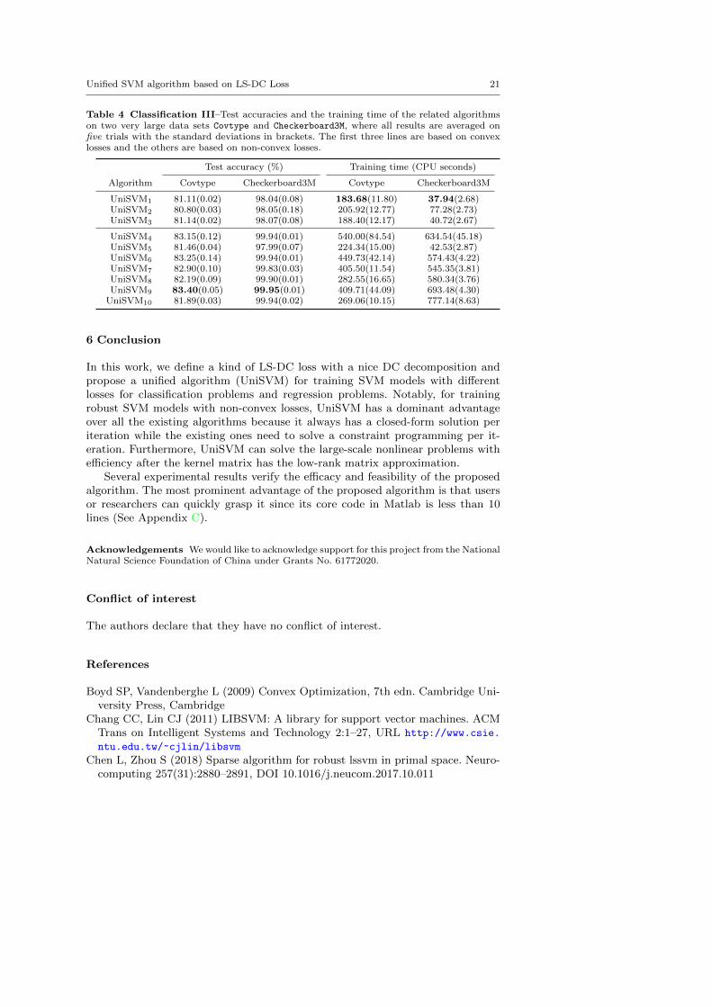
Unified SVM algorithm based on LS-DC Loss 21
Table 4 Classification III–Test accuracies and the training time of the related algorithmson two very large data sets Covtype and Checkerboard3M, where all results are averaged onfive trials with the standard deviations in brackets. The first three lines are based on convexlosses and the others are based on non-convex losses.
Test accuracy (%) Training time (CPU seconds)
Algorithm Covtype Checkerboard3M Covtype Checkerboard3M
UniSVM1 81.11(0.02) 98.04(0.08) 183.68(11.80) 37.94(2.68)UniSVM2 80.80(0.03) 98.05(0.18) 205.92(12.77) 77.28(2.73)UniSVM3 81.14(0.02) 98.07(0.08) 188.40(12.17) 40.72(2.67)
UniSVM4 83.15(0.12) 99.94(0.01) 540.00(84.54) 634.54(45.18)UniSVM5 81.46(0.04) 97.99(0.07) 224.34(15.00) 42.53(2.87)UniSVM6 83.25(0.14) 99.94(0.01) 449.73(42.14) 574.43(4.22)UniSVM7 82.90(0.10) 99.83(0.03) 405.50(11.54) 545.35(3.81)UniSVM8 82.19(0.09) 99.90(0.01) 282.55(16.65) 580.34(3.76)UniSVM9 83.40(0.05) 99.95(0.01) 409.71(44.09) 693.48(4.30)
UniSVM10 81.89(0.03) 99.94(0.02) 269.06(10.15) 777.14(8.63)
6 Conclusion
In this work, we define a kind of LS-DC loss with a nice DC decomposition andpropose a unified algorithm (UniSVM) for training SVM models with differentlosses for classification problems and regression problems. Notably, for trainingrobust SVM models with non-convex losses, UniSVM has a dominant advantageover all the existing algorithms because it always has a closed-form solution periteration while the existing ones need to solve a constraint programming per it-eration. Furthermore, UniSVM can solve the large-scale nonlinear problems withefficiency after the kernel matrix has the low-rank matrix approximation.
Several experimental results verify the efficacy and feasibility of the proposedalgorithm. The most prominent advantage of the proposed algorithm is that usersor researchers can quickly grasp it since its core code in Matlab is less than 10lines (See Appendix C).
Acknowledgements We would like to acknowledge support for this project from the NationalNatural Science Foundation of China under Grants No. 61772020.
Conflict of interest
The authors declare that they have no conflict of interest.
References
Boyd SP, Vandenberghe L (2009) Convex Optimization, 7th edn. Cambridge Uni-versity Press, Cambridge
Chang CC, Lin CJ (2011) LIBSVM: A library for support vector machines. ACMTrans on Intelligent Systems and Technology 2:1–27, URL http://www.csie.
ntu.edu.tw/~cjlin/libsvm
Chen L, Zhou S (2018) Sparse algorithm for robust lssvm in primal space. Neuro-computing 257(31):2880–2891, DOI 10.1016/j.neucom.2017.10.011

22 S. Zhou, W. Zhou
Chen PH, Fan RE, Lin CJ (2006) A study on SMO-type decomposition methodsfor support vector machines. IEEE Transactions on Neural Networks 17(4):893–908
Collobert R, Sinz F, Weston J, Bottou L (2006) Trading convexity for scalabil-ity. In: Proceedings of the 23rd international conference on Machine learning -ICML’06, ACM Press, pp 201–208
Feng Y, Yang Y, Huang X (2016) Robust support vector machines for classificationwith nonconvex and smooth losses. Neural Computation 28(6):1217–1247
Golub GH, Loan CFV (1996) Matrix Computations. The John Hopkins UniversityPress, Baltimore, Maryland
Hampel FR, Ronchetti EM, Rousseeuw PJ, Stahel WA (2011) Robuststatistics:The approach based on influence functions. Hoboken, NJ: Wiley
Jiao L, Bo L, Wang L (2007) Fast sparse approximation for Least Squares SupportVector Machines. Neural Networks, IEEE Transactions on 18(3):685 –697,
Keerthi SS, Shevade SK, Bhattacharyya C, Murthy KRK (2001) Improvements toPlatt’s SMO algorithm for SVM classifier design. Neural Computation 13:637–649
Keerthi SS, Chapelle O, Decoste D (2006) Building Support Vector Machines withreduced classifier complexity. J of Machine Learning Research 7:1493–1515
Naderi S, He K, Aghajani R, Sclaroff S, Felzenszwalb P (2019) Generalizedmajorization-minimization. In: Proceedings of the 36-th International Confer-ence on Machine Learning, Long Beach, CA, USA
Ong CS, Mary X, Canu S, Smola AJ (2004) Learning with non-positive kernels.In: Twenty-first international conference on Machine learning - ICML’04, ACMPress
Platt JC (1999) Fast training of Support Vector Machines using Sequential Min-imal Optimization. In: Scholkopf B, Burges CJ, Smola AJ (eds) Advances inKernel Method-Support Vector Learning, MIT Press, pp 185–208
Rockafellar RT (1972) Convex Analysis, Second Printing. Princeton UniversityPress, Princeton
Scholkopf B, Smola AJ (2002) Learning with Kernels-Support Vector Machines,Regularization, Optimization and Beyond. The MIT Press
Scholkopf B, Herbrich R, Smola AJ (2001) A generalized representer theorem.In: Proceedings of the Annual Conference on Computational Learning Theory,Springer, pp 416–426
Shalev-Shwartz S, Ben-David S (2014) Understanding Machine Learning: FromTheory to Algorithms. Cambridge University Press, New York,
Shen X, Tseng GC, Zhang X, Wong WH (2003) On φ-learning. Journal of theAmerican Statistical Association 98(463):724–734
Steinwart I (2003) Sparseness of Support Vector Machines. Journal of MachineLearning Research 4:1071–1105
Steinwart I, Christmann A (2008) Support Vector Machines. Springer-Verlag, NewYork
Steinwart I, Hush D, Scovel C (2011) Training SVMs without offset. Journal ofMachine Learning Research 12:141–202
Sun S, Zhao J, Zhu J (2015) A review of nystrom methods for large-scale machinelearning. Information Fusion 26:36–48
Suykens J, Vandewalle J (1999a) Least square Support Vector Machine classifiers.Neural Processing Letters 9(3):293–300

Unified SVM algorithm based on LS-DC Loss 23
Suykens JAK, Vandewalle J (1999b) Least squares support vector machine classi-fiers. Neural Processing Letters 9(3):293–300
Suykens JAK, Gestel TV, Brabanter JD, Moor BD, Vandewalle J (2002) Leastsquares Support Vector Machines. World Scientific, River Edge, NJ
Tao PD, Souad EB (1986) Algorithms for solving a class of nonconvex optimiza-tion problems. methods of subgradients. In: Fermat Days 85: Mathematics forOptimization, Elsevier, pp 249–271, DOI 10.1016/s0304-0208(08)72402-2
Tao Q, Wu G, Chu D (2018) Improving sparsity and scalability in regularizednonconvex truncated-loss learning problems. IEEE Transactions on Neural Net-works and Learning Systems 29(7):2782–2793
Thi HAL, Dinh TP (2018) DC programming and DCA: thirty years of develop-ments. Mathematical Programming 169(1):5–68
Vapnik VN (1999) An overview of statistical learning theory. IEEE trans on NeuralNetwork 10(5):988–999
Vapnik VN (2000) The Nature of Statistical Learning Theory. Springer-Verlag,New York
Wu Y, Liu Y (2007) Robust truncated hinge loss support vector machines. Publi-cations of the American Statistical Association 102(479):974–983
Xu HM, Xue H, Chen XH, Wang YY (2017) Solving indefinite kernel supportvector machine with difference of convex functions programming. In: Proceed-ings of the Thirty-First AAAI Conference on Artificial Intelligence, AAAI Press,AAAI’17, pp 2782–2788
Yuille AL, Rangarajan A (2003) The concave-convex procedure. Neural Compu-tation 15(4):915–936
Zhou S (2013) Which is better? Regularization in RKHS vs Rm on Reduced SVMs.Statistics, Optimization and Information Computing 1(1):82–106
Zhou S (2016) Sparse LSSVM in primal using Cholesky factorization for large-scale problems. IEEE Transactions on Neural Networks and Learning Systems27(4):783–795
Zhou S, Liu H, Ye F, Zhou L (2009) A new iterative algorithm training SVM.Optimization Methods and Software 24(6):913–932
Zhou S, Cui J, Ye F, Liu H, Zhu Q (2013) New smoothing SVM algorithm withtight error bound and efficient reduced techniques. Computational Optimizationand Applications 56(3):599–618
Appendix
A The proof of Propositions
A.1 The proof of Propositions 1
Proof We illustrate them one by one.
(a) It is clear.(b) It is because u2 −min{u2, a} = (u2 − a)+ is a convex function.(c) It is because Au2 − u2+ with A ≥ 1 is a convex function.
(d) It is because Au2 −min{u2+, a} = Au2 − u2+ + (u2+ − a)+ with A ≥ 1 is convex.(e) First show that the hinge loss `(y, t) = (1 − yt)+ is not an LS-DC loss. If let g(u) =
Au2 − u+, we have g′−(0) = 0 > g′+(0) = −1. Hence by Theorem 24.1 in Rockafellar
(1972), we conclude that g(u) is not convex for all A (0 < A < +∞).

24 S. Zhou, W. Zhou
Noticed that (1−yt)+ = limp→+∞1p
log(1+exp(p(1−yt))). Let ψ(u) = 1p
log(1+exp(pu)),
and we have ψ′′(u) =p exp(pu)
(1+exp(pu))2≤ p
4. By Theorem 1, we know that `p(y, t) = 1
plog(1 +
exp(p(1 − yt))) is an LS-DC loss with A ≥ p/8. In experiments, letting 1 ≤ p ≤ 100,`p(y, t) is a good approximation of the hinge loss.
(f) The ramp loss is not an LS-DC loss is the same as that of the hinge loss. It’s two smoothedapproximations (16) and (17) are LS-DC loss. The proof of the first is similar to squaredhinge loss, and the proof of the second is similar to the approximated hinge loss.
(g) Let g(u) = Au2 − a(1− exp(− 1
au2+)
). Then g(u) is a convex function because g′(u) =
2Au− 2u+ exp(− 1au2+)) is monotonically increasing if A ≥ 1.
(h) Let ψ(u) = a(1− e−1buc+ ). If c = 2, set A ≥ a
b= 1
2M(a, b, 2) and let g(u) = Au2 − ψ(u).
Hence g(u) is convex because g′(u) = 2Au− 2abu+e
− 1bu2+ is monotonically increasing.
For c > 2, ψ(u) is second-order derivable, according to Theorem 1 we only need to obtainthe upper bound of ψ′′(u). If u ≤ 0, we have ψ′′(u) = 0. If u > 0, then ψ′′(u) =acb
((c− 1)uc−2 − c
bu2c−2
)e−
1buc
and
ψ′′′(u) = acbuc−3e−
1buc(c2
b2u2c − 3c(c−1)
buc + (c− 1)(c− 2)
).
Letting g′′′(u) = 0, we get the roots u∗1 and u∗2 (0 < u∗1 < u∗2), where
u∗1 = (b h(c))1c
with h(c) = (3(c− 1)−√
5c2 − 6c+ 1)/(2c), which is a local maximum of ψ′′(u). Notingthat limu→0 ψ′′(u) = limu→∞ ψ′′(u) = 0, we have that the global maximum of ψ′′(u)reaches at u∗1. Putting u∗1 in ψ′′(u), we prove that ψ′′(u) ≤ M(a, b, c) for any u, where
M(a, b, c) := acb2/c
((c− 1)(h(c))1−2/c − c(h(c))2−2/c
)e−h(c).
For example, M(2, 2, 2) = 2, M(2, 2, 4) ≈ 4.5707 < 5, M(2, 3, 4) ≈ 3.7319 < 4. Thus, theparameter A = 1
2M(a, b, c) is not very large.
A.2 The proof of Propositions 2
Proof We illustrate them one by one.
(1) It is clear.(2) The ε-insensitive loss `ε(y, t) := (|y− t| − ε)+ is not an LS-DC loss. The reason is similar
as that of the hinge loss in item (e). However, its smoothed approximation (20) is LS-DCloss with A ≥ p/4. Actually, let ψ(u) = 1
plog(1+exp(−p(u+ε)))+ 1
plog(1+exp(p(u−ε))).
We have
ψ′′(u) =p exp(−p(u+ ε))
(1 + exp(−p(u+ ε)))2+
p exp(p(u− ε))(1 + exp(p(u− ε)))2
≤p
2.
(3) The absolute loss `(y, t) = |y − t| is also not an LS-DC loss. Clearly, the Hubber loss`δ(y, t) which approximates the absolute loss, is an LS-DC loss with A ≥ 1/(2δ); Settingε = 0 in (20) we obtain another smoothed absolute loss, which is an LS-DC loss withA ≥ p/4.
(4) It is clear.
B The lists of some related losses and their subdifferentials
The most related losses and their subdifferentials for updating γk by (23) are listed in Table5. The LS-DC parameters of the LS-DC losses are also given in last column.In experiments,we always use the lower-bound of the parameter.
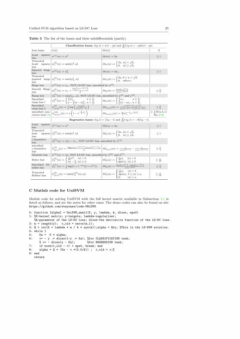
Unified SVM algorithm based on LS-DC Loss 25
Table 5 The list of the losses and their subdifferentials (partly).
Classification losses: `(y, t) = ψ(1− yt) and ∂∂t` (y, t) = −y∂ψ(1− yt).
Loss name ψ(u) ∂ψ(u) A
Least squaresloss
ψ(1)(u) := u2 ∂ψ(u) := 2u ≥ 1
TruncatedLeast squaresloss
ψ(2)a (u) := min{u2, a} ∂ψa(u) :=
{2u, |u| <
√a,
0, |u| ≥√a,
Squared hingeloss
ψ(3)(u) := u2+ ∂ψ(u) := 2u+ ≥ 1
Truncatedsquared hingeloss
ψ(4)a (u) := min{u2+, a} ∂ψa(u) :=
{2u, 0 < u <
√a,
0, others,
Hinge loss ψ(5)(u) := u+, NOT LS-DC loss, smoothed by ψ(6).
Smooth Hingeloss
ψ(6)p (u) := u+ +
log(1+e−p|u|
)p
∂ψp(u) :=min{1,epu}(1+e−p|u|) ≥ p
8
Ramp loss ψ(7)a (u) := min{u+, a}, NOT LS-DC loss, smoothed by ψ(8) and ψ(9).
Smoothedramp loss 1
ψ(8)a (u) :=
{ 2au2+, u ≤ a
2,
a− 2a
(a− u)2+, u >a2,
∂ψa(u) :=
{ 4au+, u ≤ a
2,
4a
(a− u)+, u >a2,
Smoothedramp loss 2
ψ(9)(a,p)
(u) := 1p
log(
1+epu
1+ep(u−a)
)∂ψ(a,p)(u) := e−p(u−a)−e−pu
(1+e−p(u−a))(1+e−pu)≥ p
8
smoothed non-convex loss(18)
ψ(10)(a,b,c)
(u) := a
(1− e−
1buc+
)∂ψ(a,b,c)(u) := ac
buc−1+ e−
1buc+
≥ 12M(a, b, c)
See (19)
Regression losses: `(y, t) = ψ(y − t) and ∂∂t` (y, t) = −∂ψ(y − t).
Least squaresloss
ψ(1)(u) := u2 ∂ψ(u) := 2u ≥ 1
Truncatedleast squaresloss
ψ(2)a (u) := min{u2, a} ∂ψa(u) :=
{2u, |u| <
√a,
0, |u| ≥√a,
≥ 1
ε-insensitiveloss
ψ(3)ε (u) := (|u| − ε)+, NOT LS-DC loss, smoothed by ψ(4).
smoothedε-insensitiveloss
ψ(4)(p,ε)
(u) :=log((1+e−p(u+ε))(1+ep(u−ε)))
p∂ψ(p,ε)(u) := 1
1+ep(u−ε) −1
1+e−p(ε+u) ≥ p4
Absolute loss ψ(5)(u) := |u|, NOT LS-DC loss, smoothed by ψ(6) and ψ(7).
Huber loss ψ(6)δ (u) :=
{ 12δu2, |u| < δ,
|u| − δ2, |u| ≥ δ, ∂ψδ(u) :=
{12δu, |u| < δ,
sgn(u), |u| ≥ δ, ≥ 12δ
Smoothed Ab-solute loss
ψ(7)p (u) := 1
plog((1 + e−pu)(1 + epu)) ∂ψp(u) :=
min{1,epu}−min{1,e−pu}1+e−p|u| ≥ p
4
TruncatedHubber loss
ψ(8)(δ,a)
(u) := min{ψ(6)δ (u), a} ∂ψδ(u) :=
12δu, |u| < δ,
sgn(u), δ ≤ |u| ≤ a,0, |u| > a.
≥ 12δ
C Matlab code for UniSVM
Matlab code for solving UniSVM with the full kernel matrix available in Subsection 4.1 islisted as follows, and see the notes for other cases. The demo codes can also be found on sitehttps://github.com/stayones/code-UNiSVM.
0: function [alpha] = UniSVM_small(K, y, lambda, A, dloss, eps0)1: %K-kernel matrix; y-targets; lambda-regularizer;
%A-parameter of the LS-DC loss; dloss-the derivative function of the LS-DC loss.2: m = length(y); v_old = zeros(m,1);3: Q = inv(K + lambda * m / A * eye(m));alpha = Q*y; %This is the LS-SVM solution.4: while 15: Ka = K * alpha;6: v= - y .* dloss(1-y .* Ka); %for CLASSIFICATION task;
% v= - dloss(y - Ka); %for REGRESSION task;7: if norm(v_old - v) < eps0, break; end8: alpha = Q * (Ka - v *(0.5/A)) ; v_old = v;%9: end
return

26 S. Zhou, W. Zhou
Note:1) With squared hinge loss, dloss(u)=2*max(u,0);
With truncated squared hinge loss, dloss(u)=2*max(u,0).*(u<=sqrt(a));With truncated least squares loss, dloss(u)=2*(u).*(abs(u)<=sqrt(a));With other losses, dloss(u) given in the Table 5 in Appendix B.
2) For large training problem, the input K is taken place as P and B with K=P*P’,then make the following revisions:Line 3 --> Q=inv((lambda*m/A*eye(length(B)) + P’*P)*P(B,:)’);alpha = Q*(P’*y);Line 5 --> Ka = P*(P(B,:)’*alpha);Line 8 --> alpha = Q*(P’*(Ka - v *(0.5/A))); v_old = v.