Embed Size (px)
Citation preview

Comments welcome.
Unequal Opportunities and Human Capital Formation
Daniel Mejía and Marc St-Pierre1
This Version: August 2004
Abstract
This paper develops a tractable, heterogeneous agents general equilibriummodel
where individuals have different endowments of the factors that complement the
schooling process. The paper explores the relation between inequality of oppor-
tunities, inequality of outcomes, and efficiency in human capital formation. Using
numerical solutions we study how the endogenous variables of the model respond to
two different interventions in the distribution of opportunities: a mean-preserving
spread and a change in the support of the distribution of endowments. The re-
sults from the simulation of the model suggest that a higher degree of inequality of
opportunities is associated with lower average human capital in the population, a
lower fraction of individuals investing in human capital, higher inequality in the dis-
tribution of human capital, and higher wage inequality. In other words, the model
(based on standard assumptions) does not predict a trade-off between efficiency and
equality of opportunity in human capital formation.
Keywords: Human Capital, Inequality, Equity-Efficiency Trade-off.
JEL Classification Numbers: J24, J31, O15, D33.1The authors wish to thank Sean Campbell, Adriana Camacho, Pedro Dal Bó, Oded Ga-
lor, Herschel Grossman, Alaka Holla, Peter Howitt, Tom Krebs, Herakles Polemarchakis, Car-los Esteban Posada, as well as participants at the Macro Lunch at Brown U., and LAMES2004 in Santiago for helpful comments and suggestions. However, the remaining errors arethe authors’ responsibility. D. Mejía: Brown University and Banco de la República, Colom-bia. E-mail: [email protected]. M. St-Pierre: Brown University. E-mail: [email protected]. The first author aknowledges financial support from the Tinker Field Re-search Grant.
1. Introduction
The importance of human capital accumulation as an engine of economic growth and
development has been widely recognized in theoretical and empirical studies.2
Most of the literature that studies the effects of income inequality on economic
growth through its effects on human capital accumulation has focused on the role of
credit constraints. The main idea of this line of research is the following: relatively poor
individuals don’t have the means to finance the accumulation of human capital, and,
because they are credit constrained (that is, there is no way to finance the costs of human
capital accumulation using future earnings as the collateral for a loan to pay the tuition
fees and living expenses), they end up either not investing in human capital or investing
very little. Furthermore, if in addition to credit constraints there are decreasing returns
to the accumulation of human capital, the final outcome does not maximize the size of
the economic pie. Consequently there may be space for redistribution of resources from
rich to poor individuals which, in turn, increases the size of the pie. This redistribution
would reallocate resources towards more profitable investments given that the marginal
returns to human capital accumulation are higher for those individuals (the relatively
poor ones) who have less human capital. The theoretical idea has been extensively
developed in the literature since the work by Galor and Zeira (1993) and Banerjee and
Newman (1993). Further developments have been proposed by De Gregorio (1996) and
Bénabou (1996, 2000).3 Empirical evidence has been found in favor of the hypothesis
that inequality and credit constraints affect investment in human capital by Flug et al.
(1998), De Gregorio (1996) and Mejía (2003).
But the accumulation of human capital involves other complementary factors as
well. This has been extensively documented in a number of recent empirical studies,
some of which will be reviewed in the next section. While some of these complemen-
tary factors can be thought of as non-purchasable (neighborhood effects shaped by2The reader is referred to the seminal contributions of Lucas (1988) on the theoretical side, and
those of Mankiw, Romer and Weil (1992), Benhabib and Spiegel (1994, 2003) and Barro (2001) for
the empirical evidence supporting the importance of human capital in explaining growth rates across
countries.3See Aghion et al. (1999) for a thorough review of this literature.
2

local communities, family background, socioeconomic characteristics, genes, provision
of social connections, installation of preferences and aspirations in children), others are
(pre and post natal care, parental level of education, distance to schools and different
qualities of books, teachers and schools).4
If the previously mentioned factors are important in determining differences in ed-
ucational attainment across individuals, the distribution of these “socio-economic char-
acteristics” across individuals matters. In other words, if the distribution of access to
the schooling system is important, one should encounter differences in educational at-
tainment across individuals even in economies with universally free public schools. This
does not rule out the importance of the lack of financial resources to pay for the (mone-
tary) costs of education.5 As said before, different studies have shown that they are, in
fact, important. However, this paper focuses on a complementary explanation, namely,
on the effects of inequality of endowments of the complementary factors to the schooling
system on human capital accumulation decisions made by individuals. More precisely,
the paper explores another explanation for the negative relation between economic in-
equality and the average amount of human capital based on differences in the rates of
return to time investment in human capital accumulation, the latter being determined
by each individual’s endowment of the complementary factors to the schooling system.
The model addresses the relationships between inequality of opportunities, efficiency
in human capital formation, and inequality of outcomes in a general equilibrium frame-
work. This paper is related to the literature that links economic inequality and human
capital accumulation and stresses the negative relation between these two variables (see,
among others, Galor and Zeira, 1993, and Bénabou, 1996, 2000a, 2000b).
The paper is organized as follows: the second section presents the stylized facts
that motivate the construction of the model. Namely, the negative relation between the
degree of inequality in the distribution of human capital and the average level of human
capital across countries, and the positive relation between inequality of opportunities4See Schultz (1988), Roemer (2000), Bénabou (2000), Carneiro and Heckman (2002) and Dardanoni
et al. (2003), among others.5 In fact, family income has been found to have large explanatory power on longitudinal studies of
educational outcomes across individuals.
3

and inequality of outcomes. Also, this section reviews the empirical evidence regarding
the importance of the complementary factors to the schooling system on educational
outcomes, on which the model is based. The third section presents the model, and the
fourth section the results of the model’s numerical solution using a distribution function
that allows us to simulate different degrees of inequality of opportunity, while keeping the
mean of the distribution constant. The last section presents some concluding remarks.
2. Stylized Facts
2.1. The Macro Picture
The main focus of this paper has to do with the relationship between the degree of
inequality in the distribution of the complementary factors to the schooling system
across individuals and the average level of human capital. Although we do not have
a direct measure of the degree of inequality in the distribution of the complementary
factors to the schooling process across countries, we do know from a recent paper by
Thomas et. al (2002) that the human capital Gini coefficient and the average years
of schooling among the adult population are negatively associated in the cross country
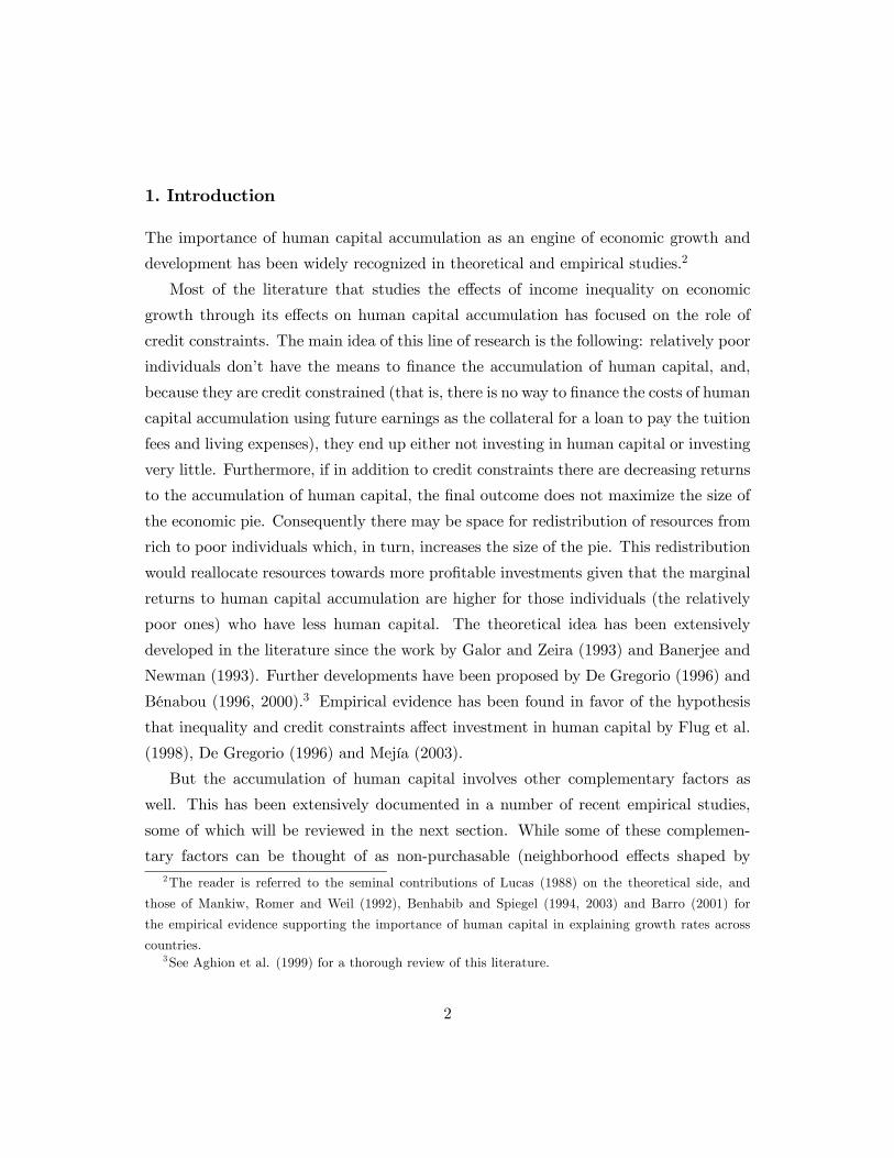
data (see Figure 2.1, taken from Thomas et. al, 2002).6
Those countries with the highest degree of inequality in the distribution of human
capital (as measured by the human capital Gini coefficient) have the lowest average
years of schooling across the adult population.
Some papers have argued that the relationship between inequality in the distribution
of human capital and average human capital follows a “Kuznetian” curve. In other
words, inequality in the distribution of human capital first increases with average human
capital and then declines. However, this relation is observed only when the standard
deviation of schooling is used as a measure of inequality (see Thomas et. al, 2002 for a
review of the evidence, and the main problems associated with the use of the standard
deviation as a measure of human capital inequality).6The authors show that the relation between human capital inequality and average human capital
follows the same pattern if the Theil Index is used as the measure of human capital inequality.
4

Source: Thomas et al. (2000)
Average years of schooling and Education Gini
0
2
4
6
8
10
12
14
0.0000 0.2000 0.4000 0.6000 0.8000 1.0000
Education Gini
Avg
. yea
rs o
f sch
oolin
g (p
op. o
f age
15
and
over
Figure 2.1: Average Human Capital and Human Capital Inequality
2.2. The Micro Evidence on the Importance of the Complementary Factors
to the Educational Process
Since the publication of the Coleman Report (Coleman et al., 1966), hundreds of pa-
pers have studied the relationship between school expenditure and the complemen-
tary factors to the schooling process on different measures of educational outcomes in
the United States. More precisely, the Coleman Report found that the socioeconomic
composition of the student body had a significant effect on test scores after control-
ling for student background, school and teacher characteristics (Ginther et al., 2000).
These findings attracted the attention of scholars and policy makers, as one of its main
conclusions was that school characteristics were relatively unimportant in determining
achievement, while family characteristics were the main determinant of student success
or failure (Hanushek, 1996). Since then, many studies have used different data sets and
5

econometric techniques to improve the estimates of the effects of family background,
parental education, neighborhood effects and many other socioeconomic characteristics
on educational outcomes.7
In a study with more than 5,000 undergraduates at UC San Diego, Betts and Morell
(1997) found that personal background (family income and race) and the demographic
characteristics of former high school classmates, significantly affected students’ GPAs.
This result was obtained after controlling for the degree program in which the stu-
dents were enrolled and the resources of the high school attended. Moreover, they
found that school characteristics partially reflected the incidence of poverty and the
educational level among adults in students’ high-school neighborhood. Goldhaber and
Brewer (1997) found that family background characteristics had a significant effect on
test scores achieved by 18,000 students in the 10th grade, even after controlling for
school characteristics and the results of a previously taken math test by the same stu-
dents. They found that, for instance, years of parental education and family income
were positively related to test scores. Also, black or Hispanic children, and children with
no mother in the household had, on average, a lower predicted score in the math test. A
study by Groger (1997) found empirical evidence of the negative (and significant) effects
of local violence on the likelihood of graduating from high school. While the average
dropout rate in his sample was 21 percent, minor violence increased the dropout rate by
5 percentage points, moderate levels of violence raised it by 24 percent, and substantial
violence by 27 percent.
Data requirements for longitudinal studies constitute the main constraint in esti-
mating the effects of the complementary factors to the schooling process on educational
outcomes in developing countries. However, the use of randomized experiments to es-
timate the effects of changes in the complementary factors (such as improving health
conditions, providing educational inputs, and lowering the costs associated with school
attendance) on different measures of educational outcomes has become one of the most7For a review of the literature, as well as the main findings (and econometric specification problems)
the reader is refered to Ginther et al. (2000) and Hanushek (1986 and 1996). The paper by Durlauf
(2002) presents a complete review of how social interactions play an important role on the perpetuation
of poverty, although not only through the human capital channel.
6
popular topics in the recent development literature.8 The list of recent papers that eval-
uate the effects of improving the accessibility of these complementary factors is growing
rapidly, but a thorough survey of their findings is not the purpose of this article. Some
examples, however, are worth mentioning.
One of these randomized experiments evaluates the effects of mass deworming in
seventy five school populations in Kenya. The results are clear: “Health and school
participation improved not only at program schools, but also at nearby schools, due
to reduced disease transmission. Absenteeism in treatment schools was 25% (or 7 per-
centage points) lower than in comparison schools. Including this spill-over effect, the
program increased schooling by 0.15 years per person treated” (Kremer and Miguel,
2001). The same pattern of results was found in a similar randomized experiment in
India (see Bobonis et al., 2002).
In another randomized experiment conducted in Colombia, vouchers to cover more
than half of the tuition costs of secondary education in private schools were distributed
by lottery to children of secondary school age from neighborhoods classified as falling
into the two lowest socioeconomic strata.9 The effects of this program were estimated
by Angrist et al. (2003) by measuring the differences in certain characteristics and test
scores between voucher winners and a control group of nonparticipants in the program.
After three years in the program, voucher winners were 15 percentage points more
likely to have attended a private school, were 10% more likely to have completed the
8th grade, and scored 0.2 standard deviations higher on standardized tests given to
the whole population (voucher winners plus a control group of nonparticipants in the
program).10
Handa (2002) shows that building more schools and raising adult literacy have a8The reader is referred to Duflo and Kremer (2003) and Kremer (2003) for a review of the method-
ology of randomized experiments as well as their main findings.9Neighborhoods in Colombia are stratified from 1 (the poorest) to 6 (the richest), mainly for purposes
of setting utilities tariffs in a progressive manner.10Other randomized experiments include: PROGRESA in Mexico (Schultz, forthcoming), school
meals in Kenya (Kremer and Vermeersch, 2002), provision of uniforms, textbooks and classroom con-
struction in Kenya (Kremer et al., 2002), provision of a second teacher (if possible, female) in one-teacher
schools in India (Banerjee and Kremer, 2002).
7

larger impact on enrollment rates in primary school in Mozambique than interventions
that raised household income. Also, different dimensions of school quality (such as the
number of trained teachers) and access to school have a positive and significant impact
on school enrollment rates.
A recent paper by Bourguignon et al. (2003) studies the relationship between in-
equality of opportunities in human capital formation and earnings inequality in Brazil.
According to the authors, parental schooling level explains between 35 and 47 percent
of children’s schooling. This paper also finds that inequality of opportunities (that is,
individual circumstances such as parental levels of education, parental occupation, race
and region of origin) accounts for 8-10 percentage points of earnings inequality. Accord-
ing to the authors, between half and three fourths of this share can be attributed to
parental schooling level alone.
In the following section we will construct a tractable general equilibrium model
with heterogeneous agents that accounts for some of the stylized facts described in this
section. Namely, for the negative relation between the average level of human capital in
the economy and the degree of inequality in the distribution of human capital, and for
the positive relation between the degree of inequality of opportunities and the degree
of inequality of outcomes (human capital and wage distribution).
3. The Model
Consider an economy operating under perfectly competitive markets. The production of
the (single) final good is determined by a neoclassical production function that combines
physical capital, human capital and unskilled labor.
Individuals are identical regarding their preferences and cognitive abilities, but may
differ on their endowments of the complementary factors to the schooling process. Each
individual’s endowment of the complementary factors can be thought of as a composite
index of parental level of education, child nourishment, neighborhood and peer effects,
and the degree of accessibility to the formal schooling system, among other things. The
distribution of the complementary factors to the schooling process across individuals is
assumed to be exogenously given, and we will refer to the degree of inequality in this
8

distribution as the degree of “inequality of opportunities”. Given her endowment of
the complementary factors, each individual in the economy decides how much time she
would invest in human capital formation (if any), and then compares the income she
would receive if she decides to work as a skilled worker, with the wage she would receive
if she decides not to invest time in human capital formation and to work as an unskilled
worker.
Although unequal access to the complementary factors of the educational system
can be partially linked to wealth or income inequality, there are some predetermined
characteristics of individuals that cannot be modified and/or cannot be purchased in
the market once the time to make investment decisions in education comes, e.g. pre-
and post-natal care, neighborhood effects, parental level of education and school quality.
In order to concentrate on the effects of inequality of opportunities on human capital
investment decisions, it will be assumed that all individuals are endowed with an equal
share of the total capital stock of the economy and the production of human capital uses
only the individual’s time. In other words, we will assume that investment in human
capital does not involve any monetary payment, and as a result our explanation for the
negative relation between human capital and inequality will not rely on the existence
of credit market imperfections to finance educational investments as in Galor and Zeira
(1993). However, it will be assumed that the amount of time of labor force partici-
pation that an individual sacrifices per unit of time invested in education varies with
the individual’s endowment of the complementary factors to the educational process.
Summarizing the previous ideas, our model explores another explanation for the neg-
ative relation between average human capital and human capital inequality based on
differences in the rates of return to time investment in human capital. The latter, in
turn, are determined by each individual’s endowment of the complementary factors to
the schooling process.
3.1. Production Technology and Firms’ Optimization Conditions
The technology of production of the final good combines unskilled labor, skilled labor
(human capital) and physical capital according to a neoclassical production function
9

characterized by aggregate constant returns to scale and diminishing marginal returns
to each one of these factors (equation 3.1).
Y = F (Lu,H,K) = (Lu)αHβK1−α−β, (3.1)
where Lu is the number of individuals who work as unskilled labor; H is total human
capital in the economy, given by H = Ls_hs, with Ls being the number of individuals
that acquire human capital and_hsbeing the average level of human capital across
those individuals who invest a positive amount of their time in human capital formation
and work as skilled workers; K is the aggregate capital stock, which is assumed to be
exogenously given and equally distributed across individuals.11 For the sake of simplicity
it is assumed that the total population consists of a continuum of individuals of size 1.
That is, it will be assumed that: Lu + Ls = 1.
Markets are assumed to be perfectly competitive and firms choose the number of
unskilled and skilled workers they hire as well as physical capital in order to maximize
profits. The inverse demand for each one of the factors of production is given by
equations 3.2 to 3.4.
wu = α(Lu)α−1HβK1−α−β (3.2)
ws = β (Lu)αHβ−1K1−α−β (3.3)
r = (1− α− β) (Lu)αHβK−α−β (3.4)
Where wu is the unskilled wage rate, ws is the wage rate per unit of human capital,
and r is the rental rate of capital.11A plausible extension of the model would be to assume that each individual’s share of the total
capital stock determines her endowment of the complementary factors to the schooling process. As will
become apparent later on, we conjecture that this extension will only make stronger the results obtained
in the paper.
10

3.2. Individual’s Human Capital Decision
Individuals are identical in their preferences and cognitive abilities and each of them
is endowed with one unit of time which they allocate between labor force participation
and investment in human capital (if any). The fraction of time allocated by individual
i to the accumulation of human capital will be denoted by ui, where 0 ≤ ui < 1.
Also, we will assume that for each unit of time, ui, that individual i devotes to human
capital accumulation, she will acquire a level of human capital equal to b(ui). In words,
human capital formation uses only individuals’ time, and the function b(u) captures the
technology of human capital formation. It will be assumed that b(u) is an increasing
and concave function of the fraction of time invested in human capital formation, u.
That is, b0(u) > 0 and b00(u) < 0. For the sake of simplicity we will use the following
functional form for the technology of human capital formation:
b(ui) = uγi with 0 < γ < 1, (3.5)
where γ measures the elasticity of human capital with respect to time devoted to its
accumulation.
In addition to an endowment of one unit of time, each individual in the economy has
a given endowment of the complementary factors to the educational process. We will
denote individual i’s endowment of the complementary factors by θi, where θi ≥ 0.12Furthermore, it will be assumed that θi is distributed across individuals according to
the distribution function F (θ,φ), that is θ ∼ F (θ,φ), with the support of θ being: [θ, θ],and θ ≥ 0. The parameter φ will be used later to capture the degree of equality in
the distribution of endowments of the complementary factors to the schooling process
across individuals.
Each individual i’s endowment of the complementary factors to the schooling process,
θi, determines the effective time cost (in terms of labor force participation) per unit of
time devoted to human capital formation.13 This idea will be introduced in the model12For instance, θi can be thought of as a composite index of different complementary factors to the
schooling process, such as parental level of education and health (see footnote 16 and Appendix A1).13Note that the endowment θi determines individual i0s rate of return of time investment in human
capital accumulation.
11

in, perhaps, the simplest way: for each unit of time that individual i allocates to the ac-
cumulation of human capital, she sacrifices a fraction of time of labor force participation
equal to1
1 + θi. As discussed in the introduction, this assumption captures the idea
that different individuals face different costs of acquiring human capital. Note that the
larger the endowment of the complementary factor that individual i has, the lower the
fraction of time of labor force participation that she sacrifices per unit of time invested
in the formation of human capital.
The total effective time of labor force participation sacrificed by an individual i, who
invests a fraction ui of her time in human capital accumulation, is given by:ui
1 + θi. The
remaining fraction of time, 1− ui1 + θi
, is devoted to (skilled) labor force participation.
Summarizing, individual i’s supply of human capital in the labor market is given by:
hi = (1− ui1 + θi
)uγi , (3.6)
where the term in parenthesis in the right hand side of equation 3.6 is the amount of
time devoted to (skilled) labor force participation, and the second term is the amount
of human capital acquired by individual i.
Each individual in the economy takes the skilled wage rate, ws, as given, and chooses
the fraction of time investment in human capital accumulation, ui, in order to maximize
her total wage income. That is, each individual i solves the following problem:
maxui
wshi = maxui
ws(1− ui1 + θi
)uγi (3.7)
subject to: 0 ≤ ui ≤ 1
The solution to the above constrained maximization problem is given by:14
u∗i =γ
(1 + γ)(1 + θi) (3.8)
14We will assume throughout that_
θ <1
γ, and therefore the second order condition that guarantees
that the solution found is a global maximum is satisfied for all individuals.
12

Not surprisingly, the higher the endowment of complementary factors to the school-
ing system for individual i is, the larger is her time investment in human capital forma-
tion.15
Replacing the result obtained in equation 3.8 into equation 3.6, individual i’s supply
of human capital in the labor market is given by:
h(θi) =γγ
(1 + γ)1+γ(1 + θi)
γ (3.9)
The higher individual i’s endowments of the complementary factors to the schooling
system is, the greater is her supply of human capital in the labor market.
3.3. Occupational Choice
Given individual i’s endowment of the complementary factors, and the corresponding
optimal time investment in human capital accumulation derived in the previous subsec-
tion (equation 3.8), she compares the income she would receive under the two alternative
occupations: skilled or unskilled.
On the one hand, she can become an unskilled worker, which implies no time in-
vestment in human capital formation. Under this alternative she would supply one unit
of unskilled labor in the market and her income would be given by the unskilled wage
rate. That is:
Income of an unskilled worker = wu (3.10)
On the other hand, if she decides to become a skilled worker, she would optimally
invest a fraction u∗i of her time in the accumulation of human capital, and her total
wage income would be given by the skilled wage rate multiplied by the amount of
human capital she supplies in the labor market (as given by equation 3.9). That is:
Income of skilled worker i= wsγγ
(1 + γ)1+γ(1 + θi)
γ (3.11)
15Note that from the optimization conditions an econometric specification can be derived if the re-
searcher has some hypothesis about the factors that determine θi (see the Appendix (A1) for an exam-
ple).
13

Individual i chooses the occupation that yields the highest income. Comparing the
incomes under the two alternative occupations (expressions 3.10 and 3.11), there exists
a threshold value of the endowment, which we will denote by θ∗, that determines which
individuals decide to invest in human capital and work as skilled workers, and which
individuals decide to devote no time to human capital formation and work as unskilled
workers. In other words, those individuals with an endowment θi = θ∗ are indifferent
between investing a fraction of time u∗i in human capital formation and working as
skilled workers, and devoting all their time to working as unskilled workers. Equating
the two alternative incomes given in expressions 3.10 and 3.11, the threshold endowment
of the complementary factors to the schooling process is given by:
θ∗ =µ(1 + γ)1+γ
γγwu
ws
¶1/γ− 1 (3.12)
Those individuals who have an endowment lower than the threshold endowment θ∗
will not invest any time in human capital formation and will work as unskilled labor,
whereas those individuals with an endowment of the complementary factors larger than
the threshold endowment will invest a fraction u∗i (equation 3.8) of their time in human
capital formation and will work as skilled labor.16 The optimal occupational choice by
individual i is summarized by the following two expressions:
If θi < θ∗ ⇒ Work as unskilled worker and receive income = wu (3.13)
If θi ≥ θ∗ ⇒ Invest u∗i in the acquisition of human capital,
work as skilled worker and receive income = wsγγ
(1 + γ)1+γ(1 + θi)
γ
(3.14)
Given the occupational choice of each individual, and the assumption that the en-
dowments of the complementary factors to the schooling process are distributed across16This result follows from the fact that the income of skilled workers increases in θ (equation 3.11).
14
the population according to the distribution function F (θ,φ), the number of unskilled
individuals, Lu, is given by the fraction of the population with an endowment of the
complementary factors lower than the threshold endowment. Similarly, the number of
skilled individuals, Ls, is given by the fraction of individuals with an endowment of
the complementary factors larger than the threshold endowment. Summarizing, the
numbers of unskilled and skilled individuals are given by the following expression:
Lu = F (θ∗,φ) and Ls = 1− F (θ∗,φ), (3.15)
where F (θ∗,φ) is the fraction of individuals with an endowment of the complemen-
tary factors lower than the threshold endowment.
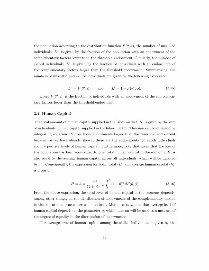
3.4. Human Capital
The total amount of human capital supplied in the labor market, H, is given by the sum
of individuals’ human capital supplied in the labor market. This sum can be obtained by
integrating equation 3.9 over those endowments larger than the threshold endowment
because, as we have already shown, these are the endowments for which individuals
acquire positive levels of human capital. Furthermore, note that given that the size of
the population has been normalized to one, total human capital in the economy, H, is
also equal to the average human capital across all individuals, which will be denoted
by:_h. Consequently, the expression for both, total (H) and average human capital (
_h),
is given by:
H =_h =
γγ
(1 + γ)1+γ
Z _θ
θ∗(1 + θ)γ dF (θ,φ) (3.16)
From the above expression, the total level of human capital in the economy depends,
among other things, on the distribution of endowments of the complementary factors
to the educational process across individuals. More precisely, note that average level of
human capital depends on the parameter φ, which later on will be used as a measure of
the degree of equality in the distribution of endowments.
The average level of human capital among the skilled individuals is given by the
15
total human capital in the economy (equation 3.16) divided by the number of skilled
individuals. That is, average human capital among the skilled individuals is given by:
_hs=
γγ
(1 + γ)1+γ
Z _θ
θ∗(1 + θ)γ dF (θ,φ)
1− F (θ∗,φ) (3.17)
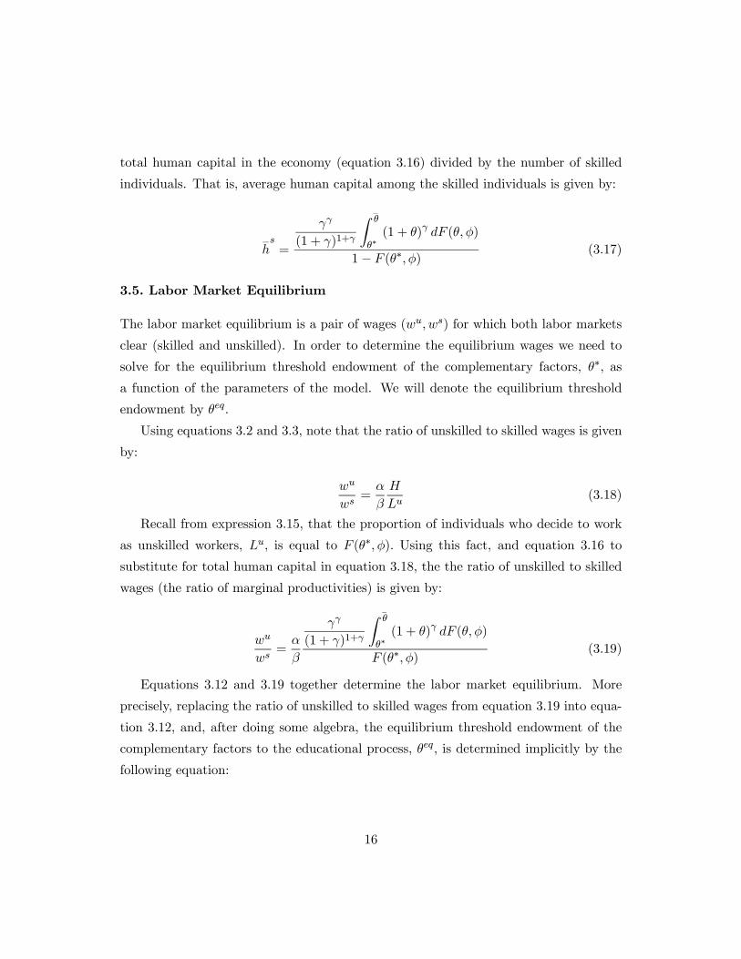
3.5. Labor Market Equilibrium
The labor market equilibrium is a pair of wages (wu, ws) for which both labor markets
clear (skilled and unskilled). In order to determine the equilibrium wages we need to
solve for the equilibrium threshold endowment of the complementary factors, θ∗, as
a function of the parameters of the model. We will denote the equilibrium threshold
endowment by θeq.
Using equations 3.2 and 3.3, note that the ratio of unskilled to skilled wages is given
by:
wu
ws=
α
β
H
Lu(3.18)
Recall from expression 3.15, that the proportion of individuals who decide to work
as unskilled workers, Lu, is equal to F (θ∗,φ). Using this fact, and equation 3.16 to
substitute for total human capital in equation 3.18, the the ratio of unskilled to skilled
wages (the ratio of marginal productivities) is given by:
wu
ws=
α
β
γγ
(1 + γ)1+γ
Z _θ
θ∗(1 + θ)γ dF (θ,φ)
F (θ∗,φ)(3.19)
Equations 3.12 and 3.19 together determine the labor market equilibrium. More
precisely, replacing the ratio of unskilled to skilled wages from equation 3.19 into equa-
tion 3.12, and, after doing some algebra, the equilibrium threshold endowment of the
complementary factors to the educational process, θeq, is determined implicitly by the
following equation:
16
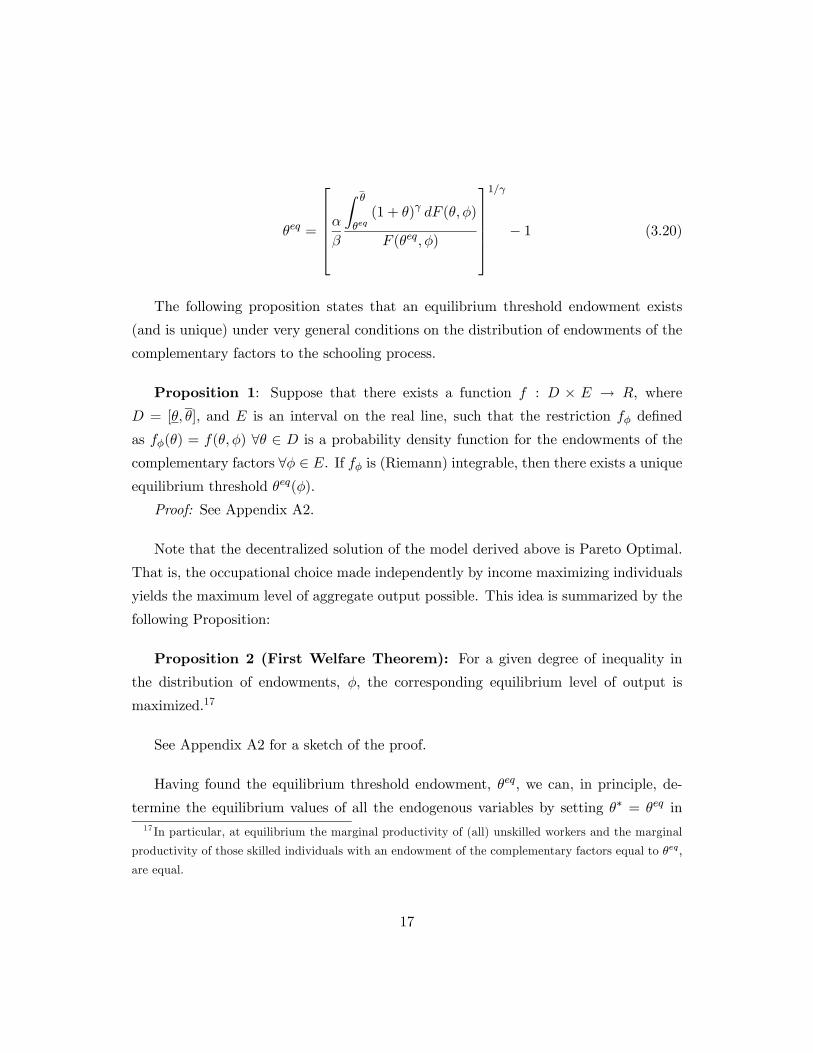
θeq =
⎡⎢⎢⎢⎢⎣αβZ _
θ
θeq(1 + θ)γ dF (θ,φ)
F (θeq,φ)
⎤⎥⎥⎥⎥⎦1/γ
− 1 (3.20)
The following proposition states that an equilibrium threshold endowment exists
(and is unique) under very general conditions on the distribution of endowments of the
complementary factors to the schooling process.
Proposition 1: Suppose that there exists a function f : D × E → R, where
D = [θ, θ], and E is an interval on the real line, such that the restriction fφ defined
as fφ(θ) = f(θ,φ) ∀θ ∈ D is a probability density function for the endowments of the
complementary factors ∀φ ∈ E. If fφ is (Riemann) integrable, then there exists a uniqueequilibrium threshold θeq(φ).
Proof: See Appendix A2.
Note that the decentralized solution of the model derived above is Pareto Optimal.
That is, the occupational choice made independently by income maximizing individuals
yields the maximum level of aggregate output possible. This idea is summarized by the
following Proposition:
Proposition 2 (First Welfare Theorem): For a given degree of inequality in
the distribution of endowments, φ, the corresponding equilibrium level of output is
maximized.17
See Appendix A2 for a sketch of the proof.
Having found the equilibrium threshold endowment, θeq, we can, in principle, de-
termine the equilibrium values of all the endogenous variables by setting θ∗ = θeq in17 In particular, at equilibrium the marginal productivity of (all) unskilled workers and the marginal
productivity of those skilled individuals with an endowment of the complementary factors equal to θeq,
are equal.
17
the relevant equations derived above. However, given that the solution found for the
equilibrium threshold endowment in equation 3.20 does not have a closed form, we will
need to use numerical solutions of the model to solve for the endogenous variables.
As explained in the introduction of the paper, we are particularly interested in the
(equilibrium) relation between average human capital and the degree of inequality of
opportunities, and the relationship between inequality of opportunities and inequality
of outcomes (human capital and wage inequality). Before turning to the numerical
solution and the simulations we need to first define the measures of inequality in the
distribution of human capital and wages.
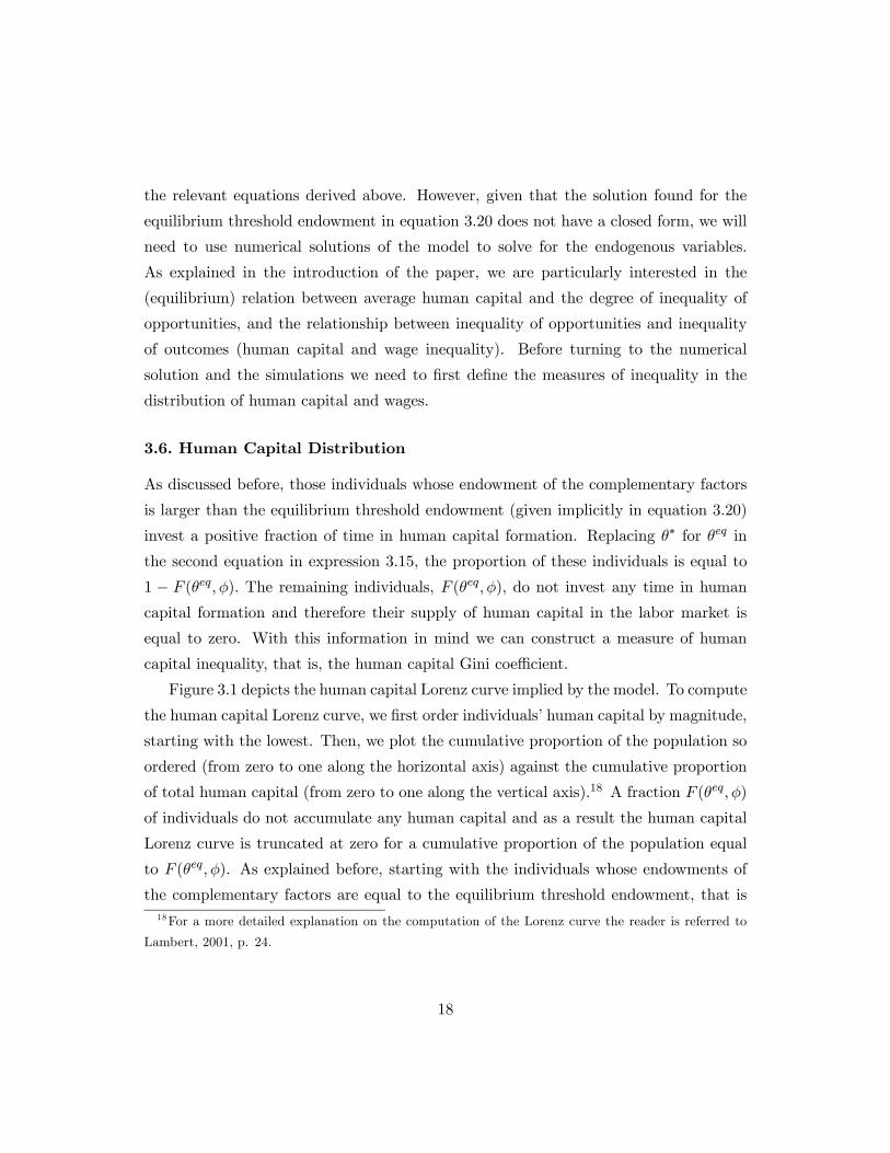
3.6. Human Capital Distribution
As discussed before, those individuals whose endowment of the complementary factors
is larger than the equilibrium threshold endowment (given implicitly in equation 3.20)
invest a positive fraction of time in human capital formation. Replacing θ∗ for θeq in
the second equation in expression 3.15, the proportion of these individuals is equal to
1 − F (θeq,φ). The remaining individuals, F (θeq,φ), do not invest any time in humancapital formation and therefore their supply of human capital in the labor market is
equal to zero. With this information in mind we can construct a measure of human
capital inequality, that is, the human capital Gini coefficient.
Figure 3.1 depicts the human capital Lorenz curve implied by the model. To compute
the human capital Lorenz curve, we first order individuals’ human capital by magnitude,
starting with the lowest. Then, we plot the cumulative proportion of the population so
ordered (from zero to one along the horizontal axis) against the cumulative proportion
of total human capital (from zero to one along the vertical axis).18 A fraction F (θeq,φ)
of individuals do not accumulate any human capital and as a result the human capital
Lorenz curve is truncated at zero for a cumulative proportion of the population equal
to F (θeq,φ). As explained before, starting with the individuals whose endowments of
the complementary factors are equal to the equilibrium threshold endowment, that is18For a more detailed explanation on the computation of the Lorenz curve the reader is referred to
Lambert, 2001, p. 24.
18

the individuals with θi = θeq, individuals supply positive amounts of human capital in
the labor market. As a result, in Figure 3.1, after the individual with θi = θeq, the
cumulative proportion of total human capital is greater than zero and increasing in θi,
and therefore increasing as we move to the right of the graph.19
% of totalhuman capital
1
A
B
0 1 % of individuals
045
( , )eqF θ φ 1 ( , )eqF θ φ−
Figure 3.1: Human Capital Lorenz Curve
Using Figure 3.1, the human capital Gini coefficient is defined as:20
Ginih =A
A+B(3.21)
The larger the human capital Gini coefficient is, the more unequal is the distribution of19Figure 5.1 in Appendix (B) presents the Education Lorenz curves for two countries (Korea and
India) in two points in time (1960 and 1990) for each country. Note that the pattern of the Lorenz
curves predicted in the model (the fact that they are truncated) is observed in the actual data. The
reader is referred to Thomas et al. (2002) for details.20The Gini coefficient is an area measure of how far the Lorenz curve is from the 45 degree line (the
perfect equality line). The further away the Lorenz curve is from the 45 degree line, the higher is the
degree of inequality in the distribution of human capital in the population.
19

human capital across individuals.
Using the equation that relates each individual’s supply of human capital in the
labor market to her endowments of the complementary factors (equation 3.9), and the
distribution of these endowments across the population, we can derive the distribution of
human capital across individuals using the change of variable technique. However, note
that those individuals in the population with a lower endowment than the equilibrium
threshold endowment do not accumulate any human capital. Formally, human capital
is distributed across individuals according to the following probability distribution:
Pr(h = 0) = F (θeq,φ)
Pr(h < h) = F (θeq,φ) +
Z h
h(θeq)g(h,φ)dh for h ∈ [h(θeq), h(
_θ)]
, (3.22)
where: g(h,φ) = f [θ(h),φ]
¯dθ
dh
¯; h(θeq) is the human capital supplied in the labor
market by the individual with an endowment of the complementary factors equal to
the equilibrium threshold endowment, that is, the individual with θi = θeq; h(_θ) is
the human capital supplied in the labor market by the individual with the highest
endowment of the complementary factors in the population, that is, the individual with
θi =_θ; 21 f(.) is the density function associated with the CDF F (.); θ(h) and
dθ
dhcan
be obtained from equation 3.9.
Having found the distribution of human capital across individuals, the human capital
Gini coefficient is defined by:22
Ginih = 2
Z h(_θ)
h(θeq)hG(h,φ)g(h,φ)dh− 1, (3.23)
where: G(h,φ) =Z h
h(θeq)g(h,φ)dh.
Equation 3.23 will be used in the next section when we solve the model numerically
and examine how inequality in the distribution of opportunities affects inequality in the21h(θeq) and h(θ) are obtained by evaluating equation 3.9 at θi = θeq and θi = θ respectively.22See Lambert (2001), chapter 2.
20

distribution of human capital. In other words, how inequality of opportunities affects
inequality of outcomes.
3.7. Wage Income Distribution
We have assumed that agents differ only regarding their endowment of the comple-
mentary factors to the educational process. Although this is a strong assumption it is
valid if we want to concentrate on the effects of inequality of opportunities on human
capital accumulation and inequality of outcomes. A more complete model would have
to assume also heterogeneity of wealth, and one can plausibly expect the two sources of
heterogeneity across individuals to be highly correlated. For the moment we will assume
that all agents are endowed with the same share of the aggregate capital stock and we
will concentrate on the distribution of wage income.
Replacing θ∗ by the equilibrium threshold endowment, θeq, in equations 3.13 and
3.14, and using the distribution of human capital across individuals (equation 3.22), we
can construct the wage income Lorenz curve (see Figure 3.2).23
From Figure 3.2, a fraction F (θeq,φ) of individuals work as unskilled labor and
all receive the same wage income, given by the unskilled wage rate, wu. Individuals
with an endowment of the complementary factors larger than the equilibrium threshold
endowment receive wage income equal to wsγγ
(1 + γ)1+γ(1 + θi)
γ .
Using the information in Figure 3.2, the wage income Gini coefficient is given by:
Giniw =A
A+B(3.24)
The definition of wage inequality in expression 3.24 will be used in the next section
to solve for the degree of inequality in the distribution of wage income.
3.8. Inequality of Opportunities and Average Human Capital
This section examines the relation between inequality of opportunities and average
human capital in the economy.23The computation of the wage income Lorenz curve follows the same steps as the computation of
the human capital Lorenz curve described above.
21

% of totaltotal wage income
1
A
B
0 1% of individuals
045
( , )eqF θ φ 1 ( , )eqFθ φ−
Figure 3.2: Wage Income Lorenz Curve
Recall that the distribution of the complementary factors to the educational process
is determined by the cumulative distribution function F (θ,φ) , where the parameter φ
measures the degree of equality in the distribution of endowments (the degree of equality
of opportunity).
After replacing for the equilibrium threshold endowment (θeq) in equation 3.16, the
marginal change in average human capital that results from a marginal change in the
degree of equality of opportunity is given by:
dh
dφ= Λ
⎡⎣Z _θ(φ)
θeq(φ)(1 + θ)γ
∂f(θ,φ)
∂φdθ − (1 + θeq)γf (θeq,φ)
dθeq
dφ+ (1 +
_θ)γf(
_θ,φ)
d_θ
dφ
⎤⎦ ,(3.25)
where Λ =γγ
(1 + γ)1+γ, and
dθeq
dφcan be obtained from equation 3.20 using the implicit
function theorem.
The first term of the bracketed expression on the right hand side of equation 3.25
captures the marginal change in human capital (across the skilled individuals) that
22

results from the marginal change in the density of the distribution of endowments caused,
in turn, by a marginal change in the degree of equality. The second term captures the
marginal change in human capital that results from a marginal change in the equilibrium
threshold endowment (i.e., how much human capital is accumulated by the individuals
with θi = θeq, times the corresponding marginal change in θeq). The third term captures
the marginal change in human capital that results from a marginal extension/contraction
of the upper bound of the support of the distribution of endowments that results from
a marginal change in the degree of equality. The last term measures how much human
capital is accumulated by those individuals with the highest endowment, times the
corresponding change in this endowment level that results from a marginal change in
degree of equality in the distribution of endowments.
In the following section we will use a specific distribution function for the endow-
ments of the complementary factors that allows for changes in the degree of equality in
the distribution while keeping the mean endowment in the population constant. This
exercise will allow us to understand how average human capital changes as the degree
of equality in the distribution of endowments increases, while keeping the mean endow-
ment in the population constant. Also, the numerical simulations will tell us how each
of the components in equation 3.25 affects the average level of human capital as the
degree of equality of opportunity increases.
4. Numerical simulations
This section presents the numerical solution of the model as well as the main results of
the simulation of two different kind of interventions on the distribution of endowments.
We begin by specifying a (well behaved) distribution function for the endowments of
the complementary factors to the schooling process and then implement two kind of
interventions. First, we simulate a change in the degree of equality in the distribution
of endowments keeping the mean endowment in the population constant (a mean pre-
serving spread in the distribution of endowments), and second, we simulate a change in
23
the support of the distribution keeping the other parameters of the model constant.24
Once the two different interventions are simulated, we will be able to explain how human
capital and its distribution across individuals changes as the degree of equality in the
distribution of endowments of the complementary factors changes. In other words, using
the equations derived in the previous section, the numerical simulations will allow us
to disentangle the equilibrium relationships between inequality of opportunities (that
is, inequality of endowments of the complementary factors to the schooling process),
inequality of outcomes (inequality in the distribution of human capital and of wage in-
come), and the degree of efficiency in human capital formation (as measured by average
human capital in the economy).
Recall that the cumulative distribution function of endowments of the complemen-
tary factors to the schooling process across the population is denoted by F (θ,φ). Let
F (θ,φ) take the following functional form:
F (θ,φ) =
⎧⎪⎪⎪⎪⎪⎨⎪⎪⎪⎪⎪⎩0 for θ < 0∙
φ
1 + φ
¸φθφ for θ ∈
h0, 1+φφ
i1 for θ >
1 + φ
φ
, (4.1)
with φ ∈ [ γ1−γ , 1].
25
Some of the characteristics of the cumulative distribution function, F (θ,φ), described
in equation 4.1 are:
(i) Mean: E(θ) = 1 ∀φ(ii) Median: F (θm) =
1
2⇒ θm =
1 + φ
φ21/φ
(iii) As φ → 1, the distribution function in equation 4.1 approaches the Uniform
distribution.24Altough the two interventions impose strong restrictions in the kind of changes in the distribution
that we permit, they allow us to isolate changes in the dispersion of the distribution from changes in
the mean, and viceversa.25Recall that we had the following restriction:
_
θ < 1γ(see footnote # 14). We will assume that the
upper bound of the domain satisfies: 1+φφ< 1
γ, which is equivalent to : γ
1−γ ≤ φ.
24

(iv) Define the first measure of inequality in the distribution of θ as: Ω =median
mean.
That is:
Ω =1 + φ
φ21φ
where: Ω ∈ [ 1
γ21−γγ
, 1]. (4.2)
A higher value of Ω corresponds to a higher degree of equality (because the median
of the distribution is closer to the mean). Note also that:
∂Ω
∂φ> 0 for φ ∈ [ γ
1− γ, 1]
Therefore, both φ and Ω are measures of equality in the distribution of endowments
of the complementary factors.
(v) Define the Gini coefficient of the distribution θ as:26
Giniθ = 2
Z 1+φφ
0θF (θ,φ)f(θ,φ)dθ − 1 (4.3)
Solving the previous equation using the distribution given in equation 4.1 we have:
Giniθ =2(1 + φ)
2φ+ 1− 1
Using the last equation, note that:∂Giniθ∂φ
< 0. Not surprisingly, as the parameter
that captures the degree of equality in the distribution of endowments increases, the
Gini coefficient, which is a measure of inequality in the distribution of endowments,
decreases.
4.1. First Intervention: A Change in Inequality of Opportunities
Given that the mean of the distribution specified in equation 4.1 is constant for all
values of the parameter φ, any change in this last parameter modifies the shape (disper-
sion) of the distribution while leaving the mean unchanged. We will make use of this
characteristic of the distribution to carry out the first simulation.26See Lambert (2001), chapter 2.
25
This exercise will allow us to concentrate on the changes in the endogenous variables
of the model that arise from changes in the degree of inequality of the distribution of
endowments while maintaining fixed the mean endowment .
To carry out the simulation we begin by fixing some parameters of the model,27 and
solve for the equilibrium values of the endogenous variables for different values of φ, for
φ ∈ [ γ1−γ , 1].
The first (and main) step to solve the model numerically is to find the value of θeq
that solves equation 3.20 using the distribution function in equation 4.1 for different
values of the parameter φ. Once we have the numerical solution for the equilibrium
threshold endowment, θeq, for each value of φ in the interval [ γ1−γ , 1], we replace it in
the relevant equations derived in the previous section, along with the other parameter
values used, to obtain the corresponding values of the endogenous variables of the model.
The results of the simulation of the first intervention are presented in the panels of
Figure 4.1.28 From Panel (A), as equality of opportunity in the distribution of endow-
ments, as captured by the parameter Ω (see equation 4.2), increases, average human
capital in the population also increases. Conversely, a more unequal distribution of op-
portunities is associated with a lower level of average human capital across individuals.
Panel (B) depicts the relationship between average human capital and a measure of in-
equality in the distribution of human capital across individuals, the human capital Gini
coefficient. A lower level of average human capital is associated with a more unequal
distribution of human capital (a higher human capital Gini). Panel (C) graphs the27We use the following parameter values for the simulation: α = 0.3, β = 0.3, K = 10 and γ = 0.15.
The first two parameters measure the elasticities of output with respect to unskilled labor and human
capital respectively. The values chosen for these two parameters are close enough to those found in
the empirical growth literature (see Mankiw, Romer and Weil, 1992). The qualitative results of the
simulation do not change with the size of the capital stock chosen, K = 10. Regarding the parameter γ,
which measures the elasticity of human capital with respect to time investment, we chose a value such
that the technology of human capital formation was sufficiently concave. However, the results of the
simulation are maintained for different values of this parameter that satisfy the restriction imposed on
this parameter in footnote # 25.28The different curves presented in Figure 4.1 are not ‘smooth’ because the simulation of the model
involves numerical approximations of integrals and of the solutions to non-linear equations.
26

relationship between inequality of opportunities and inequality of outcomes in human
capital formation. The higher the degree of inequality of opportunities is, the higher
the degree of inequality in the distribution of human capital across individuals. In other
words, a higher inequality of opportunities leads to a higher inequality of outcomes (in
terms of the accumulation of human capital). Panel (D) shows the relationship between
inequality of opportunities, as measured by the Gini coefficient of the distribution of
endowments, and wage inequality. A higher degree of inequality of opportunities is
associated with a more unequal distribution of wage income. Panel (E) shows that the
higher the inequality of opportunities is, the larger is the fraction of individuals who de-
cide not to acquire human capital and work as unskilled workers. Also, a more unequal
distribution of human capital across individuals is associated with a higher fraction of
the population not investing time in human capital formation and working as unskilled
workers (panel F).
Summarizing the results obtained so far, a higher degree of inequality of opportuni-
ties is associated with lower average human capital, higher inequality in the distribution
of human capital, higher wage inequality and a lower fraction of individuals in the pop-
ulation investing in human capital formation.
The main finding of this section is the lack of an efficiency-equity trade-off in human
capital formation. In other words, the relation between average human capital and the
degree of inequality in the distribution of human capital obtained from the simulation
of the model is negative.29 Also, according to the numerical simulations, there is a
direct relationship between equality of opportunities and equality of outcomes, not only
in terms of human capital but also in terms of wage income.
From the simulation of the model we can also disentangle the different forces behind
the main result of this section, namely, the different forces behind the positive relation
between equality of opportunity and the average level of human capital in the economy.
Recall that the change in human capital that results from a change in the degree of
equality of opportunity can be decomposed into three different factors (see equation
3.25 and the explanation thereafter). From equation 4.1, we know that the last term in29This finding matches the main stylized fact regarding the relation between these two variables
described in the introductory section of the paper (see Figure 2.1).
27

( D ) ( E )C F
B E
A D
Figure 4.1: Simulation Results: Mean Preserving Spread
28

the bracketed expression in equation 3.25 is negative, that is:d_θ
dφ= − 1
φ2< 0. Also, we
know from the results of the simulation that the second term is positive, since we find
that:dθeq
dφ> 0. Therefore, given that we have found that human capital (h) increases
with equality of opportunity (φ), the first term in the right hand side of equation
3.25 is positive. In words, this means that the increase in average human capital in
the economy results from two counteracting forces. On the one hand, average human
capital increases with equality of opportunities as the human capital among the skilled
individuals increases. On the other hand, average human capital decreases because,
first, the equilibrium threshold endowment increases with equality and therefore the
economy “loses” the human capital accumulated by those individuals with θi = θeq
times the size of the increase in θeq. And second, the upper bound of the support
decreases, so the economy also “loses” the human capital of those individuals with the
highest endowments, that is the human capital of those individuals with θi =_θ, times
the size of the decrease in_θ that results form the change in the degree of equality of
opportunity. We also know from the results of the simulation that the change in the
density of individuals that results from a change in equality of opportunity is sufficiently
large to offset the two negative effects just described.
The intuition behind the positive relation found between equality of opportunity and
the average level of human capital is the following: first, a higher degree of equality in
the distribution of opportunities implicitly implies a reallocation of the complementary
factors to the schooling process from individuals with a high endowment towards indi-
viduals with a low endowment,30 keeping the mean endowment fixed. Second, under
the assumption that the returns to time investment in human capital formation are de-
creasing, individual’s human capital supplied in the labor market is a concave function
of her endowment of the complementary factors (equation 3.9). And third, note that
the general equilibrium model takes into account the endogenous labor supply response
that results from a higher degree of equality of opportunity in human capital forma-30Our model, however, doesn’t specify the mechanism by which this redistribution takes place. The
models by Benabou (2000) and Galor and Moav (2003) explicitly specify this mechanism.
29

tion.31 The results from the simulations of the model, which combine the three elements
described above, show that a higher degree of equality of opportunity is associated with
a higher average level of human capital in the economy. Conversely, the human capital
“forgone” by decreasing the endowments of those individuals who are relatively better
off is more than offset by the additional human capital that is acquired by those indi-
viduals who, after the implicit redistribution of resources, choose to invest a positive
fraction of their time in human capital formation.
4.2. Second Intervention: A Change in the Support of the Distribution of
Opportunities
In the second exercise we fix the parameter φ and shift the whole distribution of en-
dowments. That is, we change the support of the distribution F (θ,φ) while keeping the
parameter φ fixed. The cumulative distribution function is now given by:
F (θ,φ) =
⎧⎪⎪⎪⎪⎪⎨⎪⎪⎪⎪⎪⎩0 for θ < 0∙
φ
1 + φ
¸φ(θ − z)φ for θ ∈
hz, z + 1+φ
φ
i1 for θ >
1 + φ
φ
, (4.4)
where we allow the parameter z to vary between [0, 1].
We assume throughout this section the same parameter values that we used in the
first exercise and, as a benchmark, we fix φ = 0.5.
When we change the parameter z, it is as if each individual in the economy were
given an additional fixed quantity of the complementary factors to the schooling process.
The mean endowment in this case changes linearly with z.32 In this exercise, changes in
average human capital across all individuals are expected to be positive as z increases,
because each agent has a higher endowment of the complementary factors to the school-
ing process. However, we are interested in the relationship between average human31That is, the change in the equilibrium threshold endowment that results from a change in the degree
of equality.32The mean endowment in this case is given by: E(θ) = 1 + z
30

capital, inequality of opportunities, inequality in the distribution of human capital and
wage inequality.
The reader can easily derive the characteristics of the new distribution function that
correspond to points (i) through (v) in the last subsection.
The simulation in this case is very similar to the one carried out in the first exercise,
except that we now fix the parameter φ and allow the parameter z to change in the
interval [0, 1].
As in the previous simulation, the first step to solve the model numerically is to
find the value θeq that solves equation 3.20 using the distribution function described
in equation 4.4, for each value of the parameter z in the interval [0, 1]. Once we have
the solution for θeq for the different values of z we can use the equations derived in the
previous section to obtain the corresponding values of the endogenous variables of the
model.
The results of the second simulation are presented in the panels of Figure 4.2. From
Panel (A), a higher degree of equality of opportunity, as captured by the ratio median
over mean, is associated with a higher level of average human capital. This results is
confirmed by Panel (B), where the relationship between human capital inequality (as
measured by the human capital Gini) and average human capital is negative. Panels
(C) and (D) say that more inequality of opportunities is associated with more inequality
in the distribution of human capital and more wage inequality. Panel (E) says that the
higher the inequality of opportunities is, the higher is the number of individuals that do
not invest time in human capital formation and work as unskilled labor. Finally, Panel
(F) says that higher inequality in the distribution of human capital is associated with
a larger number of unskilled individuals in the population.
Summarizing, the results in this section match the results obtained in the first simu-
lation. Namely, they confirm the positive relationship between equality of opportunities
and average human capital in the economy, and the positive relation between equality
of opportunities and equality of outcomes, also found in the simulation of the first in-
tervention. However, the two interventions are different in nature. While the first one
changes the degree of inequality keeping the mean endowment constant, the second one
31

C F
B E
A D
Figure 4.2: Simulation Results: Change in the Support of the Distribution32

shifts the whole distribution of endowments to the right while leaving the shape of the
cumulative distribution function unchanged.
5. Concluding Remarks
This paper develops a heterogeneous agent general equilibrium model with unequal op-
portunities in human capital formation. The model presented explains, among other
things, the negative relation between average human capital and human capital inequal-
ity. While most of the existing literature suggests an explanation for the negative rela-
tion between these two variables based on the existence of credit market imperfections
(that prevent poor individuals from investing in human capital), our model explores a
different, and, perhaps complementary explanation. Namely, our explanation is based
on the existence of different rates of return to time invested in the accumulation of
human capital across individuals, which are, in turn, determined by each individual’s
endowment of the complementary factors to the schooling process. In other words, the
model specifies inequality of opportunities in human capital formation across individuals
as a differential endowment of the factors that complement the schooling process.
In equilibrium, the endogenous variables of the model are determined, among other
parameters, by the degree of inequality in the distribution of the endowments that com-
plement the schooling process. In order to study the relation between the endogenous
variables of the model and the parameters, we solve the model numerically using a dis-
tribution function for the endowments of the complementary factors that allows us to
isolate changes in the degree of equality from changes in the mean endowment. Using
numerical simulations we examine how the endogenous variables of the model respond
to two different interventions in the distribution of opportunities: a mean-preserving
spread, and a change in the support of the distribution. Among the main results, we
find that a higher degree of inequality of opportunities is associated with a lower aver-
age human capital in the population, a lower fraction of individuals investing in human
capital, a higher degree of inequality in the distribution of human capital, and a higher
degree of wage inequality.
33

References
Aghion P., E. Caroli and C. Garcia-Peñalosa, 1999, “Inequality and Economic
Growth: The Perspective of the New Growth Theories”, Journal of Economic Literature,
vol. XXXVII, December.
Angrist, J., E. Bettinger, ,E. Bloom, ,E. Kling, , and M. Kremer, 2003,
“Vouchers for Private Schooling in Colombia: Evidence from a Randomized Natural
Experiment”, American Economic Review, 92(5), December.
Banerjee, A.V. and A.F. Newman, 1993, “Occupational Choice and the Process
of Development”, Journal of Political Economy, 101(2): 274-298.
Barro, R.J., 2001, “Human Capital and Growth”, American Economic Review,
May, 91(2), 12-17.
Bénabou, R., 1996, “Equity and Efficiency in Human Capital Investment: The
Local Connection”, Review of Economic Studies, 62, 237-264.
Bénabou, R., 2000, “Meritocracy, Redistribution, and the Size of the Pie”, in
Arrow et al. Meritocracy and Economic Inequality, Princeton University Press.
Bénabou, R., 2000, “Unequal Societies: Income Distribution and the Social Con-
tract”, American Economic Review, 90, 96-129.
Benhabib, J. and M.M. Spiegel, 1994, “The Role of Human Capital in Eco-
nomic Development: Evidence From Aggregate Cross-Country Data”, Journal of Mon-
etary Economics, 34, 143-173.
Benhabib, J. and M.M. Spiegel, 2003, “Human Capital and Technology Diffu-
sion”, forthcoming in Aghion and Durlauf eds., Handbook of Economic Growth, North
Holland, Amsterdam.
Betts, J. and D. Morell, 1999, “The Determinants of Undergraduates Grade
Point Average: The relative Importance of Family Background, High School Resources,
and Peer group Effects”, Journal of Human Resources, 34, 2, 268-293.
Bobonis, G., E. Miguel, and C. Sharma, 2002, “Iron Supplementation and
Early Childhood Development: A Randomized Evaluation in India.” Mimeo, U.C.
Berkeley.
34

Bourguignon, F., F. Ferreira and M. Menéndez, 2003, “Inequality of Out-
comes and Inequality of Opportunities in Brazil”, Working Paper # 3174, World Bank.
Carneiro, P., and J. Heckman, 2002, “Human Capital Policy”, in Heckman and
Krueger, Inequality in America, MIT Press.
Dardanoni, V., G. Fields, P. Roemer and M. Sanchez, 2003, “How demand-
ing should equality of opportunity be, and how much have we achieved”, unpublished
manuscript.
De Gregorio, J., 1996, “Borrowing constraints, human capital accumulation, and
growth”, Journal of Monetary Economics 37, 49-71.
Duflo, E. and M. Kremer, 2003, “Use of Randomization in the Evaluation of
Development Effectiveness”, mimeo, MIT.
Durlauf, S., 1996, “Neighborhood Feedbacks, Endogenous Stratification, and In-
come Inequality”, in: Barnett, Gandolfo, and Hillinger eds., Dynamic Disequilibrium
Modelling, Cambridge, Cambridge university Press.
Durlauf, S., 2002, “Groups, Social Influences and Inequality: A Membership The-
ory Perspective on Poverty Traps”, University of Wisconsin..
Fernandez, R. and Rogerson, 1996, “Keeping People Out: Income Distribution,
Zoning, and the Quality of Public Education”, Quarterly Journal of Economics, 38, 1,
25-42.
Flug, K, A. Spilimbergo and E. Wachteinheim, 1998, ”Investment in edu-
cation: do economic volatility and credit constraints matter?” Journal of Development
Economics 55, 465-481.
Galor, O. and J. Zeira, 1993, “Income Distribution and Macroeconomics”, Re-
view of Economic Studies, 60: 35-52.
Galor, O. and D. Tsiddon, 1997, “Technological Progress, Mobility, and Eco-
nomic Growth”, American Economic Review, Vol. 87, No. 3, 363-382.
Galor, O., and O. Moav, 2003, “Das Human Kapital”, mimeo, Brown University.
Ginther, D., R. Haveman and B. Wolfe, 2000, “Neighborhood Attributes as
Determinants of Children’s Outcomes: How Robust are the Relationships”, Journal of
Human Resources, Vol. 35, No. 4, 603-642.
Goldhaber, D. and D. Brewer, 1997, “Why don’t Schools and Teachers Seem to
35

Matter? assessing the Impacts of Unobservables on Educational Productivity”, Journal
of Human Resources, 32, 3, 505-523.
Grogger, G., 1997, “Local Violence and Educational Attainment”, Journal of
Human Resources, 32, 4, 659-682.
Handa, S., 2002, “Raising Primary School Enrolment in Developing Countries,
The Relative Importance of Supply and Demand”, Journal of Development Economics,
69, 103-128.
Hanushek, E., 1986, “The Economics of Schooling: Production and Efficiency in
Public Schools”, Journal of Economic Literature, vol. 24, No. 3, 1141-1177.
Hanushek, E., 1996, “Measuring Investment in Education”, Journal of Economic
Perspectives, Vol. 10, No. 4, 9-30.
Kremer, M., 2003, “Randomized Evaluation of Educational Programs in devel-
oping Countries: Some Lessons, forthcoming in American Economic Review P&P.
Lambert, P., 2001, The Distribution and Redistribution of Income, Manchester
University Press.
Lucas, R., 1988, “On the Mechanics of Economic Development”, Journal of Mon-
etary Economics, 22, 3-42.
Mankiw, N.G., D. Romer, and D.N. Weil, 1992. “A Contribution to the
Empirics of Economic Growth”, Quarterly Journal of Economics, 407-437.
Mejía, D., 2003, “Inequality, Credit Market Imperfections and Human Capital
Accumulation”, paper presented at the 8th Annual Meeting of LACEA, Puebla, Mexico.
Roemer, J., 2000, “Equality of Opportunity”, in Arrow et al. Meritocracy and
Economic Inequality, Princeton University Press.
Schultz, T.P., 1988, “Education Investment and Returns”, in Chenery and Srini-
vasan, eds., Handbook of Development Economics, Amsterdam, North Holland.
Schultz, T.P., “School Subsidies for the Poor: Evaluating the Mexican Progresa
Poverty Program”, Journal of Development Economics, forthcoming.
Thomas, V., Y. Wang and X. Fan, 2002, “A New Dataset on Inequality in
Education: Gini and Theil Indices of Schooling for 140 Countries, 1960-2000”, World
Bank.
36
Appendix
(A1)
Note that from equation 3.8, b(u∗i ) =µ
γ
1 + γ(1 + θi)
¶γ
denotes the optimal level
of human capital for individual i. Recall that θi is different for all individuals and is
determined by each agent’s endowment of the complementary factors to the educational
process . Let, only as an example, the endowment be a weighted average33 of two
characteristics: parental level of education (εi) and an a measure of health (κi) . Thatis, let: 1 + θi = δελi κ
1−λi , with δ and λ being unknown parameters to the researcher. If
parental level of education and health characteristics are observed for each individual
and we are able to proxy b(u∗i ) with test scores, or by an indicator of years of schooling for
each individual (si) then, the effects of parental education and health can be estimated
from the log-linearization of the optimal amount of human capital derived above. That
is:
ln si = const+ γλ ln εi + γ(1− λ) lnκi. (A1)
From the estimation of the above equation, a researcher can estimate the effects of
different characteristics of the individual on observed educational outcomes. In many
of the empirical studies reviewed in the introduction, this is the form that is estimated.33 It is not necessary that the weights add up to 1, but is a hypothesis that can be tested.
37

(A2)
Proof of Proposition 1
There exists a unique equilibrium solution under a fairly general context. The market
solution exists if there is an equilibrium threshold endowment, θeq, which is a root of the
following non linear function in θ for any given parameters γ,α,β ∈ (0, 1), and φ ∈ E.p(θ,α,β, γ,φ) = k(θ,α,β, γ,φ)− g(θ, γ,φ),where k(θ,α,β, γ,φ) = β
α(1 + θ)γFφ(θ), g(θ, γ,φ) =R θθ (1 + y)
γfφ(y)dy, fφ(.) is a
probability density function of the endowments and D = [θ, θ] is the support of the
distribution fφ(.).
(Existence) First, note that k(.) is strictly increasing in θ and that g(.) is non-
increasing in θ. Thus, p(.) is strictly increasing in θ. If fφ(.) is Riemann integrable,
p(.) is continuous, and the image of D is a compact and a connected subset of the real
numbers. That is, the image is a bounded and closed interval, which we will denote by
I = [a, b] ⊂ R. Since p(.) is strictly increasing, a = p(θ,α,β, γ,φ) = k(θ,α,β, γ,φ) −g(θ, γ,φ) = − R θθ (1+y)γfφ(y)dy < 0 and b = p(θ,α,β, γ,φ) = β
α(1+θ)γ > 0. Therefore,
0 ∈ I so that there exists θeq ∈ (θ, θ) for which p(θeq,α,β, γ,φ) = 0.(Uniqueness) Since p(.) is strictly increasing on D, it is injective and, therefore, a
unique equilibrium solution exists. Q.E.D.
Remark: The only assumption we impose on fφ(.) is Riemann integrability. Con-
tinuous or piecewise continuous functions are particular cases of Riemann integrable
functions.
Sketch of the proof of Proposition 2
Let Leq = F (θeq,φ) be the fraction of the population working as unskilled labor in
equilibrium. Note that equation 3.20 can be rewritten as: MPLu(Leq)
MPH(Leq) =γγ
(1+γ)1+γ(1 +
θeq)γ . This last equation is equivalent to the following expression: MPLu(Leq) =
MPLs(Leq) =MPH(Leq)dH(Leq)
dLs , by noticing that dH(Leq)
dLs = γγ
(1+γ)1+γ (1 + θeq)γ, which
we show next.
38

Assume that fφ is strictly positive ∀φ ∈ E, so that given any measure of unskilledworkers Lu, there is a (unique) corresponding threshold θ(Lu). That is, using the
implicit function theorem in equation Lu = F (θ,φ), there exists a function θ : (0, 1)→ D
that associates to each Lu a θ(Lu), such that Lu = F (θ(Lu),φ). With this in mind, the
total human capital function is defined by H(Lu) = γγ
(1+γ)1+γ
R θθ(Lu)(1+θ)
γf(θ,φ)dθ with
0 ≤ Lu ≤ 1. This function defines the level of human capital in the economy given thata fraction Lu of the population works as unskilled labor. Assuming differentiability we
have that: dH(Lu)dLu = − γγ
(1+γ)1+γ(1 + θ(Lu))γf(θ(Lu),φ)dθ(L
u)dLu < 0. The last expression
can be simplified by noticing that dθ(Lu)
dLu = 1f(θ(Lu),φ) . Hence,
dH(Lu)dLu = − γγ
(1+γ)1+γ(1 +
θ(Lu))γ . That is, the marginal reduction in total human capital that results from a
marginal increment in the measure of unskilled workers is exactly equal to the human
capital contribution of the marginal individual with endowment θ(Lu). Hence, dH(Leq)
dLs =γγ
(1+γ)1+γ (1 + θeq)γ since dH(Lu)dLu = −dH(Lu)dLs .
Thus, in equilibrium, the allocation of individuals between skilled and unskilled
occupations is done in such a way that the marginal productivity of the individual with
an endowment θi = θeq is the same for both occupations. This is indeed a necessary
and sufficient condition for maximizing total output.34
34The reader can check that the equation MPLu(Leq) =MPLs(Leq) is both, a sufficient and neces-
sary first order condition for the following output maximization problem:
MaxLu,Ls
F (Lu,H,K)
s.t.:
Lu + Ls = 1, H = γγ
(1+γ)1+γ
R θθ(Lu)
(1 + θ)γf(θ(Lu),φ)dθ, and Lu = F (θ(Lu),φ)
39

(B)
Source: Thomas et al. (2000)
Education Lorenz Curve, India 1960
0.0
75.7
0.0
100.0
96.6100.0
0.0
37.2
95.5
0
20
40
60
80
100
0 20 40 60 80 100Cumulative Proportion of Population Distribution
(%)
Cum
ulat
ive
Prop
ortio
n of
Sch
oolin
g (%
)
Q
PO
S
Mean=1.09 yearsEducation Gini = .79
Education Lorenz Curve, Korea 1960
0.0
48.2
0.0
68.7
2.70.0
94.490.3
100.0
0
20
40
60
80
100
0 20 40 60 80 100Cumulative Proportion of Population Distribution
(%)
Cum
ulat
ive
Prop
ortio
n of
Sch
oolin
g(%
)
Q
PO
S
Mean=4.27 yearsEducation Gini = .55
Education Lorenz Curve, India 1990
0.0
23.8
0.0
100.0
83.8
91.0
0.010.9
63.3
0
20
40
60
80
100
0 20 40 60 80 100Cumulative Proportion of Population Distribution
(%)
Cum
ulat
ive
Prop
ortio
n of
Sch
oolin
g (%
)
Q
PO
S
Mean=2.95 yearsEducation Gini = .69
Education Lorenz Curve, Korea 1990
0.09.4
24.9
0.20.0
89.2
78.3
100.0
0
20
40
60
80
100
0 20 40 60 80 100Cumulative Proportion of Population Distribution
(%)
Cum
ulat
ive
Prop
ortio
n of
Sch
oolin
g (%
)
Q
PO
S
Mean=10.04 yearsEducation Gini = .22
Figure 5.1: Education Lorenz Curves: India and Korea, 1960 and 1990
40