Embed Size (px)
Citation preview
Underwater Wireless Video Transmission using Acoustic OFDM
Jordi Ribas, Massachusetts Institute of TechnologyE-mail: [email protected]
Advisor: Milica Stojanovic, Northeastern UniversityE-mail: [email protected]
December 27, 2009


Contents
1 Introduction 191.1 Background . . . . . . . . . . . . . . . . . . . . . . . . . . . . . . . . . . . . . . . . . . . . . . 191.2 Approach . . . . . . . . . . . . . . . . . . . . . . . . . . . . . . . . . . . . . . . . . . . . . . . 201.3 Objectives . . . . . . . . . . . . . . . . . . . . . . . . . . . . . . . . . . . . . . . . . . . . . . . 201.4 Project workplan . . . . . . . . . . . . . . . . . . . . . . . . . . . . . . . . . . . . . . . . . . . 21
2 The underwater channel 232.1 Acoustic propagation . . . . . . . . . . . . . . . . . . . . . . . . . . . . . . . . . . . . . . . . . 23
2.1.1 Attenuation . . . . . . . . . . . . . . . . . . . . . . . . . . . . . . . . . . . . . . . . . . 232.1.2 Noise . . . . . . . . . . . . . . . . . . . . . . . . . . . . . . . . . . . . . . . . . . . . . 242.1.3 Propagation delay . . . . . . . . . . . . . . . . . . . . . . . . . . . . . . . . . . . . . . 262.1.4 Multipath . . . . . . . . . . . . . . . . . . . . . . . . . . . . . . . . . . . . . . . . . . . 262.1.5 Doppler effect . . . . . . . . . . . . . . . . . . . . . . . . . . . . . . . . . . . . . . . . . 27
2.2 Resource allocation . . . . . . . . . . . . . . . . . . . . . . . . . . . . . . . . . . . . . . . . . . 272.2.1 The AN product and the SNR . . . . . . . . . . . . . . . . . . . . . . . . . . . . . . . 272.2.2 Optimal frequency . . . . . . . . . . . . . . . . . . . . . . . . . . . . . . . . . . . . . . 272.2.3 3 dB bandwidth definition . . . . . . . . . . . . . . . . . . . . . . . . . . . . . . . . . . 282.2.4 Transmission power . . . . . . . . . . . . . . . . . . . . . . . . . . . . . . . . . . . . . 28
3 Video compression techniques 313.1 Compression fundamentals . . . . . . . . . . . . . . . . . . . . . . . . . . . . . . . . . . . . . . 31
3.1.1 Images and video . . . . . . . . . . . . . . . . . . . . . . . . . . . . . . . . . . . . . . . 313.1.2 Compression approaches . . . . . . . . . . . . . . . . . . . . . . . . . . . . . . . . . . . 33
3.2 MPEG-4 standard . . . . . . . . . . . . . . . . . . . . . . . . . . . . . . . . . . . . . . . . . . 353.2.1 Functionalities . . . . . . . . . . . . . . . . . . . . . . . . . . . . . . . . . . . . . . . . 353.2.2 Very Low Bit-rate Video core . . . . . . . . . . . . . . . . . . . . . . . . . . . . . . . . 35
3.3 Implementation . . . . . . . . . . . . . . . . . . . . . . . . . . . . . . . . . . . . . . . . . . . . 363.3.1 MPEG-4 codec . . . . . . . . . . . . . . . . . . . . . . . . . . . . . . . . . . . . . . . . 363.3.2 Performance . . . . . . . . . . . . . . . . . . . . . . . . . . . . . . . . . . . . . . . . . 36
4 OFDM fundamentals 394.1 General description . . . . . . . . . . . . . . . . . . . . . . . . . . . . . . . . . . . . . . . . . . 394.2 Orthogonality . . . . . . . . . . . . . . . . . . . . . . . . . . . . . . . . . . . . . . . . . . . . . 404.3 Modulation using FFT . . . . . . . . . . . . . . . . . . . . . . . . . . . . . . . . . . . . . . . . 414.4 Guard time . . . . . . . . . . . . . . . . . . . . . . . . . . . . . . . . . . . . . . . . . . . . . . 414.5 Equalization . . . . . . . . . . . . . . . . . . . . . . . . . . . . . . . . . . . . . . . . . . . . . . 424.6 Advantages . . . . . . . . . . . . . . . . . . . . . . . . . . . . . . . . . . . . . . . . . . . . . . 424.7 Disadvantages . . . . . . . . . . . . . . . . . . . . . . . . . . . . . . . . . . . . . . . . . . . . . 42
3

CONTENTS
5 OFDM transmitter 435.1 System model . . . . . . . . . . . . . . . . . . . . . . . . . . . . . . . . . . . . . . . . . . . . . 435.2 Transmitter implementation . . . . . . . . . . . . . . . . . . . . . . . . . . . . . . . . . . . . . 44
5.2.1 Scrambling . . . . . . . . . . . . . . . . . . . . . . . . . . . . . . . . . . . . . . . . . . 445.2.2 FEC coding . . . . . . . . . . . . . . . . . . . . . . . . . . . . . . . . . . . . . . . . . . 455.2.3 Subcarrier mapping . . . . . . . . . . . . . . . . . . . . . . . . . . . . . . . . . . . . . 475.2.4 Frequency interleaving . . . . . . . . . . . . . . . . . . . . . . . . . . . . . . . . . . . . 485.2.5 IFFT modulation . . . . . . . . . . . . . . . . . . . . . . . . . . . . . . . . . . . . . . . 505.2.6 Peak to Average Ratio reduction . . . . . . . . . . . . . . . . . . . . . . . . . . . . . . 505.2.7 Synchronization and guard time . . . . . . . . . . . . . . . . . . . . . . . . . . . . . . 565.2.8 Frequency adjustment . . . . . . . . . . . . . . . . . . . . . . . . . . . . . . . . . . . . 58
6 OFDM receiver 616.1 Receiver design . . . . . . . . . . . . . . . . . . . . . . . . . . . . . . . . . . . . . . . . . . . . 616.2 FIR filtering . . . . . . . . . . . . . . . . . . . . . . . . . . . . . . . . . . . . . . . . . . . . . . 626.3 Time synchronization . . . . . . . . . . . . . . . . . . . . . . . . . . . . . . . . . . . . . . . . 626.4 FFT demodulation . . . . . . . . . . . . . . . . . . . . . . . . . . . . . . . . . . . . . . . . . . 646.5 Detection . . . . . . . . . . . . . . . . . . . . . . . . . . . . . . . . . . . . . . . . . . . . . . . 65
6.5.1 Differentially coherent detector . . . . . . . . . . . . . . . . . . . . . . . . . . . . . . . 656.5.2 Coherent detector . . . . . . . . . . . . . . . . . . . . . . . . . . . . . . . . . . . . . . 67
6.6 Performance analysis . . . . . . . . . . . . . . . . . . . . . . . . . . . . . . . . . . . . . . . . . 726.6.1 MSE . . . . . . . . . . . . . . . . . . . . . . . . . . . . . . . . . . . . . . . . . . . . . . 726.6.2 Bit and Symbol Error Rates . . . . . . . . . . . . . . . . . . . . . . . . . . . . . . . . . 73
7 System deployment 777.1 Air tests . . . . . . . . . . . . . . . . . . . . . . . . . . . . . . . . . . . . . . . . . . . . . . . . 77
7.1.1 Deployment . . . . . . . . . . . . . . . . . . . . . . . . . . . . . . . . . . . . . . . . . . 777.1.2 Hardware . . . . . . . . . . . . . . . . . . . . . . . . . . . . . . . . . . . . . . . . . . . 787.1.3 OFDM parameters . . . . . . . . . . . . . . . . . . . . . . . . . . . . . . . . . . . . . . 79
7.2 Underwater tests . . . . . . . . . . . . . . . . . . . . . . . . . . . . . . . . . . . . . . . . . . . 797.2.1 Deployment . . . . . . . . . . . . . . . . . . . . . . . . . . . . . . . . . . . . . . . . . . 797.2.2 Hardware . . . . . . . . . . . . . . . . . . . . . . . . . . . . . . . . . . . . . . . . . . . 817.2.3 OFDM parameters . . . . . . . . . . . . . . . . . . . . . . . . . . . . . . . . . . . . . . 83
8 Experimental results 858.1 Simulation tests . . . . . . . . . . . . . . . . . . . . . . . . . . . . . . . . . . . . . . . . . . . . 85
8.1.1 Description . . . . . . . . . . . . . . . . . . . . . . . . . . . . . . . . . . . . . . . . . . 858.1.2 Subcarrier modulations . . . . . . . . . . . . . . . . . . . . . . . . . . . . . . . . . . . 868.1.3 Distances . . . . . . . . . . . . . . . . . . . . . . . . . . . . . . . . . . . . . . . . . . . 86
8.2 Air tests . . . . . . . . . . . . . . . . . . . . . . . . . . . . . . . . . . . . . . . . . . . . . . . . 908.2.1 Multipath . . . . . . . . . . . . . . . . . . . . . . . . . . . . . . . . . . . . . . . . . . . 908.2.2 Motion . . . . . . . . . . . . . . . . . . . . . . . . . . . . . . . . . . . . . . . . . . . . 918.2.3 Multiple receivers . . . . . . . . . . . . . . . . . . . . . . . . . . . . . . . . . . . . . . . 93
8.3 Underwater tests . . . . . . . . . . . . . . . . . . . . . . . . . . . . . . . . . . . . . . . . . . . 958.3.1 Video detection . . . . . . . . . . . . . . . . . . . . . . . . . . . . . . . . . . . . . . . . 958.3.2 FEC coding . . . . . . . . . . . . . . . . . . . . . . . . . . . . . . . . . . . . . . . . . . 958.3.3 Subcarrier modulations . . . . . . . . . . . . . . . . . . . . . . . . . . . . . . . . . . . 968.3.4 Distances . . . . . . . . . . . . . . . . . . . . . . . . . . . . . . . . . . . . . . . . . . . 988.3.5 Consistency . . . . . . . . . . . . . . . . . . . . . . . . . . . . . . . . . . . . . . . . . . 99
9 Conclusions and future work 103
Appendices 107
4

CONTENTS
A User’s manual 107A.1 WAV Generator . . . . . . . . . . . . . . . . . . . . . . . . . . . . . . . . . . . . . . . . . . . . 107
A.1.1 GUI . . . . . . . . . . . . . . . . . . . . . . . . . . . . . . . . . . . . . . . . . . . . . . 107A.1.2 Parameters . . . . . . . . . . . . . . . . . . . . . . . . . . . . . . . . . . . . . . . . . . 107A.1.3 Output . . . . . . . . . . . . . . . . . . . . . . . . . . . . . . . . . . . . . . . . . . . . 109A.1.4 Channel simulator . . . . . . . . . . . . . . . . . . . . . . . . . . . . . . . . . . . . . . 110
A.2 WAV Receiver . . . . . . . . . . . . . . . . . . . . . . . . . . . . . . . . . . . . . . . . . . . . 110A.2.1 GUI . . . . . . . . . . . . . . . . . . . . . . . . . . . . . . . . . . . . . . . . . . . . . . 111A.2.2 Parameters . . . . . . . . . . . . . . . . . . . . . . . . . . . . . . . . . . . . . . . . . . 111A.2.3 Output . . . . . . . . . . . . . . . . . . . . . . . . . . . . . . . . . . . . . . . . . . . . 113
A.3 WAV Plotter . . . . . . . . . . . . . . . . . . . . . . . . . . . . . . . . . . . . . . . . . . . . . 114A.3.1 GUI . . . . . . . . . . . . . . . . . . . . . . . . . . . . . . . . . . . . . . . . . . . . . . 114A.3.2 Parameters . . . . . . . . . . . . . . . . . . . . . . . . . . . . . . . . . . . . . . . . . . 117A.3.3 Output . . . . . . . . . . . . . . . . . . . . . . . . . . . . . . . . . . . . . . . . . . . . 117
5


List of Figures
1.1 Problem statement . . . . . . . . . . . . . . . . . . . . . . . . . . . . . . . . . . . . . . . . . . 21
2.1 Absorption coefficient as a function of frequency . . . . . . . . . . . . . . . . . . . . . . . . . 242.2 Power spectral density of the ambient noise, N(f) [dB re µ Pa]. The dash-dot line shows the
approximation 2.5 . . . . . . . . . . . . . . . . . . . . . . . . . . . . . . . . . . . . . . . . . . 252.3 Multipath effects. Reflective effects (dashed line) and refractive effects (dotted line) . . . . . 262.4 Frequency-dependent part of the SNR, 1/A(l, f)N(f). Practical spreading, k = 1.5, is used
for the path loss A(l, f). The linear approximation is used for the noise p.s.d. N(f) . . . . . 282.5 Optimal frequency f0(l) considering the inverse of the AN product, 1/A(l, f)N(f). The 3 dB
bandwidth, B3dB(l), and the center frequency of this bandwidth, fc(l), is also shown . . . . . 292.6 Required transmission power for quiet measurements in an oil field . . . . . . . . . . . . . . . 30
3.1 Image pixels . . . . . . . . . . . . . . . . . . . . . . . . . . . . . . . . . . . . . . . . . . . . . . 323.2 YUV image representation. (1) Original signal. (2) Luminance Y signal. (3) Chrominance V
signal. (4) Chrominance U signal . . . . . . . . . . . . . . . . . . . . . . . . . . . . . . . . . . 323.3 Consecutive images of a video file . . . . . . . . . . . . . . . . . . . . . . . . . . . . . . . . . . 333.4 Division of the image into blocks . . . . . . . . . . . . . . . . . . . . . . . . . . . . . . . . . . 333.5 Image (left) and DCT basis (right) . . . . . . . . . . . . . . . . . . . . . . . . . . . . . . . . . 343.6 Temporal coding transmission scheme . . . . . . . . . . . . . . . . . . . . . . . . . . . . . . . 343.7 Group Of Pictures (GOP) . . . . . . . . . . . . . . . . . . . . . . . . . . . . . . . . . . . . . . 343.8 Hybrid temporal-spatial coding basic scheme . . . . . . . . . . . . . . . . . . . . . . . . . . . 353.9 Classification of the MPEG-4 image and video coding algorithms and tools . . . . . . . . . . 363.10 Lower quality video (left) and higher quality video (right) . . . . . . . . . . . . . . . . . . . . 36
4.1 Bandwidth utilization for an OFDM signal . . . . . . . . . . . . . . . . . . . . . . . . . . . . 404.2 Efficient transmitter implementation using IFFT . . . . . . . . . . . . . . . . . . . . . . . . . 41
5.1 Transmitter scheme . . . . . . . . . . . . . . . . . . . . . . . . . . . . . . . . . . . . . . . . . . 445.2 Scrambler scheme . . . . . . . . . . . . . . . . . . . . . . . . . . . . . . . . . . . . . . . . . . . 455.3 Scrambling effect on PAR reduction: (left) OFDM sample block with non-scrambled bits, and
(right) OFDM sample block with scrambled bits . . . . . . . . . . . . . . . . . . . . . . . . . 455.4 Decoded BER vs. SNR for an OFDM system with K=16384, 8-PSK subcarrier modulation,
and AWGN . . . . . . . . . . . . . . . . . . . . . . . . . . . . . . . . . . . . . . . . . . . . . . 475.5 PSK modulation constellations . . . . . . . . . . . . . . . . . . . . . . . . . . . . . . . . . . . 485.6 QAM modulation constellations . . . . . . . . . . . . . . . . . . . . . . . . . . . . . . . . . . . 485.7 Interleaving concept. The data carriers are shown in different colors and the P channels
represent pilots . . . . . . . . . . . . . . . . . . . . . . . . . . . . . . . . . . . . . . . . . . . . 495.8 Interleaving matrix and interleaving depth . . . . . . . . . . . . . . . . . . . . . . . . . . . . . 495.9 PAR reduction idea: original OFDM signal (left), and PAR reducted OFDM signal (right),
using the symbol interleaving technique . . . . . . . . . . . . . . . . . . . . . . . . . . . . . . 515.10 Clipping and filtering block diagram . . . . . . . . . . . . . . . . . . . . . . . . . . . . . . . . 525.11 Symbol interleaving technique . . . . . . . . . . . . . . . . . . . . . . . . . . . . . . . . . . . . 535.12 Interleaver detection. Normalized MSE with M=32 interleavers (8-PSK, K=16384) . . . . . 54
7
LIST OF FIGURES
5.13 In-band tone reservation concept. The control tones are circled and marked with a “T” . . . 545.14 Out of band tone insertion (OTI) block diagram . . . . . . . . . . . . . . . . . . . . . . . . . 555.15 Power Spectral Density (p.s.d.) of an OFDM signal with random OTI . . . . . . . . . . . . . 555.16 CCDF of an OFDM signal for different PAR techniques (8-PSK, K=16384, B=115 kHz) . . 575.17 Synchronization preamble (left), and its autocorrelation (right) . . . . . . . . . . . . . . . . . 575.18 Transmitted time domain signal (top left), received time domain signal (bottom left), trans-
mitted frequency domain signal (top right), and received frequency domain signal (bottomright) . . . . . . . . . . . . . . . . . . . . . . . . . . . . . . . . . . . . . . . . . . . . . . . . . 58
5.19 OFDM signal p.s.d. (K=16384, 8-PSK, B=115kHz) before frequency adjustment (left) andafter (right) . . . . . . . . . . . . . . . . . . . . . . . . . . . . . . . . . . . . . . . . . . . . . . 59
5.20 Sample transmitted OFDM signal with K=16384, 8-PSK, and B=115kHz. Synchronizationpreamble and OFDM blocks . . . . . . . . . . . . . . . . . . . . . . . . . . . . . . . . . . . . . 59
6.1 Receiver scheme . . . . . . . . . . . . . . . . . . . . . . . . . . . . . . . . . . . . . . . . . . . 616.2 Power spectral density (p.s.d.) of the received signal and the FIR filter response (B=115
kHz). The vertical axis indicates the signal power related to the maximum power in dB . . . 636.3 Received signal before filtering (top), and after filtering (bottom) with B=115 kHz, 8-PSK,
K=16384 . . . . . . . . . . . . . . . . . . . . . . . . . . . . . . . . . . . . . . . . . . . . . . . 636.4 Synchronization preamble followed by a pause (top), received signal after filtering used as the
input of the synchronization algorithm (center), and cross-correlation between preamble andsignal (bottom). OFDM parameters: B=115 kHz, 8-PSK, K=16384 . . . . . . . . . . . . . . 64
6.5 Constellation after FFT demodulation. Link: 200m, underwater. OFDM parameters: B=115kHz, 8-PSK, K=16384 . . . . . . . . . . . . . . . . . . . . . . . . . . . . . . . . . . . . . . . . 65
6.6 Differential encoded QPSK constellation (left) and 8-PSK constellation (right) . . . . . . . . 666.7 Detected constellation (left) and decided values (right) with differential detection. OFDM
parameters: B=115 kHz, 8-PSK, K=16384 . . . . . . . . . . . . . . . . . . . . . . . . . . . . 676.8 Constellation after FFT (left), and dk1 estimates (right) for an OFDM signal with K=16384,
B=115 kHz, and 8-PSK subcarrier modulation . . . . . . . . . . . . . . . . . . . . . . . . . . 686.9 a estimates for an OFDM signal with K=16384, B=115 kHz, and 8-PSK subcarrier modulation 696.10 θk estimates in radians for an OFDM signal with K=16384, B=115 kHz, and 8-PSK subcarrier
modulation. The plot includes the estimates for k=0, k=8191 and k=16383 . . . . . . . . . . 696.11 dk1 estimates (left) and phase corrected dk estimates (right) for an OFDM signal withK=16384,
B=115 kHz, and 8-PSK subcarrier modulation . . . . . . . . . . . . . . . . . . . . . . . . . . 696.12 Phase-corrected dk estimates (left) and symbol decisions (right) for an OFDM signal with
K=16384, B=115 kHz, and 8-PSK subcarrier modulation . . . . . . . . . . . . . . . . . . . . 706.13 Channel frequency-domain estimates Xk for an OFDM signal with K=16384, B=115 kHz,
and 8-PSK subcarrier modulation . . . . . . . . . . . . . . . . . . . . . . . . . . . . . . . . . . 716.14 Channel time-domain estimates xl (left) and truncated coefficients xl (right) for an OFDM
signal with K=16384, B=115 kHz, and 8-PSK subcarrier modulation . . . . . . . . . . . . . 716.15 Channel updated time-domain estimates hl (left) and final frequency-domain estimates Hk
(right) for an OFDM signal with K=16384, B=115 kHz, and 8-PSK subcarrier modulation . 726.16 MSE concept. Detected symbols before decision, dk (grey stars), and transmitted symbols,
dk (blue circles) . . . . . . . . . . . . . . . . . . . . . . . . . . . . . . . . . . . . . . . . . . . . 736.17 MSE-time in dB (8-PSK subcarrier modulation, K=16384, BCH(63,18), B=115 kHz) . . . . 736.18 MSE-frequency in dB (8-PSK subcarrier modulation, K=16384, BCH(63,18), B=115 kHz) . 746.19 Coded sequence BER (left) and decoded sequence BER (right). The black solid line represents
the mean BER. OFDM parameters: 8-PSK subcarrier modulation, K=16384, BCH(63,18),B=115 kHz . . . . . . . . . . . . . . . . . . . . . . . . . . . . . . . . . . . . . . . . . . . . . . 74
6.20 SER-time (left) and SER-frequency (right). The black solid line represents the mean SER.OFDM parameters: 8-PSK subcarrier modulation, K=16384, BCH(63,18), B=115 kHz . . . 75
7.1 System model . . . . . . . . . . . . . . . . . . . . . . . . . . . . . . . . . . . . . . . . . . . . . 777.2 Air tests transmission block diagram . . . . . . . . . . . . . . . . . . . . . . . . . . . . . . . . 787.3 Air tests reception block diagram . . . . . . . . . . . . . . . . . . . . . . . . . . . . . . . . . . 78
8

LIST OF FIGURES
7.4 Underwater tests transmission block diagram . . . . . . . . . . . . . . . . . . . . . . . . . . . 807.5 Underwater tests reception block diagram . . . . . . . . . . . . . . . . . . . . . . . . . . . . . 807.6 Underwater tests deployment . . . . . . . . . . . . . . . . . . . . . . . . . . . . . . . . . . . . 817.7 Power response of the PA50 APEX power amplifier . . . . . . . . . . . . . . . . . . . . . . . . 827.8 Directivity pattern (left) and Transmitting Voltage Response (TVR) (right) of the ITC-1042
transducer . . . . . . . . . . . . . . . . . . . . . . . . . . . . . . . . . . . . . . . . . . . . . . . 827.9 Horizontal directivity pattern (left) and receiving sensitivity (right) of the Reson TC4032
hydrophone . . . . . . . . . . . . . . . . . . . . . . . . . . . . . . . . . . . . . . . . . . . . . . 837.10 High-pass filter (left) and low-pass filter (right) frequency responses of the Reson VP2000
preamplifier . . . . . . . . . . . . . . . . . . . . . . . . . . . . . . . . . . . . . . . . . . . . . . 83
8.1 Simulator. Block diagram . . . . . . . . . . . . . . . . . . . . . . . . . . . . . . . . . . . . . . 868.2 Simulated PSK constellations at 400 m. QPSK (left), and 8-PSK (right) . . . . . . . . . . . . 878.3 Simulated QAM constellations at 400 m. 16-QAM (left), 32-QAM (center), and 64-QAM (right) 878.4 MSE-time for different modulation types at 400 m . . . . . . . . . . . . . . . . . . . . . . . . 878.5 Coded sequence time BER for different modulation types at 400 m . . . . . . . . . . . . . . . 888.6 8-PSK constellations for 200 m (left), 400 m (center), and 600 m (right) . . . . . . . . . . . . 888.7 MSE-time for different distances . . . . . . . . . . . . . . . . . . . . . . . . . . . . . . . . . . 898.8 Time BER for different distances . . . . . . . . . . . . . . . . . . . . . . . . . . . . . . . . . . 898.9 Chanel time-domain estimates (left) and experiment layout (right) . . . . . . . . . . . . . . . 908.10 Phase estimates in radians for k=0, k=511 and k=1023 (left) and experiment layout (right),
with moderated motion and coherent detection . . . . . . . . . . . . . . . . . . . . . . . . . . 918.11 Coded sequence time BER (left) and decoded sequence time BER (right), with moderated
motion and coherent detection . . . . . . . . . . . . . . . . . . . . . . . . . . . . . . . . . . . 928.12 Phase estimates in radians for k=0, k=511 and k=1023 (left) and experiment layout (right),
with fast motion and coherent detection . . . . . . . . . . . . . . . . . . . . . . . . . . . . . . 928.13 Decoded sequence time BER, with fast motion and coherent detection . . . . . . . . . . . . . 928.14 Decoded sequence time BER (left) and experiment layout (right), with fast motion and dif-
ferential detection . . . . . . . . . . . . . . . . . . . . . . . . . . . . . . . . . . . . . . . . . . 938.15 MSE-time in dB (left) and coded sequence time BER (right) with static conditions . . . . . . 948.16 MSE-time in dB (left) and decoded sequence time BER (right) with fast motion conditions . 948.17 Sample image detection. BER=0% (left), BER=0.12% (center), and BER=1.17% (right) . . 958.18 Decoded sequence time BER for different BCH codes . . . . . . . . . . . . . . . . . . . . . . . 968.19 PSK constellations at 200 m with coherent detection. QPSK (left), and 8-PSK (right) . . . . 968.20 QAM constellations at 200 m with coherent detection. 16-QAM (left), 32-QAM (center), and
64-QAM (right) . . . . . . . . . . . . . . . . . . . . . . . . . . . . . . . . . . . . . . . . . . . . 978.21 MSE-time in dB for different modulation types at 200 m . . . . . . . . . . . . . . . . . . . . . 978.22 Coded sequence time BER (left) and decoded sequence time BER (right) for different modu-
lation types at 200 m . . . . . . . . . . . . . . . . . . . . . . . . . . . . . . . . . . . . . . . . . 988.23 Average SNR in dB vs. frequency for different transmitter-receiver distances . . . . . . . . . 988.24 MSE-time in dB for different transmitter-receiver distances . . . . . . . . . . . . . . . . . . . 998.25 Time BER for different transmitter-receiver distances . . . . . . . . . . . . . . . . . . . . . . 1008.26 MSE-time in dB for 25 consecutive video transmissions . . . . . . . . . . . . . . . . . . . . . . 1008.27 Time BER for 25 consecutive video transmissions . . . . . . . . . . . . . . . . . . . . . . . . . 101
A.1 WAV Generator GUI . . . . . . . . . . . . . . . . . . . . . . . . . . . . . . . . . . . . . . . . . 108A.2 Sample sep tx directory after wavefile generation . . . . . . . . . . . . . . . . . . . . . . . . . 110A.3 Sample sep rx directory after channel simulation . . . . . . . . . . . . . . . . . . . . . . . . . 111A.4 WAV Receiver GUI . . . . . . . . . . . . . . . . . . . . . . . . . . . . . . . . . . . . . . . . . . 112A.5 Synchronization plot . . . . . . . . . . . . . . . . . . . . . . . . . . . . . . . . . . . . . . . . . 114A.6 Detection results (left) and channel estimates (right) . . . . . . . . . . . . . . . . . . . . . . . 115A.7 MSE results (left) and error performance (right) . . . . . . . . . . . . . . . . . . . . . . . . . 115A.8 Sample results directory after detection and saving . . . . . . . . . . . . . . . . . . . . . . . . 115A.9 WAV Plotter GUI . . . . . . . . . . . . . . . . . . . . . . . . . . . . . . . . . . . . . . . . . . 116
9

LIST OF FIGURES
A.10 Plotted OFDM signals . . . . . . . . . . . . . . . . . . . . . . . . . . . . . . . . . . . . . . . . 118
10

List of Tables
3.1 Frame rate study . . . . . . . . . . . . . . . . . . . . . . . . . . . . . . . . . . . . . . . . . . . 373.2 OFDM system parameters . . . . . . . . . . . . . . . . . . . . . . . . . . . . . . . . . . . . . . 37
5.1 BCH coding characteristics . . . . . . . . . . . . . . . . . . . . . . . . . . . . . . . . . . . . . 465.2 Clipping and filtering parameters . . . . . . . . . . . . . . . . . . . . . . . . . . . . . . . . . . 52
6.1 Filter parameters . . . . . . . . . . . . . . . . . . . . . . . . . . . . . . . . . . . . . . . . . . . 62
7.1 OFDM signal parameters used for the experiment (B = 11.025kHz, Tg = 10ms) . . . . . . . 797.2 Data bit rates with 1024 subcarriers (in kbps) . . . . . . . . . . . . . . . . . . . . . . . . . . . 797.3 OFDM signal parameters used for the experiment (B = 115kHz, Tg = 10ms) . . . . . . . . . 847.4 Data bit rates with 8192 and 16384 subcarriers (in kbps) . . . . . . . . . . . . . . . . . . . . . 84
8.1 Multipath study . . . . . . . . . . . . . . . . . . . . . . . . . . . . . . . . . . . . . . . . . . . 90
A.1 WAV Generator input parameters . . . . . . . . . . . . . . . . . . . . . . . . . . . . . . . . . 108A.2 WAV Receiver input parameters . . . . . . . . . . . . . . . . . . . . . . . . . . . . . . . . . . 111A.3 WAV Plotter input parameters . . . . . . . . . . . . . . . . . . . . . . . . . . . . . . . . . . . 117
11


Acknowledgements
I would like to specially thank the people who have made the experience of working on my Master’s thesisat MIT possible. First of all, I would like to mention my professors in my home university, UniversitatPolitecnica de Catalunya (UPC), without whom I would not have been able to come to MIT. Secondly, butnot less important, Prof. Milica Stojanovic and Prof. Chryssostomos Chryssostomidis, who invited me tocarry out the research at the MIT Sea Grant College Program. More than that, Prof. Milica Stojanovic, mythesis’ advisor, guided me through the research part of the work. I want to thank her for all the constructivediscussions and e-mail messages.
Regarding the practical part of the work, none of the successful experiments would have been possiblewithout the invaluable help of Daniel Sura, mechanical and ocean engineer at the MIT Sea Grant CollegeProgram, who selected and set up the underwater hardware, and was a key participant in all the underwaterexperiments. In addition, I want to thank Rameez Ahmed, graduate student at Northeastern University, forhis help with the in-air testbed hardware, and for his help with the exciting experiments.
With reference to the amazing personal experience in Boston, I would like to thank all the people thathave made of it an unforgettable period of my life: thanks to all the labmates, roommates, and friends I havemade during these months. I would also like to mention here the assistants at the MIT Sea Grant CollegeProgram Janice Ahern, Trudi Walters and Nancy Adams, for the help and answers to my many questions.
And last but not least, I would like to give a special thanks to all my family, specifically my parents andmy sister, who supported me from the beginning of my stay at MIT through endless Skype calls, either inthe good or in the bad moments.
13

Resumen
El objetivo principal del proyecto es el diseno y la implementacion de un sistema acustico OFDM paratransmisiones de vıdeo submarinas. El trabajo de la tesis combina una parte teorica, cuyo objetivo es el deescoger las tecnicas apropiadas para tratar las caracterısticas del canal submarino, y una parte practica, queincluye el desarrollo del sistema y las pruebas experimentales.
La investigacion teorica se ha dividido en los siguientes puntos: (1) tecnicas de compresion de vıdeo, (2)tecnicas de modulacion y deteccion de senales OFDM, (3) algoritmos para estimacion de canal, y (4) tecnicasde reduccion de la relacion potencia de pico a potencia media (PAR, del ingles Peak to Average Ratio) parasenales OFDM.
En cuanto a (1), la tecnica de compresion estandar MPEG-4 ha sido seleccionada. Especıficamente,los metodos para compresion de vıdeo para bit rate reducido (Very Low Bit-rate Video, VLBV), proveenalgoritmos y tecnicas para aplicaciones operando entre 5 y 64 kbps, soportando secuencias de imagenes conbaja resolucion espacial (tıpicamente hasta resoluciones CIF) y bajo frame rate (tıpicamente hasta 15 Hz).
En referencia a (2), las tecnicas escogidas han sido un detector coherente para canales acusticos sub-marinos llamado Low complexity OFDM detector for underwater acoustic channels (detector OFDM debaja complexidad para canales acusticos submarinos) y un detector diferencial. El primer algoritmo asumeuna dependencia bloque a bloque y ha sido demostrado inapropiado para situaciones con alta aceleraciony modificacion rapida del canal, de manera que el segundo algoritmo ha sido disenado para eliminar estadependencia y combatir los canales con rapida variacion.
Sobre (3), la decision ha recaıdo en la utilizacion de un algoritmo de reduccion de la varianza del ruido,conocido como Sparse channel estimation, y que se puede traducir como estimacion de canal reducido. Laidea principal que permite la implementacion de tal tecnica en el presente contexto es que la respuesta delcanal en el dominio temporal para canales acusticos submarinos es generalmente corta y, de esta manera,algunas muestras de la respuesta estimada pueden ser truncadas en el receptor para reducir ruido.
En cuanto a las tecnicas de reduccion de PAR (4), estas tienen como objetivo reducir la relacion potenciade pico a potencia media de la senal para evitar grandes variaciones de amplitud en el dominio temporal,de modo que se consigue un mejor uso de la potencia disponible (uno de los principales problemas de lossistemas OFDM), y se mejora la operacion de los circuitos de amplificacion en el transmisor. Las tecnicasutilizadas incluyen: recorte y filtrado de la senal OFDM, entrelazado de sımbolos, reserva de tonos dentrode banda, e insercion de tonos fuera de banda.
La parte practica del proyecto consiste en la implementacion de las tecnicas seleccionadas y los siguientesgrupos de experimentos: simulaciones software, experimentos en aire, y tests submarinos.
El sistema OFDM implementado ha sido desarrollado en MATLAB debido a las ventajas que esta apli-cacion ofrece para el depurado del programa, el ajuste de ciertos parametros, y el analisis de resultados.Los scripts de MATLAB generan un fichero con la senal a transmitir por el hardware (desde un ordenador),
15

RESUMEN
usando una plataforma para la creacion de radios definidas por software (Software Defined Radio, SDR),que permite el uso de scripts programados en Python. Tan pronto el script complementario recibe y guardala senal en el ordenador del receptor, otro conjunto de scripts MATLAB demodula y detecta los datos.
Los principales componentes hardware que han sido utilizados durante los experimentos con el banco depruebas en aire incluyen un altavoz, un microfono, el sistema de adquisicion de datos, y dos ordenadoresportatiles. Los principales componentes necesarios para los experimentos submarinos son el transductor y elhidrofono, el sistema de adquisicion de datos, y dos ordenadores portatiles. Vıdeos sin compresion han sidoutilizados para la aplicacion de la tecnica MPEG-4 antes de su transmision.
Las simulaciones desarrolladas tienen como objetivo probar la correcta implementacion de todos losalgoritmos mediante la combinacion de la senal OFDM generada con un canal simulado y algoritmos deadicion de ruido, que artificialmente introducen en la senal algunos de los efectos presentes en el canal real.
Los experimentos en aire tienen como intencion probar el sistema mediante la adicion de otros efectos delcanal real, tales como el movimiento, y confirmar que el comportamiento de los algoritmos es el esperado.Ademas, se persigue una comparacion entre las condiciones en aire y las condiciones submarinas.
Por ultimo, los experimentos submarinos han sido desarrollados para finalmente probar la utilidad delas tecnicas MPEG-4 para compresion, combinadas con los sistemas de modulacion OFDM para transmitirvıdeos con alto bit-rate. Los lımites del sistema han sido alcanzados mediante el aumento de la distancia detransmision, y la prueba de diferentes parametros para el sistema OFDM.
Un bit rate util de 151 kbps ha sido conseguido con buenas condiciones del canal, y 91 kbps ha sido ellımite en otro caso. Ambos valores son suficientes para la transmision de vıdeos de baja calidad en tiemporeal, con frame rates de entre 4 y 20 fps, dependiendo de la resolucion y de la relacion de compresion de latecnica MPEG-4.
16

Abstract
The current project aims to design and implement an acoustic OFDM system for underwater video transmis-sions. The thesis work combines a theoretical part, whose objective is to choose the appropriate techniquesto deal with the characteristics of the targeted channel, and a practical part regarding the system deploymentand experimental tests.
The theoretical research has focused on (1) video compression techniques, (2) OFDM modulation anddetection techniques, (3) channel estimation algorithms, and (4) Peak to Average Ratio (PAR) reductiontechniques for OFDM signals.
Considering (1), the standard MPEG-4 compression technique has been chosen. Specifically, the VeryLow Bit-rate Video (VLBV) layer provides algorithms and tools for applications operating at bit ratestypically between 5 and 64 kbps, supporting image sequences with low spatial resolution (typically up toCIF resolution) and low frame rates (typically up to 15 Hz).
About (2), the chosen techniques have been a coherent detector for underwater acoustic channels, knownas Low complexity OFDM detector for underwater acoustic channels, and a differential detector. The firstalgorithm has a block by block dependency and has proved to be inappropriate in situations with highacceleration and channel change over time, so the second algorithm has been designed to eliminate thisdependency to deal with fast varying channels.
In the realm of (3), the decision has been to use a noise variance reducing algorithm, known as Sparsechannel estimation. The main idea that allows the implementation of such technique in the current contextis that the channel response in the time domain for underwater acoustic channels is proved to be generallysparse and, as a result, some samples of the estimated response on the receiver side can be truncated toreduce the noise.
The PAR reduction techniques (4) aim at reducing the peak to average power ratio of the signal to avoidspikes in the time domain, so as to make a better use of the power (which is one of the main problems ofthe OFDM systems) and better operate the amplifying circuitry on the transmitter side. The techniquesthat have been used include the following: clipping and filtering of the OFDM signal, symbol interleaving,in band tone reservation, and out of band tone insertion.
The practical part of the project consists of the implementation of the selected techniques, and thefollowing sets of experiments: software simulations, in-air experiments, and underwater tests.
The implemented OFDM system has been developed in MATLAB due to the advantages that thisapplication has in order to debug the program, tune the chosen parameters, and analyze results. TheMATLAB scripts generate a wavefile which then is transmitted to the hardware from a laptop, using aSoftware Defined Radio (SDR) platform that allows the use of scripts programmed in Python. Once thecomplementary script records the wave on the receiving laptop from the receiving side hardware, anotherset of MATLAB scripts demodulate and detect the data.
17

ABSTRACT
The key hardware components that have been used during the in-air testbed experiments include aspeaker, a microphone, the data acquisition system, and two laptop computers. The main components neededfor the underwater experiments are the transducer and the hydrophone, the data acquisition system and twolaptop computers. Raw videos have been compressed using the MPEG-4 technique prior to transmission.
The simulations that have been performed aim at proving the correct implementation of all the algorithmsby coupling the generated OFDM signal to a channel simulation and noise addition algorithm, that artificiallyintroduces some of the real channel effects into the signal.
The in-air experiments’ goal is to further test the system by adding other real channel effects, such asmotion, and confirming that the algorithm performance is the expected. In addition, a comparison betweenthe in-air conditions and the underwater ones is pursued.
Finally, the underwater experiments have been performed to finally prove the usefulness of the coupledMPEG-4 compression and OFDM modulation system to convey high data rates for video transmissions. Thelimits of the system have been reached by increasing the transmission distance and trying different sets ofparameters for the OFDM system.
A data rate of 151 kbps has been achieved in good channel conditions, and 91 kbps has been the limitotherwise. Both bit rates are sufficient to allow the transmission of real-time low quality video, at framerates between 4 and 20 fps depending on the resolution and the MPEG-4 compression ratio.
18

Chapter 1
Introduction
1.1 Background
The early efforts at transmitting digital video from remote underwater sites include those by the Japanesescientists, who succeeded in showing a crab crawling at a depth of 1,000 m in an ocean trench [1]. Thisvideo was in fact a sequence of independent images, played at about one image every 10 seconds (enoughto demonstrate the technology of the day). The frame rate of only a few frames every 10 seconds is notsufficient to capture an arbitrary video, but it may be quite sufficient to capture a remote ocean-floor scenesuch as that of a slowly crawling animal.
Since the time when this was reported (about a decade ago) progress has been made on both fronts:video compression, which enables transmission of full-resolution video at a much lower bit rate, and acousticcommunications and signal processing, which enable the transmission of digital signals at a much greater bitrate and through channels that are much more challenging than the stable vertical link.
In the realm of video compression, the last years have witnessed a proliferation of compression methodsthat support video transmission at bit rates as low as 64 kbps, and even lower. While 64 kbps correspondsto a standardized MPEG-4 technology, bit rates lower than this have been demonstrated, albeit withoutthe same rigorous quality as that guaranteed by the 64 kbps rate. Today, these methods are commerciallyavailable in software, and ready to use.
Another approach to conveying a moving picture is by mosaicing, i.e. piecing together the imagestransmitted from a moving camera, and reconstructing the video. To help with reconstruction, additionalinformation about the time and position (the motion parameters) must be transmitted along with the imagedata. Mosaicing of underwater images is a very active field of research, whose major thrust is dealingwith the problems of motion parameter estimation. The Deep Submergence Laboratory at the Woods HoleOceanographic Institution has been at the forefront of this research, engaging in both deep-sea terrainmosaicing, and using the technique for vehicle navigation. Mosaicing has also been used in an underwaterpipe-monitoring system, developed by Fortkey, Ltd., a company based in U.K.
Some commercial solutions for underwater communications include the development of digital broadbandunderwater acoustic modems for offshore oil field applications, environmental monitoring or AUV commandand control. As an example, the american company LinkQuest Inc., with headquarters in San Diego, offersa wide variety of models with different distance ranges and data rates.
In addition, Sea-Eye Underwater Ltd. (Ashkelon, Israel) is developing an acoustic modem that it claims
19
Introduction
could transmit video images in real time wirelessly for underwater communication. The technology is basedon ultrasound and is intended to for the transmission of real-time data, video or sonar images via a modemattached to video cameras or sonar, to be used by both driers and unmanned underwater vehicles (UUVs).The company is aiming to offer wireless real-time communication over a distance of 100 to 200 meters initiallyand then plans to optimize the technology for communications over 300 to 500 meters.
1.2 Approach
The idea, or rather, the desire to transmit images wirelessly underwater, is a very plausible one with many ap-plications, such as ports and harbor inspection and monitoring, oceanographic surveys, ecological inspectionand recording, aqua-culture and fishing, recreational diving, private yacht inspection and homeland security.The existing techniques for underwater acoustic transmissions and video compression algorithms are at thistime ripe enough to face the difficulties in terms of data rate needed for real-time video transmissions andbit rate supported by the underwater channel.
It is in this context that the combination of channel treatment techniques with standard compressionalgorithms allow the transmission of video data at high data rates using a high bandwidth. Moreover, thefact that underwater images and video are of low contrast enables them to be compressed to bit rates belowthose required for usual, terrestrial images and video.
The latter fact speaks in favor of the possibility to use readily available methods for video compressionbelow 64 kbps, while advanced detection techniques provide the possibility to use a higher bandwidth and,consequently, a higher data rate for the proposed communication.
In the compression field, the standard MPEG-4 techniques can be applied in order to compress thevideo data to less than the bit rate needed to achieve a real-time transmission; in the communications field,recently developed algorithms for Orthogonal Frequency Division Multiplexing (OFDM) signal modulationand detection, which represent the state-of-the-art in the field, can be used in order to efficiently use theavailable bandwidth.
1.3 Objectives
The main interest of this project is the advancement of basic research on video underwater communications,by coupling the latest commercially-available video compression methods with advanced signal processingtechniques for high-speed underwater acoustic signal transmission. The final goal is to prove that high datarate video transmissions can be completed real-time, while providing appropriate quality for basic videoinspection and monitoring, and an appropriate distance range between transmitter and receiver.
The basic problem of video transmission over an underwater acoustic channel is that of matching thebit rate requirements of the signal to the bandwidth of the channel. On the one hand, video signal has alarge information content, which requires a large bit rate to be transmitted real-time. On the other hand,an underwater acoustic channel has a limited bandwidth, which only supports transmission at a limited bitrate.
The work will focus on research aspects and an experimental demonstration. Research will address (1)video compression with target bit rates of 64 kbps or less, and (2) bandwidth-efficient acoustic communicationmethods based on Orthogonal Frequency Division Multiplexing (OFDM) that can support such bit rates.
The experimental part of the work will consist of 3 sets of tests to demonstrate the feasibility of the
20

Introduction
Figure 1.1: Problem statement
implementation: (1) study of the detection results for generated signals applied to simulated channels andrecorded background noise, (2) transmission of signals in an in-air acoustic testbed, and (3) underwatertransmission of generated video signals at different distance ranges.
1.4 Project workplan
The current project approach is eminently practical. An OFDM system implementation is designed in orderto modulate the transmitted signal and the complementary demodulation algorithm is coupled to appropriatedetection techniques to deal with the distortion present in the signal due to the underwater channel effectsand the background noise.
The project workplan has been the one that follows:
• (3 months) Theoretical research:
– (0.5 month) Study and selection of the required algorithms for the signal transmission and recep-tion
– (2.5 months) Implementation of the algorithms
• (0.5 month) Simulations:
– (0.25 month) Channel simulation and noise addition algorithm implementation
– (0.25 month) Simulations
• (5 months) Experiments:
– (1 month) In-air testbed experiments
– (4 months) Underwater experiments
• (1 month) Results analysis and report
The theoretical research is addressed in Chap. 2-6, and Chap. 7 introduces the practical deployment forthe experiments. The simulations are included as a part of the experimental work in Chap. 8, along withthe information about the experiments. Finally, Chap. 9 concludes the analysis and gives some future worktips.
21


Chapter 2
The underwater channel
The underwater channel is one of the most challenging for communication purposes. Among other char-acteristics, some major complications are the following: the attenuation is frequency-dependent, the com-munication bandwidth is dependent on the distance, and the Doppler effect is more accentuated than inradio channels and is non-uniform along the signal bandwidth. In addition, the background noise is non-negligible due to the common low power in the received signals, because of hardware constraints and thehigh attenuation.
Acoustic waves are used as the typical physical layer for underwater communication systems. Despitethat this type of waves propagate at long distances through conductive sea water only at extremely lowfrequencies (30-300 Hz), higher frequencies can be used at lower distances while reducing the hardwarerequirements in terms of power and transducer characteristics. Another frequency range that can be usedfor underwater applications is the optical one, which has lower attenuation. In this case, the scattering andthe required precision at pointing the laser beams restrict its use to very short distance (typically 10 m).For the previous reason, in this work the attention is focused on the acoustic channel.
2.1 Acoustic propagation
2.1.1 Attenuation
The attenuation or path loss that occurs in an underwater acoustic channel over a distance l for a signal offrequency f is given by the following equation:
A(l, f) = lka(f)l (2.1)
where k is the spreading factor, which describes the geometry of propagation (typically 1.5 is used forpractical spreading), and a(f) is the absorption coefficient. Expressed in dB:
10logA(l, f) = k · 10logl + l · 10loga(f) (2.2)
23

The underwater channel
The absorption coefficient for frequencies above a few hundred Hz can be expressed empirically, usingthe Thorp’s formula [2] which gives a(f) in dB/km for f in kHz as:
10loga(f) = 0.11f2
1 + f2+ 44
f2
4100 + f+ 2.75 · 10−4f2 + 0.003 (2.3)
For lower frequencies, the following formula may be used:
10loga(f) = 0.002 + 0.11f2
1 + f2+ 0.011f2 (2.4)
The absorption coefficient is the major factor that limits the maximal usable frequency of an underwatersystem. As it rapidly increases with frequency (see Fig. 2.1), the path loss will also increase, and thereforeonly the frequencies below a threshold may be used when deploying an underwater communication link.
Figure 2.1: Absorption coefficient as a function of frequency
2.1.2 Noise
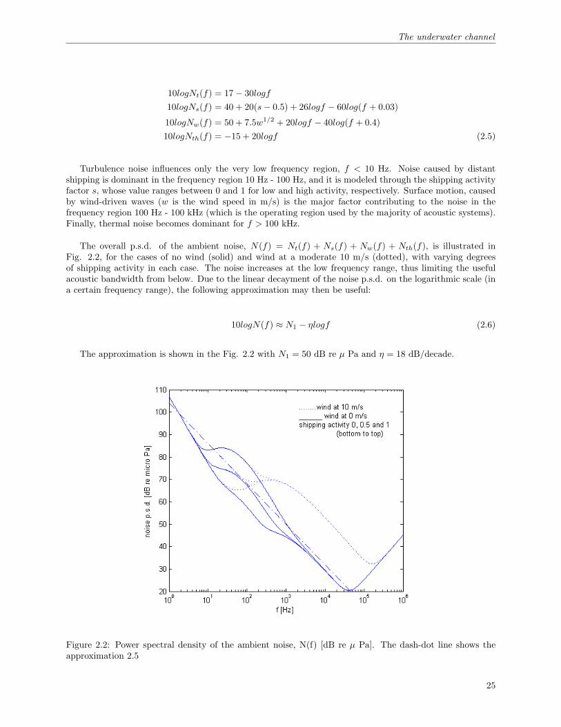
The ambient noise in the ocean can be modeled using four sources: turbulence, shipping, waves, and thermalnoise. The majority of the ambient noise sources can be described by Gaussian statistics and a continuouspower spectral density (p.s.d.). The following empirical formulae give the p.s.d. of the four noise componentsin dB re µ Pa per Hz as a function of frequency in kHz [3]:
24
The underwater channel
10logNt(f) = 17− 30logf10logNs(f) = 40 + 20(s− 0.5) + 26logf − 60log(f + 0.03)
10logNw(f) = 50 + 7.5w1/2 + 20logf − 40log(f + 0.4)10logNth(f) = −15 + 20logf (2.5)
Turbulence noise influences only the very low frequency region, f < 10 Hz. Noise caused by distantshipping is dominant in the frequency region 10 Hz - 100 Hz, and it is modeled through the shipping activityfactor s, whose value ranges between 0 and 1 for low and high activity, respectively. Surface motion, causedby wind-driven waves (w is the wind speed in m/s) is the major factor contributing to the noise in thefrequency region 100 Hz - 100 kHz (which is the operating region used by the majority of acoustic systems).Finally, thermal noise becomes dominant for f > 100 kHz.
The overall p.s.d. of the ambient noise, N(f) = Nt(f) + Ns(f) + Nw(f) + Nth(f), is illustrated inFig. 2.2, for the cases of no wind (solid) and wind at a moderate 10 m/s (dotted), with varying degreesof shipping activity in each case. The noise increases at the low frequency range, thus limiting the usefulacoustic bandwidth from below. Due to the linear decayment of the noise p.s.d. on the logarithmic scale (ina certain frequency range), the following approximation may then be useful:
10logN(f) ≈ N1 − ηlogf (2.6)
The approximation is shown in the Fig. 2.2 with N1 = 50 dB re µ Pa and η = 18 dB/decade.
Figure 2.2: Power spectral density of the ambient noise, N(f) [dB re µ Pa]. The dash-dot line shows theapproximation 2.5
25

The underwater channel
2.1.3 Propagation delay
The experienced delays in an underwater acoustic communication link are much higher than in an open-air link. The nominal speed of sound in water is 1,500 m/s, which is 200,000 lower than the speed ofelectromagnetic waves in open-air (3,000·105 m/s). This causes long propagation delays, which becomes amajor complication for the application of feedback to correct the channel distortions. As an example, typicalpropagation delays in acoustic underwater links can be of several seconds, while the measured coherence timein an underwater channel can be of 100 milliseconds. In contrast with the propagation delays in underwaterchannels, the open-air propagation delay is typically of some microseconds.
2.1.4 Multipath
Multipath propagation is one of the common problems in communications through underwater acoustic links.This propagation phenomenon results in communication signals reaching the receiving antenna by two ormore paths. At the receiver, due to the presence of multiple paths, more than one pulse will be received,and each one of them will arrive at different times. Thus, the channel impulse response will be expressed by:
h(t) =N∑p=1
hpδ(t− τp) =N∑p=1
ρpejφpδ(t− τp) (2.7)
where the channel taps, hp, arriving at τp, can be described by an amplitude component ρp and a phaseshift φp.
Underwater multipath can be caused either by reflection or refraction of the acoustic waves. Reflectionof the acoustic waves occurs when the wave bounces either at the surface or the bottom and reaches thereceiver. It is most common in shallow water environments. Refraction of the communication waves isa typical phenomenon in deep water links, where the speed of sound changes at different depths. Anexplanatory scheme is shown in Fig. 2.3.
Figure 2.3: Multipath effects. Reflective effects (dashed line) and refractive effects (dotted line)
The distortions caused by multipath must be equalized in the receiver. In addition, ways to avoid Inter-Symbol Interference (ISI) must be designed in order to correctly demodulate and detect the transmitteddata. Later on in Chap. 6 a receiver algorithm for underwater acoustic channels that deals with multipatheffects will be explained.
26

The underwater channel
2.1.5 Doppler effect
Another common problem of underwater acoustic communication systems is the fact that they have to dealwith a non-negligible Doppler effect of the acoustic waves. The Doppler effect is caused by the relativemotion of the transmitter-receiver pair, and it causes a shift in the frequency components of the transmittedsignal. The frequency shift is mainly described by the factor vr/c, where vr is the relative velocity betweentransmitter and receiver, and c is the signal propagation speed (the speed of sound underwater in this case).In underwater environments c is much lower than in open-air, and so the Doppler effect is not ignorable. Inaddition, the fact that underwater systems are wideband causes much different Doppler shifts for differentfrequency components of the transmitted signal. This is typically known as frequency spreading.
It is of key importance that underwater acoustic systems deal with non-uniform Doppler effect. As anexample, a bad Doppler effect correction in a multicarrier system could cause Inter-Carrier Interference (ICI),which happens when some distortion due to other subcarriers’ information is present in a selected channel.Although no Inter-Carrier Interference compensation technique has been considered necessary in this study,further information can be found in [4].
2.2 Resource allocation
Taking into account the physical models of acoustic propagation loss and ambient noise, the optimal frequencyallocation for communication signals can be calculated. Considering optimal signal energy allocation, suchfrequency band is defined so that the channel capacity is maximized [5, 6].
The results that are assessed suggest that, despite the frequency spectrum is not yet regulated by theFederal Comission of Communications (FCC) for underwater acoustic communications, the possibilities interms of usable frequency bands are not numerous, due to acoustic path propagation and noise characteristics.
2.2.1 The AN product and the SNR
The narrow-band Signal to Noise Ratio (SNR) observed at a receiver over a distance l when the transmittedsignal is a tone of frequency f and power P is given by
SNR(l, f) =P/A(l, f)N(f)∆f
=S(f)
N(f)A(l, f)(2.8)
where ∆f is a narrow band around the frequency f , and S(f) is the power spectral density of thetransmitted communication signal. Directivity indices and losses other than the path loss are not counted.The AN product, A(l, f)N(f), determines the frequency-dependent part of the SNR. The inverse of the ANproduct, 1/A(l, f)N(f), is illustrated in Fig. 2.4.
2.2.2 Optimal frequency
Observing the inverse of the AN product, 1/A(l, f)N(f) (Fig. 2.4), it can be concluded that for each distancel there clearly exists an optimal frequency f0(l) for which the maximal narrow-band SNR is obtained at thereceiver. The optimal frequency is plotted in Fig. 2.5 as a function of the transmitter-receiver distance.
27

The underwater channel
Figure 2.4: Frequency-dependent part of the SNR, 1/A(l, f)N(f). Practical spreading, k = 1.5, is used forthe path loss A(l, f). The linear approximation is used for the noise p.s.d. N(f)
Ideally, when implementing a communication system, some transmission bandwidth around f0(l) is cho-sen. The transmission power is adjusted so as to achieve the desired SNR level throughout the selectedfrequency band. Practically, the response of the transducers and hydrophones must be taken into accountand the optimal transmission frequency may vary.
2.2.3 3 dB bandwidth definition
A common definition for the system bandwidth in communications is the 3 dB bandwidth one. We definethe 3 dB bandwidth B3dB(l) as that range of frequencies around the optimal frequency f0(l) for whichSNR(l, f) > SNR(l, f0(l))/2. From (2.8) and considering a constant p.s.d. of the transmitted signal,S(f), the previous relation can be expressed as A(l, f)N(f) < 2A(l, f0(l))N(f0(l)) = 2ANmin(l). The 3 dBbandwidth, B3dB(l), and the center frequency of the frequency band, fc(l), are shown in Fig. 2.5. Similartrends are observed for these two parameters and the optimal frequency, f0(l), as it is expected.
2.2.4 Transmission power
Once the transmission bandwidth is set, the transmission power P (l) can be adjusted to achieve a desirednarrow-band SNR level corresponding to the 3 dB bandwidth B3dB(l). If we denote by Sl(f) the p.s.d. ofthe transmitted signal chosen for the distance l, then the total transmitted power is
28

The underwater channel
Figure 2.5: Optimal frequency f0(l) considering the inverse of the AN product, 1/A(l, f)N(f). The 3 dBbandwidth, B3dB(l), and the center frequency of this bandwidth, fc(l), is also shown
P (l) =∫B3dB(l)
Sl(f)df = SNR0B3dB(l)
∫B3dB(l)
N(f)df∫B3dB(l)
A−1(l, f)df(2.9)
where the transmitted signal p.s.d. is considered constant in the signal bandwidth.
As a practical impact of the center frequency, fc(l), and the transmission bandwidth to the requiredtransmission power for the successful reception of communication signals, some experimental results areshown in Fig. 2.6.
29

The underwater channel
Figure 2.6: Required transmission power for quiet measurements in an oil field
30

Chapter 3
Video compression techniques
In the realm of video compression, better visual quality with higher compression rates are the main goalsthat must be met by the techniques to be successful in the marketplace. In the underwater channel, thetransmission link has a limited bit rate capacity, which can be of about tenths of kbps (typical bit ratesare 10-30 kbps). This fact makes it even more important to find powerful compression techniques that canreduce the requirements for real-time video transmissions. For instance, a very low resolution video (QCIF)with a frame rate of about 5 fps will require about 1.5 Mbps for its uncompressed transmission. Even in thiscase, a compression factor of about 1:100 is needed to achieve the targeted reduction in data rate.
Today, compression methods exist that can be used to transmit video at 64 kbps. In particular, thecommercially-available MPEG-4 encoders provide compression at this rate, by combining spatial and tempo-ral techniques. Existing efforts at applying MPEG-4 compression for acoustic underwater video transmissioninclude [7], where a single carrier modulation scheme operates over a short range (300 m).
3.1 Compression fundamentals
3.1.1 Images and video
To understand how a compression technique works, a few words must be said about common concepts suchas image and video. In the image processing field, an image is considered to be a two-dimensional arrayof samples that are called pixels (picture elements, Fig. 3.1). Each picture element can be a vector of anydimension that represents the visual information that it contains. It can be just a one-dimensional vectorwhich represents luminance (or luminous intensity) for grey-scale images, or three-dimensional vectors whichrepresent color components for color images.
Many techniques have been designed to accurately represent color images. The easiest one, but less used,is the RGB (Red Green Blue) components system, in which an image is represented by 3 vectors, each ofwhich containing the intensity of red, green and blue that the image has.
Another popular way to represent the color images is using the YUV space components system, where animage is defined by its luminance Y, and two color difference components (U,V). These two color differencecomponents are defined as U=B-Y and V=R-Y. The main advantage of this representation system is thatgrey-scale images can be represented by black and white devices by just choosing the Y component. Inaddition, the human visual system is more sensitive to luminance than color, and using this representation
31

Video compression techniques
Figure 3.1: Image pixels
a higher resolution can be given to the Y component despite sacrificing some resolution for color differencecomponents (U,V). An example image decomposition is shown in Fig. 3.2.
Figure 3.2: YUV image representation. (1) Original signal. (2) Luminance Y signal. (3) Chrominance Vsignal. (4) Chrominance U signal
The quality of an uncompressed digital picture depends on two important parameters: resolution (width× height) and color depth (number of bits used to represent each pixel). The picture is finer with higherresolution, or in other words, more pixels are used. As a result, the edges become smoother and theimage more natural. Some standard resolutions include 1920×1080 for full high definition television systems(HDTV) or 640×480 for conventional VGA systems. Typical color depths are 1 bit (2 colors), 8 bits (256colors), 16 bits (65536 colors), 24 bits (true color), etc.
A video consists of a sequence of still images that are captured from a recording device and that, correctlytimed and displayed, convey not only the picture information, but also the motion in a scene (Fig. 3.3).
Some words must be said about the timing of the individual images in a video. Nowadays time-stampsare transmitted to accurately indicate the exact moment when an image should be displayed, so that thetargeted frame rate is achieved. The frame rate in a video is another quality measurement as from it dependsthe subjective motion sensation. With higher frame rate the motion becomes smoother but it requires thetransmission of more data, as more images are sent for each second of video. It is well known that about 25fps are required to correctly show the motion in a general purpose video, although a lower frame rate might
32

Video compression techniques
Figure 3.3: Consecutive images of a video file
be used for low motion sequences. Fortunately, underwater video imagery can be included in this last group,and even some images each 5 or 10 seconds may suffice for some applications.
3.1.2 Compression approaches
Video compression becomes possible since there are mainly two types of redundancies: spatial and temporal.Spatial redundancy exists between nearby regions of an image where the color components don’t changemuch. Temporal redundancy exists as, given a proper frame rate, there is not much change between a frameand the next. There are two basic approaches to video compression, depending on what type of redundancywithin the video sequence is exploited.
In the first approach, video is treated as a sequence of independent images, each of which is individuallycompressed and transmitted over the channel (intra mode). This approach has been favored in almost allexisting attempts at video transmission over underwater acoustic channels [8–13].
The majority of these efforts used the standard JPEG compression, which is based on the Discrete CosineTransform (DCT). Its basic steps are the following:
1. Division of the image into blocks (usually 8x8 pixel blocks) (see Fig. 3.4)
Figure 3.4: Division of the image into blocks
2. Every block is compared to the DCT basis (see Fig. 3.5)
In the second approach, the images in a video sequence are not encoded independently. Instead, only thefirst image in a sequence is fully encoded, while from there on, the difference between successive images isencoded. Since the images do not change rapidly, their difference can be represented by fewer bits than thefull image, and, hence, the required bit rate can be reduced.
33

Video compression techniques
Figure 3.5: Image (left) and DCT basis (right)
The practical implementations include the transmission of motion vectors that represent the motion inthe scene, along with the prediction error after the application of the calculated motion vectors (inter mode).The transmission of the prediction error is necessary to avoid error propagation in the receiver. A transmitterscheme is shown in Fig. 3.6.
Figure 3.6: Temporal coding transmission scheme
The best performance for motion compensation algorithms is achieved when a combination of forwardpredicted pictures from a past image, and bi-directional predicted pictures from both a past image and afuture image is transmitted.
The main drawback of temporal coding is the error propagation. Due to that, the standards define theGroup Of Pictures (GOP), which include Intra frames (which do not depend on other images), forwardpredicted frames (P frames), and bi-directional predicted frames (B frames). A sample GOP is shown inFig. 3.7.
Figure 3.7: Group Of Pictures (GOP)
34

Video compression techniques
3.2 MPEG-4 standard
Moving Picture Experts Group (MPEG) is an experts group formed by the International Organization forStandardization (ISO) to set standards for audio and video compression and transmission. MPEG standardsconsist of certain Parts that cover different aspects of the specification. The standards also define Profilesand Levels that define a set of tools and parameters for practical systems.
MPEG-4 (1998) provides more complex coding tools and higher compression factors than its predecessorsMPEG-1 and MPEG-2. Its main feature is the definition of the concept Audio-Visual Object (AVO), orientedto manipulation.
3.2.1 Functionalities
MPEG-4 was initially designed for audiovisual encoding at very low bit rates (< 64 kbps, 64 - 384 kbps, 384kbps - 4 Mbps) with attention to error resilience. Later on, its focus shifted to an object oriented approach,with multiple audiovisual objects encoded using different techniques and composited in the decoder.
It uses a hybrid temporal-spatial coder (basic scheme shown in Fig. 3.8) for natural and synthetic datacoding, with improved temporal random access and coding efficiency, and high robustness in challengingenvironments.
Figure 3.8: Hybrid temporal-spatial coding basic scheme
3.2.2 Very Low Bit-rate Video core
In the MPEG-4 standard, besides content-based functionalities for modern interactive multimedia systems,there are specified functionalities for very low bit rate video in error prone environments.
As it can be seen in Fig. 3.9,VLBV Core (Very Low Bit-rate Video) provides algorithms and tools forapplications operating at bit rates typically between 5 and 64 kbps. They support image sequences with lowspatial resolution (typically up to CIF resolution) and low frame rates (typically up to 15 Hz). The basicapplications’ specific functionalities supported by the VLBV Core include coding of conventional rectangularsize image sequences with high coding efficiency and high error robustness/resilience, low latency and lowcomplexity for real-time multimedia communication applications.
For the current project, with limited available bit rate due to the characteristics of the underwaterchannel, MPEG-4 VLBV Core is a good candidate.
35

Video compression techniques
Figure 3.9: Classification of the MPEG-4 image and video coding algorithms and tools
3.3 Implementation
The compression method chosen in this project is based on the MPEG-4 Part 2 (Visual) with Simple Profile.
3.3.1 MPEG-4 codec
The popular MPEG-4 Xvid codec is used. Xvid is an open-source research project focusing on video com-pression and is a collaborative development effort. All its code is released under the terms of the GNUGeneral Public License (GPL).
The Xvid video codec implements MPEG-4 Simple Profile and Advanced Simple Profile standards withfeatures such as: B frames, global and quarter pixel motion compensation and lumi masking, among others.It allows compression and decompression of digital video, in order to reduce the required bandwidth of videodata for transmission over computer networks, or efficient storage on CDs or DVDs.
3.3.2 Performance
The performance of the MPEG-4 codec has been tested by compressing two video files, which are the onesthat have been used for the underwater video experiments. The video files have different resolutions, andtwo different compression factors have been chosen, one with high compression for the low resolution file,and the other with lower compression performance for the high resolution video.
Figure 3.10: Lower quality video (left) and higher quality video (right)
36

Video compression techniques
The low quality (LQ) video consists of a rise inspection footage and has been recorded with a resolution of256×256 pixels. Along with the higher compression factor, it represents a quite appropriate set of parametersfor a real-time video transmission.
The high quality (HQ) video is taken from a Titanic shipwreck inspection and has a resolution of 480×320pixels. As an example of a transmission of higher quality video with current techniques, it has been com-pressed with a slightly lower compression factor.
The table 3.1 shows a comparison of different parameters for the modulated videos, along with an assessedreal-time frame rate that could be supported for such files with two sets of realistic modulation parameters.The table 3.2 contains the information about the modulation parameters (1) and (2).
Pipe inspection Titanic footageRecorded video duration (s) 1.67 20
Modulated signal duration (s) with (1) 2.61 42.41Modulated signal duration (s) with (2) 4.14 70.61
Number of frames 50 319Recorded frame rate 30 30
Real-time frame rate (1) 19.16 7.52Real-time frame rate (2) 12.08 4.52
Table 3.1: Frame rate study
Bandwidth (kHz) Subcarrier modulation FEC coding Data rate (kbps)Configuration (1) 115 8-PSK BCH(63,30) 151Configuration (2) 115 8-PSK BCH(63,18) 91
Table 3.2: OFDM system parameters
37


Chapter 4
OFDM fundamentals
Single-carrier equalization [14] is a method that has been used for virtually all systems that attempted imageor video transmission through an underwater acoustic channel. This method has also been used in previouswork done at the MIT Sea Grant College Program [10], where pre-packaged video images were transmittedat a very high bit rate of 150 kbps, but only over a stable, 10 m long vertical path.
Research in the area of underwater acoustic communications over the past several years has resulted indemonstrating a different type of bandwidth-efficient modulation and detection method, which uses multiplecarriers instead of a single carrier. In its basic form, this method is known as Orthogonal Frequency DivisionMultiplexing (OFDM).
Because of its simplicity, OFDM has found application in many wireline (DSL) and wireless radio systems(digital audio and video broadcast, wireless LAN) and is being considered for the fourth generation mobilecellular systems. Its application to underwater acoustic systems has been addressed recently.
4.1 General description
Modulation is the process of transforming a message signal to make it easier to work with. In telecom-munications, signal modulations are chosen taking into account some parameters, such as implementationcomplexity, supported data rate, and robustness against channel and noise effects.
Multi-carrier modulation is an attractive alternative to single-carrier broadband modulation on channelswith frequency-selective distortion. It is based on the idea of dividing the total available bandwidth into manynarrow subbands, such that the channel transfer function appears constant (ideal) within each subband. Bydoing so, the need for time-domain channel equalization is eliminated. Instead, the subbands have to beseparated in the frequency domain, which is efficiently performed using only the Fast Fourier Transform(FFT). This efficient implementation using the FFT can be executed for multi-carrier modulation anddetection when used with rectangular pulse shaping.
The modulation technique on which the project is based is the Orthogonal Frequency Division Multi-plexing (OFDM) scheme and its ability to convey the information modulated in multiple subcarriers using abasic modulation scheme, achieving an adequate transmitter/receiver complexity, appropriate capacity, andproviding numerous possibilities for channel compensation.
OFDM is a frequency-division multiplexing (FDM) scheme utilized as a digital multi-carrier modulation
39

OFDM fundamentals
method. A large number of closely-spaced orthogonal subcarriers are used to carry data. The data is dividedinto several parallel data streams or channels, one for each subcarrier. Each subcarrier is modulated with aconventional modulation scheme (such as Quadrature Amplitude Modulation -QAM- or Phase Shift Keying-PSK-) at a low symbol rate, maintaining total data rates similar to conventional single-carrier modulationschemes in the same bandwidth. Fig. 4.1 shows the utilization of the available bandwidth for a 7 subcarriersOFDM signal.
Figure 4.1: Bandwidth utilization for an OFDM signal
4.2 Orthogonality
One of the main features of OFDM is that the subcarriers are chosen to be orthogonal to each other. Thatmeans that in the center frequency of the subcarrier k, fk, the other subcarriers’ amplitude is null (see Fig.4.1). The consequence of this fact is that cross-talk between subchannels is avoided and inter-carrier guardbands are not necessary. This leads to a simplification of the design for both the transmitter and receiver,as a separate filter for each subchannel is not required (unlike other FDM schemes).
The orthogonality principle requires a subcarrier spacing of ∆f = α/T Hz (as shown in Eq. 4.1), whereT is the useful symbol duration in seconds, and α is a positive integer (typically 1). Hence, the total usefulbandwidth is B = K∆f Hz, where K is the total number of subcarriers.
〈φk(t), φm(t)〉 =∫ T
0
ej2π(k−m)∆ftdt =ej2π(k−m) − 12π∆f(k −m)
= δ(k −m) (4.1)
One of the most important advantages of orthogonality between subcarriers is that it allows high spectralefficiency, as almost the full available frequency band can be utilized.
A disadvantage that results from the use of orthogonality is the need for highly accurate frequencysynchronization between the transmitter and the receiver. The frequency deviation that OFDM systemscan tolerate is very small, as the subcarriers will no longer be orthogonal, causing Inter-Carrier Interference(ICI), or cross-talk between subcarriers.
Frequency offsets are typically caused by Doppler shifts due to motion, or mismatched transmitter andreceiver oscillators. While Doppler shift alone may be compensated for by the receiver, the situation isworsened when combined with multipath, as reflections will appear at various frequency offsets, which ismuch harder to correct.
40

OFDM fundamentals
4.3 Modulation using FFT
Due to the orthogonality of OFDM subcarriers, the modulator and demodulator can be efficiently imple-mented using the FFT algorithm on the receiver side, and the inverse FFT, or IFFT, on the transmitter side.As it has been claimed, on the transmitter side the IFFT of a signal X(k), where k denotes the frequencycomponent index, is
x(l) =1K
K−1∑k=0
X(k)ej2πkl/K , l = 0, ...K − 1 (4.2)
where K designates the number of frequency components, and x(l) is the resulting sampled signal, whichis formed by the sum of the modulated frequency components X(k) (at their corresponding digital frequencyk/K). To retrieve again the digital frequency components, the inverse equation must be used:
X(k) =K−1∑l=0
x(l)e−j2πkl/K , k = 0, ...K − 1 (4.3)
which corresponds to the K-point FFT of X(k).
The transmission side is shown in Fig. 4.2, where an IFFT applied to the subcarrier complex constellationpoints is enough to assess the time domain sequence. A complementary receiver is easily implemented byperforming an FFT on the received modulated signal, retrieving the complex symbols for each subcarrier.
Figure 4.2: Efficient transmitter implementation using IFFT
4.4 Guard time
One of the advantages of the OFDM scheme is that, since the data in each block is divided into K parallelsymbol streams that are transmitted at a low symbol rate, the system may become more robust againstInter-Symbol Interference (ISI) caused by the multipath channel.
As the duration of each symbol is longer than in a single high rate stream, the insertion of a guardtime between the OFDM blocks (or symbols) is feasible, thus reducing the possible ISI. In addition, theguard interval also eliminates the need for a pulse-shaping filter, and it reduces the sensitivity to timesynchronization problems.
41

OFDM fundamentals
4.5 Equalization
The need for highly complex time domain equalizers is avoided in OFDM system implementations. Thefact that a number K of narrow-band channels is used to deliver the symbols helps mitigate the effects offrequency-selective channel conditions, such as fading caused by multipath propagation. Within a subcarrierband the channel is considered constant (flat) if the number of subcarriers K is large enough, hence makingchannel equalization far simpler than in single-carrier systems.
If differential detection or differential modulation (such as DPSK or DQPSK) is applied to the subcarriers,equalization can be completely omitted, since these non-coherent schemes are insensitive to slowly changingamplitude and phase distortion.
4.6 Advantages
The main advantage of the OFDM modulation scheme in terms of practical implementation is that it enableschannel equalization in the frequency domain, thus eliminating the need for potentially complex time-domainequalizers.
OFDM modulation techniques have been used both in wired and wireless systems due to its advantages.Among them, the following must be mentioned:
• Simple and effective channel equalization in the frequency domain
• High spectral efficiency
• Robustness against Inter-Channel Interference (ICI)
• Robustness against Inter-Symbol Interference (ISI) and fading caused by the multipath channel
• Efficient implementation using the FFT, avoiding the need for complex subchannel filters
• Low sensitivity to time synchronization errors
4.7 Disadvantages
The major disadvantages of OFDM are:
• Sensitivity to frequency offsets
• High Peak to Average Ratio (PAR), with a subsequent difficulty to optimize the transmission power
The major difficulty in applying OFDM to an underwater acoustic channel is the signal’s sensitivity tofrequency offsets, which imposes strict synchronization requirements. Motion-induced Doppler effect in anacoustic channel creates a frequency offset that is not uniform across the signal bandwidth. This fact is instark contrast to the frequency distortion in radio systems, and, hence, many of the existing synchronizationmethods cannot be used directly. Instead, dedicated methods have to be designed. Such methods havebeen proposed over the past several years, and demonstrated good performance in initial trials with realdata transmitted over a few kilometers at bit rates on the order of 10 kbps within comparable acousticbandwidths [15–17].
42
Chapter 5
OFDM transmitter
One of the most important parts of the project is designing a concrete system that can reach the desiredperformance under experimental conditions. To do so, some practical considerations must be taken intoaccount and, given that information, the implementation is then designed to best perform with the availablehardware.
The implemented OFDM system is defined in this chapter, and the chosen system model is introduced.In addition, the different implementation parts are explained.
5.1 System model
The model used on the transmitter side consists of a typical OFDM system with K subchannels, where theinput data stream (in the video case, the MPEG-4 coded video file) is scrambled to uniformize the powerallocation and randomize the values “0” and “1” in the input data stream. After that, the channel codingis performed and the data stream that comes out of the coder is serial-to-parallel converted into K streamsdk(n), k = 0, ...K − 1. These streams are then interleaved and used to form the signals
uk(t) =∑n
dk(n)ejk∆ω(t−nT ′)g(t− nT ′) (5.1)
where the following apply:
• The signal g(t) is a rectangular pulse in time with unit amplitude and duration T
• T ′ = T + Tg, where Tg is the guard interval, which is longer than the multipath spread
• ∆ω = 2π∆f , where ∆f = 1/T is the carrier spacing
The synchronization preamble in baseband and the guard times are included to the signal∑K−1k=0 uk(t)
to create the signal z(t), and then a frequency shift is applied so that the modulated signal is given by
s(t) = Re{z(t)ejω0t} (5.2)
43
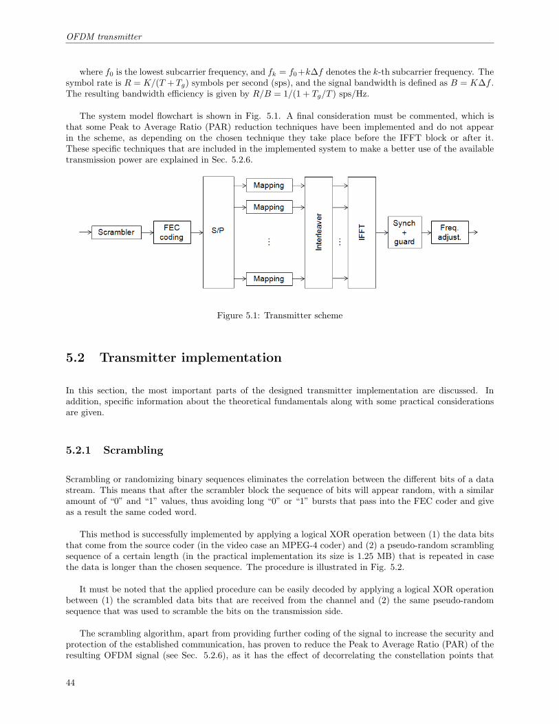
OFDM transmitter
where f0 is the lowest subcarrier frequency, and fk = f0+k∆f denotes the k-th subcarrier frequency. Thesymbol rate is R = K/(T +Tg) symbols per second (sps), and the signal bandwidth is defined as B = K∆f .The resulting bandwidth efficiency is given by R/B = 1/(1 + Tg/T ) sps/Hz.
The system model flowchart is shown in Fig. 5.1. A final consideration must be commented, which isthat some Peak to Average Ratio (PAR) reduction techniques have been implemented and do not appearin the scheme, as depending on the chosen technique they take place before the IFFT block or after it.These specific techniques that are included in the implemented system to make a better use of the availabletransmission power are explained in Sec. 5.2.6.
Figure 5.1: Transmitter scheme
5.2 Transmitter implementation
In this section, the most important parts of the designed transmitter implementation are discussed. Inaddition, specific information about the theoretical fundamentals along with some practical considerationsare given.
5.2.1 Scrambling
Scrambling or randomizing binary sequences eliminates the correlation between the different bits of a datastream. This means that after the scrambler block the sequence of bits will appear random, with a similaramount of “0” and “1” values, thus avoiding long “0” or “1” bursts that pass into the FEC coder and giveas a result the same coded word.
This method is successfully implemented by applying a logical XOR operation between (1) the data bitsthat come from the source coder (in the video case an MPEG-4 coder) and (2) a pseudo-random scramblingsequence of a certain length (in the practical implementation its size is 1.25 MB) that is repeated in casethe data is longer than the chosen sequence. The procedure is illustrated in Fig. 5.2.
It must be noted that the applied procedure can be easily decoded by applying a logical XOR operationbetween (1) the scrambled data bits that are received from the channel and (2) the same pseudo-randomsequence that was used to scramble the bits on the transmission side.
The scrambling algorithm, apart from providing further coding of the signal to increase the security andprotection of the established communication, has proven to reduce the Peak to Average Ratio (PAR) of theresulting OFDM signal (see Sec. 5.2.6), as it has the effect of decorrelating the constellation points that
44

OFDM transmitter
Figure 5.2: Scrambler scheme
come out from the subcarrier mapper. An example of its effect is shown in Fig. 5.3, where the first peakpresent when scrambling is not used is eliminated in the case it is enabled.
Figure 5.3: Scrambling effect on PAR reduction: (left) OFDM sample block with non-scrambled bits, and(right) OFDM sample block with scrambled bits
5.2.2 FEC coding
The long packet delays due to the low speed of propagation in underwater environments suggest the avoidanceof packet retransmissions due to errors. Given the conditions of the channel, the inclusion of Forward ErrorCorrecting (FEC) codes is strongly necessary given the conditions of the channel, as they provide errorcorrection capability and avoid such critical circumstances.
FEC coding is a system of error control for data transmission, whereby the transmitter adds redundantdata to its messages, so that a specific amount of random errors in the received bit sequences can successfullybe corrected by the decoder. To make best use of the FEC coder, the possible error bursts due to momentarybad channel conditions or highly attenuated frequency bands must be minimized, and that is why the systemmust also include an interleaver block.
The channel coding field is a very active one, as there is a two-fold approach when designing an appropriatecoding technique: first, it has to provide the desired error correction capability, and second, it has to provide
45

OFDM transmitter
enough coding and decoding speed so as not to affect the transmission timing. There are different types ofcoders depending on the implementation:
1. Block codes: this family of codes work on fixed-size blocks (packets) of bits or symbols of predeterminedsize. Practical block codes can generally be decoded in polynomial time to their block length.
2. Convolutional codes: this family of codes work on bit or symbol streams of arbitrary length. They aremost often decoded with the Viterbi algorithm, though other algorithms are sometimes used. Viterbidecoding allows asymptotically optimal decoding efficiency with increasing length of the convolutionalcode, but at the expense of exponentially increasing complexity.
As it has been mentioned above, there are numerous types of codes. Some of the most popular includethe BCH (Bose, Ray-Chaudhuricodes and Hocquenghem code), which are known by its decoding ease, theLow Density Parity Check (LDPC) codes, which are highly-efficient block codes, and the Turbo codes, thatcombine multiple convolutional codes and an interleaver to produce a block code.
The type of error correcting code (ECC) that has been chosen is the BCH code, due to the followingfacts: its coding and decoding efficiency, the fact that it has been used in previous successful OFDM systemimplementations for underwater environments, and the implementation ease as it comes in a MATLABbuilt-in package.
The BCH codes are polynomial codes over a finite field with a particularly chosen generator polynomialfrom which the codewords are produced. It is also a cyclic code. These codes are multiple error correctingcodes and a generalization of the Hamming codes.
The codewords are formed by taking the remainder after dividing a polynomial representing the informa-tion bits by a generator polynomial. The generator polynomial is selected to give the code its characteristics.All codewords are multiples of the generator polynomial [18].
For the practical implementation, a set of BCH codes with different redundancies and error capabilityhas been tested. The characteristics of these codes are summarized in Tab. 5.1. Different channel utilizationis possible depending on the chosen code, as the implementation allocates an integer number of codewordsin each OFDM block for direct demodulation and decoding.
The ratio that assesses the channel utilization given a BCH code is N/(N + 1), where N is the codewordlength of the specific code. The system is designed so that K/(N + 1), where K is the total number ofsubcarriers, is an integer. This ratio also represents the number of subcarriers that are not used, which areequispaced and may be used to carry pilots.
BCH code7/4 15/11 31/21 63/51 63/30 63/18 63/10 127/120 255/239
Coding ratio 1.75 1.36 1.48 1.24 2.10 3.50 6.30 1.06 1.07Ch. utilization (%) 88 94 97 98 98 98 98 99 100Correction (bits) 1 1 2 2 6 10 13 1 2
Table 5.1: BCH coding characteristics
To test the behavior of the selected codes, some Additive White Gaussian Noise (AWGN) has beenartificially added to generated OFDM signals and the decoded Bit Error Rate (BER) has been evaluatedand contrasted with theoretical curves (with positive matches). The results are shown in Fig. 5.4.
In practical experiments, the most appropriate BCH code has to be chosen by evaluating the achieved
46

OFDM transmitter
Figure 5.4: Decoded BER vs. SNR for an OFDM system with K=16384, 8-PSK subcarrier modulation, andAWGN
BER results for different coding ratios, such that the code with minimal redundancy that achieves a targeteddecoding performance is selected (as illustrated in Sec. 8.3.2).
5.2.3 Subcarrier mapping
The modulations chosen in the current research to modulate the subcarriers are the Quadrature AmplitudeModulation (QAM) and the Phase Shift Keying (PSK) ones.
1. Phase Shift Keying (PSK) is a digital modulation scheme that conveys data by changing, or modulating,the phase of a reference signal (the carrier wave). The constellation points chosen are usually positionedwith uniform angular spacing around a circle.
These PSK types have been implemented (see constellation points in Fig. 5.5):
• Quadrature PSK (QPSK): Circle constellation of 4 points with 2 bits assigned to each point.
• 8-PSK: Circle constellation of 8 points with 3 bits assigned to each point.
Note that when differential detection is performed, the PSK mapped points are further processedto retrieve the transmitted constellation, including a 45◦ shift of the QPSK constellation, which isnecessary to mantain the 4 points constellation (for more details on the differential detection algorithmand the transmitter modifications see Sec. 6.5.1).
2. Quadrature Amplitude Modulation (QAM) is a digital modulation scheme that conveys data by chang-ing, or modulating, both amplitude and phase of a reference signal. It is usually implemented as twoamplitude modulation schemes for two added carriers, which are out of phase with each other by 90◦.
These QAM types have been implemented (see constellation points in Fig. 5.6):
47

OFDM transmitter
Figure 5.5: PSK modulation constellations
• 16-QAM: Squared constellation of 16 points with 4 bits assigned to each point.
• 32-QAM: Non-squared constellation of 32 points with 5 bits assigned to each point.
• 64-QAM: Squared constellation of 64 points with 6 bits assigned to each point.
Figure 5.6: QAM modulation constellations
In practice, as higher is the density of points in the constellation, higher is the probability that thesymbols are wrongly detected in the receiver due to the phase shift and amplitude scaling of the complexpoints after passing through the channel. That is why the performance of the different modulation typesmust be tested in the real conditions and appropriate constellations must be chosen (as shown in Sec. 8.3.3).
5.2.4 Frequency interleaving
As it has been stated in the previous section, the error correction capability of channel coding techniquesis optimized when combined with interleaving. In this case, the interleaving is performed in the frequencydomain, across the K subcarriers. The concept of interleaving is graphically shown in Fig. 5.7.
The objective of the interleaving scheme is to separate as much as possible the different parts of acodeword (in this case the bits corresponding to the symbols in each subcarrier) in the frequency domain. Itaims at reducing the impact of highly attenuated or distorted frequency bands due to channel characteristicssuch as multipath propagation or in-band noise, hence avoiding error bursts within a single codeword.
48

OFDM transmitter
Figure 5.7: Interleaving concept. The data carriers are shown in different colors and the P channels representpilots
Figure 5.8: Interleaving matrix and interleaving depth
49

OFDM transmitter
In the implemented system, the interleaving depth δ (see Fig. 5.8), given in number of subcarriers, maybe assessed from the following equation:
δ = K · N
(N + 1) · nd(5.3)
where K is the total number of subcarriers, N is the codeword length, and nd is a factor that indicatesa certain number of symbols, that corresponds to an integer number of codewords. This last parameter ischosen in accordance to the detection algorithm, so that the symbol decision is optimized.
As a practical example, the designed interleaving depth δ for a system with K = 16384 subcarriers thatuses a BCH(63,18) code is δ = 256 subcarriers. Considering a bandwidth of 115 kHz, it corresponds to afrequency band of 1.8 kHz.
5.2.5 IFFT modulation
Once the mapped subcarriers’ symbols are interleaved, the OFDM temporal blocks are assessed using theIFFT algorithm. Despite it having been discussed in Sec. 4.3, a final consideration must be made about thepractical implementation of this procedure.
As it may be expected, some oversampling is required in order to assure the correct demodulation of theOFDM blocks. According to the Nyquist sampling theorem, the sampling frequency, fs, must accomplishthe relation fs > 2fh, where fh is the highest frequency component of the transmitted signal. In this case,fh is the highest frequency of the band-pass signal (after frequency adjustment, see Sec. 5.2.8).
In the practical case, further oversampling is recommended due to the inherent complexity of underwatercommunications, and an oversampling ratio of between 3 and 4 is advised.
To correctly count for the oversampling, the IFFT algorithm does not operate with a number of samples K(the total number of subcarriers), but it operates with a number of samples γK, where γ is the oversamplingratio, and (γ − 1)K zeros have been appended to the K subcarriers’ symbols.
Thus, the IFFT algorithm performs the following equation:
y(l) =Ns−1∑k=0
d(k)ej2πkl/Ns , l = 0, ..., Ns − 1 (5.4)
where Ns is the number of samples during a symbol time, given by Tfs, and d(k) is a vector of Nssamples, which contains the subcarriers’ symbols in the first K positions, and the (γ − 1)K appended zeros.The previous equation is efficiently calculated by multiplying the Ns-point IFFT of d(k) by Ns.
5.2.6 Peak to Average Ratio reduction
One of the major disadvantages in OFDM systems is its inherent difficulty to control the signal amplitude inthe time domain. As the waveform shape is determined by the output of the IFFT applied to the subcarriers’symbols, which at the same time depend on the sequence of bits from the FEC coder (see Fig. 5.1), theshape of the signal can vary considerably from block to block.
50

OFDM transmitter
The main consequence of this block-to-block variation is the existence of peaks in the signal that establisha limit in the maximum power of the transmitted signal. In other words, the peaks are transmitted at themaximum power and the rest of the signal is transmitted at a much lower power.
One of the possible suboptimal solutions for this problem is to assume a certain in-band distortion causedby the non-linear response of the chosen power amplifier. In this case, the amplifier input voltage is definedso that the peaks of the signal are transmitted with slightly higher power than the limit of the linear regionof operation, thus gaining some power, but introducing distortion.
The present distortion is due to intermodulation products among subcarriers, and causes spectral growthof the multicarrier signal. As a result, the frequency synchronization is affected, and, as it has been previouslycommented, OFDM systems are very sensitive to these maladjustments.
Because of the importance of such issue in OFDM implementations, and being even more critical inunderwater communications (where the attenuation caused by the channel is higher than in radio environ-ments, and the signal amplitude is too weak), the reduction of the signal variation through time is a veryactive field of research. Such variation can be evaluated by the Peak to Average Ratio (PAR). The conceptof PAR reduction is illustrated in Fig. 5.9.
Figure 5.9: PAR reduction idea: original OFDM signal (left), and PAR reducted OFDM signal (right), usingthe symbol interleaving technique
The PAR of a signal is defined as the ratio between the maximal power of the signal and its averagepower, as
PAR =max0≤t<T |s(t)|2
1T
∫ T0|s(t)|2dt
(5.5)
where s(t) is the transmitted OFDM signal, and T is the symbol duration time. The PAR is alsocommonly given in dB, as 10log(PAR).
Numerous techniques to reduce this ratio have been proposed in the last years. Some of the most popularones are: clipping and filtering, symbol interleaving, in-band tone reservation, and out-of-band tone insertion.
All the previously mentioned techniques have been included in the current OFDM system, and theresulting PAR has been evaluated. In the following subsections these techniques are discussed, and itsperformance is tested and quantized.
51

OFDM transmitter
Clipping and filtering
The simplest technique that can be used to limit the PAR of a signal is the clipping and filtering technique. Itis based on an amplitude clipping of the signal samples that are over a certain chosen threshold. The sampleswhose amplitude exceeds that threshold are clipped and the amplitude set to the maximum amplitude level,as
s(t) ={
s(t) if |s(t)| ≤ AA · ejarg(s(t)) if |s(t)| > A
(5.6)
The effects of the clipping are not only the reduction of the PAR, but a quantizable in-band and out-of-band distortion is introduced in the signal due to the variation of the signal in the time domain. It is atthis point that filtering is advised to avoid the out-of-band distortion, so that no power is wasted by thehardware components.
Fig. 5.10 shows the implementation that has been selected. In it, the clipping is followed by a band-passFinite Impulse Response (FIR) filter that effectively attenuates the components which are located outsidethe operational frequencies. A similar implementation and performance study is shown in [19]. Some otherpossible implementations include IFFT/FFT blocks to perform the filtering.
Figure 5.10: Clipping and filtering block diagram
Both the clipping threshold and the filter have been chosen according to practical tests, for which theperformance of the detection algorithm has been tested for different filter type/parameters and clippingthreshold values. Some of the selected parameters are summarized in Tab. 5.2.
Filter type FIROrder 128
Gain at WN (dB) -6Clipping threshold (%) 0.002
Table 5.2: Clipping and filtering parameters
The parameter WN is used to represent the edges of the pass band, and the clipping threshold is definedas the percentage of samples that are clipped among the total number of samples of the OFDM signal. Noamplitude value has been established as OFDM signals can vary, and the distortion that can be tolerated iscorrectly limited using the implemented solution.
Symbol interleaving
The high correlation in the subcarriers’ symbols that are used as input for the IFFT block has been demon-strated to cause high PAR signals. Due to that, several techniques have been designed so as to decorrelate
52

OFDM transmitter
the complex points that have a direct impact on the time-domain shape of the signal. One of the mosteffective is the symbol interleaving technique.
In this technique, a set of M interleavers is used to reorder the symbols that are sent to the IFFTmodulator. Given the K symbols that modulate the subcarriers, X = [X0, X1, ..., XK−1], a one-to-onerearrangement, {n} ↔ {π(n)} where π(n) ∈ {0, 1, ...,K − 1}, results in the interleaved symbols, X =[Xπ(0), Xπ(1), ..., Xπ(K−1)] (Fig. 5.11 illustrates the concept). This procedure is performed for each inter-leaver, and hence the sequence with a lower PAR is selected for transmission [20].
Figure 5.11: Symbol interleaving technique
One of the major concerns of this implementation has to do with the generation of the interleavers. Aseach OFDM signal is different, there is no exact method to know which kind of combinations will result inlower PAR. That is why M randomly generated combinations are used, being M a parameter that has tobe set taking into account the practical performance of the system (in this case 32 interleavers has provedto provide enough improvement).
Another issue is the side information that should be transmitted to let the receiver know which interleaverhas been used for each OFDM symbol. This problem is avoided in the current research project by usingpilot symbols in each OFDM block (despite increasing the processing complexity).
The algorithm in reception calculates the Medium Square Error (MSE) between the pilot symbols thatare retrieved from each interleaver and the transmitted pilot symbols (a parameter that is known by thereceiver as it is set prior to transmission). Then, the receiver selects the interleaver that provides a lowerMSE, as it is shown in Fig. 5.12.
Other possible interleaving implementations include the bit interleaving technique, where the bits, insteadof the mapped symbols, are used as an input for the interleaving algorithm [20].
In-band tone reservation
As it has been commented in the previous sections, the OFDM signal peaks are a direct consequence ofthe symbols used to modulate the transmitted signal. Thus, the rearrangement of these symbols (as in theinterleaving method) successfully provides a PAR reduction to the OFDM signal if an appropriate change ismade.
The in-band tone reservation technique aims at modifying the shape of the time-domain signal by selectingthe symbols that will be transmitted on several subcarriers [21, 22], so that the PAR of the resulting OFDMsignal is reduced. The main idea is quite similar to the previous technique’s one in the sense that it makes
53
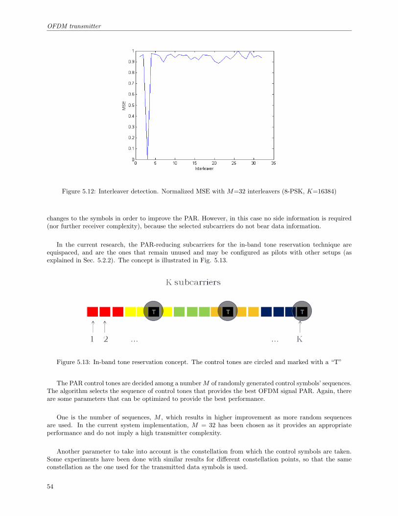
OFDM transmitter
Figure 5.12: Interleaver detection. Normalized MSE with M=32 interleavers (8-PSK, K=16384)
changes to the symbols in order to improve the PAR. However, in this case no side information is required(nor further receiver complexity), because the selected subcarriers do not bear data information.
In the current research, the PAR-reducing subcarriers for the in-band tone reservation technique areequispaced, and are the ones that remain unused and may be configured as pilots with other setups (asexplained in Sec. 5.2.2). The concept is illustrated in Fig. 5.13.
Figure 5.13: In-band tone reservation concept. The control tones are circled and marked with a “T”
The PAR control tones are decided among a number M of randomly generated control symbols’ sequences.The algorithm selects the sequence of control tones that provides the best OFDM signal PAR. Again, thereare some parameters that can be optimized to provide the best performance.
One is the number of sequences, M , which results in higher improvement as more random sequencesare used. In the current system implementation, M = 32 has been chosen as it provides an appropriateperformance and do not imply a high transmitter complexity.
Another parameter to take into account is the constellation from which the control symbols are taken.Some experiments have been done with similar results for different constellation points, so that the sameconstellation as the one used for the transmitted data symbols is used.
54

OFDM transmitter
Out-of-band tone insertion
In this technique, an out-of-band control signal is generated apart from the original multicarrier OFDMsignal. The purpose of this method is to provide the targeted PAR reduction once both the control signaland the data bearing signal are added. A block diagram of this implementation is shown in Fig. 5.14.
Figure 5.14: Out of band tone insertion (OTI) block diagram
The control signal outside the useful bandwidth is given by
sc(t) =Kc−1∑k=0
ckej2π(K+k)∆ft, t ∈ [0, T ] (5.7)
where K is the total number of subcarriers inside the useful bandwidth, ck are the control tones, and Kc
is the number of control tones. The control tones are placed immediately above the useful bandwidth, as itis the configuration that has been proven to work more effectively [23]. An example Power Spectral Density(p.s.d.) of the resulting signal is shown in Fig. 5.15.
Figure 5.15: Power Spectral Density (p.s.d.) of an OFDM signal with random OTI
The main issue while implementing the Out-of-band Tone Insertion (OTI) technique is the selection of thecontrol tones. There exists an optimal method to assess the control coefficients, ck, as well as a suboptimalgradient technique algorithm that aims to compute the control sequence with a lower complexity (both ofthem data-dependent [23]). Nonetheless, in the current system implementation they have proven to requiretoo much computing time (e.g. one hour for a 10-second OFDM signal with K=16384, B=115 kHz and thegradient technique).
55

OFDM transmitter
Due to the high computational complexity of the data dependent methods, a matrix of randomly gen-erated control sequences has been designed. Again, the sequence that provides a higher improvement isselected, and the number M of control sequences is chosen to result in an appropriate performance and alow degree of computational complexity (in the current research 128 control sequences are used).
Another key decision must be made regarding the number of control tones. After some tests were done,a number of control tones higher than 12% the number of in-band subcarriers has proved to be necessary.Moreover, the constellation, or modulation alphabet, that is used to modulate the control tones can beselected. Again, it has been set to the data carriers’ one.
The main advantage of the OTI technique is the fact that no side information must be transmitted alongwith the data information, so that there is no data rate loss at any targeted PAR reduction capability.
The main drawback of this method is the power loss while amplifying the signal, as the control tonesdo not carry useful information but must be amplified in order to take advantage of the achieved low PAR.Once the signal comes out of the amplifier, the control tones can be removed by filtering, so that the signalthat is transmitted only occupies the useful bandwidth.
In the current research, the last filtering is done by the transducer response, which highly attenuates thesignal past the highest subcarrier frequency.
Performance
Different PAR techniques have been applied to a compressed video file while generating the transmissionOFDM signal, and the performance of the implemented PAR reduction methods has been evaluated.
To measure the PAR improvement capability of the different techniques, the Complementary CumulativeDistribution Function (CCDF) is used. It represents the probability that the resulting PAR is above a certainthreshold, Prob(PAR > PAR0).
The CCDF has been evaluated over the total number of generated OFDM blocks, and the results areshown in Fig. 5.16.
It must be noted that the best performance is achieved with symbol interleaving technique, while thetone reservation method and the OTI random technique achieve similar results with the selected parameters.Lastly, the clipping effect can be seen in the clipping and filtering method’s curve (a fast decay is observedat the point where clipping occurs).
5.2.7 Synchronization and guard time
Time synchronization in an OFDM system is extremely important in order to correctly locate the OFDMblocks for demodulation. Its purpose is to provide the correct timing for the system to retrieve the transmitteddata, thus avoiding any Inter-Symbol Interference (ISI), or even a completely wrong detection due to aninaccurate synchronization.
In the current implementation, proper timing information is retrieved from the synchronization preamble,which is based on a pseudo-random sequence of bits whose length is 127. It is quadrature modulated usingthe center frequency of the desired band, and its time duration is given by 127/B, where B is the totalbandwidth.
56

OFDM transmitter
Figure 5.16: CCDF of an OFDM signal for different PAR techniques (8-PSK, K=16384, B=115 kHz)
The synchronization preamble is transmitted with the highest power to maximize the probability ofdetection, and it is also designed to have good correlation properties (only a main peak is the result of anautocorrelation of the modulated synchronization preamble). A preamble example with its autocorrelationis shown in Fig. 5.17.
Figure 5.17: Synchronization preamble (left), and its autocorrelation (right)
The implementation also allows for resynchronizations within a single file transmission, so that after aspecific amount of time another synchronization preamble is transmitted to reacquire the signal timing.
Another important fact to take into account when generating an OFDM signal is the capacity to absorbethe multipath propagation due to channel characteristics. There may be situations when the channel impulseresponse is lower than 5 msec, and others when some arrivals are observed 10 msec later than the main one.The ability to avoid the ISI caused by the overlap of one symbol with the latest arrivals of the previous one
57
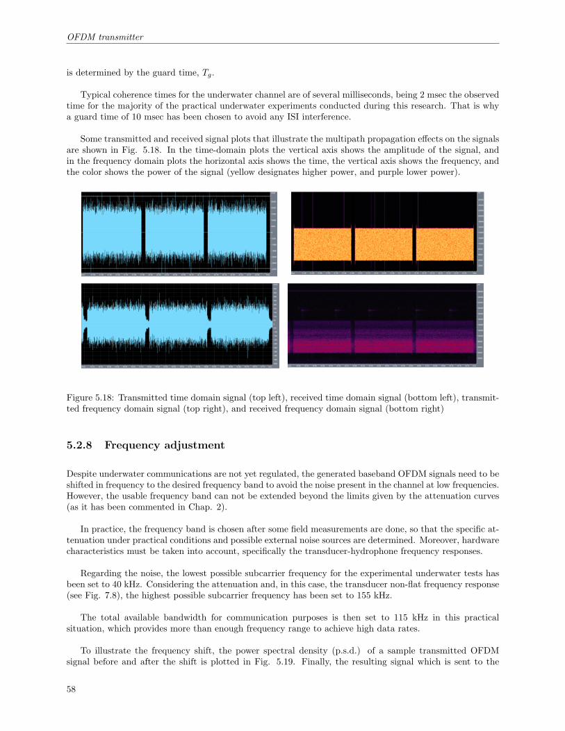
OFDM transmitter
is determined by the guard time, Tg.
Typical coherence times for the underwater channel are of several milliseconds, being 2 msec the observedtime for the majority of the practical underwater experiments conducted during this research. That is whya guard time of 10 msec has been chosen to avoid any ISI interference.
Some transmitted and received signal plots that illustrate the multipath propagation effects on the signalsare shown in Fig. 5.18. In the time-domain plots the vertical axis shows the amplitude of the signal, andin the frequency domain plots the horizontal axis shows the time, the vertical axis shows the frequency, andthe color shows the power of the signal (yellow designates higher power, and purple lower power).
Figure 5.18: Transmitted time domain signal (top left), received time domain signal (bottom left), transmit-ted frequency domain signal (top right), and received frequency domain signal (bottom right)
5.2.8 Frequency adjustment
Despite underwater communications are not yet regulated, the generated baseband OFDM signals need to beshifted in frequency to the desired frequency band to avoid the noise present in the channel at low frequencies.However, the usable frequency band can not be extended beyond the limits given by the attenuation curves(as it has been commented in Chap. 2).
In practice, the frequency band is chosen after some field measurements are done, so that the specific at-tenuation under practical conditions and possible external noise sources are determined. Moreover, hardwarecharacteristics must be taken into account, specifically the transducer-hydrophone frequency responses.
Regarding the noise, the lowest possible subcarrier frequency for the experimental underwater tests hasbeen set to 40 kHz. Considering the attenuation and, in this case, the transducer non-flat frequency response(see Fig. 7.8), the highest possible subcarrier frequency has been set to 155 kHz.
The total available bandwidth for communication purposes is then set to 115 kHz in this practicalsituation, which provides more than enough frequency range to achieve high data rates.
To illustrate the frequency shift, the power spectral density (p.s.d.) of a sample transmitted OFDMsignal before and after the shift is plotted in Fig. 5.19. Finally, the resulting signal which is sent to the
58

OFDM transmitter
transmitter circuitry is shown in Fig. 5.20.
Figure 5.19: OFDM signal p.s.d. (K=16384, 8-PSK, B=115kHz) before frequency adjustment (left) andafter (right)
Figure 5.20: Sample transmitted OFDM signal with K=16384, 8-PSK, and B=115kHz. Synchronizationpreamble and OFDM blocks
59


Chapter 6
OFDM receiver
The OFDM system receiver is designed according to the characteristics of the underwater channel. Thefrequency selectivity, the non-uniform Doppler Effect, and the time-varying multipath in the consideredchannel is taken into account to choose the most appropriate techniques.
The implemented system is introduced and the most important parts are explained in depth. In addition,the methods to quantify the performance of the system are commented.
6.1 Receiver design
The OFDM system receiver has been designed according to the transmitter model commented in Sec. 5.1,and its block diagram is the one shown in Fig. 6.1.
Figure 6.1: Receiver scheme
Once the receiving side hardware receives the OFDM signal from the channel, some band-pass FIRfiltering is applied to it in order to assure a successful synchronization and minimize the out band noise.After the filtering is performed, a time synchronization algorithm provides an accurate reference for thereception of the OFDM blocks.
It must be noted that the synchronization is performed before converting the signal to baseband, although
61

OFDM receiver
it could be done after the signal is shifted to baseband without a change in the achieved results.
It is at that point that the OFDM blocks are downshifted in frequency, and the FFT demodulationcalculates the complex raw constellation points.
The detector performs the post-FFT algorithm to retrieve the constellation points by cancelling thechannel effects. In it, the deinterleaving, parallel-to-serial conversion and FEC decoding are included, sothat the output is directly a sequence of detected scrambled bits. All the mentioned blocks are includedinside the detector to decrease the implementation complexity, as the coherent detector algorithm performsa coding-oriented detection to better estimate the channel (see Sec. 6.5.2).
Finally, the descrambler assesses the detected bits (which in the case of the video files are passed to theMPEG-4 decoder to display the detected video).
6.2 FIR filtering
The selected band-pass filter is designed according to the signal useful bandwidth and it aims to removethe out-of-band noise so that the signal looks clean before applying the synchronization technique. Despitethe signal did not present much interference in the experimental readings, it is highly recommendable toinclude this kind of filter, as other transmissions or external noise sources could affect the signal shape dueto out-of-band components.
The type of filter and the key parameters are shown in Tab. 6.1. The parameter WN is used to representthe edges of the pass band (as in the filter used to clip and filter in Sec. 5.2.6), as
WN = [flow, fhigh], where flow =F0 − 0.055B
Fs, and fhigh =
FK−1 + 0.055BFs
(6.1)
where B represents the useful bandwidth of the OFDM signal, F0 and FK−1 represent the first and lastsubcarrier frequencies, Fs is the sampling frequency, and the calculated edges, WN , are digital frequenciesin the range [0...1/2].
Filter type FIROrder 128
Gain at WN (dB) -6
Table 6.1: Filter parameters
To illustrate the effects of the implemented filtering, the power spectral densities (p.s.d) of the receivedsignal and the transfer function of the filter is shown in Fig. 6.2, and a sample received signal before andafter filtering can be seen in Fig. 6.3.
6.3 Time synchronization
The synchronization algorithm that has been included in the OFDM system receiver consists of a cross-correlation computation between the received signal after the FIR filtering application and the synchroniza-tion preamble (which is known at the receiver end).
62

OFDM receiver
Figure 6.2: Power spectral density (p.s.d.) of the received signal and the FIR filter response (B=115 kHz).The vertical axis indicates the signal power related to the maximum power in dB
Figure 6.3: Received signal before filtering (top), and after filtering (bottom) with B=115 kHz, 8-PSK,K=16384
63

OFDM receiver
Due to the properties of the selected preamble (see Sec. 5.2.7), the result of the cross-correlation algorithmshows a high peak where the preamble is detected in the received signal, with high probability (if no in-bandand high distorting noise is present).
The cross-correlation is computed for a length of Nsynch+Npause, where Nsynch is the number of samplesof the synchronization preamble, and Npause is the number of samples between the preamble and the firstOFDM block. The implementation selects the start of the received portion of signal to synchronize bychecking the amplitude of the signal. When the signal reaches a 70% of its highest value, it is assumed thatin this part the synchronization preamble is received.
The results of the synchronization algorithm for a sample received signal in a 200 meters underwater linkare shown in Fig. 6.4.
Figure 6.4: Synchronization preamble followed by a pause (top), received signal after filtering used as theinput of the synchronization algorithm (center), and cross-correlation between preamble and signal (bottom).OFDM parameters: B=115 kHz, 8-PSK, K=16384
6.4 FFT demodulation
The FFT algorithm is used to retrieve the subcarriers’ received symbols before channel treatment, by usingthe complementary method to the IFFT modulator. The applied equation is
y(k) =Ns−1∑l=0
sr(l)e−j2πkl/Ns , k = 0, ..., Ns − 1 (6.2)
where Ns is the number of samples during a symbol time, and sr(l) is the received sampled signal. An
64
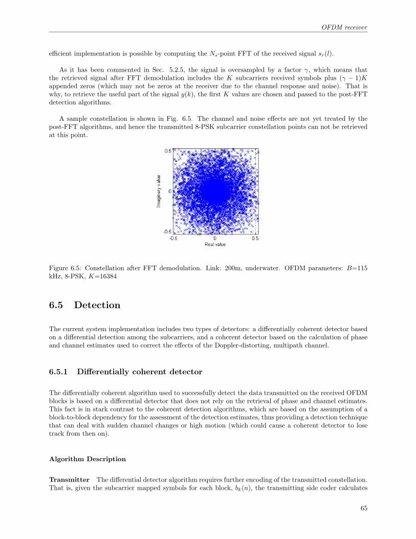
OFDM receiver
efficient implementation is possible by computing the Ns-point FFT of the received signal sr(l).
As it has been commented in Sec. 5.2.5, the signal is oversampled by a factor γ, which means thatthe retrieved signal after FFT demodulation includes the K subcarriers received symbols plus (γ − 1)Kappended zeros (which may not be zeros at the receiver due to the channel response and noise). That iswhy, to retrieve the useful part of the signal y(k), the first K values are chosen and passed to the post-FFTdetection algorithms.
A sample constellation is shown in Fig. 6.5. The channel and noise effects are not yet treated by thepost-FFT algorithms, and hence the transmitted 8-PSK subcarrier constellation points can not be retrievedat this point.
Figure 6.5: Constellation after FFT demodulation. Link: 200m, underwater. OFDM parameters: B=115kHz, 8-PSK, K=16384
6.5 Detection
The current system implementation includes two types of detectors: a differentially coherent detector basedon a differential detection among the subcarriers, and a coherent detector based on the calculation of phaseand channel estimates used to correct the effects of the Doppler-distorting, multipath channel.
6.5.1 Differentially coherent detector
The differentially coherent algorithm used to successfully detect the data transmitted on the received OFDMblocks is based on a differential detector that does not rely on the retrieval of phase and channel estimates.This fact is in stark contrast to the coherent detection algorithms, which are based on the assumption of ablock-to-block dependency for the assessment of the detection estimates, thus providing a detection techniquethat can deal with sudden channel changes or high motion (which could cause a coherent detector to losetrack from then on).
Algorithm Description
Transmitter The differential detector algorithm requires further encoding of the transmitted constellation.That is, given the subcarrier mapped symbols for each block, bk(n), the transmitting side coder calculates
65

OFDM receiver
the differentially encoded symbols that must be transmitted for each subcarrier, dk(n), as
dk(n) = dk−1(n)bk(n), k = 0, ...,K − 1 (6.3)
where the first subcarrier symbol is initialized as d−1(n) = 1. Note that the input QPSK symbols,bk(n), need to be on + constellation to assure that only 4 possible complex points are the output of thedifferential coder (also in + constellation). Thus, a 45◦ shift is required from the mapped constellation.Sample differential encoded constellations are shown in Fig. 6.6.
Figure 6.6: Differential encoded QPSK constellation (left) and 8-PSK constellation (right)
After the differential coding is performed, the dk(n) symbols are passed to the IFFT modulator (Sec.5.2.5).
Receiver The receiver gets the subcarriers’ complex points in the OFDM blocks contained in the receivedsignal, once the FFT demodulation is performed. The received values, yk(n), can be decomposed as
yk(n) = Hk(n)dk(n)ejθk(n) (6.4)
where Hk(n) represents the channel effect (a complex value for each block n and subcarrier k, containingthe amplitude attenuation and the phase shift), and θk(n) represents the phase shift due to the motion-induced Doppler effect.
As it can be easily retrieved from the previous equation, taking into account the assumption that thechannel estimates, Hk(n), and the phase estimates, θk(n), are similar between adjacent subcarriers, themapped symbols, bk(n), can be extracted by applying the following equation:
yk(n)yk−1(n)
=Hk(n)dk(n)ejθk(n)
Hk−1(n)dk−1(n)ejθk−1(n)≈ dk(n)dk−1(n)
= bk(n) (6.5)
In the case that multiple receivers are used, an average between the points obtained with all of them isperformed. A sample detected constellation is shown in Fig. 6.7, before and after the decision is made.
A couple of last comments must be made about the differential detector, regarding (1) the data rate ofa differential detection transmission and (2) the possible input constellations.
66

OFDM receiver
Figure 6.7: Detected constellation (left) and decided values (right) with differential detection. OFDMparameters: B=115 kHz, 8-PSK, K=16384
Regarding (1), the fact that there is one subcarrier in each OFDM block used to initialize the algorithmdirectly implies that there is one subcarrier unused in the OFDM transmission. In the practical implemen-tation, there is no reduction in data rate for the implemented system as a pilot is relocated on that firstsubcarrier to avoid the loss in data rate.
Finally, with reference to (2), the differential detector can only be used with PSK constellations, as theapplied algorithm does not take into account amplitude differences, and the encoding scheme is not designedto deal with QAM constellations (the differentially encoded symbols would result in a sequence of complexpoints with gradually increasing amplitude).
6.5.2 Coherent detector
The coherent algorithm used to perform the detection of the received OFDM blocks is the Low ComplexityOFDM Detector for Underwater Acoustic Channels [15]. It is an adaptive algorithm for OFDM signaldetection on Doppler-distorted, time-varying multipath channels. It focuses on a low complexity post-FFTsignal processing using adaptive channel estimation over the blocks. Non-uniform Doppler compensationacross subbands is performed using a single adaptively estimated parameter representing the Doppler ratefor each block.
Algorithm Description
After the application of the FFT algorithm, the received symbol values for each subcarrier k in the blockn, yk(n), are stored as a column vector that contains the complex points for each receiving element. Oncethese values are assessed, the algorithm performs the following steps (experimental underwater detectionexamples are provided in the referenced figures):
1. Assessment of a first data estimate dk1(n) using MMSE combining of the different receivers for eachsubcarrier k in the block n. To do so, it uses the phase offset θk(n − 1) and the channel frequency-domain coefficient Hk(n − 1) calculated in the previous block, along with a normalization parameterγk(n− 1) according to the amplitude of the channel coefficient (see Fig. 6.8).
dk1(n) = γk(n− 1)H′k(n− 1)yk(n)e−jθk(n−1) (6.6)
67

OFDM receiver
Figure 6.8: Constellation after FFT (left), and dk1 estimates (right) for an OFDM signal with K=16384,B=115 kHz, and 8-PSK subcarrier modulation
2. Calculation of an angular offset ∆θk(n) between the assessed dk1(n), and either the pilot symbols thatwere transmitted in the block, or a second estimate that corrects the block-to-block motion by usingthe Doppler coefficient from the last block. The performed steps are:
(a) (if no pilots are included) Retrieval of the estimate dk2(n), given by the following equation:
dk2(n) = γk(n− 1)H′k(n− 1)yk(n)e−jθk(n) = dk1(n)e−ja(n−1)ωkT′
(6.7)
(b) Calculation of the reference for the angular offset measurement, dk(n). Considering that dk(n)are the transmitted symbols, and K(n) is the pool of pilot subcarriers, it is given by
dk(n) ={
dk(n) if k ∈ K(n)decision[dk2(n)] otherwise
(6.8)
(c) Finally, the angular offset is assessed by evaluating the following scalar product:
∆θk(n) = 〈dk1(n)d∗k(n)〉 (6.9)
3. Assessment of the Doppler coefficient a(n) (Fig. 6.9) from the angular offsets ∆θk(n) by calculatingthe mean over the considered channels (being K the total number of subcarriers).
a(n) =1K
K−1∑k=0
∆θk(n)ωkT ′
(6.10)
Alternatively, the implementation can use only the pilot channels for phase tracking purposes, so thatthe dk2(n) estimate do not have to be computed, and the previous mean, a(n), is performed over thepilot subcarriers.
4. Calculation of the phase offset θk(n) (Fig. 6.10) for each subcarrier using the Doppler coefficient a(n).
θk(n) = θk(n− 1) + a(n)ωkT ′ (6.11)
5. Retrieval of a second more accurate data estimate, dk(n), using MMSE combining of the differentreceivers for each subcarrier k in the block. This estimate includes the correction of the possible tiltof the constellation due to the motion-induced Doppler distortion (see Fig. 6.11).
dk(n) = γk(n− 1)H′k(n− 1)yk(n)e−jθk(n) = dk1(n)e−ja(n)ωkT′
(6.12)
68

OFDM receiver
Figure 6.9: a estimates for an OFDM signal with K=16384, B=115 kHz, and 8-PSK subcarrier modulation
Figure 6.10: θk estimates in radians for an OFDM signal with K=16384, B=115 kHz, and 8-PSK subcarriermodulation. The plot includes the estimates for k=0, k=8191 and k=16383
Figure 6.11: dk1 estimates (left) and phase corrected dk estimates (right) for an OFDM signal with K=16384,B=115 kHz, and 8-PSK subcarrier modulation
69

OFDM receiver
6. Coding-oriented detection. The symbols are detected in blocks of multiple codewords so that the databits can be directly retrieved and some errors corrected (see Fig. 6.12).
dk(n) ={
dk(n) if k ∈ K(n)decision[dk(n)] otherwise
(6.13)
Figure 6.12: Phase-corrected dk estimates (left) and symbol decisions (right) for an OFDM signal withK=16384, B=115 kHz, and 8-PSK subcarrier modulation
7. Calculation of the channel estimates Hk(n) as explained in the next section.
8. Assessment of the normalization parameters γk(n) from the received values yk(n), the assessed phaseoffsets θk(n), and the second set of data estimates dk(n). A high SNR regime is supposed, so the noisevariance σ2
z is omitted.
γk(n) =(σ2z + H′k(n)Hk(n)
)−1
≈(H′k(n)Hk(n)
)−1
(6.14)
The algorithm is initialized using Hk(1) = yk(1)d∗k(1), a(1) = 0 and θk(1) = 0. For a correct performance,the receiver must know the transmitted symbols dk(1) to accurately initialize the channel estimates, so atraining sequence is transmitted in the first OFDM block.
Channel Estimation Algorithm
A low-complexity channel estimation algorithm known as Sparse Channel Estimation [16] is used in the timedomain. Sparsing of the channel impulse response leads to an improved performance, reducing the errorvariance. In this case, instead of implementing the complete algorithm, which includes the selection of thenumber of samples L ≤ K of the impulse response of the channel, the full-sized impulse response is used bychoosing L = K.
The channel estimates to be used in the next block must be calculated after the assessment of the detectedsymbols using the coherent detector algorithm. To do so, the channel estimation technique performs thefollowing steps (experimental underwater channel examples are shown in the referenced figures):
1. Calculation of the first frequency-domain channel estimates from the received values yk(n), the phaseoffsets θk(n) and the set of data decisions and pilots dk(n) (see Fig. 6.13).
70

OFDM receiver
Xk(n) = yk(n)e−jθk(n)d∗k(n), k = 0, ...,K − 1 (6.15)
Figure 6.13: Channel frequency-domain estimates Xk for an OFDM signal with K=16384, B=115 kHz, and8-PSK subcarrier modulation
2. Application of the IFFT algorithm to get the first time-domain channel estimates xl(n) from Xk(n)(see Fig. 6.14).
xl(n) =1K
K−1∑k=0
Xk(n)e+j2πkl/K , l = 0, ...,K − 1 (6.16)
3. Application of the sparsing by simply truncating the time-domain channel coefficients (see Fig. 6.14).A threshold αc is defined so that every time-domain channel coefficient below this value is set to zero.After the truncation is performed, the new time-domain channel response xl(n) is taken.
Figure 6.14: Channel time-domain estimates xl (left) and truncated coefficients xl (right) for an OFDMsignal with K=16384, B=115 kHz, and 8-PSK subcarrier modulation
4. Adaptive channel estimation to calculate the time-domain channel estimates applying the followingalgorithm (see Fig. 6.15):
hl(n+ 1) = λhl(n) + (1− λ)xl(n) (6.17)
71

OFDM receiver
5. Application of the FFT algorithm to get the final frequency-domain channel estimates used in the nextblock (see Fig. 6.15):
Hk(n) =K−1∑l=0
hl(n)e−j2πkl/K , k = 0, ...,K − 1 (6.18)
Figure 6.15: Channel updated time-domain estimates hl (left) and final frequency-domain estimates Hk
(right) for an OFDM signal with K=16384, B=115 kHz, and 8-PSK subcarrier modulation
6.6 Performance analysis
The performance of the system is quantified by using the concepts of (1) Mean Square Error (MSE) of theretrieved constellation points, and (2) Bit and Symbol Error Rates (BER and SER).
6.6.1 MSE
Regarding the MSE, it indicates the distance from the detected symbols (before a decision is made) to thetransmitted complex points in the constellation (see Fig. 6.16). Two types of MSE are evaluated, onethat indicates the performance depending on the frequency subcarriers (MSE-frequency), and another thatindicates the performance over the transmitted OFDM blocks (MSE-time).
The MSE-time calculation is evaluated over the K subcarriers, for each OFDM block, as
MSEt(n) =1K
K−1∑k=0
|dk(n)− dk(n)|2 (6.19)
And the MSE-frequency gives the mean square error over N received OFDM blocks, as
MSEf (k) =1N
N∑n=1
|dk(n)− dk(n)|2 (6.20)
72

OFDM receiver
Figure 6.16: MSE concept. Detected symbols before decision, dk (grey stars), and transmitted symbols, dk(blue circles)
The system performance can be then evaluated over time, while the subcarriers’ performance can also bestudied (normally those subcarriers that are received with more energy will have lower MSE). Sample MSEplots are shown in Fig. 6.17 and Fig. 6.18 for the underwater channel. Excellent performance is achievedwhen the MSE is below -5 dB, while otherwise the results can vary depending on the FEC coding.
Figure 6.17: MSE-time in dB (8-PSK subcarrier modulation, K=16384, BCH(63,18), B=115 kHz)
6.6.2 Bit and Symbol Error Rates
The Bit Error Rate (BER) is calculated as the total number of wrong bits divided by the amount oftransmitted bits. It is assessed for both the coded sequence (before the FEC decoding is performed) and thedecoded sequence of bits. This last result gives a direct indication of whether the transmitted sequence iscorrectly retrieved or not.
Sample BER plots are shown in Fig. 6.19. The coded BER is higher than the decoded BER, as it maybe expected.
The Symbol Error Rate (SER) is calculated as the total number of wrong symbols (before the coding-oriented decision is performed) divided by the total amount of symbols in the transmission. It is both assessedover the frequency subcarriers and the OFDM blocks, so as to give an indication of the error performancealong the transmission time, as well as for the different subcarriers.
73

OFDM receiver
Figure 6.18: MSE-frequency in dB (8-PSK subcarrier modulation, K=16384, BCH(63,18), B=115 kHz)
Figure 6.19: Coded sequence BER (left) and decoded sequence BER (right). The black solid line representsthe mean BER. OFDM parameters: 8-PSK subcarrier modulation, K=16384, BCH(63,18), B=115 kHz
74
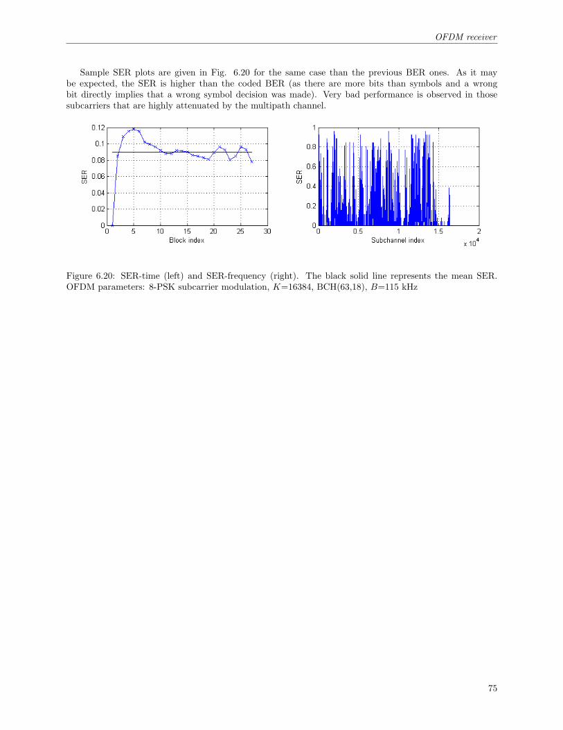
OFDM receiver
Sample SER plots are given in Fig. 6.20 for the same case than the previous BER ones. As it maybe expected, the SER is higher than the coded BER (as there are more bits than symbols and a wrongbit directly implies that a wrong symbol decision was made). Very bad performance is observed in thosesubcarriers that are highly attenuated by the multipath channel.
Figure 6.20: SER-time (left) and SER-frequency (right). The black solid line represents the mean SER.OFDM parameters: 8-PSK subcarrier modulation, K=16384, BCH(63,18), B=115 kHz
75

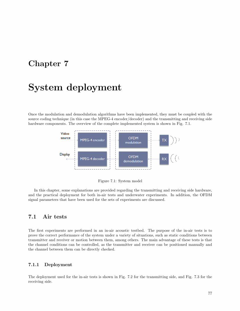
Chapter 7
System deployment
Once the modulation and demodulation algorithms have been implemented, they must be coupled with thesource coding technique (in this case the MPEG-4 encoder/decoder) and the transmitting and receiving sidehardware components. The overview of the complete implemented system is shown in Fig. 7.1.
Figure 7.1: System model
In this chapter, some explanations are provided regarding the transmitting and receiving side hardware,and the practical deployment for both in-air tests and underwater experiments. In addition, the OFDMsignal parameters that have been used for the sets of experiments are discussed.
7.1 Air tests
The first experiments are performed in an in-air acoustic testbed. The purpose of the in-air tests is toprove the correct performance of the system under a variety of situations, such as static conditions betweentransmitter and receiver or motion between them, among others. The main advantage of these tests is thatthe channel conditions can be controlled, as the transmitter and receiver can be positioned manually andthe channel between them can be directly checked.
7.1.1 Deployment
The deployment used for the in-air tests is shown in Fig. 7.2 for the transmitting side, and Fig. 7.3 for thereceiving side.
77

System deployment
Figure 7.2: Air tests transmission block diagram
Figure 7.3: Air tests reception block diagram
The wavefiles that contain the OFDM signals are generated using the developed MATLAB application(user’s manual provided in Annex A) at the transmitting side laptop, and then the GNU Radio interface(a set of tools for the creation of Software Defined Radios, SDR, which uses the Universal Software RadioPeripheral, USRP, as an interface with the transmitting and receiving hardware) is used to send the signalto the laptop speaker.
On the receiving side, the signal is acquired by a number of microphones (one in the case of only onereceiving element, or more if spatial diversity is used), and the laptop soundcard acts as an interface withthe MATLAB application, which records the signal and demodulates it.
7.1.2 Hardware
The hardware components that have been used for the implementation are described in this section. Theyare:
• Laptop/GNURadio: The transmitting side laptop is used to generate the wavefiles with MATLAB andthen, once the signals are stored, the GNU Radio platform is used to send the wavefiles to the USRPboard. This last step involves the use of a Python script to transmit the files to the USRP and fromit to the transmitting hardware, which in this case is a laptop speaker.
• USRP LFTX: The Universal Software Radio Peripheral (USRP) board is used as an interface thatallows the transmission of the generated acoustic signals by using a high sampling rate (in this project1 Mbps is used) of the analog wavefile provided by the laptop computer. More information about theUSRP board can be found in [24].
• Speaker: The speaker that is used for the tests is a normal laptop speaker connected to the USRPtransmitter connector.
78
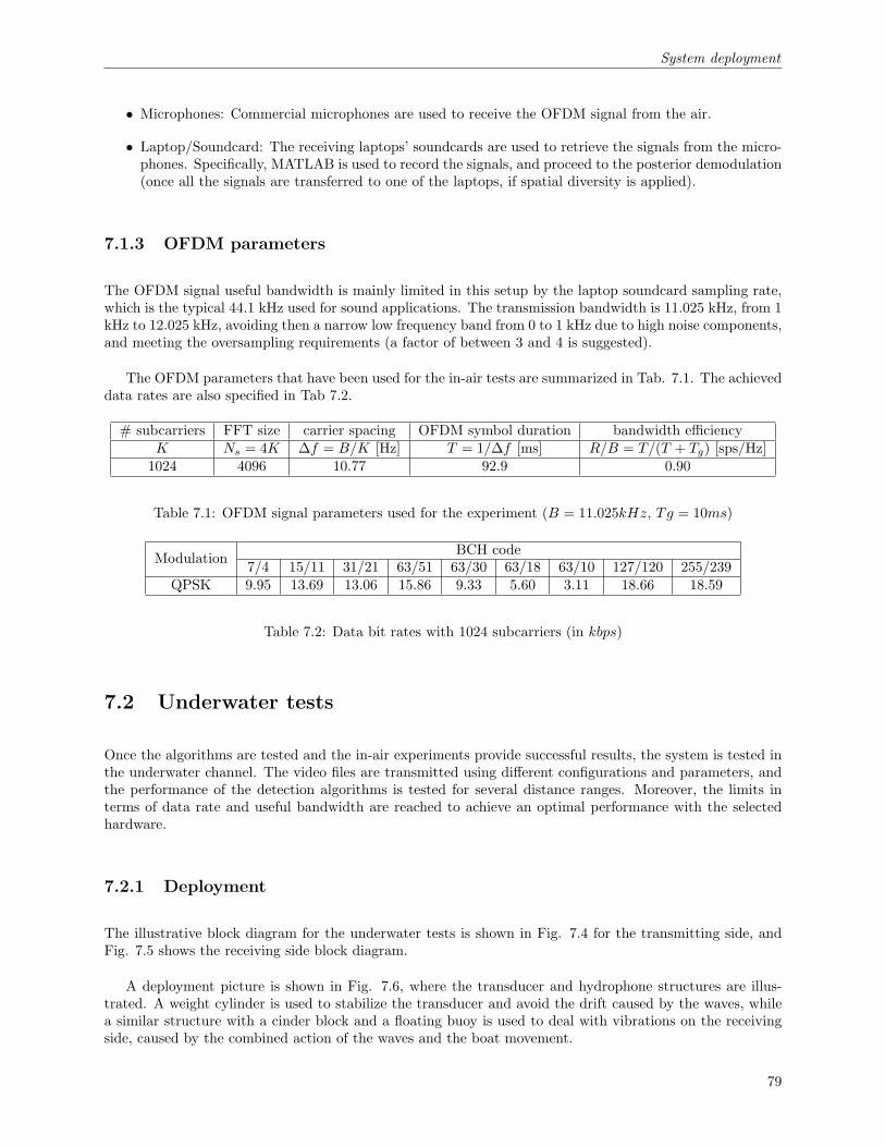
System deployment
• Microphones: Commercial microphones are used to receive the OFDM signal from the air.
• Laptop/Soundcard: The receiving laptops’ soundcards are used to retrieve the signals from the micro-phones. Specifically, MATLAB is used to record the signals, and proceed to the posterior demodulation(once all the signals are transferred to one of the laptops, if spatial diversity is applied).
7.1.3 OFDM parameters
The OFDM signal useful bandwidth is mainly limited in this setup by the laptop soundcard sampling rate,which is the typical 44.1 kHz used for sound applications. The transmission bandwidth is 11.025 kHz, from 1kHz to 12.025 kHz, avoiding then a narrow low frequency band from 0 to 1 kHz due to high noise components,and meeting the oversampling requirements (a factor of between 3 and 4 is suggested).
The OFDM parameters that have been used for the in-air tests are summarized in Tab. 7.1. The achieveddata rates are also specified in Tab 7.2.
# subcarriers FFT size carrier spacing OFDM symbol duration bandwidth efficiencyK Ns = 4K ∆f = B/K [Hz] T = 1/∆f [ms] R/B = T/(T + Tg) [sps/Hz]
1024 4096 10.77 92.9 0.90
Table 7.1: OFDM signal parameters used for the experiment (B = 11.025kHz, Tg = 10ms)
Modulation BCH code7/4 15/11 31/21 63/51 63/30 63/18 63/10 127/120 255/239
QPSK 9.95 13.69 13.06 15.86 9.33 5.60 3.11 18.66 18.59
Table 7.2: Data bit rates with 1024 subcarriers (in kbps)
7.2 Underwater tests
Once the algorithms are tested and the in-air experiments provide successful results, the system is tested inthe underwater channel. The video files are transmitted using different configurations and parameters, andthe performance of the detection algorithms is tested for several distance ranges. Moreover, the limits interms of data rate and useful bandwidth are reached to achieve an optimal performance with the selectedhardware.
7.2.1 Deployment
The illustrative block diagram for the underwater tests is shown in Fig. 7.4 for the transmitting side, andFig. 7.5 shows the receiving side block diagram.
A deployment picture is shown in Fig. 7.6, where the transducer and hydrophone structures are illus-trated. A weight cylinder is used to stabilize the transducer and avoid the drift caused by the waves, whilea similar structure with a cinder block and a floating buoy is used to deal with vibrations on the receivingside, caused by the combined action of the waves and the boat movement.
79

System deployment
Figure 7.4: Underwater tests transmission block diagram
Figure 7.5: Underwater tests reception block diagram
80

System deployment
Figure 7.6: Underwater tests deployment
7.2.2 Hardware
The hardware components that have been used for the underwater implementation are:
• Laptop/GNURadio: Exactly as in the in-air tests, the transmitting side laptop is used to generate thewavefiles with MATLAB (the application manual is provided in Annex A) and then, once the signalsare stored, the GNU Radio platform is used to send the wavefiles to the USRP board. A Python scriptis used to transmit the files to the USRP and from it to the transmitting hardware, which in this caseis the PA50 APEX power amplifier coupled with the transducer by an impedance matching circuit.On the receiving side, the laptop receives the wavefile from the USRP via another GNU Radio Pythonscript, and the demodulation is performed.
• USRP LFTX: As in the in-air case, the USRP board is used as an interface that allows the transmissionof the generated acoustic signals by sampling at 1 Mbps the analog wavefile provided by the laptopcomputer. More information about the USRP board can be found in [24].
• PA50 APEX power amplifier: The signal transmitted by the USRP board is further amplified bythe PA50 APEX power amplifier, to adjust the signal power to the transmission requirements in theunderwater channel. The power response of the PA50 APEX power amplifier is shown in 7.7. Forfrequencies lower than 200 kHz, the output voltage is maximized.
• Impedance matching circuitry: Prior to sending the signal to the transducer, an impedance matchingcircuit adjusts the signal for maximum power transmission to the transducer. It involves the use ofcapacitors, inductors and transformers.
• ITC-1042 transducer: The selected transducer is an omnidirectional ITC-1042, which is a broadbandpiezoelectric device whose main advantage is the high output power compared to other commerciallyavailable models. Its directivity pattern and Transmitting Voltage Response (TVR) are shown in Fig.7.8. As it can be observed in the TVR plot, the response has a resonance frequency, and it decays atlower and higher frequencies, thus limiting the transmission bandwidth (mainly at the high frequencyend, which is not observed in the plot).
• Reson TC4032 hydrophone: The Reson TC4032 ultra-wideband omnidirectional hydrophone has beenchosen for the reception of the acoustic OFDM signal. Its most important characteristic is the high
81
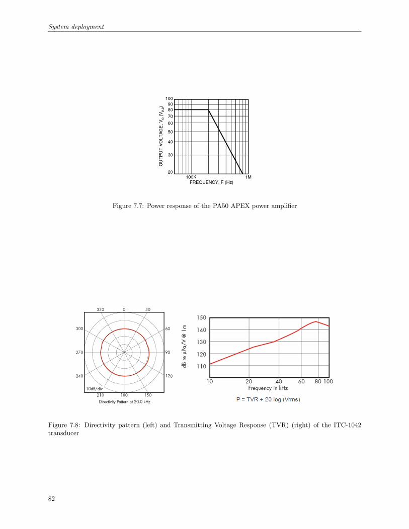
System deployment
Figure 7.7: Power response of the PA50 APEX power amplifier
Figure 7.8: Directivity pattern (left) and Transmitting Voltage Response (TVR) (right) of the ITC-1042transducer
82

System deployment
sensitivity at a wide range of frequencies (it can typically operate in the 10-150 kHz range), whichmakes it appropriate for the transmission of low-power signals or its use in high attenuated channels.The horizontal directivity pattern and receiving sensitivity is provided in Fig. 7.9.
Figure 7.9: Horizontal directivity pattern (left) and receiving sensitivity (right) of the Reson TC4032 hy-drophone
• Reson VP2000 preamplifier: Once the signal is picked by the hydrophone, the Reson VP2000 pream-plifier receives it, and filtering is performed. The characteristics of the high-pass and low-pass filtersare given in Fig. 7.10. As it can be seen, the filter response is adjustable depending on the signalfrequency components.
Figure 7.10: High-pass filter (left) and low-pass filter (right) frequency responses of the Reson VP2000preamplifier
• USRP LFRX: In the underwater setup, the USRP board is also used on the reception side. Again, itacts as an interface that allows the reception of the acoustic signal by sampling at 1 Mbps the analogwavefile provided by the Reson VP2000 preamplifier, and transmitting it to the receiving side laptopcomputer.
7.2.3 OFDM parameters
The underwater experiments fully utilize the USRP high sampling rate capabilities, both on the transmissionside and the reception side. As a result of that, the frequency allocation is not limited by the maximum
83

System deployment
sampling rate, which in this implementation is as high as 1 Mbps. Thus, the signal is allocated from40 kHz to 155 kHz (with a useful bandwidth of 115 kHz), taking into account both the low frequencynoise characteristics, and high attenuation at high frequencies, along with the transducer-hydrophone pairfrequency responses (as it was commented in Sec. 5.2.8).
Regarding the number of subcarriers, K=16384 is the ideal case for the undertaken transmissions, as ahigher data rate is achieved. In spite of that, the case K=8192 has also been used in several situations dueto:
1. The separation between subcarriers, ∆f , is larger, and, as a consequence, the frequency synchronizationis not as critical (the Inter-Carrier Interference, ICI, is not as pronounced).
2. The symbol time is smaller, and hence the assumption that the channel estimates and the phaseestimates do not differ much from one block to the next is more accurate.
The OFDM parameters that have been used for the underwater tests are summarized in Tab. 7.3. Theachieved data rates are also specified in Tab 7.4. The two different values for the number of subcarriers aretaken into consideration, and the modulation types that provide a best performance are also specified.
# subcarriers FFT size carrier spacing OFDM symbol duration bandwidth efficiencyK Ns = 5K ∆f = B/K [Hz] T = 1/∆f [ms] R/B = T/(T + Tg) [sps/Hz]
8192 40960 14.04 71.2 0.8816384 81920 7.02 142.5 0.93
Table 7.3: OFDM signal parameters used for the experiment (B = 115kHz, Tg = 10ms)
K Modulation BCH code7/4 15/11 31/21 63/51 63/30 63/18 63/10 127/120 255/239
8192QPSK 100.84 138.66 132.36 160.72 94.54 56.73 31.51 189.08 188.298-PSK 151.27 207.99 198.54 241.08 141.81 85.09 47.27 283.62 282.44
16-QAM 201.69 277.32 264.71 321.44 189.08 113.45 63.03 378.16 376.59
16384QPSK 107.46 147.75 141.04 171.26 100.74 60.45 33.58 201.48 200.648-PSK 161.19 221.63 211.56 256.89 151.11 90.67 50.37 302.22 300.97
16-QAM 214.92 295.51 282.08 342.52 201.48 120.89 67.16 402.97 401.29
Table 7.4: Data bit rates with 8192 and 16384 subcarriers (in kbps)
84

Chapter 8
Experimental results
After the system is implemented and all the hardware components are selected, the experimental part of thework begins. Three types of experiments are designed to prove the correctness of the selected algorithmsand test the system performance under a variety of situations.
First, some simulations are designed to provide the first results and check the system performance. Afterthat, some in-air testing is done to further check the overall implementation with a simple channel. Finally,underwater tests are performed and a thorough analysis is provided.
The different types of tests are explained in this chapter, and multiple results support the performanceexplanations.
8.1 Simulation tests
The first experiments are performed in a simulated channel, so that the wavefiles are generated with theWAV Generator application (see Annex A) and the wavefile input to the detector is created with the channelsimulator application (see Sec. A.1.4). The objectives of the tests are: (1) checking the performance resultswith different subcarrier modulations (both the signal generation and detection), and (2) checking the systemperformance for different simulated distances.
8.1.1 Description
The channel simulator includes 3 steps: the simulation of the multipath channel, the simulation of thedistance attenuation in an underwater channel, and the underwater noise addition. The block diagram isshown in Fig. 8.1.
As it can be seen in the simulator block diagram, the multipath channel (block 1) is simulated by addingthe generated OFDM signal, shifted in time and scaled by a given reflection coefficient, to itself. In theundertaken simulations, 3 arrivals have been considered (at 0 msec (direct path), 1 msec, and 2 msec), withdifferent reflection coefficients (1, 0.6 and 0.3, respectively).
The signal attenuation is then applied to the resulting wavefile (block 2 in the block diagram). The A(l, fc)coefficient, where l is the transmission distance and fc is the center frequency of the useful bandwidth, is
85

Experimental results
Figure 8.1: Simulator. Block diagram
calculated using the equation 2.1. The frequency-dependent attenuation through the useful bandwidth hasbeen simplified, and a coefficient is calculated for all the subcarriers.
Finally, a real underwater noise file is added (block 3 in the block diagram) to simulate the backgroundnoise in the underwater channel. The noise file is a sample from previous underwater noise-recording exper-iments done in the Gulf of Mexico during the first months of 2009.
It must be taken into account the fact that no time variation is considered in the simulator implemen-tation. One of the most important characteristics (and more difficult to detect than other ones) of theunderwater channel, and any communication channels indeed, is its variation through time. As a result, theachieved performance for the simulated transmissions is much better than the one for the real underwaterchannel.
With reference to the OFDM parameters, the K=16384 subcarriers case from the underwater testingconfiguration has been taken into account (see Sec. 7.2.3).
8.1.2 Subcarrier modulations
Five types of constellations have been tested with the channel simulator (QPSK, 8-PSK, 16-QAM, 32-QAMand 64-QAM). The selected distance is 400 m, and the detected constellations are plotted in Fig. 8.2 andFig. 8.3.
Furthermore, a Mean Square Error (MSE) and bit error rate (BER) study has been done for the differenttransmissions, with the aim to quantize the detection performance for the different subcarrier modulationtypes. The results are shown in Fig. 8.4 and Fig. 8.5.
8.1.3 Distances
The next set of simulated transmissions regards the detection performance for a transmitted 8-PSK constel-lation at different distances between transmitter and receiver. The selected distances have been 200 m, 400m, and 600 m. The constellation plots are shown in Fig. 8.6, while the MSE and BER are shown in Fig. 8.7and Fig. 8.8. For the BER plot, only the non-zero curves are shown.
86
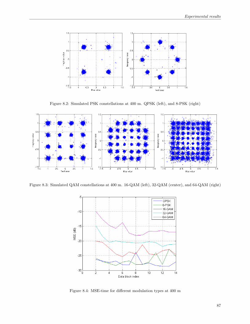
Experimental results
Figure 8.2: Simulated PSK constellations at 400 m. QPSK (left), and 8-PSK (right)
Figure 8.3: Simulated QAM constellations at 400 m. 16-QAM (left), 32-QAM (center), and 64-QAM (right)
Figure 8.4: MSE-time for different modulation types at 400 m
87
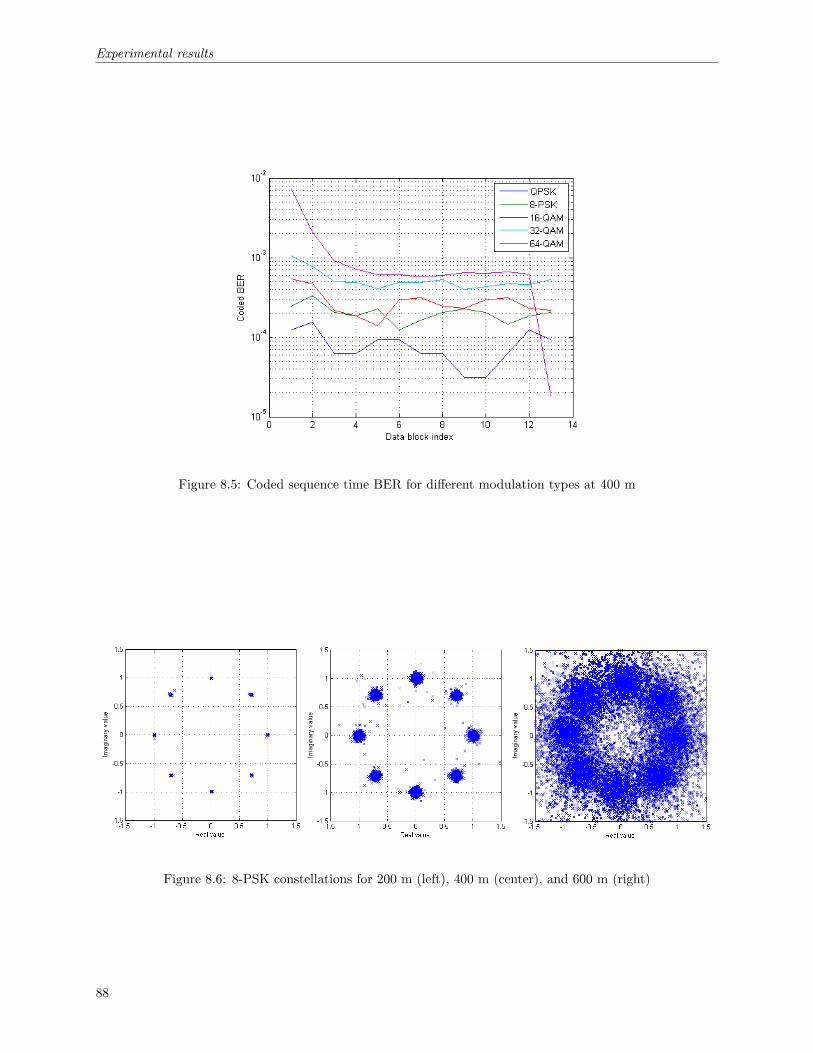
Experimental results
Figure 8.5: Coded sequence time BER for different modulation types at 400 m
Figure 8.6: 8-PSK constellations for 200 m (left), 400 m (center), and 600 m (right)
88

Experimental results
Figure 8.7: MSE-time for different distances
Figure 8.8: Time BER for different distances
89

Experimental results
8.2 Air tests
There is basically one reason why the in-air tests have been considered, which is the fact that the channelbetween transmitter and receiver is entirely known. Indeed, the indoor testbed provides an easy way ofchecking the detection performance under several channel conditions, which can be recreated by moving thetransmitter (speaker) and/or receiver (microphone).
Specifically, there have been 3 approaches for the in-air tests: a multipath analysis, a motion effectsstudy, and a performance check for multiple receivers.
8.2.1 Multipath
The first thing that has been studied is the correspondence between the real channel and the time domainchannel estimates that are observed with the coherent detector. The channel estimates and the speaker-microphone layout are shown in Fig. 8.9.
Figure 8.9: Chanel time-domain estimates (left) and experiment layout (right)
The real channel possible reflections are the ceiling and wall reflections of the laboratory. After somecalculations, the correspondence is established between these reflections and the multipath arrivals seen inthe channel estimates. The details are shown in Tab. 8.1.
Arrival time (msec) Path distance (m) Correspondence2.18 0.74 Wall reflection5.71 1.94 Ceiling reflection
Table 8.1: Multipath study
The following must be noted regarding the multipath absorption: as the speed of sound underwater isapproximately five times the speed of sound in air, the multipath that is absorbed in a given time periodfor the underwater channel is for a five times longer path than the absorbed multipath in air. As a result,the conditions of the system underwater are much better, in terms of guard time design (a five times shorterguard time will be needed to absorbe the same reflected paths).
90

Experimental results
8.2.2 Motion
The second set of tests aim at checking the motion track for different types of relative speed and accelerationbetween transmitter and receiver. Two sets of experiments have been designed, one with moderated motionand another with fast motion, and different behaviors have been found for the different detector types.
Moderated motion
The moderated motion case involves the movement of the receiver (microphone) with uniform speed towardsthe transmitter (speaker), followed by a gradual decrease of velocity until a stop, and then another movementwith uniform speed in the opposite direction, moving away from the speaker. The experiment layout andthe phase estimates are shown in Fig. 8.10.
Figure 8.10: Phase estimates in radians for k=0, k=511 and k=1023 (left) and experiment layout (right),with moderated motion and coherent detection
In the phase estimates plot, the increase in the phase estimates value corresponds to the approach ofthe microphone towards the speaker, while the decrease in the phase estimates value corresponds to thesubsequent separation between them. The relative speed between transmitter and receiver is approximately10 cm/s (1 meter movement for a 10-second transmission), and the phase tracking algorithm is, in this case,perfectly acquiring the motion-induced Doppler effect.
Finally, the BER results for both the coded and decoded sequence are shown in Fig. 8.11. As it maybe expected, in the figure some increases are seen in the parts where the acceleration, or phase gradient, ishigh. The decoded BER is lower than the coded one, as the decoder can correct an important number ofrandom errors.
Fast motion
The fast motion case involves a first static period of time, followed by a quick left-right motion of themicrophone (which involves both high speed and acceleration), and another static period at the end. Thephase estimates and experiment layout in this case is shown in Fig. 8.12. The detection results with thecoherent detector are shown in Fig. 8.13.
As it can be seen, the decoded sequence BER for the coherent detector is null for the static period, and
91

Experimental results
Figure 8.11: Coded sequence time BER (left) and decoded sequence time BER (right), with moderatedmotion and coherent detection
Figure 8.12: Phase estimates in radians for k=0, k=511 and k=1023 (left) and experiment layout (right),with fast motion and coherent detection
Figure 8.13: Decoded sequence time BER, with fast motion and coherent detection
92

Experimental results
then it increases to 0.5, where it remains until the end of the transmission. In this case the selected detectorloses track of the channel estimates, as the motion is too high for the slow block-to-block change assumption.
An interesting change in performance is seen when the fast motion is followed by a static period withthe microphone exactly put in the same location than in the beginning of the experiment. For this case, thedetector can still track the channel after the motion finishes, as the adaptive algorithm has a memory of theprevious channel state.
To solve the tracking problem for fast varying channels (in the first case, in which the location is changed),the differentially coherent detector is used. For the same kind of motion, the detection results with differentialdetection are shown in Fig. 8.14.
Figure 8.14: Decoded sequence time BER (left) and experiment layout (right), with fast motion and differ-ential detection
As it may be expected, some BER peaks are seen when the highest acceleration is applied to the micro-phone, but after these the detector can easily get on track again, as it does not rely on the estimates for pastblocks. The differential detector is then appropriate for fast motion conditions, while in static or moderatedmotion environments the coherent detection achieves better results.
A final comment must be made regarding the motion correspondence between the in-air transmissions andunderwater environments. As it has been pointed out before, the speed of sound underwater is approximatelyfive times the speed of sound in air, so that the relative speed that can be tolerated in an underwaterimplementation is five times the applied motion in-air. That is, along with the multipath absorption,another advantage of the underwater channel.
8.2.3 Multiple receivers
The last set of in-air experiments aim to demonstrate the performance improvement with the use of multiplereceiving elements. In the practical implementation, another microphone is used to receive the same OFDMsignal, and an MMSE combining of the signal is performed in the detector.
Two sets of results are evaluated. The first is for static conditions (Fig. 8.15), where an improvementof around 50% in the coded BER is observed. The second set of results (Fig. 8.16) corresponds to thefast motion case, and a BER reduction for the multiple receiving elements case is also observed even withextreme detection conditions (the high BER peaks are due to the high acceleration). The MSE curves arealso lower when spatial diversity is used, representing a more accurate retrieval of the constellation.
93
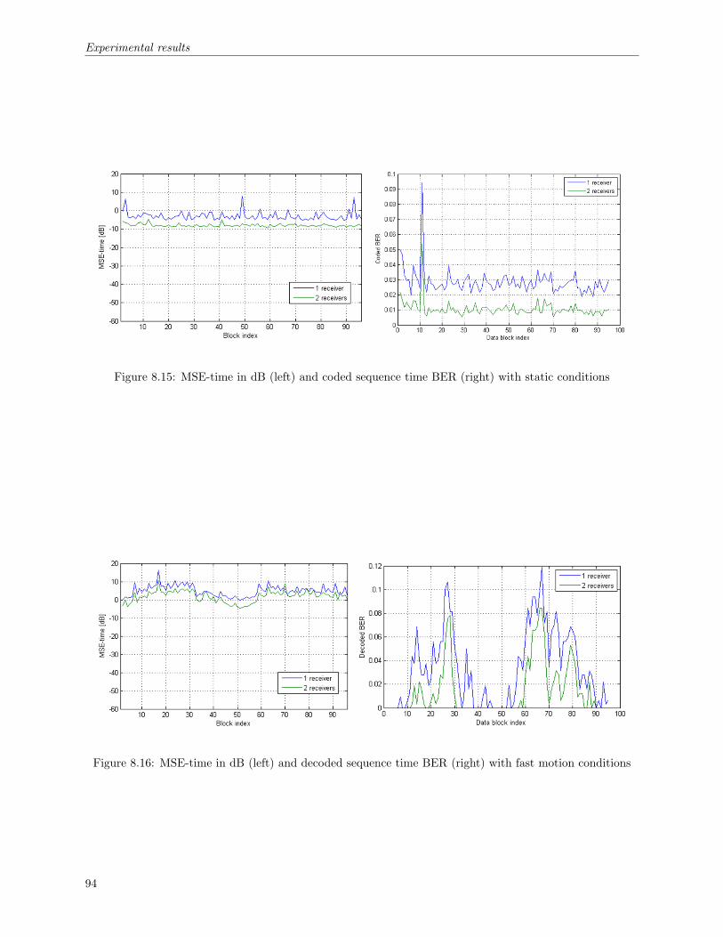
Experimental results
Figure 8.15: MSE-time in dB (left) and coded sequence time BER (right) with static conditions
Figure 8.16: MSE-time in dB (left) and decoded sequence time BER (right) with fast motion conditions
94

Experimental results
8.3 Underwater tests
The underwater experiments have been conducted at the MIT Sailing Pavilion, and four main types of testingare designed, depending on the parameter of study. They are: FEC coding tests, subcarrier modulationsanalysis, distance experiments, and consistency tests. Before the detection performance is evaluated, somevideo detection considerations are discussed.
8.3.1 Video detection
Prior to the practical performance quantification, a targeted overall BER must be established in order to havea reference for the selection of the different parameters. That is why numerous video sequences are evaluatedwith different detected BER, from the first sets of preparatory experiments (with different configurationsand parameters). A summary of the results is shown in Fig. 8.17.
Figure 8.17: Sample image detection. BER=0% (left), BER=0.12% (center), and BER=1.17% (right)
The conclusion after the analysis is that the detected video BER must be below 0.1% in order to have aqualitatively acceptable detection. Due to that, a target BER of 10−3 is selected.
Before proceeding to the next experiments, it must be said that in the implemented system the FECcoding does not protect differently the headers and the video data in the MPEG-4 video stream, so thata low number of errors in the frame headers can cause the corruption of an entire image. In subsequentdevelopments, stronger FEC coding could be applied to frame headers and other important side information,while the lighter coding could be used for the video data. By doing this, higher decoded BER could beacceptable.
8.3.2 FEC coding
A data sequence of 16 OFDM blocks is transmitted in a 200 meters link with different BCH codings, andthe performance in terms of decoded BER is assessed. The evaluated results are shown in Fig. 8.18.
As it can be observed, the only curve that is consistently located close to the horizontal axis is the one forthe BCH(63,30) code. Moreover, the curves for the BCH(63,18) and BCH(63,10) codes can not be seen as thedecoded BER for these cases is always zero. Therefore, a coding ratio of 2.10 (the one for the BCH(63,30))is the minimum for a consistent performance.
Some explanation must be made about the decoded BER increase for the rest of the cases. As thecoherent detector has been used to evaluate the different coding types, there are error propagation effects
95
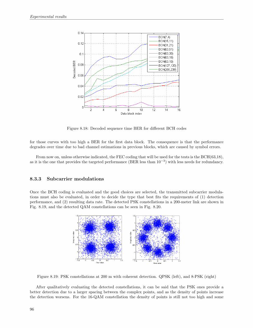
Experimental results
Figure 8.18: Decoded sequence time BER for different BCH codes
for those curves with too high a BER for the first data block. The consequence is that the performancedegrades over time due to bad channel estimations in previous blocks, which are caused by symbol errors.
From now on, unless otherwise indicated, the FEC coding that will be used for the tests is the BCH(63,18),as it is the one that provides the targeted performance (BER less than 10−3) with less needs for redundancy.
8.3.3 Subcarrier modulations
Once the BCH coding is evaluated and the good choices are selected, the transmitted subcarrier modula-tions must also be evaluated, in order to decide the type that best fits the requirements of (1) detectionperformance, and (2) resulting data rate. The detected PSK constellations in a 200-meter link are shown inFig. 8.19, and the detected QAM constellations can be seen in Fig. 8.20.
Figure 8.19: PSK constellations at 200 m with coherent detection. QPSK (left), and 8-PSK (right)
After qualitatively evaluating the detected constellations, it can be said that the PSK ones provide abetter detection due to a larger spacing between the complex points, and as the density of points increasethe detection worsens. For the 16-QAM constellation the density of points is still not too high and some
96
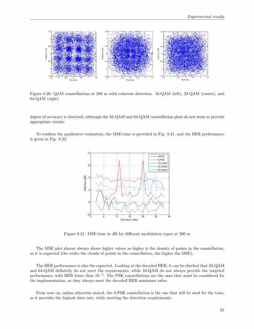
Experimental results
Figure 8.20: QAM constellations at 200 m with coherent detection. 16-QAM (left), 32-QAM (center), and64-QAM (right)
degree of accuracy is observed, although the 32-QAM and 64-QAM constellation plots do not seem to provideappropriate results.
To confirm the qualitative evaluation, the MSE-time is provided in Fig. 8.21, and the BER performanceis given in Fig. 8.22.
Figure 8.21: MSE-time in dB for different modulation types at 200 m
The MSE plot almost always shows higher values as higher is the density of points in the constellation,as it is expected (the wider the clouds of points in the constellation, the higher the MSE).
The BER performance is also the expected. Looking at the decoded BER, it can be checked that 32-QAMand 64-QAM definitely do not meet the requirements, while 16-QAM do not always provide the targetedperformance, with BER lower than 10−3. The PSK constellations are the ones that must be considered forthe implementation, as they always meet the decoded BER minimum value.
From now on, unless otherwise stated, the 8-PSK constellation is the one that will be used for the tests,as it provides the highest data rate, while meeting the detection requirements.
97

Experimental results
Figure 8.22: Coded sequence time BER (left) and decoded sequence time BER (right) for different modulationtypes at 200 m
8.3.4 Distances
The distance tests aim at defining the maximum distance range at which the system achieves the targetedperformance. The development of these tests is possible after measuring the transmitter-receiver distanceon the receiving side, which is located in a boat, with a GPS device. The main parameters to study are thepower and overall performance of the system, and the channel differences.
To illustrate the power conditions at different distances, the Signal to Noise (SNR) ratio vs. subcarrierfrequency is plotted for the different distances in Fig. 8.23. As it may be expected, the SNR decreases ashigher is the distance. The underwater channel attenuation combined with the transducer frequency responseaffect the received signal, and due to that the higher frequencies are more attenuated than the lower ones.
Figure 8.23: Average SNR in dB vs. frequency for different transmitter-receiver distances
98

Experimental results
To evaluate the overall performance, the MSE plot is shown in Fig. 8.24 for the attempted cases. Theperformance is close to the expected, as for higher distances the MSE is usually higher.
Figure 8.24: MSE-time in dB for different transmitter-receiver distances
In addition, the BER for different distances is evaluated and given in Fig. 8.25.
The trends are also the expected, with outstanding detection results for the 200-meter link, for whichthe decoded BER is zero. For the other cases, the BER is generally above 10−3, so 200 meters is selected asthe maximum distance with the available hardware and practical channel conditions.
A comment about the channel conditions must be made for the 400-meter and 1-kilometer link. For thesecases, a high degree of variation has been noticed from one run of tests to the next, due to the differentlocation of the hydrophone (the location is approximately the same, but as the receiver is in a boat a differentplace may be chosen on different days).
8.3.5 Consistency
To finish the underwater experiments, a consistency study is done for the 200-meter link between transmitterand receiver. The 8-PSK constellation is chosen, and two types of BCH coding are used for the comparison:the BCH(63,18) and the BCH(63,30). A number of consecutive video transmissions of several seconds (2.61seconds for the lighter code and 4.14 seconds for the heavier code) are attempted, with a one-second differencebetween each other.
The consistency results are evaluated in terms of MSE and BER. The MSE plot is shown in Fig. 8.26,and the BER plot is provided in Fig. 8.27.
There is a correlation between the crossing of the two BCH types’ lines in the MSE plot and the crossingof the coded BER curves, as the MSE provides an estimation of the detector performance. The decodedBER is always well below the targeted 10−3 for the BCH(63,18), while the BCH(63,30) is normally abovethis value.
The BCH(63,18) with 8-PSK in a 200 meters link can then be considered an appropriate choice, given
99
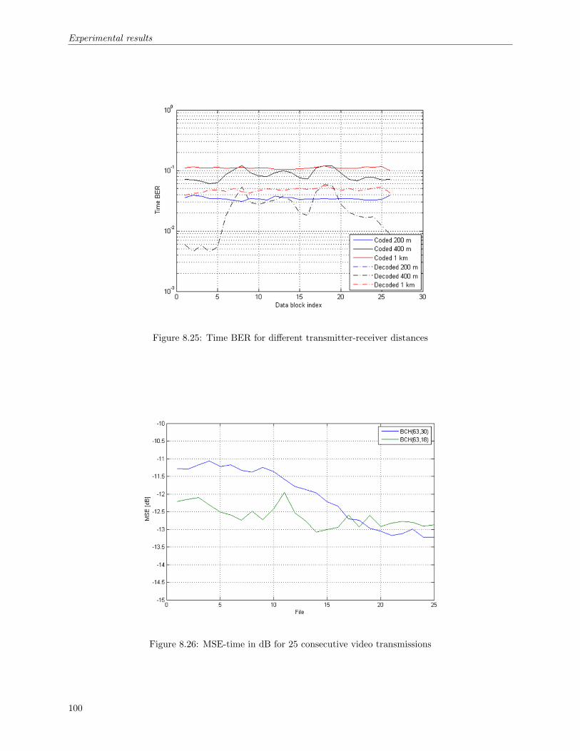
Experimental results
Figure 8.25: Time BER for different transmitter-receiver distances
Figure 8.26: MSE-time in dB for 25 consecutive video transmissions
100

Experimental results
Figure 8.27: Time BER for 25 consecutive video transmissions
the consistent performance through time.
The data rate performance is also appropriate for the transmission of video data, as 91 kbps is achievedwith the BCH(63,18). The frame rate for a real-time transmission is set to about 12 fps for a low qualityvideo (as it is commented in Sec. 3.3.2), providing a sufficient value to retrieve the motion of an underwatervideo, which is typically slow. If higher quality video is to be used, a decrease in the frame rate is required,as there is a compromise between frame rate and quality (this last dependent on resolution and MPEG-4compression ratio).
101


Chapter 9
Conclusions and future work
In the light of the results from the experiments, some conclusions may be given about the success of thecurrent research, according to the goals that were established for the project. These objectives were thetransmission of video data at appropriate data rates, with satisfactory detection performance in a certaindistance range.
Regarding the achieved data rates, the final OFDM system with the selected parameters exceeds theminimum 64 kbps bit rate for the transmission of the MPEG-4 low bit rate video. As a consequence of that,the goal is achieved.
With reference to the detection performance, the first video transmissions determined that a bit errorrate (BER) lower than 10−3 was necessary. The implemented system provides an even better BER than thisestablished upper bound, which illustrates the success while qualitatively evaluating the detected files.
Finally, the distance range has been limited to 200 meters for an excellent and consistent detection. Inspite of that, the performance of the system at higher distances may be better than the one suggested bythe results, as the system is sensitive to channel changes. As a wide range of results was achieved for the400-meter and 1-kilometer link, an appropriate selection of the location for the pair transducer-hydrophonemight provide excellent results at these distances, too.
It must be also noted that, in contrast with previous experiments done in the field, a high bandwidthis used for the video data transmissions. The useful bandwidth is dependent on the link distance (as it isstated in Sec. 2.2.3), thus allowing the use of high frequency ranges for short distance links (in this case themaximum attempted distance is 1 kilometer).
After these few conclusions about the work, some issues to be treated in the future must be explained.They can be classified into two groups: the practical implementation modifications, and the software changes.
About the practical issues, some underwater testing is required with multiple receiving elements, as atypical underwater system has no less than 4 receivers. Furthermore, multiple transmitting elements canalso be tested, in order to achieve either a higher data rate, or a better detection performance.
Further improvement can be achieved by stabilizing the transmitter-receiver setup, so that the bestlocations can be selected for the transducer and hydrophone. As it has been commented before, this couldmake a difference for the high distance cases.
Regarding the software implementation changes, online block processing must be considered in order to
103

Conclusions and future work
directly retrieve the video data in the field, with no need for recording wavefiles and processing them offline,on the dock or in the laboratory.
Finally, some research on video compression techniques is necessary in the case that higher quality istargeted, as higher compression ratios will become indispensable, and the MPEG-4 technique cannot providea much better compression performance than the one used in this work.
104

Bibliography
[1] M.Suzuki and T.Sasaki. Digital acoustic image transmission system for deep sea research submersible.Proc. IEEE Oceans’92 Conference, September 1992.
[2] L.Berkhovskikh and Y.Lysanov. Fundamentals of ocean acoustics. New York: Springer, 1982.
[3] R.Coates. Underwater acoustic systems. New York: Wiley, 1989.
[4] J.Proakis T.Wang and J.Zeidler. Techniques for suppression of intercarrier interference in OFDM sys-tems. Wireless Communications and Networking Conference, IEEE, vol.1, pp.39-44, March 2005.
[5] M.Stojanovic. On the relationship between capacity and distance in an underwater acoustic com-munication channel. Proc. First ACM International Workshop on Underwater Networks (WUWNet),September 2006.
[6] M.Stojanovic. Capacity of a relay acoustic channel. Proc. IEEE Oceans Conf., October 2007.
[7] H.Ando J.Kojima, T.Ura and K.Asakawa. High speed acoustic data link transmitting moving picturesfor autonomous underwater vehicles. Proc. International Symposium on Underwater Technology, April2002.
[8] M.Suzuki and T.Sasaki. Digital acoustic image transmission system for deep sea research submersible.Proc. IEEE Oceans’92 Conference, September 1992.
[9] V.Ingle D.Hoag and R.Gaudette. Low bit-rate coding of underwater video using wavelet-based com-pression algorithms. IEEE J. Oceanic Eng., vol. 22, pp. 393-400, April 1997.
[10] M.Stojanovic C.Pelekanakis and L.Freitag. High rate acoustic link for underwater video transmission.Proc. IEEE Oceans’03 Conference, September 2003.
[11] G.Lapierre J.Trubuil and J.Labat. Real time transmission of images and data through underwateracoustic channel: The Trident system. Proc. Geosciences and Remote Sensing Symposium, 2004.
[12] J.P.Beaujean. High-speed high-frequency acoustic modem for image transmission in very shallow waters.Proc. IEEE Oceans Conf., June 2007.
[13] Z.Weiquing et al. Signal processing for high speed underwater acoustic transmission of image (Marc2007). Proc. IEEE Oceans Conf., June 2007.
[14] J.Catipovic M.Stojanovic and J.Proakis. Phase coherent digital communications for underwater acousticchannels. IEEE Journal of Oceanic Engineering, vol.13, No.1, pp.100-111, January 1994.
[15] M.Stojanovic. Low complexity OFDM detector for underwater acoustic channels. IEEE Oceans Con-ference, September 2006.
[16] M.Stojanovic. OFDM for underwater acoustic communications: Adaptive synchronization and sparsechannel estimation. Proc. International Conference on Acoustics, Speech, and Signal Processing(ICASSP’08), April 2008.
105

BIBLIOGRAPHY
[17] M.Stojanovic L.Freitag B.Li, S.Zhou and P.Willet. Multicarrier underwater acoustic communicationsover fast-varying channels. IEEE Journal of Oceanic Engineering, April 2008.
[18] H.Wallace. Error detection and correction using the BCH code. 2001.
[19] X.Li and L.J.Cimini. Effects of clipping and filtering on the performance of OFDM. CommunicationsLetters, IEEE, vol. 2, no. 5, May 1998.
[20] A.Jayalath and C.Tellambura. Reducing the peak-to-average power ratio of orthogonal frequency divi-sion multiplexing signal through bit or symbol interleaving. Electronics Letters, vol. 36, no. 13, June2000.
[21] B.Krongold and D.Jones. A new tone reservation method for complex-baseband PAR reduction inOFDM systems. Acoustics, Speech and Signal Processing ICASSP’02, 2002.
[22] B.Krongold and D.Jones. An active-set approach for OFDM PAR reduction via tone reservation. SignalProcessing, IEEE Transactions, vol. 52, no. 2, February 2004.
[23] G.Rojo. Peak-to-average power ratio (PAR) reduction for acoustic OFDM systems. Proc. IEEEOceans’09 Conference, Biloxi, MS, October 2009.
[24] Firas Abbas Hamza. The USRP under 1.5X magnifying lens. GNU Radio project, June 2008.
106

Appendix A
User’s manual
The designed OFDM system is implemented in MATLAB and Graphical User Interfaces (GUI) are createdto facilitate the wavefile generation and demodulation process.
The different GUI that are included in the system are: the WAV Generator, which generates a wavefilefor transmission; the WAV Receiver, which receives and demodulates the OFDM signals from a single (for aone receiver system) or multiple (for more than one receiver system) wavefiles; and the WAV Plotter, whichplots signals from a transmitted or received wavefile.
Inside the main folder of the Acoustic Modem implementation, the GUI folder contains the different GUIthat are described in this section.
A.1 WAV Generator
The wavefile generator application aims at writing an OFDM signal to a wavefile to be transmitted to theselected channel. The GUI, input parameters, and output commands and files are explained in this section.
A.1.1 GUI
The designed GUI is shown in Fig. A.1. The different parameters must be selected in the checkboxes, pop-upmenus, and written in the editable boxes.
A.1.2 Parameters
The GUI input parameters are explained in Tab. A.1.
Apart from the GUI parameters, other parameters may be changed in the implementation scripts. Theseare:
• Frequency range parameters: the operating frequency band is defined in the script frequency params.m,which is located in the main folder of the Acoustic Modem system.
107

User’s manual
Figure A.1: WAV Generator GUI
Parameter Input type ExplanationCreate all the files Checkbox Create all the defined BCH codings’ files
Data from file Checkbox If checked, the data is taken from the chosen input file.If not checked, the data is taken from a random generator
Mix files Checkbox If checked, a mixed file containing the multiple BCH codings,separated in time, is created
Fast mix Checkbox If checked, a fast mixing process is performed.If not, a slow mixing for long signals is used
Differential detection Checkbox If checked, differential coding is used.If not, normal mapping is performed
Resynchronize Checkbox If checked, synchronization preambles are sent each 2 secondsEvaluate PAR Checkbox If checked, a PAR evaluation plot is shown
PAR Pop-up menu PAR technique to be appliedNumber of subcarriers Pop-up menu Number of subcarriers for the system, K
Modulation type Pop-up menu Subcarrier modulation typeBCH coding Pop-up menu BCH coding typeGuard time Editable box Guard time between OFDM blocks, in seconds
Total signal time Editable box Total signal time, if random data is used
Table A.1: WAV Generator input parameters
108

User’s manual
• Input data file: in the case that the data is from a file, the file that is used can be changed by runningthe file reader script. It is located in the data folder, and it is called get file data.m. The commandline information has the following format:
Possible input files:1) file_1...N) file_NChoose input file: nReading file...Done.Generating scrambling sequence...Done.Scrambling...Done.Saving data...Data saved.
where the possible input file names are shown from the files in the folder data/input files and theselection of one of them is followed by the scrambling of the file. The data is finally saved to be usedfor the transmission.
A.1.3 Output
The command line output has the following format:
TEST X*****Generating .wav*****Total transmission time: x.xx sec[1/6] Coding...
Done.[2/6] Mapping symbols in carriers...
Block 1...Done....Block N...Done.Done.
[3/6] Creating signal...Synch block 1...Modulating...
Block 1...Done....Block N...Done.
Done.Adding synch...Done.
[4/6] Writing to file...Done.
[5/6] Evaluation and plots...Skipped.
[6/6] Filtering...Done.
Done.
109

User’s manual
And the generated files are located in the folder sep tx, for the separated BCH coding files, and the foldersep rx, in the case that some mixing is done. A sample sep tx folder is shown in Fig. A.2.
Figure A.2: Sample sep tx directory after wavefile generation
The .wav file contains the OFDM signal wavefile, and two .mat files are created: one for the data analysis,and another one for the PAR analysis.
A.1.4 Channel simulator
The channel simulator script is located in the channel sim folder, and it is called channel simulator. Asample command line output after the execution of the script is:
Possible input files:1) filename_1.wav...F) filename_F.wavChoose OFDM signal file: fAdd noise (0/1): 1Possible input files:1) noise_1.wav...N) noise_N.wavChoose noise file: nAdd distance attenuation (0/1): 1Distance (km): d
The possible input files are taken from the sep tx folder, and are offered for selection. The noise filesmust be stored in the noise folder to be detected by the application, and finally a distance parameter isrequested for the attenuation.
The output wavefile is saved in the sep rx folder, under the same name than the one in the sep tx folder.A sample sep rx folder is shown in Fig. A.3.
A.2 WAV Receiver
The wavefile receiver application is designed to take the OFDM received signal from one or multiple files(depending on the number of receivers), demodulate and decode the data. The GUI, input parameters, andoutput commands and files are explained in this section.
110

User’s manual
Figure A.3: Sample sep rx directory after channel simulation
A.2.1 GUI
The designed GUI is shown in Fig. A.4. As in the generator GUI, the different parameters must be selectedin the checkboxes, pop-up menus, and written in the editable boxes.
A.2.2 Parameters
The GUI input parameters are explained in Tab. A.2.
Parameter Input type ExplanationReceive all the tests Checkbox Receive all the defined BCH codings’ files
Data from file Checkbox If checked, the data is saved in a file.If not checked, the data is not saved
PAR Pop-up menu PAR technique that has been appliedDifferential detection Checkbox If checked, differential coding is used.
If not, normal mapping is performedSeparate tests Checkbox If checked, the mixed file is taken and the BCH types are
separated. If not, the separated file is usedResynchronize Checkbox If checked, synchronization preambles are searched each
2 secondsInvert signals Checkbox If checked, the signal is multiplied by −1Make plots Checkbox If checked, the detection and analysis plots are shownSave results Checkbox If checked, the results and plots are saved in the results folder
Number of subcarriers Pop-up menu Number of subcarriers for the system, KModulation type Pop-up menu Subcarrier modulation type
BCH coding Pop-up menu BCH coding typeNumber of receivers Pop-up menu Number of receiving elements in the systemOutput file extension Pop-up menu File extension for the received file
Guard time Editable box Guard time between OFDM blocks, in secondsTotal signal time Editable box Total signal time, if random data is usedTime to analyze Editable box Time to be analyzed, if partial detection is aimed
Table A.2: WAV Receiver input parameters
Regarding the Invert signals checkbox, it has been included to deal with the inversion of the transmittedsignal by the USRP transmission Python script. Moreover, if partial detection is used and the specified timeis larger than the file total length, full detection is applied.
Apart from the GUI parameters, other parameters may be changed in the implementation scripts. Theseare:
111

User’s manual
Figure A.4: WAV Receiver GUI
112

User’s manual
• Frequency range parameters: as for the WAV Generator application, the operating frequency band isdefined in the script frequency params.m, which is located in the main folder of the Acoustic Modemsystem.
• Detector parameters: the detector parameters such as channel thresholds, update equations’ coefficientsor overlap-add coefficients can be modified in the file data type.m, which is also located in the mainfolder of the Acoustic Modem implementation.
A.2.3 Output
The command line output has the following format:
*****Receiving ./sep_rx/filename*****[1/3] Acquiring symbols...
Filtering receiver 1/Nr...Filtering done.Synchronizing receiver 1/Nr...Synchronization done.Demodulating receiver 1/Nr...Demodulation done....Filtering receiver Nr/Nr...Filtering done.Synchronizing receiver Nr/Nr...Synchronization done.Demodulating receiver Nr/Nr...Demodulation done.
[2/3] Post-FFT detecting (PAR_type=P, Differential=D)...Part 1/1...
Initializing...Done.Detecting block 1 of N...Done....Detecting block N of N...Done.
Post-FFT detection done.[3/3] Saving data...
Data saved.Rx done.
*****Analyzing data ./sep_rx/filename*****[1/2] Plotting detection results...
Detection results plotted.[2/2] Analyzing performance...
* Part 1/1:Decoded data length: Dl bytesCoded data length: Cl bytesBER after decoding: x.xxxxxxBER before decoding: x.xxxxxxAverage MSE: x.x dB
113

User’s manual
where the Nr receivers are filtered (the filtered wavefile is saved in the sep rx folder), synchronized anddemodulated. After the detection, an analysis is performed indicating data lengths in bytes, bit error rates(BER), and an average MSE.
The synchronization algorithm outputs the details as in Fig. A.5. Once the synchronization performanceis shown, the algorithm continues with the detection.
Figure A.5: Synchronization plot
The output plots are the ones shown in Fig. A.6 and Fig. A.7.
Finally, if the results are saved, they are located in the results folder as shown in Fig. A.8.
A.3 WAV Plotter
The wavefile plotter is an application that allows the user to generate the plots of the OFDM signals thatare transmitted and received. The file names must not be changed from the transmitted signal notation, sothat the application finds the wavefiles in the corresponding directories (sep tx and sep rx folders).
A.3.1 GUI
The designed GUI is shown in Fig. A.9. As in the previous GUI, the different parameters must be selectedin the checkboxes, pop-up menus, and written in the editable boxes.
114
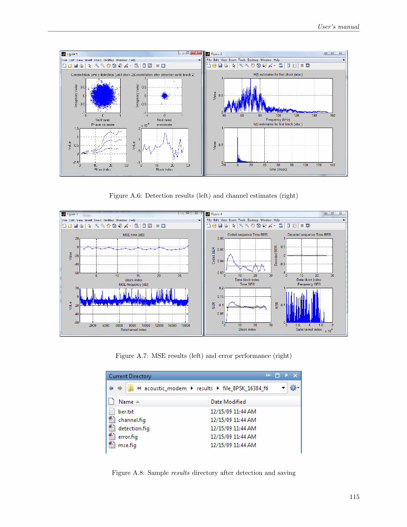
User’s manual
Figure A.6: Detection results (left) and channel estimates (right)
Figure A.7: MSE results (left) and error performance (right)
Figure A.8: Sample results directory after detection and saving
115

User’s manual
Figure A.9: WAV Plotter GUI
116

User’s manual
A.3.2 Parameters
The GUI input parameters are explained in Tab. A.3.
Parameter Input type ExplanationTransmitted signal Checkbox Plot a signal from the sep tx folder
Received signal Checkbox Plot a signal from the sep rx folderData from file Checkbox If checked, the data is from a file.
If not checked, the data is randomly generatedFile type Pop-up menu The type of file (single coding type or coding types mix)
Modulation type Pop-up menu Subcarrier modulation typeNumber of subcarriers Pop-up menu Number of subcarriers for the system, K
Code Pop-up menu BCH coding typeLength Editable box Length (samples or time) to be shown
Horizontal axis Pop-up menu Horizontal axis units (time -seconds-, or samples)
Table A.3: WAV Plotter input parameters
In the case that the length to be plotted is higher than the maximum length, a full signal plot is shown.
A.3.3 Output
The wavefile plotter outputs a plot with the selected files’ signals in the time or sample domain, as shownin Fig. A.10. In this example, a transmitted and received OFDM signal can be seen in the time domain.
117

User’s manual
Figure A.10: Plotted OFDM signals
118