Underwater visual census (UVC): Application and data

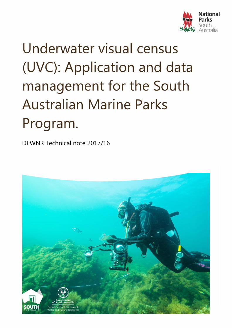
Underwater visual census

(UVC): Application and data

management for the South

Australian Marine Parks

Program. DEWNR Technical note 2017/16

Underwater visual census (UVC):

Application and data management for the

South Australian Marine Parks Program.

James Brook, David Miller, Shane Holland, Dimitri Colella and Danny Brock

Department of Environment, Water and Natural Resources

June, 2017

DEWNR Technical note 2017/16

DEWNR Technical note 2017/16 i


GPO Box 1047, Adelaide SA 5001

Telephone National (08) 8463 6946

International +61 8 8463 6946

Fax National (08) 8463 6999

International +61 8 8463 6999

Website www.environment.sa.gov.au

Disclaimer

The Department of Environment, Water and Natural Resources and its employees do not warrant or make any

representation regarding the use, or results of the use, of the information contained herein as regards to its

correctness, accuracy, reliability, currency or otherwise. The Department of Environment, Water and Natural

Resources and its employees expressly disclaims all liability or responsibility to any person using the information

or advice. Information contained in this document is correct at the time of writing.

This work is licensed under the Creative Commons Attribution 4.0 International License.

To view a copy of this license, visit http://creativecommons.org/licenses/by/4.0/.

© Crown in right of the State of South Australia, through the Department of Environment, Water and Natural

Resources 2017

ISBN 978-1-925668-12-4

Preferred way to cite this publication

Brook J, Miller D, Holland, S, Colella D and Brock D, 2017. Underwater visual census (UVC): Application and data

management for the South Australian Marine Parks Program. DEWNR Technical note 2017/16, Government of

South Australia, Department of Environment, Water and Natural Resources, Adelaide.

Download this document at http://www.marineparks.sa.gov.au/

http://www.environment.sa.gov.au/

http://creativecommons.org/licenses/by/4.0/

http://www.marineparks.sa.gov.au/

DEWNR Technical note 2017/16 ii

Foreword

The Department of Environment, Water and Natural Resources (DEWNR) is responsible for the management of the

State’s natural resources, ranging from policy leadership to on-ground delivery in consultation with government,

industry and communities.

High-quality science and effective monitoring provides the foundation for the successful management of our

environment and natural resources. This is achieved through undertaking appropriate research, investigations,

assessments, monitoring and evaluation.

DEWNR’s strong partnerships with educational and research institutions, industries, government agencies, Natural

Resources Management Boards and the community ensures that there is continual capacity building across the

sector, and that the best skills and expertise are used to inform decision making.

Sandy Pitcher

CHIEF EXECUTIVE

DEPARTMENT OF ENVIRONMENT, WATER AND NATURAL RESOURCES

DEWNR Technical note 2017/16 iii

Acknowledgements

Many people have participated in the collection of diver UVC data in South Australia (SA) over the years, far too

many to list individually (in particular those who have worked and helped out with the field program). However,

special mention needs to be made to those that have made consistent or large contributions to the SA reef

monitoring program. Our collaborative partners from University of Tasmania (UTas) have been instrumental to the

program from the beginning. These include Neville Barrett, Graham Edgar, Liz Oh, Rick Stuart-Smith and Toni

Cooper to name a few. In SA many people have also made significant contributions to this program. Bryan

McDonald initiated the program with UTas, while Ali Bloomfield, Yvette Eglinton, Ben Brayford, Alison Wright and

Simon Bryars have been regular divers and logistical coordinators.

We also thank Helen Owens, Mathew Royal and Mathew Miles (DEWNR) for their contributions to the

development of a system to input, store and output data within DEWNR’s corporate data storage system, and for

contributing to the documentation, classification and licencing processes for diver UVC data. Several of the

DEWNR staff mentioned above plus Colin Cichon are also thanked for their input at the various stages of editing

this report.

DEWNR Technical note 2017/16 iv

Contents

Foreword ii

Acknowledgements iii

Summary 1

1 Scope 2

2 UVC overview 3

2.1 Background 3

2.2 Overview of survey methods used in SA marine parks 3

2.2.1 Marine Protected Area (MPA) method 3

2.2.2 Reef Life Survey (RLS) method 3

3 Application of diver underwater visual census (UVC) methods 5

3.1 Approach prior to implementation (2004–14) 5

3.2 Approach post implementation (after 2014) 5

4 Data processing and management 9

4.1 Overview 9

4.2 Field preparation data 11

4.3 Data capture 11

4.4 Data processing and validation 11

4.4.1 Field validation 11

4.4.2 Data entry 12

4.4.3 Spreadsheet data validation 12

4.4.4 Photoquadrat image processing 13

4.4.5 Identification photo processing 14

4.5 Post processing data management and storage 14

4.5.1 Datasheets, data submission, checking and storage 14

4.5.2 DEWNR storage of dive survey data 15

4.6 Outputs and access 15

4.6.1 Data to support MER Program analysis and reporting 15

4.6.2 Spatial layers 15

4.6.3 Metadata 15

4.6.4 Archived photoquadrats, identification photos and scanned data sheets 16

4.7 Data classification and licencing 16

5 Appendices 18

A. Underwater Visual Census (UVC) survey locations prior to establishment of sanctuary zones in 2014

(using baseline MPA survey method) 18

B. Ongoing UVC monitoring sites (as of 2017) 24

C. Importing data from the University of Tasmania (UTas) national database 28

6 References 30

DEWNR Technical note 2017/16 v

List of figures

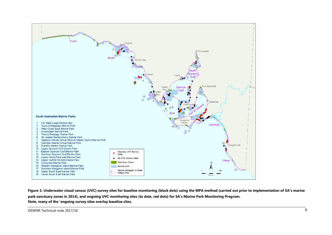
Figure 1: Underwater visual census (UVC) survey sites for baseline monitoring (black dots) using the MPA method

(carried out prior to implementation of SA’s marine park sanctuary zones in 2014), and ongoing UVC

monitoring sites (to date, red dots) for SA’s Marine Park Monitoring Program. 6

Figure 2. Dataflow, data classification and data licencing within DEWNR’s diver UVC monitoring program. 10

Figure 3. Import steps and ‘core’ data tables stored on DEWNR’s corporate network. 28

Figure 4. A detailed representation of the incoming data (from UTas) and the extraction process using the ’core’

database 29

List of tables

Table 1. Proposed bioregional monitoring program. 8

DEWNR Technical note 2017/16 1

Summary This report describes how the underwater visual census (UVC) by SCUBA divers is applied in the South Australia’s

Marine Parks Program to monitor subtidal reefs. It documents the process of UVC data capture, processing and

storage in a Department of Environment, Water and Natural Resources (DEWNR) corporate database.

Subtidal reefs were identified as a key ecological value of the South Australian Marine Parks Network. UVC is

currently one of the most common methods used to assess these ecosystems, and was recommended for use to

assess the effectiveness of the Marine Parks Network at protecting and conserving marine biodiversity.

Prior to Marine Park implementation a number of subtidal reefs across South Australia (SA) were surveyed using

the UVC Marine Protected Area (MPA) method developed by the University of Tasmania (UTas) to establish a

baseline. Since full implementation of marine parks in October 2014, a modified version of the Reef Life Survey

(RLS) UVC method (which was also developed by UTas) has been adopted to assess ecological change. The data

for both methods are largely compatible, with the RLS method having several advantages for ongoing monitoring,

one of which is the ability to recruit and train volunteer divers to collect data.

The ecological component of DEWNR’s Monitoring, Evaluation and Reporting (MER) Program focuses on priority

marine parks sanctuary zones (where most change due to marine park implementation is likely) in comparison to

suitable control sites outside the sanctuary zones. The monitoring design has taken a Before-After-Control-Impact

(BACI) or After Control-Impact (where no ‘Before’ data is available) approach. Diver UVC is used to compliment

other monitoring approaches (such as Baited Remote Underwater Video Systems (BRUVS) surveys), with some

sanctuary zones being sampled annually and others less frequently.

Sampling is conducted primarily during the warmer months between December to April when water temperatures

are higher and daylight hours are longer. As much as possible, individual sites are resurveyed at the same time of

year to reduce seasonal biases. Where possible, zones and sites are selected in such a way that broader spatial

patterns (e.g. spatial and physical gradients) can be considered in comparisons of multiple in-and-out sample sets.

A variety of data types are generated during the collection, processing and storage of UVC data. These include

field data, diver survey data (raw datasheets and electronic), reference and photoquadrat images, the final ‘point

of truth’ dataset, and the products derived from it (e.g. spatial layers, reporting outputs and documents). Standard

procedures and protocols are used in the collection and curation of this data at all stages of the process, to ensure

that data collection and processing is consistent across the Marine Parks Program now and into the future.

Data collected in SA is entered, processed and then sent to the UTas who hold the authoritative UVC national

dataset for the RLS and MPA Programs. DEWNR receives and stores extracted data for SA which is held in a

corporate database. Ultimately, data from this corporate storage point will be made available through DEWNR’s

‘Fauna Supertable’, Atlas of Living Australia, spatial layers, and internally through a purpose-built database in a

format suitable for analysis and other purposes (these products are under development).

Classification and licencing of UVC data and products is ‘Open’ by default in line with the Government of South

Australia’s Declaration of Open Data. Relevant datasets therefore are classified and licenced according to the

DEWNR classification guidelines to establish their confidentiality, integrity and availability. The bulk of the data

generated through the collection and processing stages leading to storage and production of outputs for the UVC

sampling program is considered ‘transitionary’ in nature, i.e. stages leading to the production of final, distributable

products, and as such, are considered as ‘not ready for public distribution’. This data is therefore classified ‘For

Official Use Only’ and archived.

To ensure transparency and provide guidance for individuals seeking knowledge about information collected

under the UVC Program, appropriate documentation and metadata records are produced for all relevant data. This

report and its appendices fulfill that role at the broadest level, forming a summary guide to the methodology, data

management and data storage. Metadata relating more directly to data collected in the field and subsequently

stored in the UTas and DEWNR corporate databases are available in the government’s Location SA system (LMS:

Dataset no. 2022).

https://data.environment.sa.gov.au/Content/Publications/DEWNR-TN-2017-20.pdf

http://digital.sa.gov.au/sites/default/files/content_files/declarations/Declaration-of-Open-Data.pdf

http://sdsidata.sa.gov.au/LMS/Reports/ReportMetadata.aspx?p_no=2022



1 Scope

Subtidal reefs were identified in Marine Park Baseline Reports (Bryars et al. 2016) as a key ecological value likely to

change with the implementation of marine parks. Underwater visual census (UVC) by divers is one of the main

ecological sampling methods currently being employed to monitor these systems and assess the long term

effectiveness of South Australia’s marine park network. The data collected by the UVC method will be used to

help answer key evaluation questions (KEQs): KEQ 1, KEQ 2 and KEQ 3 as identified in the South Australian Marine

Parks Monitoring, Evaluation and Reporting Plan (MER Plan, Bryars et al. 2017).

The aim of this report is to comprehensively describe the application of UVC to monitor subtidal reefs and

document UVC data capture, processing and storage in a DEWNR corporate database. This document will cover

the following areas:

underwater visual census methods

sampling approach and design

data entry and validation

data curation and storage

standard reporting outputs.

The purpose of the information provided is to:

demonstrate how ecological monitoring of subtidal reefs outlined in the SA Marine Parks MER Plan is

being implemented using UVC

ensure that standard procedures are followed during UVC surveys so that data collection and processing

is consistent across the Marine Parks Program now and into the future

facilitate access to the UVC data under the government’s ‘Open Data Policy’

provide a data platform upon which UVC ecological reporting outputs for the Marine Parks Performance

Program will be based.

It is anticipated that this will be a ‘live’ document such that any future changes to sampling methods, data capture

and technological advances can be incorporated as they arise.

https://data.environment.sa.gov.au/Coast-and-Marine/Coast-Marine-Management/Pages/home.aspx


2 UVC overview

2.1 Background

UVC by divers is the most widely used method for assessing subtidal reefs worldwide (Girolamo & Mazzoldi 2001,

Baron et al. 2004, Stuart-Smith et al. 2017), and in particular for assessing the effectiveness of marine reserves

(Barrett et al. 2007, Edgar et al. 2009, Soler et al. 2015). In a review of potential monitoring methods for the South

Australian Marine Parks Program, Bryars (2013) recommended the use of UVC in conjunction with BRUVS as

techniques for long term monitoring. Consequently, UVC has been adopted as one of the primary monitoring

methods to collect biological data that can be used to assess the long term effectiveness of the SA Marine Parks

Network.

Diver-based UVC surveys are ideal for marine protected areas as they are non-destructive and collect data across a

broad range of fish, invertebrate and macroalgal taxa, thus assessing the impact of protection at ecosystem,

habitat and individual species levels. Data is collected simultaneously from different trophic levels (e.g. primary

producers, grazers and predators) thus enabling the detection of change across different components of the

ecosystem. UVC is particularly effective for assessing species that are shy, reclusive or live in crevices in the reef

structure such as lobsters, abalone and cryptic fish (Holmes et. al. 2013).

2.2 Overview of survey methods used in SA marine parks

Various UVC methods are used around the world and in Australia. The most widespread and ongoing method

currently employed for temperate reef ecosystems is the Marine Protected Area (MPA) method and its derivative

the Reef Life Survey (RLS) method, both of which were developed by the University of Tasmania (UTas). The MPA

and RLS method are currently used for ecological monitoring of subtidal reefs in all Australian states.

2.2.1 Marine Protected Area (MPA) method

The UVC method used by UTas to monitor marine parks across southern Australia was first used at Maria Island in

Tasmania in 1992. This method, generally referred to as the ‘MPA method’ as it was developed for monitoring

marine protected areas (of which the SA marine parks are a subset), and is described in detail by UTas (2010; also

summarised in Edgar and Barrett 1999). These surveys were primarily undertaken by professional marine scientists.

In summary it uses three methods to survey three distinct components of reef communities:

Method 1: All fish and other large swimming animals, i.e. those that can be viewed while swimming in the

water column, above the macroalgal canopy or near the mouth of caves and ledges. The survey method is

a belt survey covering 200 m x 5 m on each side of a transect line.

Method 2: Mobile invertebrates and sedentary or cryptic fish, often hidden under ledges within caves, or

underneath the macroalgal canopy. The survey method is a belt survey covering 200 m x 1 m on one side

of a transect line.

Method 3: Macroalgae, including understorey species, sessile invertebrates and substrate information. The

survey method is a 0.25 m2 quadrat replicated 20 times at 10 m intervals along the transect line.

2.2.2 Reef Life Survey (RLS) method

The Reef Life Survey (RLS) Program was established in 2007 in order to make diver-based UVC surveys accessible

to well-trained community divers. RLS surveys were initially focused on temperate waters in Australia but have

grown into an international program. Most of the RLS data collected in South Australia has been in conjunction


with professional scientific divers at RLS training events, on dedicated RLS survey trips, by professional scientific

divers from government agencies or private consultancies.

The survey method was adapted from the MPA method and is described in detail by Reef Life Survey (2015). The

main differences to the MPA method are:

The macroalgae, sessile invertebrates and substrate component (Method 3) is surveyed using

photoquadrats rather than in-situ quadrat surveys.

The area covered by the invertebrate and cryptic fish survey (Method 2) is doubled by surveying on both

sides of the transect line (total area = 400 m2).

There is greater flexibility in the scalability and level of replication within surveys, with surveys based on a

number of independent 50 m transects rather than a single composite 200 m transect.


3 Application of diver underwater visual

census (UVC) methods

3.1 Approach prior to implementation (2004–14)

The University of Tasmania and their associated fisheries research faculty, (previously the Tasmanian Aquaculture

and Fisheries Institute, currently the Institute of Marine and Antarctic Studies; IMAS), commenced marine park

monitoring at Maria Island in Tasmania in 1992, before gradually extending to other temperate-water states

around Australia.

DEWNR undertook reef surveys in collaboration with UTas during a scientific expedition to the Althorpe Islands in

2004. Following this, DEWNR contracted UTas to undertake baseline UVC surveys of subtidal reefs in the

Encounter Region in 2004 as part of the establishment of the Encounter Pilot Marine Park (Edgar et al. 2006).

These surveys were conducted using the MPA method. This collaboration has continued between 2004 and 2014

via a series of Australian Research Council (ARC) research partnerships. The principle aim of the ARC research

partnerships was to collect as much baseline data as possible prior to full implementation of South Australia’s

marine parks network when fishing restrictions inside sanctuary zones (SZs) came into effect on 1 October 2014.

More than 150 sites were established during this period (Figure 1). Where possible the sites were located in areas

considered likely to become SZs in the future and thus form the basis of an ongoing long term monitoring

program.

The focus of the baseline surveys was to facilitate future detection of temporal change in protected zones. The

surveys were designed to minimise spatial variation that may confound the temporal signal. This was done by

assessing fixed sites through time, surveying along a fixed depth contour (generally 5 m or 10 m), and aggregating

data over a long distance (200 m) per site (Edgar et al. 2006). Sites were surveyed at the same time of year to

minimize seasonal effects (Edgar et al. 2006). Practical considerations for diving resulted in the choice of late

summer and autumn (when water temperatures are higher and daylight hours are longer) and a focus on 5 m sites

(allowing longer bottom time).

Following the finalisation of zoning in November 2012 it was apparent that some sites would become redundant

from the perspective of a marine parks Monitoring, Evaluation and Reporting (MER) Program using comparative

sites inside a SZ and sites outside but adjacent to a SZ (see maps in Section 4.1 of Bryars et al 2017). A summary of

the sites, locations and years resurveyed is shown in Appendix A.

3.2 Approach post implementation (after 2014)

Location of UVC monitoring

In October 2014 the Marine Park zoning became fully operational with fishing restrictions commencing inside the

83 SZs across the SA marine parks network. As outlined in the MER Plan (Bryars et al. 2017), SZs will be the main

focus of the ecological monitoring program in terms of detecting for change due to the management plans. With

current resourcing levels it is not feasible to undertake monitoring in all 83 SZs (nor is it necessary). To identify

where to allocate ecological monitoring effort a process was undertaken to prioritize the SZs based on their

ecological value, socio-economic importance and predicted changes (Bryars et al. 2017). As a consequence of this

process, 25 priority sanctuary zones were identified for monitoring (Bryars et al. 2017).

https://data.environment.sa.gov.au/Content/Publications/DEWNR-TR-2017-05.pdf


Figure 1: Underwater visual census (UVC) survey sites for baseline monitoring (black dots) using the MPA method (carried out prior to implementation of SA’s marine

park sanctuary zones in 2014), and ongoing UVC monitoring sites (to date, red dots) for SA’s Marine Park Monitoring Program.

Note, many of the ‘ongoing survey sites overlay baseline sites.


Monitoring rationale

The design of the ecological monitoring program to answer the relevant key evaluation questions has taken a

Before-After-Control-Impact (BACI) or After-Control-Impact (ACI; in cases where no ‘Before’ data are available)

approach, where ‘impact’ is inside a SZ and ‘control’ is outside a SZ, and ‘before’ is pre-1 October 2014 and ‘after’

is post-1 October 2014. Where feasible, four UVC survey sites are established inside a SZ (Impact) and four sites

Outside (Control). The use of four sites was a recommendation from expert workshops held to inform the

ecological monitoring program and further supported by Delean (unpublished report). Where possible, previously

established MPA sites are used to provide the ‘before’ component. New sites are established as needed to make

up the required number of sites (4 in and 4 out). Therefore depending on the distribution of sites there is a mix of

BACI and ACI in the network and the data will be analysed accordingly. A summary of the monitoring sites to date

is shown in Figure 1 and Appendix B.

UVC survey method

Since marine parks became fully operational in October 2014, the MPA method has been replaced with a modified

RLS method. The justification behind this decision was that the MPA method requires macro algal field experts, of

which there is a limited pool and the MPA method is logistically more complicated and time consuming. Other

advantages of the RLS method include:

its broad usage in 50 countries with over 2500 sites established, which provides comparative data at a

range of spatial and temporal scales which will assist in interpretation of SA Marine Parks data

volunteer divers can be trained in the method and therefore collect complementary data to supplement

the core monitoring program

sampling both sides of the transect line for macroinvertebrates and cryptic fish will provide greater

potential to detect change over time, particularly for recreationally and commercially important species

such as lobster and abalone.

The main differences between the two methods are:

1. Photoquadrats are used in place of in-situ algal assessment.

2. Both sides of the transect are surveyed for macro-invertebrates.

The data collected by the RLS method is directly comparable to the MPA method for fish and macro-invertebrates

and a process exists to compare RLS macro-algal photoquadrat data retrospectively with in-situ data collected

using the MPA method (Brook and Bryars 2014).

RLS surveys for the marine parks MER Program are configured as four contiguous 50 m transects, in order to

maintain consistency with the baseline data collected using the MPA method. In addition, the size of abalone and

lobsters are, where possible, measured using calipers and recorded, as opposed to the RLS method which

provides only for estimated size classes. A review of the methods will be conducted within the first five years of

the MER program and it is envisaged that more detailed algal surveys (matching those collected during the

baseline phase) will be periodically included where necessary to provide a higher level of understanding of long

term change in the macroalgal community.

This hybrid method will hereafter be referred to as the ‘South Australian Marine Parks – Reef Life Survey’

(SAMP-RLS) method.

Frequency of monitoring

Annual monitoring is desirable until natural variation and the likely magnitude of predicted changes are better

understood, however logistics and limited resourcing make this approach unfeasible. Instead, a hybrid system has

been adopted by the Marine Parks MER Program combining annual monitoring at some sites and less frequent

monitoring at others.


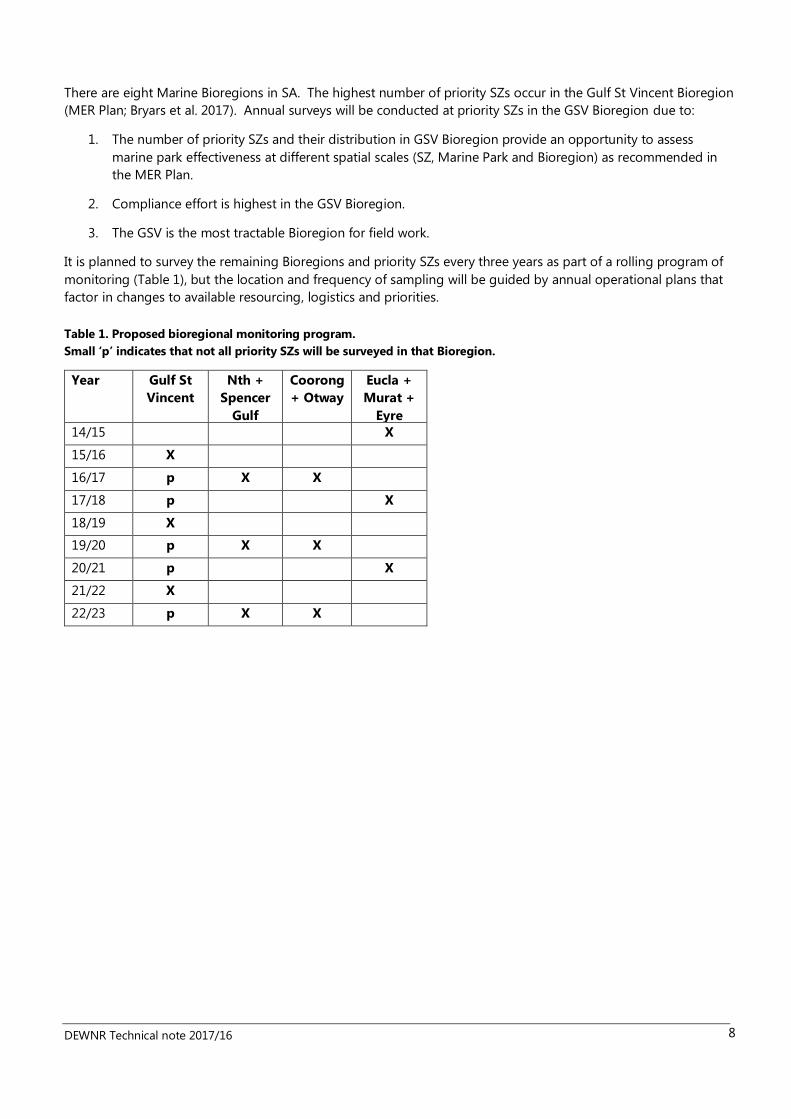
There are eight Marine Bioregions in SA. The highest number of priority SZs occur in the Gulf St Vincent Bioregion

(MER Plan; Bryars et al. 2017). Annual surveys will be conducted at priority SZs in the GSV Bioregion due to:

1. The number of priority SZs and their distribution in GSV Bioregion provide an opportunity to assess

marine park effectiveness at different spatial scales (SZ, Marine Park and Bioregion) as recommended in

the MER Plan.

2. Compliance effort is highest in the GSV Bioregion.

3. The GSV is the most tractable Bioregion for field work.

It is planned to survey the remaining Bioregions and priority SZs every three years as part of a rolling program of

monitoring (Table 1), but the location and frequency of sampling will be guided by annual operational plans that

factor in changes to available resourcing, logistics and priorities.

Table 1. Proposed bioregional monitoring program.

Small ‘p’ indicates that not all priority SZs will be surveyed in that Bioregion.

Year Gulf St

Vincent

Nth +

Spencer

Gulf

Coorong

+ Otway

Eucla +

Murat +

Eyre

14/15

X

15/16 X

16/17 p X X

17/18 p

X

18/19 X

19/20 p X X

20/21 p

X

21/22 X

22/23 p X X


4 Data processing and management

4.1 Overview

This section documents how the program manages data and information as a strategic asset of the Department

according to corporate standards and protocols, and in accordance with the Managing Environmental Knowledge

(MEK) Procedure and the DEWNR Information Management Framework (IMF).

The proper management of information is essential to ensuring that DEWNR effectively and efficiently meets a

number of legislative requirements such as those under the State Records Act 1997 and Freedom of Information Act

1991, as well as the Information Privacy Principles. The IMF defines the overarching rationale, principles and

lifecycle for the way DEWNR will manage the information it needs to achieve corporate goals and meet policy and

legislative requirements which include SAs’ declarations of ‘Open Data’ in 2013 and ‘digital by default’. A suite of

tools and guidelines in the MEK support achieving these goals.

The Marine Parks Program is committed to evidence based science and as such information collected by the

program needs to be managed consistently in line with DEWNRs data management policies. It also needs to

ensure that data and information collected as part of this program are available, accessible and well documented.

The program uses the MEK resources to meet these requirements.

There are a variety of data components that require management, these include:

Pre-dive data

Original datasheets

Photographs, including photoquadrat images (RLS method only) and photos to assist identification

Entered data (in databases and/or spreadsheets)

Processed photoquadrat data (in databases and/or spreadsheets)

Associated metadata

Data products

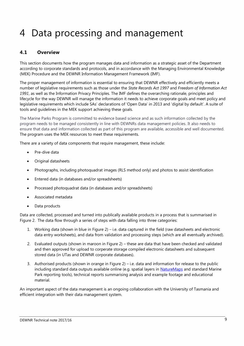
Data are collected, processed and turned into publically available products in a process that is summarised in

Figure 2. The data flow through a series of steps with data falling into three categories:

1. Working data (shown in blue in Figure 2) – i.e. data captured in the field (raw datasheets and electronic

data entry worksheets), and data from validation and processing steps (which are all eventually archived).

2. Evaluated outputs (shown in maroon in Figure 2) – these are data that have been checked and validated

and then approved for upload to corperate storage compiled electronic datasheets and subsequent

stored data (in UTas and DEWNR corporate databases).

3. Authorised products (shown in orange in Figure 2) – i.e. data and information for release to the public

including standard data outputs available online (e.g. spatial layers in NatureMaps and standard Marine

Park reporting tools), technical reports summarising analysis and example footage and educational

material.

An important aspect of the data management is an ongoing collaboration with the University of Tasmania and

efficient integration with their data management system.

https://data.environment.sa.gov.au/NatureMaps/Pages/default.aspx


Figure 2. Dataflow, data classification and data licencing within DEWNR’s diver UVC monitoring program.

Blue icons indicate working or draft data, maroon icons indicate outputs that have been evaluated and approved, and orange icons represent authorised products

ready for publishing. Dashed flow lines represent ‘aspirational’ items and products that are under development. At each stage where data is produced, a classification

is assigned and where appropriate, data is licenced and metadata records produced. (BST = Biological Survey Team, UTas = University of Tasmania, TBC = to be

created, FOUO = For Official Use Only, CC BY = Creative commons ‘Attribution’ licence).


4.2 Field preparation data

Field preparation data are generally limited to GPS marks for established sites, generally loaded to a GPS device

and in hardcopy, along with printed maps of the survey locations.

A summary of previously recorded species and abundances at established sites may also be useful.

4.3 Data capture

The appropriate format for recording survey data on the datasheets for the MPA and RLS methods is described in

detail by University of Tasmania (2010) and Reef Life Survey (2015), respectively. Additional points are:

Datasheets (Item 1, Figure 2) should contain data for a single site only to facilitate data processing and

storage.

The GPS marks for any new sites should be recorded on one of the survey datasheets and the dive log.

For the RLS method, the capture of photoquadrats (Item 2, Figure 2) is described in detail by Reef Life Survey

(2015). Additional points are:

The date and time on the camera should be checked prior to the dive as this will facilitate the processing

and curation of photoquadrat or identification photos.

4.4 Data processing and validation

4.4.1 Field validation

Data validation begins in the field and should be supervised by a dedicated data collator. At the conclusion of

each dive, each diver and the data collator should check that:

each datasheet includes the site name, date, depth, transect, diver name and buddy name

at least one datasheet includes the GPS mark (and waypoint number) for any new sites

at least one datasheet with fish data includes a visibility estimate

each species recorded has an abundance for at least one size class (method 1), the total abundance

(Method 2) or at least one quadrat (MPA Method 3)

any variations to the standard order for taking photoquadrats should be noted. The standard order would

see photos taken in the order of T2 then T1 towards the right hand end (when facing the shoreline), and

T3 then T4 towards the left hand end.

Each diver should check that:

all species names and abundance values are unambiguous and sufficiently legible to enable subsequent

coding and/or data entry.

any sample invertebrates brought to the surface, for which identifications cannot be confirmed by the dive

team, are photographed.

Datasheets should be rinsed in fresh water at the completion of each day.


4.4.2 Data entry

Data entry for MPA and RLS data should use the respective South Australian MS Excel templates supplied by UTas

for these methods.

Data entry is generally facilitated by using short codes for species (generally three letters but sometimes longer,

which are integrated into the data entry template). It is generally desirable for the individual divers to write the

codes onto the datasheets, to facilitate data entry by someone other than the diver who recorded the data. Care

should be taken, however, when using codes. The codes may vary a little between the RLS and MPA Programs,

between methods within the RLS Program, and also between local (state level) or global species lists. Most of the

codes are formed from the first letter of the genus concatenated with the first two letters of the specific epithet,

with additional letters from the specific epithet added where disambiguation is required. This disambiguation

results in some pairs of species for which coding can be error prone and for which particular care should be taken

during data entry and checking, e.g. Parequula melbournensis vs Paraplesiops meleagris, Petricia vernicina vs

Phasianella ventricosa, and Pleuroploca australasia vs Phasianella australis.

For RLS data, the depth field (decimal data type) has a critical second role, in that it is used to distinguish between

individual transects. For the SAMP-RLS method:

the integer part of the depth field should be used to record the depth of the survey. For resurveys of

established sites, the same value should be entered as for previous surveys, and should be independent of

variation associated with tide.

The decimal part of the depth field reflects the transect number, with ‘.0’ or no decimal used for T1

through to ‘.3’ for T4.

Size data

The MPA template has dedicated columns for the entry of size measurements and estimates.

For RLS, abalone and lobster sizes are entered into standard size classes in the ‘DATA’ worksheet of the RLS

template (Reef Life Survey 2015). In addition, the more precisely measured or estimated sizes can be entered into

the ‘NOTES’ worksheet of the RLS template, as follows:

1. Columns B to R from row 1 of the ‘DATA’ worksheet are copied to columns A to Q of the first row of

the ‘NOTES’ worksheet

2. Labels ‘Size’, ‘Estimate’ and ‘Sex’ are added in Row 1 of the columns R to T

3. Columns B to R from the relevant line of the ‘DATA’ worksheet are copied (paste special values and

number formats) to columns A to Q of the ‘NOTES’ worksheet for a number of rows corresponding

to the total abundance of abalone or lobster.

4. Columns R to T are populated with the size, estimate flag (1=estimated, blank = measured) and sex

(m, f or blank, always blank for abalone), respectively, for each individual abalone or lobster.

Following data entry, each sheet should be marked as ‘Entered’ and initialed by the person entering the

data. Datasheets should initially be collated in the same order as they are entered, as this will facilitate

spreadsheet data validation.

4.4.3 Spreadsheet data validation

Data entered into spreadsheets needs to be checked against the original datasheets. This is most effectively done

by two people working together, ideally one of whom is the diver who recorded the data. One person should read

out the data as presented on the sheet, while the other checks it against the spreadsheet.


The following actions should be taken depending on the error found:

If species codes or abundances (total or a size category) are wrong then they should be amended and

highlighted in yellow.

If one or two consecutive rows require deletion, then the rows from the spreadsheet can be deleted. If

there are more than two rows then the row below the block to be deleted should first be copied and

pasted back as values.

If rows need to be added, they should be added after the last line of valid data. If there are no rows

remaining in the template then rows can be copied and pasted from an earlier row (copy/paste rather

than fill down). The survey details (Columns B to O) can be copied and pasted (values and formats) from

an earlier row from the same survey. The new rows should be highlighted in green.

It is important to remember that the datasheets should be completed to the point of being a standalone

representation of the data. Therefore the datasheet should be modified for legibility where necessary and should

be updated with any post-field identifications from photos. It is also important to remember that in some cases

the datasheet may contain additional information that is not entered into the RLS template, e.g. sex information

for fish.

Once data entry has been validated against the data sheets, individual spreadsheets relating to the same survey

should be combined into a single, master spreadsheet. This should also collate and include any highlighted

additions to the species, site or diver worksheets.

A pivot table should then be used to check that there are data for all transects. This pivot table is already available

in the RLS data entry template. Pivot tables can also be used to check for data inconsistencies in site/position

information, between divers, depths/transects and blocks, as well as species lists for each diver.

4.4.4 Photoquadrat image processing

File sorting

Sorting of photoquadrat image files should occur as soon as possible after the completion of a diving day,

particularly if there is any variation from the standard order for taking photos. The standard order would see

photos taken in the order of T2 then T1 towards the right hand end (when facing the shoreline), and T3 then T4

towards the left hand end. If the photo image files are displayed in order of ‘Date taken’ and as icons/thumbnails

then it is easy to segregate the photos into transects. Additional aids like a photo of the datasheet or hand/fingers

(indicating transect no.) before each transect can also be helpful.

The naming convention for photos is as follows (Reef Life Survey 2015):

<site code>_<diver initials><depth>m<date (ddmmyy)><site name>

e.g. ENC7_JBB5.3m040314CarrickalingaHead

Note that the decimal component of the depth represents the transect number (with ‘.0’ for T1 incrementing by

0.1 for each transect up to 0.3 for T4).

A folder named according to this convention should be created for each RLS transect. Photoquadrat images

should be labelled as a batch for each transect, e.g. using the Windows rename function. This involves highlighting

all photos for one transect, leaving the cursor on the first of these highlighted quadrats, right-clicking and

selecting rename. This highlights the title of the first photoquadrat image and details should then be typed in (or

pasted from the previously copied folder name) with the file extension (.jpg) added. The rename function will

apply this naming convention to all PQs for that transect, adding suffices, (1), (2) etc., for disambiguation.


It is very important that the details in the photoquadrat image labels (site, diver, date) exactly match the details for

that survey in the RLS fish and invertebrate data entry worksheet to allow these two components to be matched

up in the RLS database.

The images should be backed up, at least until such time as they are received (via dropbox or external hard drive)

by the Reef Life Survey team at UTas.

Image interpretation

Image interpretation is a process whereby particular characteristics of the image (e.g. percentage cover of canopy-

forming macroalgae) are determined. There is generally a manual component to this process, but future

technologies may provide fully-automated methods.

The standard characteristics required for the MER Program are the percentage covers of benthic habitat classes

defined in a hierarchical classification. These are determined through a sample point overlay method where each

of the 20 images for a transect is sampled using 5 sample points, totaling 100 points for a full 50m transect (400

for a site). Identification of target groups (macroalgae, sessile invertebrates and substrate) is to the highest level

possible prior to aggregation to an appropriate level for analysis). Photoquadrat interpretation and analysis for the

MER Program is in its early stages and may further assessed and modified.

Comparison with MPA quadrat data

RLS photoquadrat data can be compared to the MPA method algal quadrats using a process outlined by Brook

and Bryars (2014). While RLS produces a ‘2D’ estimate of the percent cover of algae (generally canopy forming

species), the MPA method produces a ‘3D’ estimate of the percent cover of all species present by examining

individual layers of canopy. This multilayered estimate can be used to produce a percent cover range (ie from a

possible maximum and minimum ‘2D’ values that could be derived from the multilayered data), which can be used

to compare with RLS algal data.

4.4.5 Identification photo processing

Photos taken for the purpose of species identification should be retained and stored in a folder labeled using the

same convention as for the photoquadrats.

4.5 Post processing data management and storage

4.5.1 Datasheets, data submission, checking and storage

Data entry is often shared between DEWNR and UTas staff. Once data inputs have been checked and compiled as

per the instructions in the sections above, they are compiled into a single spreadsheet for submission to UTas for

storage in their national MPA/RLS databases. Datasheet originals are collated by site and region, scanned and

then archived by the respective organizations depending on who entered them. Scanned copies are retained by

both organisations. DEWNR archives datasheet scans on their corporate network.

Data submitted to UTas (Item 5, Figure 2) for upload to the national database undergoes further data checking as

per the RLS and MPA manuals (RLS and MPA methods manuals; Reef Life Survey 2015 and UTas 2010). Stored

data in the national database (Item 6, Figure 2) is made available to DEWNR on request. Ideally, DEWNR will

request a data update annually as soon as practical after the field season has concluded and the data entry and

validation process is complete.

Future plans for storage of the national database include the possibility of housing it through the Australian

Oceans Data Network (AODN) portal. This is currently under investigation and it is hoped data stored in this way

could be made available directly to contributing agencies such as DEWNR.

http://reeflifesurvey.com/wp-content/uploads/2015/07/NEW-Methods-Manual_150815.pdf


4.5.2 DEWNR storage of dive survey data

Annual (or when required) data exports from UTas will be stored and made available locally. The ‘flat’ standard

output table received from UTas (Item 7, Figure 2) will be processed through a custom MS Access database

(Item 8, Figure 2; also see Appendix C) to create a set of tables to be uploaded and stored on the corporate

system. These tables will likely take the form of Oracle database tables (e.g. a site table and a fish and

invertebrates table) which will provide for broad access to the data through the State Fauna and Flora ‘Supertable’

and a variety of other spatial and reporting tools (shown under ‘authorised products in Figure 2). The custom MS

Access database will also act as an interim storage solution for the data until such time an Oracle database can be

created and is stored on DEWNR’s corporate network.

4.6 Outputs and access

Outputs for the MER Program are mostly derived from the locally stored copy of the final dataset (held by UTas)

and include:

1. Data to support the MER Program (analysis and reporting)

2. Spatial layers

3. Metadata

4. Archived data

Some of these data outputs are currently under development and not yet available. It is also possible some details

may change during development.

4.6.1 Data to support MER Program analysis and reporting

Data stored in the national reef databases (managed by UTas) is available for analysis and reporting in two ways:

Via locally (SA) held output from the UTas databases, currently stored in a custom relational database

(Item 8, Figure 2, described in Appendix C) on the DEWNR network. Ultimately, the goal of the program is

to store this data in custom Oracle data tables (Item 9, Figure 2) which will have ‘live’ links to various

outputs.

Through a set of standardised reporting tools. It is envisaged that other reporting tools (linking directly to

stored data) will be developed. These may include metrics such as species presence, richness and biomass

by sanctuary zone and bioregion (inside and outside of protected areas).

4.6.2 Spatial layers

Spatial information will be available in the following forms:

Publicly via the State Fauna Supertable (which it is hoped will ultimately be linked to the network stored

Oracle data tables discussed above) and the ‘UVC sampling locations’ layer (currently under

development).

Internally available DEWNR data layers

4.6.3 Metadata

Formal metadata records for dive survey data mainly relate to the ‘Storage’ and ‘Outputs’ stages of the UVC

dataflow (Figure 2). The University of Tasmania maintains metadata for both the MPA and the RLS datasets.

Metadata for locally stored database (currently Item 8 in Figure 2) is available through the government’s

Location SA System (LMS; Dataset 2022).



4.6.4 Archived photoquadrats, identification photos and scanned data sheets

For each transect surveyed, a set of 20 algal photoquadrats is collected. These images are later used to derive

algal percent cover data. In addition, fish and invertebrate reference/identification images are collected by divers

as needed. Currently both image types are stored on duplicate backup drives (catalogued on on the DEWNR

network) and by the UTas (as part of their RLS program). These images, reference images in particular, often

provide a source of images for media and reporting.

Original data sheets are scanned and stored as a permanent reference and are held on DEWNR’s corporate drives

and by UTas.

4.7 Data classification and licencing

In 2013, the South Australian government committed to making government data ‘open’ and proactively

releasing government data to community, research and business organisations (SA Gov. Declaration of Open

Data). The Open Data Policy requires that data be freely available (published online where possible) and openly

licensed. Production and distribution of data in this way necessitates the classification and licencing of relevant

sets of data. DEWNR’s procedure for classifying, licensing and releasing data are based on the SA government’s

Information Security Management Framework.

Data and information collected by DEWNR is considered a valuable asset and as such, should be classified and

labelled according to the DEWNR classification guidelines. Classification establishes the confidentiality, integrity

and availability of each set of data or information. Data or information that is to be made available publicly (e.g.

on a web site, in a report, or on request) needs to be licenced according to the DEWNR licencing guidelines.

Diver survey ‘working data’ (Nos 1–4 in Figure 2) are all ‘transitional’ in nature, i.e. they are collection and data

preparation stages leading to the stored and reporting versions of the dataset. Although retained for reference,

these data are not intended for distribution and therefore can be considered as ‘not ready for public distribution

or posting. These data, including reference images and photoquadrats are archived. Future consideration will be

required in some cases (e.g. reference images deemed appropriate for promotional use) as the MER Program

expands and the team seek to further develop what can be made available.

Dive survey data stored within the national UTas reef database (No. 6 in Figure 2) are subject to licencing under

both DEWNR and UTas guidelines. Data in the locally held copy of the SA data are considered open data and

therefore classified for ‘Public distribution’. This data (eg. species presence, abundance and size) will eventually be

publically available via the ‘Fauna Supertable’. In exceptional cases where it is deemed necessary to delay release

or where partial data restriction is necessary (e.g. species sensitivity) a ‘data restriction category’ can be applied to

the relevant data. The Biological Survey Team authorise forwarding of data to UTas for upload to the database,

while restrictions will be implemented through application of the criteria in DEWNR’s information classification

guidelines.

Data for ‘Non-standard outputs’ (‘Analysis’ in Figure 2) is intended for internal use, that is, data analysis and the

production of outputs for use in Marine Parks reporting. This data therefore is considered as a transitional stage

for analysis and reporting outputs that ultimately form part of reports and other documents. It is therefore

considered to be ‘For Official Use Only’ based on the classification criteria. Reporting products (Nos 10–13)

derived from this data will undergo classification on a case by case basis, however, ultimately will generally be

classified for ‘Public’ distribution. In some instances where there is a justification, a caveat may be applied

delaying release of the document pending approval for release by the document authority.

Licencing of the data and products classified ‘Public’ will be applied based on DEWNR’s licencing guidelines and a

Creative Commons Attribution (CC BY) licence should be applied where possible. However, since much of the data

collected as part of the UVC survey program were done in collaboration with UTas (under a national research

project being conducted through the National Environmental Science Programmes; NESP, Marine Biodiversity

Hub) licencing of data products will in some instances need to comply with their licencing arrangements. While



https://digital.sa.gov.au/sites/default/files/content_files/policy/ISMF-v3F.pdf

http://www.ausgoal.gov.au/creative-commons

https://www.nespmarine.edu.au/project/project-c2-continental-scale-tracking-threats-shallow-australian-reef-ecosystems


data sharing and licencing arrangements are covered under this project, the UVC Program with UTas is ongoing

and has spanned multiple projects over many years. DEWNR is therefore seeking to set up a broader ‘data

memorandum of understanding’ maintained between the two agencies to manage data sharing and licencing

issues.


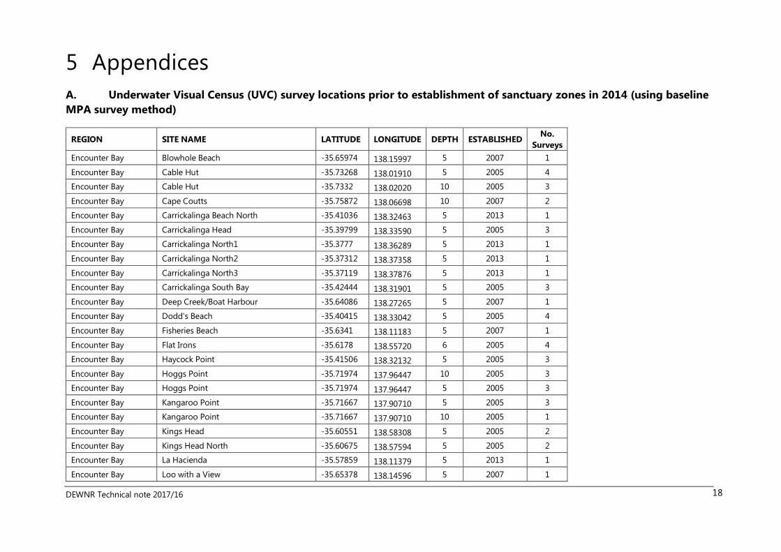
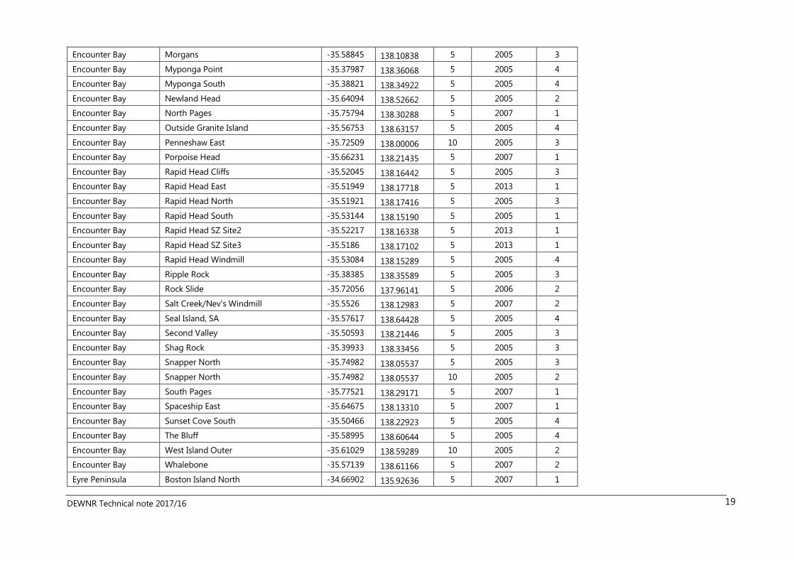
5 Appendices

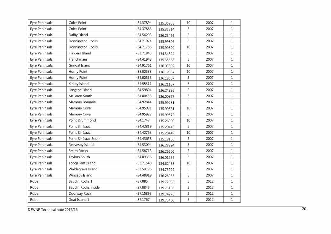
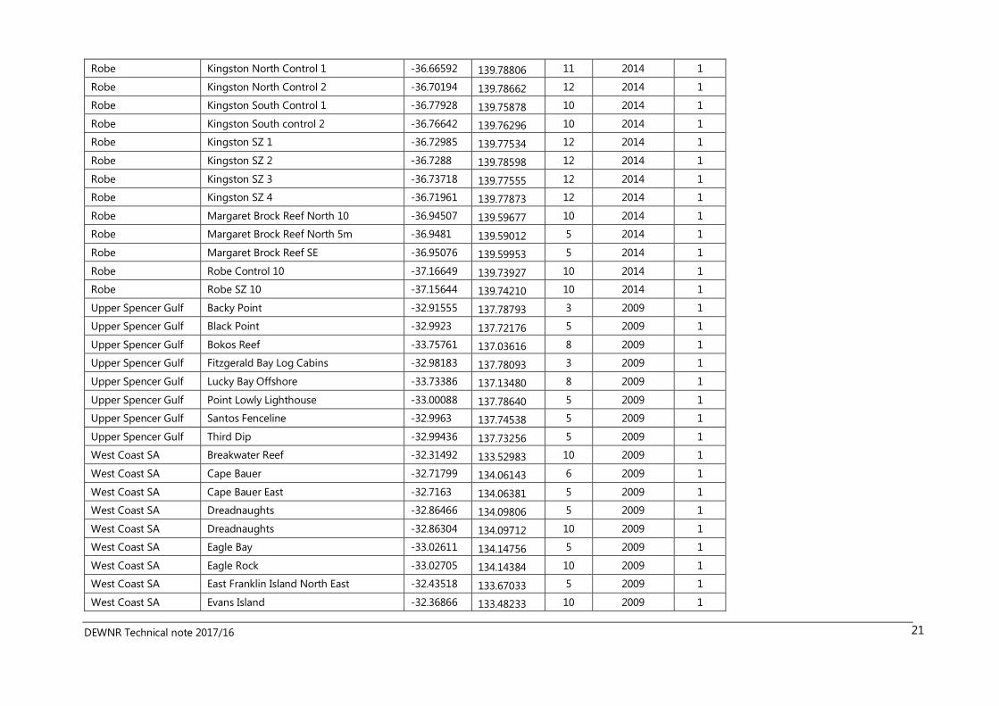
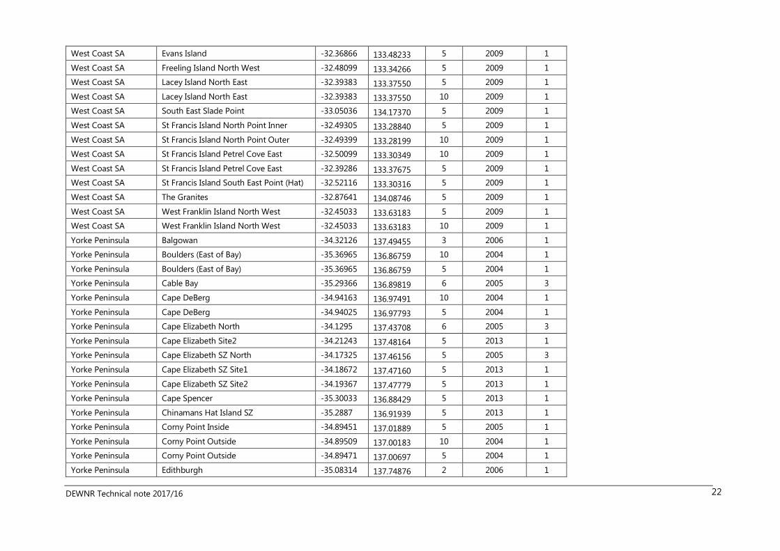
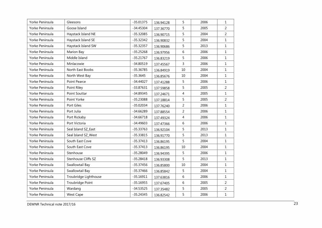
A. Underwater Visual Census (UVC) survey locations prior to establishment of sanctuary zones in 2014 (using baseline

MPA survey method)

REGION SITE NAME LATITUDE LONGITUDE DEPTH ESTABLISHED No.

Surveys

Encounter Bay Blowhole Beach -35.65974 138.15997 5 2007 1

Encounter Bay Cable Hut -35.73268 138.01910 5 2005 4

Encounter Bay Cable Hut -35.7332 138.02020 10 2005 3

Encounter Bay Cape Coutts -35.75872 138.06698 10 2007 2

Encounter Bay Carrickalinga Beach North -35.41036 138.32463 5 2013 1

Encounter Bay Carrickalinga Head -35.39799 138.33590 5 2005 3

Encounter Bay Carrickalinga North1 -35.3777 138.36289 5 2013 1



Encounter Bay Carrickalinga South Bay -35.42444 138.31901 5 2005 3

Encounter Bay Deep Creek/Boat Harbour -35.64086 138.27265 5 2007 1

Encounter Bay Dodd's Beach -35.40415 138.33042 5 2005 4

Encounter Bay Fisheries Beach -35.6341 138.11183 5 2007 1

Encounter Bay Flat Irons -35.6178 138.55720 6 2005 4

Encounter Bay Haycock Point -35.41506 138.32132 5 2005 3

Encounter Bay Hoggs Point -35.71974 137.96447 10 2005 3

Encounter Bay Hoggs Point -35.71974 137.96447 5 2005 3

Encounter Bay Kangaroo Point -35.71667 137.90710 5 2005 3

Encounter Bay Kangaroo Point -35.71667 137.90710 10 2005 1

Encounter Bay Kings Head -35.60551 138.58308 5 2005 2

Encounter Bay Kings Head North -35.60675 138.57594 5 2005 2

Encounter Bay La Hacienda -35.57859 138.11379 5 2013 1

Encounter Bay Loo with a View -35.65378 138.14596 5 2007 1


Encounter Bay Morgans -35.58845 138.10838 5 2005 3

Encounter Bay Myponga Point -35.37987 138.36068 5 2005 4

Encounter Bay Myponga South -35.38821 138.34922 5 2005 4

Encounter Bay Newland Head -35.64094 138.52662 5 2005 2

Encounter Bay North Pages -35.75794 138.30288 5 2007 1

Encounter Bay Outside Granite Island -35.56753 138.63157 5 2005 4

Encounter Bay Penneshaw East -35.72509 138.00006 10 2005 3

Encounter Bay Porpoise Head -35.66231 138.21435 5 2007 1

Encounter Bay Rapid Head Cliffs -35.52045 138.16442 5 2005 3

Encounter Bay Rapid Head East -35.51949 138.17718 5 2013 1

Encounter Bay Rapid Head North -35.51921 138.17416 5 2005 3

Encounter Bay Rapid Head South -35.53144 138.15190 5 2005 1

Encounter Bay Rapid Head SZ Site2 -35.52217 138.16338 5 2013 1

Encounter Bay Rapid Head SZ Site3 -35.5186 138.17102 5 2013 1

Encounter Bay Rapid Head Windmill -35.53084 138.15289 5 2005 4

Encounter Bay Ripple Rock -35.38385 138.35589 5 2005 3

Encounter Bay Rock Slide -35.72056 137.96141 5 2006 2

Encounter Bay Salt Creek/Nev's Windmill -35.5526 138.12983 5 2007 2

Encounter Bay Seal Island, SA -35.57617 138.64428 5 2005 4

Encounter Bay Second Valley -35.50593 138.21446 5 2005 3

Encounter Bay Shag Rock -35.39933 138.33456 5 2005 3

Encounter Bay Snapper North -35.74982 138.05537 5 2005 3

Encounter Bay Snapper North -35.74982 138.05537 10 2005 2

Encounter Bay South Pages -35.77521 138.29171 5 2007 1

Encounter Bay Spaceship East -35.64675 138.13310 5 2007 1

Encounter Bay Sunset Cove South -35.50466 138.22923 5 2005 4

Encounter Bay The Bluff -35.58995 138.60644 5 2005 4

Encounter Bay West Island Outer -35.61029 138.59289 10 2005 2

Encounter Bay Whalebone -35.57139 138.61166 5 2007 2

Eyre Peninsula Boston Island North -34.66902 135.92636 5 2007 1


Eyre Peninsula Coles Point -34.37894 135.35258 10 2007 1

Eyre Peninsula Coles Point -34.37883 135.35214 5 2007 1

Eyre Peninsula Dalby Island -34.56293 136.23466 5 2007 1

Eyre Peninsula Donnington Rocks -34.71974 135.99806 5 2007 1

Eyre Peninsula Donnington Rocks -34.71786 135.99899 10 2007 1

Eyre Peninsula Flinders Island -33.71843 134.54824 5 2007 1

Eyre Peninsula Frenchmans -34.41943 135.35858 5 2007 1

Eyre Peninsula Grindal Island -34.91761 136.03392 10 2007 1

Eyre Peninsula Horny Point -35.00533 136.19067 10 2007 1

Eyre Peninsula Horny Point -35.00533 136.19067 5 2007 1

Eyre Peninsula Kirkby Island -34.55311 136.21157 5 2007 1

Eyre Peninsula Langton Island -34.59804 136.24836 5 2007 1

Eyre Peninsula McLaren South -34.80433 136.00877 5 2007 1

Eyre Peninsula Memory Bommie -34.92844 135.99281 5 2007 1

Eyre Peninsula Memory Cove -34.95991 135.99861 10 2007 1

Eyre Peninsula Memory Cove -34.95927 135.99572 5 2007 1

Eyre Peninsula Point Drummond -34.1747 135.26000 10 2007 1

Eyre Peninsula Point Sir Isaac -34.42819 135.20443 5 2007 1

Eyre Peninsula Point Sir Isaac -34.42763 135.20449 10 2007 1

Eyre Peninsula Point Sir Isaac South -34.43658 135.19186 5 2007 1

Eyre Peninsula Reevesby Island -34.53094 136.28894 5 2007 1

Eyre Peninsula Smith Rocks -34.58713 136.26600 5 2007 1

Eyre Peninsula Taylors South -34.89336 136.01235 5 2007 1

Eyre Peninsula Topgallant Island -33.71548 134.62463 10 2007 1

Eyre Peninsula Waldegrave Island -33.59196 134.75929 5 2007 1

Eyre Peninsula Winceby Island -34.48919 136.28933 5 2007 1

Robe Baudin Rocks 1 -37.085 139.72065 5 2012 1

Robe Baudin Rocks inside -37.0845 139.73106 5 2012 1

Robe Doorway Rock -37.15893 139.74278 5 2012 1

Robe Goat Island 1 -37.1767 139.73460 5 2012 1


Robe Kingston North Control 1 -36.66592 139.78806 11 2014 1

Robe Kingston North Control 2 -36.70194 139.78662 12 2014 1

Robe Kingston South Control 1 -36.77928 139.75878 10 2014 1

Robe Kingston South control 2 -36.76642 139.76296 10 2014 1

Robe Kingston SZ 1 -36.72985 139.77534 12 2014 1

Robe Kingston SZ 2 -36.7288 139.78598 12 2014 1

Robe Kingston SZ 3 -36.73718 139.77555 12 2014 1

Robe Kingston SZ 4 -36.71961 139.77873 12 2014 1

Robe Margaret Brock Reef North 10 -36.94507 139.59677 10 2014 1

Robe Margaret Brock Reef North 5m -36.9481 139.59012 5 2014 1

Robe Margaret Brock Reef SE -36.95076 139.59953 5 2014 1

Robe Robe Control 10 -37.16649 139.73927 10 2014 1

Robe Robe SZ 10 -37.15644 139.74210 10 2014 1

Upper Spencer Gulf Backy Point -32.91555 137.78793 3 2009 1

Upper Spencer Gulf Black Point -32.9923 137.72176 5 2009 1

Upper Spencer Gulf Bokos Reef -33.75761 137.03616 8 2009 1

Upper Spencer Gulf Fitzgerald Bay Log Cabins -32.98183 137.78093 3 2009 1

Upper Spencer Gulf Lucky Bay Offshore -33.73386 137.13480 8 2009 1

Upper Spencer Gulf Point Lowly Lighthouse -33.00088 137.78640 5 2009 1

Upper Spencer Gulf Santos Fenceline -32.9963 137.74538 5 2009 1

Upper Spencer Gulf Third Dip -32.99436 137.73256 5 2009 1

West Coast SA Breakwater Reef -32.31492 133.52983 10 2009 1

West Coast SA Cape Bauer -32.71799 134.06143 6 2009 1

West Coast SA Cape Bauer East -32.7163 134.06381 5 2009 1

West Coast SA Dreadnaughts -32.86466 134.09806 5 2009 1

West Coast SA Dreadnaughts -32.86304 134.09712 10 2009 1

West Coast SA Eagle Bay -33.02611 134.14756 5 2009 1

West Coast SA Eagle Rock -33.02705 134.14384 10 2009 1

West Coast SA East Franklin Island North East -32.43518 133.67033 5 2009 1

West Coast SA Evans Island -32.36866 133.48233 10 2009 1


West Coast SA Evans Island -32.36866 133.48233 5 2009 1

West Coast SA Freeling Island North West -32.48099 133.34266 5 2009 1

West Coast SA Lacey Island North East -32.39383 133.37550 5 2009 1

West Coast SA Lacey Island North East -32.39383 133.37550 10 2009 1

West Coast SA South East Slade Point -33.05036 134.17370 5 2009 1

West Coast SA St Francis Island North Point Inner -32.49305 133.28840 5 2009 1

West Coast SA St Francis Island North Point Outer -32.49399 133.28199 10 2009 1

West Coast SA St Francis Island Petrel Cove East -32.50099 133.30349 10 2009 1

West Coast SA St Francis Island Petrel Cove East -32.39286 133.37675 5 2009 1

West Coast SA St Francis Island South East Point (Hat) -32.52116 133.30316 5 2009 1

West Coast SA The Granites -32.87641 134.08746 5 2009 1

West Coast SA West Franklin Island North West -32.45033 133.63183 5 2009 1

West Coast SA West Franklin Island North West -32.45033 133.63183 10 2009 1

Yorke Peninsula Balgowan -34.32126 137.49455 3 2006 1

Yorke Peninsula Boulders (East of Bay) -35.36965 136.86759 10 2004 1

Yorke Peninsula Boulders (East of Bay) -35.36965 136.86759 5 2004 1

Yorke Peninsula Cable Bay -35.29366 136.89819 6 2005 3

Yorke Peninsula Cape DeBerg -34.94163 136.97491 10 2004 1

Yorke Peninsula Cape DeBerg -34.94025 136.97793 5 2004 1

Yorke Peninsula Cape Elizabeth North -34.1295 137.43708 6 2005 3

Yorke Peninsula Cape Elizabeth Site2 -34.21243 137.48164 5 2013 1

Yorke Peninsula Cape Elizabeth SZ North -34.17325 137.46156 5 2005 3

Yorke Peninsula Cape Elizabeth SZ Site1 -34.18672 137.47160 5 2013 1

Yorke Peninsula Cape Elizabeth SZ Site2 -34.19367 137.47779 5 2013 1

Yorke Peninsula Cape Spencer -35.30033 136.88429 5 2013 1

Yorke Peninsula Chinamans Hat Island SZ -35.2887 136.91939 5 2013 1

Yorke Peninsula Corny Point Inside -34.89451 137.01889 5 2005 1

Yorke Peninsula Corny Point Outside -34.89509 137.00183 10 2004 1

Yorke Peninsula Corny Point Outside -34.89471 137.00697 5 2004 1

Yorke Peninsula Edithburgh -35.08314 137.74876 2 2006 1


Yorke Peninsula Gleesons -35.01375 136.94128 5 2006 1

Yorke Peninsula Goose Island -34.45304 137.36770 5 2005 2

Yorke Peninsula Haystack Island NE -35.32085 136.90715 5 2004 2

Yorke Peninsula Haystack Island SE -35.32342 136.90832 5 2004 1

Yorke Peninsula Haystack Island SW -35.32357 136.90686 5 2013 1

Yorke Peninsula Marion Bay -35.25268 136.97956 6 2006 1

Yorke Peninsula Middle Island -35.21767 136.83219 5 2006 1

Yorke Peninsula Minlacowie -34.80519 137.45567 3 2006 1

Yorke Peninsula North East Boobs -35.36785 136.84919 10 2004 1

Yorke Peninsula North West Bay -35.3645 136.85676 10 2004 1

Yorke Peninsula Point Pearce -34.44027 137.41288 5 2006 1

Yorke Peninsula Point Riley -33.87631 137.59858 5 2005 2

Yorke Peninsula Point Souttar -34.89345 137.24671 4 2005 1

Yorke Peninsula Point Yorke -35.23088 137.18814 5 2005 2

Yorke Peninsula Port Giles -35.02034 137.76240 2 2006 1

Yorke Peninsula Port Julia -34.66289 137.88554 2 2006 1

Yorke Peninsula Port Rickaby -34.66718 137.49324 4 2006 1

Yorke Peninsula Port Victoria -34.49603 137.47366 6 2006 1

Yorke Peninsula Seal Island SZ_East -35.33763 136.92104 5 2013 1

Yorke Peninsula Seal Island SZ_West -35.33815 136.91770 5 2013 1

Yorke Peninsula South East Cove -35.37413 136.86195 5 2004 1

Yorke Peninsula South East Cove -35.37413 136.86195 10 2004 1

Yorke Peninsula Stenhouse -35.28049 136.94395 5 2006 1

Yorke Peninsula Stenhouse Cliffs SZ -35.28418 136.93308 5 2013 1

Yorke Peninsula Swallowtail Bay -35.37456 136.85800 10 2004 1

Yorke Peninsula Swallowtail Bay -35.37466 136.85842 5 2004 1

Yorke Peninsula Troubridge Lighthouse -35.16911 137.63816 6 2006 1

Yorke Peninsula Troubridge Point -35.16955 137.67405 6 2005 2

Yorke Peninsula Wardang -34.53525 137.35482 5 2005 2

Yorke Peninsula West Cape -35.24345 136.82542 5 2006 1


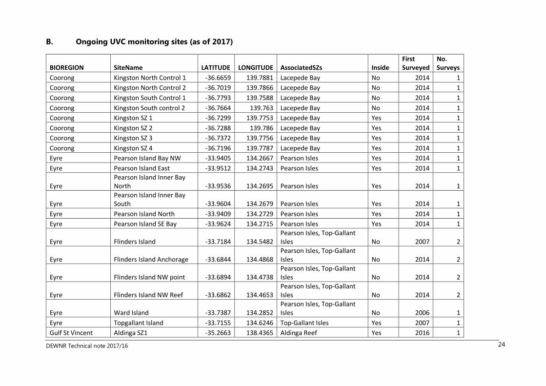
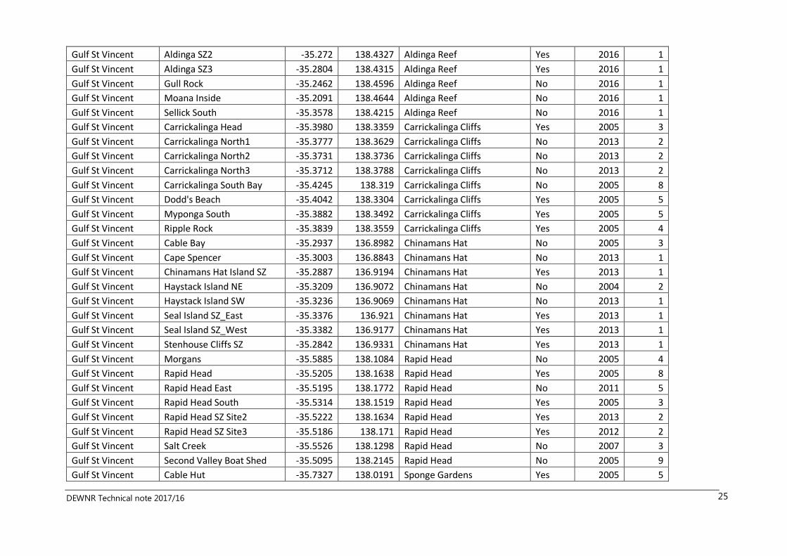
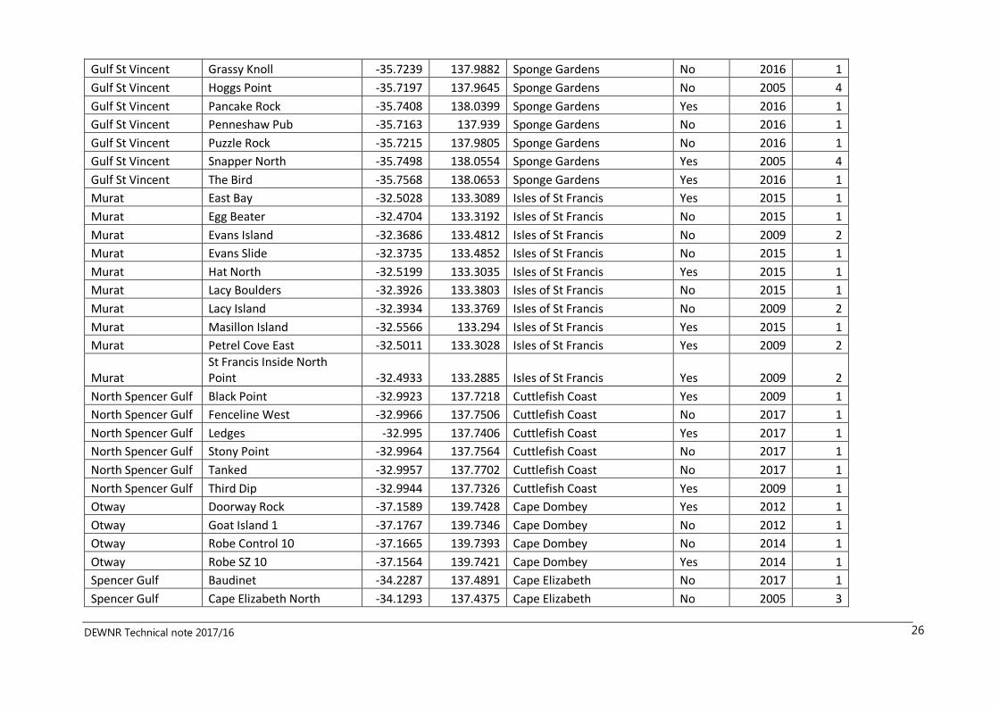
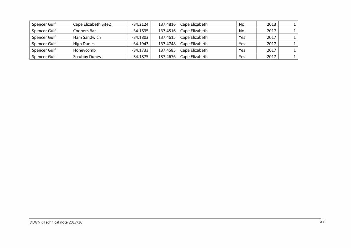
B. Ongoing UVC monitoring sites (as of 2017)

BIOREGION SiteName LATITUDE LONGITUDE AssociatedSZs Inside First Surveyed

No. Surveys

Coorong Kingston North Control 1 -36.6659 139.7881 Lacepede Bay No 2014 1

Coorong Kingston North Control 2 -36.7019 139.7866 Lacepede Bay No 2014 1

Coorong Kingston South Control 1 -36.7793 139.7588 Lacepede Bay No 2014 1

Coorong Kingston South control 2 -36.7664 139.763 Lacepede Bay No 2014 1

Coorong Kingston SZ 1 -36.7299 139.7753 Lacepede Bay Yes 2014 1




Eyre Pearson Island Bay NW -33.9405 134.2667 Pearson Isles Yes 2014 1

Eyre Pearson Island East -33.9512 134.2743 Pearson Isles Yes 2014 1

Eyre Pearson Island Inner Bay North -33.9536 134.2695 Pearson Isles Yes 2014 1

Eyre Pearson Island Inner Bay South -33.9604 134.2679 Pearson Isles Yes 2014 1

Eyre Pearson Island North -33.9409 134.2729 Pearson Isles Yes 2014 1

Eyre Pearson Island SE Bay -33.9624 134.2715 Pearson Isles Yes 2014 1

Eyre Flinders Island -33.7184 134.5482 Pearson Isles, Top-Gallant Isles No 2007 2

Eyre Flinders Island Anchorage -33.6844 134.4868 Pearson Isles, Top-Gallant Isles No 2014 2

Eyre Flinders Island NW point -33.6894 134.4738 Pearson Isles, Top-Gallant Isles No 2014 2

Eyre Flinders Island NW Reef -33.6862 134.4653 Pearson Isles, Top-Gallant Isles No 2014 2

Eyre Ward Island -33.7387 134.2852 Pearson Isles, Top-Gallant Isles No 2006 1

Eyre Topgallant Island -33.7155 134.6246 Top-Gallant Isles Yes 2007 1

Gulf St Vincent Aldinga SZ1 -35.2663 138.4365 Aldinga Reef Yes 2016 1




Gulf St Vincent Gull Rock -35.2462 138.4596 Aldinga Reef No 2016 1

Gulf St Vincent Moana Inside -35.2091 138.4644 Aldinga Reef No 2016 1

Gulf St Vincent Sellick South -35.3578 138.4215 Aldinga Reef No 2016 1

Gulf St Vincent Carrickalinga Head -35.3980 138.3359 Carrickalinga Cliffs Yes 2005 3

Gulf St Vincent Carrickalinga North1 -35.3777 138.3629 Carrickalinga Cliffs No 2013 2



Gulf St Vincent Carrickalinga South Bay -35.4245 138.319 Carrickalinga Cliffs No 2005 8

Gulf St Vincent Dodd's Beach -35.4042 138.3304 Carrickalinga Cliffs Yes 2005 5

Gulf St Vincent Myponga South -35.3882 138.3492 Carrickalinga Cliffs Yes 2005 5

Gulf St Vincent Ripple Rock -35.3839 138.3559 Carrickalinga Cliffs Yes 2005 4

Gulf St Vincent Cable Bay -35.2937 136.8982 Chinamans Hat No 2005 3

Gulf St Vincent Cape Spencer -35.3003 136.8843 Chinamans Hat No 2013 1

Gulf St Vincent Chinamans Hat Island SZ -35.2887 136.9194 Chinamans Hat Yes 2013 1

Gulf St Vincent Haystack Island NE -35.3209 136.9072 Chinamans Hat No 2004 2

Gulf St Vincent Haystack Island SW -35.3236 136.9069 Chinamans Hat No 2013 1

Gulf St Vincent Seal Island SZ_East -35.3376 136.921 Chinamans Hat Yes 2013 1

Gulf St Vincent Seal Island SZ_West -35.3382 136.9177 Chinamans Hat Yes 2013 1

Gulf St Vincent Stenhouse Cliffs SZ -35.2842 136.9331 Chinamans Hat Yes 2013 1

Gulf St Vincent Morgans -35.5885 138.1084 Rapid Head No 2005 4

Gulf St Vincent Rapid Head -35.5205 138.1638 Rapid Head Yes 2005 8

Gulf St Vincent Rapid Head East -35.5195 138.1772 Rapid Head No 2011 5

Gulf St Vincent Rapid Head South -35.5314 138.1519 Rapid Head Yes 2005 3

Gulf St Vincent Rapid Head SZ Site2 -35.5222 138.1634 Rapid Head Yes 2013 2

Gulf St Vincent Rapid Head SZ Site3 -35.5186 138.171 Rapid Head Yes 2012 2

Gulf St Vincent Salt Creek -35.5526 138.1298 Rapid Head No 2007 3

Gulf St Vincent Second Valley Boat Shed -35.5095 138.2145 Rapid Head No 2005 9

Gulf St Vincent Cable Hut -35.7327 138.0191 Sponge Gardens Yes 2005 5


Gulf St Vincent Grassy Knoll -35.7239 137.9882 Sponge Gardens No 2016 1

Gulf St Vincent Hoggs Point -35.7197 137.9645 Sponge Gardens No 2005 4

Gulf St Vincent Pancake Rock -35.7408 138.0399 Sponge Gardens Yes 2016 1

Gulf St Vincent Penneshaw Pub -35.7163 137.939 Sponge Gardens No 2016 1

Gulf St Vincent Puzzle Rock -35.7215 137.9805 Sponge Gardens No 2016 1

Gulf St Vincent Snapper North -35.7498 138.0554 Sponge Gardens Yes 2005 4

Gulf St Vincent The Bird -35.7568 138.0653 Sponge Gardens Yes 2016 1

Murat East Bay -32.5028 133.3089 Isles of St Francis Yes 2015 1

Murat Egg Beater -32.4704 133.3192 Isles of St Francis No 2015 1

Murat Evans Island -32.3686 133.4812 Isles of St Francis No 2009 2

Murat Evans Slide -32.3735 133.4852 Isles of St Francis No 2015 1

Murat Hat North -32.5199 133.3035 Isles of St Francis Yes 2015 1

Murat Lacy Boulders -32.3926 133.3803 Isles of St Francis No 2015 1

Murat Lacy Island -32.3934 133.3769 Isles of St Francis No 2009 2

Murat Masillon Island -32.5566 133.294 Isles of St Francis Yes 2015 1

Murat Petrel Cove East -32.5011 133.3028 Isles of St Francis Yes 2009 2

Murat St Francis Inside North Point -32.4933 133.2885 Isles of St Francis Yes 2009 2

North Spencer Gulf Black Point -32.9923 137.7218 Cuttlefish Coast Yes 2009 1

North Spencer Gulf Fenceline West -32.9966 137.7506 Cuttlefish Coast No 2017 1

North Spencer Gulf Ledges -32.995 137.7406 Cuttlefish Coast Yes 2017 1

North Spencer Gulf Stony Point -32.9964 137.7564 Cuttlefish Coast No 2017 1

North Spencer Gulf Tanked -32.9957 137.7702 Cuttlefish Coast No 2017 1

North Spencer Gulf Third Dip -32.9944 137.7326 Cuttlefish Coast Yes 2009 1

Otway Doorway Rock -37.1589 139.7428 Cape Dombey Yes 2012 1

Otway Goat Island 1 -37.1767 139.7346 Cape Dombey No 2012 1

Otway Robe Control 10 -37.1665 139.7393 Cape Dombey No 2014 1

Otway Robe SZ 10 -37.1564 139.7421 Cape Dombey Yes 2014 1

Spencer Gulf Baudinet -34.2287 137.4891 Cape Elizabeth No 2017 1

Spencer Gulf Cape Elizabeth North -34.1293 137.4375 Cape Elizabeth No 2005 3


Spencer Gulf Cape Elizabeth Site2 -34.2124 137.4816 Cape Elizabeth No 2013 1

Spencer Gulf Coopers Bar -34.1635 137.4516 Cape Elizabeth No 2017 1

Spencer Gulf Ham Sandwich -34.1803 137.4615 Cape Elizabeth Yes 2017 1

Spencer Gulf High Dunes -34.1943 137.4748 Cape Elizabeth Yes 2017 1

Spencer Gulf Honeycomb -34.1733 137.4585 Cape Elizabeth Yes 2017 1

Spencer Gulf Scrubby Dunes -34.1875 137.4676 Cape Elizabeth Yes 2017 1


C. Importing data from the University of Tasmania (UTas) national database

A set of standardised tables is taken from the national database for import to DEWNR’s UVC dataset, at any time

that DEWNR require updates as a result of changes to the SA component of the national dataset (e.g. following

new surveys, or following any corrections to the data). In particular, this would occur as soon as practical after

annual surveys are complete and the data has been uploaded to the UTas databases. Regular (annual) imports

would include the following tables:

Combined RLS and MPA fish and mobile invertebrate data extract

UTas species table

RLS photoquadrat data

In addition, a ‘one off’ import of the baseline MPA algal quadrat data is required. This import would be repeated

only if further surveys using the MPA method are carried out in the future. Due to the differing needs of RLS and

DEWNR, a mechanism for storage and import of lobster and abalone size data is still being developed (currently

stored locally in parallel with the processes described here).

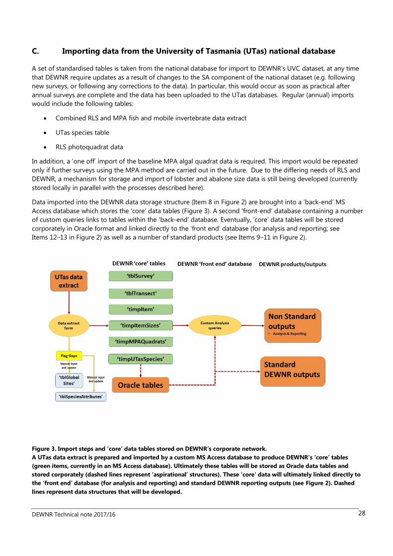
Data imported into the DEWNR data storage structure (Item 8 in Figure 2) are brought into a ‘back-end’ MS

Access database which stores the ‘core’ data tables (Figure 3). A second ‘front-end’ database containing a number

of custom queries links to tables within the ‘back-end’ database. Eventually, ‘core’ data tables will be stored

corporately in Oracle format and linked directly to the ‘front end’ database (for analysis and reporting; see

Items 12–13 in Figure 2) as well as a number of standard products (see Items 9–11 in Figure 2).

Figure 3. Import steps and ‘core’ data tables stored on DEWNR’s corporate network.

A UTas data extract is prepared and imported by a custom MS Access database to produce DEWNR’s ‘core’ tables

(green items, currently in an MS Access database). Ultimately these tables will be stored as Oracle data tables and

stored corporately (dashed lines represent ‘aspirational’ structures). These ‘core’ data will ultimately linked directly to

the ‘front end’ database (for analysis and reporting) and standard DEWNR reporting outputs (see Figure 2). Dashed

lines represent data structures that will be developed.


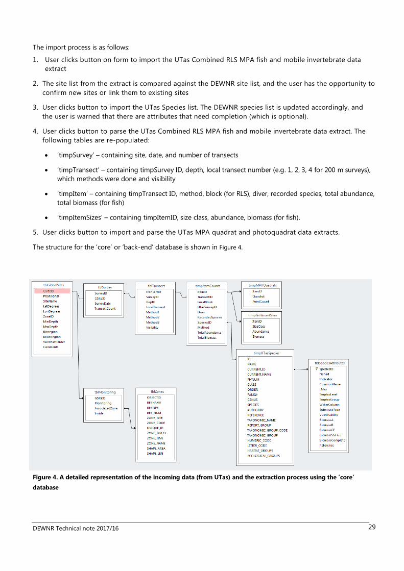
The import process is as follows:

1. User clicks button on form to import the UTas Combined RLS MPA fish and mobile invertebrate data

extract

2. The site list from the extract is compared against the DEWNR site list, and the user has the opportunity to

confirm new sites or link them to existing sites

3. User clicks button to import the UTas Species list. The DEWNR species list is updated accordingly, and

the user is warned that there are attributes that need completion (which is optional).

4. User clicks button to parse the UTas Combined RLS MPA fish and mobile invertebrate data extract. The

following tables are re-populated:

‘timpSurvey’ – containing site, date, and number of transects

‘timpTransect’ – containing timpSurvey ID, depth, local transect number (e.g. 1, 2, 3, 4 for 200 m surveys),

which methods were done and visibility

‘timpItem’ – containing timpTransect ID, method, block (for RLS), diver, recorded species, total abundance,

total biomass (for fish)

‘timpItemSizes’ – containing timpItemID, size class, abundance, biomass (for fish).

5. User clicks button to import and parse the UTas MPA quadrat and photoquadrat data extracts.

The structure for the ‘core’ or ‘back-end’ database is shown in Figure 4.

Figure 4. A detailed representation of the incoming data (from UTas) and the extraction process using the ’core’

database


6 References Baron, RM, Lance, KB & Spieler, RE 2004, Characterisation of the marine fish assemblage associated with

nearshore hard bottom of Broward County, Florid, USA. Estuarine, Coastal and Shelf Science. 60: 431–443.

Barrett, NS, Edgar, GJ, Buxton, CD & Haddon, M 2007, Changes in fish assemblages following 10 years of

protection in Tasmanian marine protected areas, Journal of Experimental Marine Biology and Ecology, vol. 345,

pp. 141–157.

Brook, J and Bryars, S 2014, Condition status of selected subtidal reefs on the Fleurieu Peninsula. Report to the

Adelaide and Mount Lofty Ranges Natural Resources Management Board. J Diversity Pty Ltd, Adelaide.

Bryars, S 2013, Monitoring fishes and invertebrates inside South Australia’s marine parks network: a scoping

document for establishing baselines and guiding an ongoing monitoring program. Report to the Marine Parks

Monitoring, Evaluation and Reporting Program within the Department of Environment, Water and Natural

Resources. Dr Simon Richard Bryars, Adelaide.

Bryars, S., Brook, J., Meakin, C., McSkimming, C., Eglinton, Y., Morcom, R., Wright, A. and Page, B. 2016, Baseline

and predicted changes for the Encounter Marine Park, DEWNR Technical report 2016/25, Government of South

Australia, through Department of Environment, Water and Natural Resources, Adelaide

Bryars, S, Page, B, Waycott, M, Brock, D and Wright, A, 2017, South Australian Marine Parks Monitoring, Evaluation

and Reporting Plan, DEWNR Technical report 2017/05, Government of South Australia, through Department of

Environment, Water and Natural Resources, Adelaide

Delean, S. unpublished report, Detecting changes in biodiversity indicators in South Australia’s Marine Parks. Draft

report to the Department of Environment, Water and Natural Resources, South Australia. University of Adelaide,

Adelaide.

Edgar, G.J. and Barrett, N.S. 1999, Effects of the declaration of marine reserves on Tasmanian reef fishes,

invertebrates and plants. Journal of Experimental Marine Biology and Ecology, 242: 107–144.

Edgar, G.J., Barrett, N.S., Brook, J., McDonald, B. and Bloomfield, A., 2006,, Ecosystem monitoring inside and

outside proposed Sanctuary Zones with the Encounter Marine Park – 2005 baseline surveys., Tasmanian

Aquaculture and Fisheries Institute. Hobart Tas.

Edgar GJ & Stuart-Smith RD. 2009. Ecological effects of marine protected areas on rocky reef communities: a

continental-scale analysis. Marine Ecology Progress Series. 2009; 388:51–62.

Girolamo, M. D. and Mazzoldi, 2001. The application of visual census on Mediterranean rocky habitats. Marine

Environmental Research 51: 1-16.

Holmes, TH, Wilson, SK, Travers, MJ, Langlois, TJ, Evans, RD, Moore, GI, Douglas, RA, Shedrawi, G, Harvey, ES &

Hickey, K, 2013. A comparison of visual- and stereo-video based fish community assessment methods in tropical

and temperate marine waters of Western Australia. Limnology and oceanography: Methods 11: 337-350.

Reef Life Survey 2015, Standardised survey procedures for monitoring rocky & coral reef ecological communities.

Reef Life Survey Program.

Soler, GA, Edgar, GJ, Thomson RJ, Kininmonth, S, Campbell, SJ, Dawson, TP, Barrett, NS, Bernard, ATF, Galván, DE,

Willis, TJ, Alexander, TJ & Stuart-Smith RD 2015, Reef fishes at all trophic levels respond positively to effective

marine protected areas. PLoS ONE 10(10): e0140270. doi:10.1371/journal.pone.0140270.

Stuart-Smith, RD, Edgar, GJ, Barrett, NS, Bates, AE, Baker, SC, Bax, NJ, Becerro, MA, Blanchard, JL, Brock, DJ, Clark,

GF, Davis, TR, Day, PB, Duffy, JD, Holmes, TH, Howe, S, Jordan, A, Kininmonth, S, Knott, NA, Lefcheck, JS, Ling, SD,


Parr, A, Strain, E, Sweatman, H & Thomson, R. 2017. Assessing national biodiversity trends for rocky and coral reefs

through the integration of Citizen Science and scientific monitoring Programs. Bioscience. 67 (2):134-146.

University of Tasmania 2010, Marine Biodiversity Database Documents. Unpublished report.

Permissive Licence ©State of South Australia through the Department of Environment, Water and Natural

Resources. Apart from fair dealings and other uses permitted by the Copyright Act 1968

(Cth), no part of this publication may be reproduced, published, communicated,

transmitted, modified or commercialised without the prior written approval of the

Department of Environment, Water and Natural Resources.

Written requests for permission should be addressed to:

Communications Manager


GPO Box 1047 Adelaide SA 5001

Disclaimer While reasonable efforts have been made to ensure the contents of this publication are

factually correct, the Department of Environment, Water and Natural Resources makes no

representations and accepts no responsibility for the accuracy, completeness or fitness for

any particular purpose of the contents, and shall not be liable for any loss or damage that

may be occasioned directly or indirectly through the use of or reliance on the contents of

this publication. Reference to any company, product or service in this publication should

not be taken as a Departmental endorsement of the company, product or service.

© Department of Environment, Water and Natural Resources | June 2017 | FIS 94369