t

Underwater Acoustic Imaging: Rapid Signal Processing

David G. Blair and Ian S.F. Jones

DSTO-TN-0098

APPROVED FOR PUBLIC RELEASE

© Commonwealth of Australia

DEPARTMENT OF DEFENCE

DEFENCE SCIENCE AND TECHNOLOGY ORGANISATION

Underwater Acoustic Imaging: Rapid Signal Processing

David G. Blair and Ian S. F. Jones

Maritime Operations Division Aeronautical and Maritime Research Laboratory

DSTO-TN-0098

ABSTRACT

An innovation program to develop an underwater acoustic imaging system able to resolve objects down to millimetre resolution in turbid waters is under way. The defence need is for the identification of minelike objects. This report reviews options for the signal processing or beamforming stage of the program. An image consisting of 3xl09 voxels (volume pixels) could be formed by a summation of the voltages from 4000 sensor elements, each taken from the element's voltage stream at the appropriate time. With a suitable allowance (factor of 9) for calculating the time delays, it appears at first sight that 9xl.2xl013 operations would be required. The problem is to calculate a three-dimensional image of adequate quality in the shortest time at the least cost. A hierarchical structure of options is developed in an attempt to capture all possibilities. At the top level, three approaches are identified. First, the use of appropriate hardware, such as computers with parallelism. Second, a reduction in the number of operations (a 'software' solution). And third, the defining of a suitable reduced goal, which appears to come down to the imaging of a subvolume of the original volume that contains the object of interest. Each of these three approaches is divided into suboptions; these are discussed in detail to bring out difficulties and advantages.

19980706 155 RELEASE LIMITATION

Approved for public release

DEPARTMENT OF DEFENCE +

DEFENCE SCIENCE AND TECHNOLOGY ORGANISATION

JgHO QUALITY INSPECTED 1

Published by

DSTO Aeronautical and Maritime Research Laboratory PO Box 4331 Melbourne Victoria 3001 Australia

Telephone: (03) 9626 7000 Fax: (03)9626 7999 © Commonwealth of Australia 1998 AR-010-280 April 1998

APPROVED FOR PUBLIC RELEASE

Underwater Acoustic Imaging: Rapid Signal Processing

Executive Summary

As part of Australian defence policy to counter sea mines, the need has been recognised for an enhanced capability to identify objects that have been classified as minelike. Because the medium is often too turbid for optical methods to work, DSTO is working with Australian industry to develop a high-resolution underwater acoustic (sonar) imaging system, intended to 'see' detail of size 1 mm at a range of 1 m. The system has successfully passed the concept demonstrator stage.

This report reviews options for the signal processing phase of the innovation plan. The processing for the present design involves, for each of 3 x 109 volume pixels (voxels), a summation of 4000 voltages, one from each sensor element, taken from that element's voltage stream at the appropriate time. It therefore appears that at least 1 ■ 2 x 1013 operations are required; for a combination of reasons, the expected figure becomes nine times that number. Thus a 1 Gflops computer (109 floating point operations per second) would require 30 hours to produce the image, unacceptably long by far. (Note also that further overheads are required in a practical computer, yielding yet another factor of say 2.)

However it may be possible to greatly reduce the computation time needed. Thus the problem is to determine how to calculate the full three-dimensional image in the shortest time or, if that time is too long to be useful, to develop the best strategy for obtaining an image over a reduced volume embracing the object of interest.

A hierarchical structure of options is developed in an attempt to capture all possibilities. At the top level, three approaches are identified. First, the use of appropriate hardware, such as computers with parallelism, or the use of an optical analogue. Second, a reduction in the number of operations (a 'software' solution). And third, the defining of a suitable reduced goal, which appears to come down to the imaging of a subvolume of the original volume. Each of these three approaches is subdivided into suboptions; these are discussed in detail to bring out difficulties and advantages.

In the third approach, one is likely to aim for a subvolume that is a slice about the front surface of the target, restricted further to an angular sector chosen from prior information as containing the strongest clues to mine identification. This approach can yield a dramatic reduction in computing time, but it is not clear that it reliably yields the subvolume (in terms both of the range and of the direction) that is needed for mine identification.

Within the third approach, a method that apparently images all the front surface of the target in a usefully short time is described.

Contents

1. BACKGROUND *

2. PHILOSOPHY 1

3. THE PROBLEM • 1

3.1 The System and its Parameters * 3.2 Beamforming: Theory 3

3.3 Computation Times 3

3.3.1 Dechirping; the Quadrature Part 3 3.3.2 Beamforming Proper 4

4. BROAD APPROACHES 4

5. THE HARDWARE APPROACH 5

5.1 General jj 5.2 Serial Computer 5

5.3 Parallelism * 5.3.1 Approaches within Parallelism 6

5.3.2 Treating Elements in Parallel 7 5.3.3 Other Approaches with Parallelism 7

5.4 Analogues of the Reconstruction 8

6. THE SOFTWARE APPROACH: REDUCING THE NUMBER OF OPERATIONS9 6.1 Background 9

6.2 Approaches 9 6.3 Efficient Calculation of Individual Addresses 10 6.4 Avoiding Repeated Calculations 10

6.4.1 General 10

6.4.2 Repetition of Relative Address 12 6.4.2.1 Definition and Potential 12 6.4.2.2 Use of Exact Travel Time Equality 12 6.4.2.3 Use of Inexact Equality 12 6.4.3 Repetition of Absolute Address 13 6.4.3.1 Definition and Potential 13 6.4.3.2 Quantitative Potential for Matches in the Case of Hard Equality 14 6.4.4 Repetition of Summations 15 6.4.4.1 Definition and Potential 15 6.4.4.2 Soft Equality Defined 15

6.5 Subset of Elements 16 6.6 Fast Fourier Transform • i7

7. THE REDUCED GOAL APPROACH 19 7.1 Reduction of the Problem 19 7.2 Resolution I9

7.3 Imaging a Subvolume 19 7.4 Choosing and Finding the Subvolume 19

7.4.1 General I9

7.4.2 Subvolume Aimed For 19 7.4.3 Prior Information 20 7.4.4 Finding the Subvolume 21

7.4.5 Variants of the Above Methods 21 7.5 Use of a Low-Resolution Image 22

7.6 Imaging All the Front Surface: A Method 22

8. CONCLUSION 24

9. ACKNOWLEDGEMENTS 27

10. REFERENCES 27

DSTO-TN-0098

1. Background

A program was commenced in 1992 to develop an underwater acoustic imaging system capable of imaging with 1 mm resolution in turbid waters. A six-stage innovation plan was drawn up (Jones 1996) to develop a system capable of deployment on an underwater remotely operated vehicle (ROV), with the processing on the support ship. Feasibility studies have been conducted (Jones 1994), including an examination of the likely disruptive effect of the scattering of acoustic waves by the medium (Thuraisingham 1994a, 1994b). The feasibility studies, particularly those of sparse array technology (Blair et al 1994) based on a literature survey by Blair (1993), suggested that the underwater hardware could be manufactured to support such an innovation. A three-stream approach was adopted in the acoustic sensor innovation program, leading to a successful demonstration of the technology in 1995 (Robinson et al.1, private communication).

The next component of the program is the development of a signal processing and display strategy. This part of the plan also requires an innovation.

2. Philosophy

An approach to the innovation of critical components in the acoustic imaging system is to begin by attempting to list a small number of broad options that cover all possibilities. One then attempts to repeat the process by listing suboptions within each broad option. This leads to a hierarchical structure of options.

There is some difficulty in identifying all possibilities, as we are often conditioned to think in terms of established solutions. The first step, in which one identifies the broad options, may set one on a more reliable path towards actually identifying the possible solutions than the alternative of trying to list from the start all the particular solutions.

3. The Problem

3.1 The System and its Parameters

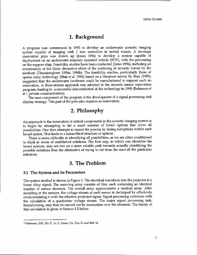
The system studied is shown in Figure 1. The electrical waveform into the projector is a linear chirp signal. The receiving array consists of tiles, each containing an identical number of sensor elements. The overall array approximates a random array. After sampling at the sensors, the voltage stream at each sensor is dechirped by effectively crosscorrelating it with the effective projected signal. Signal processing continues with the calculation of a quadrature voltage stream. The major signal processing task, beamforming, may then be carried out by summation over the elements. The theory of this calculation is given in Section 3.2 below.

i Robinson, D.E., Ho, P., Li, Y., Jones, I.G., Fox, D. and Bell, M.

DSTO-TN-0098

Receiving Array

r = r: Image point-

Target points

Figure 1: The geometry of the imaging system. The acoustic wave emanating from the projector at 0 is scattered from a typical target point T and received at the n th array element located at Rn. The image point P is a typical point at which the image

intensity is to be calculated.

DSTO and its collaborators are working towards a final design for a sonar for imaging suspected mines. A set of parameters typical of what the expected design might be is given below. The central frequency is determined by a balance between the need to achieve high resolution and the need to avoid strong attenuation in the water. (Approximate angular resolution, or beamwidth measured at 3 dB points, is AjL,

where Xc = wavelength at central frequency and L = diameter of array.) The bandwidth is chosen large enough to give the desired range resolution. (Approximate range resolution, specified by the 3 dB beamwidth, is c/2B, where c = speed of sound

and B = bandwidth of rectangular-window chirp. Note that the theoretically required bandwidth Bth comes out to be 0.75 MHz.) The number of elements is chosen to make the distant sidelobe level sufficiently small. The sampling rate is chosen high enough to avoid the need for interpolation when beamforming. The abovementioned set of

parameters is:

central frequency bandwidth (approx.) diameter of array number of elements number of tiles sampling rate number of samples in received chirp

number of voxels

speed of sound effective signal

3.5 MHz 1MHz 430 mm 4000 100 (40 elements per tile) 20 MHz

80xl03

1000x1000x3000 = 3xl09

(1000 for each angle, range 1 m to 4 m at 1 mm steps)

1500 m/s single shaped, linear chirp, interval

3-4 MHz

DSTO-TN-0098

3.2 Beamforming: Theory

The basic equation for the beamforming is: n(r) = ^nEn[L(r,n)/c] (1)

n

(This method of beamforming in the near and very near field has been briefly described by Knudsen 1989.) In Equation (1), n(r) is the in-phase image amplitude at the 'image point' r, which eventually must be combined with the quadrature part to give the image intensity. (Alternatives to the use of the quadrature part, in particular peak detection, are possible.) Also wn is the weight (shading) assigned to the nth

element, while En(t)is the voltage signal at the nth element at time t. L(r,n) is the

round-trip distance from the projector (at the origin) to r (the image point) and back to the nth element (at R„), given by

Z(r,n) = r + |r-R„| (2)

(Figure 1). In Equation (1), £„(•) must be taken to mean the voltage after dechirping. It is

further assumed that a discrete Hubert transform of En(t) is then performed to yield

E n(t), the quadrature part of the voltage, to be stored along with En(t). Furthermore

both functions are then multiplied by the weight wn to yield new stored values

FM = ">Mt) and Fqn(t) = wnEqn(t), (3)

the weighted voltages. To express Equation (1) in a form that shows most clearly the computing problem,

consider the image point to be at the centre (r,) of the ith voxel. Then (1) may be

written as 4xlOJ

(5)

n,-= £FB[* = r(/,»)] i = i,-,3xio9. (4)

Here T(i, n) = L(i, n)/c is the round-trip time, given by

r(/,«) = [Hr,.-R„|]/c = [rl+tf-2rrRm+tiT]/c;

while IT,. =n(r.).

3.3 Computation Times

3.3.1 Dechirping; the Quadrature Part

Before performing beamforming proper, some preliminary procedures must be carried out: dechirping of each voltage stream, calculation of the quadrature part of each stream (Section 3.2) and the minor procedure of weighting the voltages (Eqn 3). As discussed in Blair (1997, Section 5.4.2), the number of multiply or add (MAD)

DSTO-TN-0098

operations required to perform all of the above is about 10x4000x(8xl04) xlOg2(8xl04), there being 4000 elements and 8xl04 samples in a stream. This is a very small figure compared to the operations required for the main beamforming (calculated in Section 3.3.2). Hence the time for the preliminary procedures can essentially be ignored in deciding the best signal processing strategy.

3.3.2 Beamforming Proper

From Equation (4), the summations in the calculation of the image amplitudes require a total of 4000x(3xl09) = 1.2xl013 operations: double this to include the quadrature part. In addition, there is the calculation of the address for fetching the voltage to be retrieved: we shall call this calculation 'addressing'. It is essentially the calculation of the round-trip distance, Equation (5). This requires the computation time of several MAD operations for every one add in the summation, since the image point lies in the near field. As shown in Blair (1997), a fifth degree polynomial is a suitable expression for the distance; as a result, addressing plus quadrature causes the above figure of 1.2xl013 to expand to 9x(1.2xl013) operations (Blair 1997, Sections 2.4,4.5.2).

Consider a hypothetical '1 Gflops' computer, taken here to mean a computer that performs 109 operations per second, where an 'operation' is deemed to include any associated fetch and store action. For a slightly more general computer in which the add and the multiply operation take different times, the average speed, v Gflops, of a computer during a long calculation depends on the type of calculation. More complex architectures are discussed briefly in Section 8. Note that in this report the term Gflops refers to operations, whether they be floating point or integer operations. A consequence is that a choice of integer arithmetic for the beamforming calculation would normally make the speed of '1 Gflops' easier to achieve.

Based on the 9x(1.2xl013) operations quoted above, a 1 Gflops computer would require T2 = 9Ti = 1.1 *105 seconds = 30 hours to produce the image, unacceptably long for the applications in mind. Further overheads are required by a practical computer to account for the lack of ideal matching between the algorithm and the computer, and also to allow for such items as the display. These require a further 'factor of safety' which we will take to be 2. The computation time then becomes 60 hours.

4. Broad Approaches

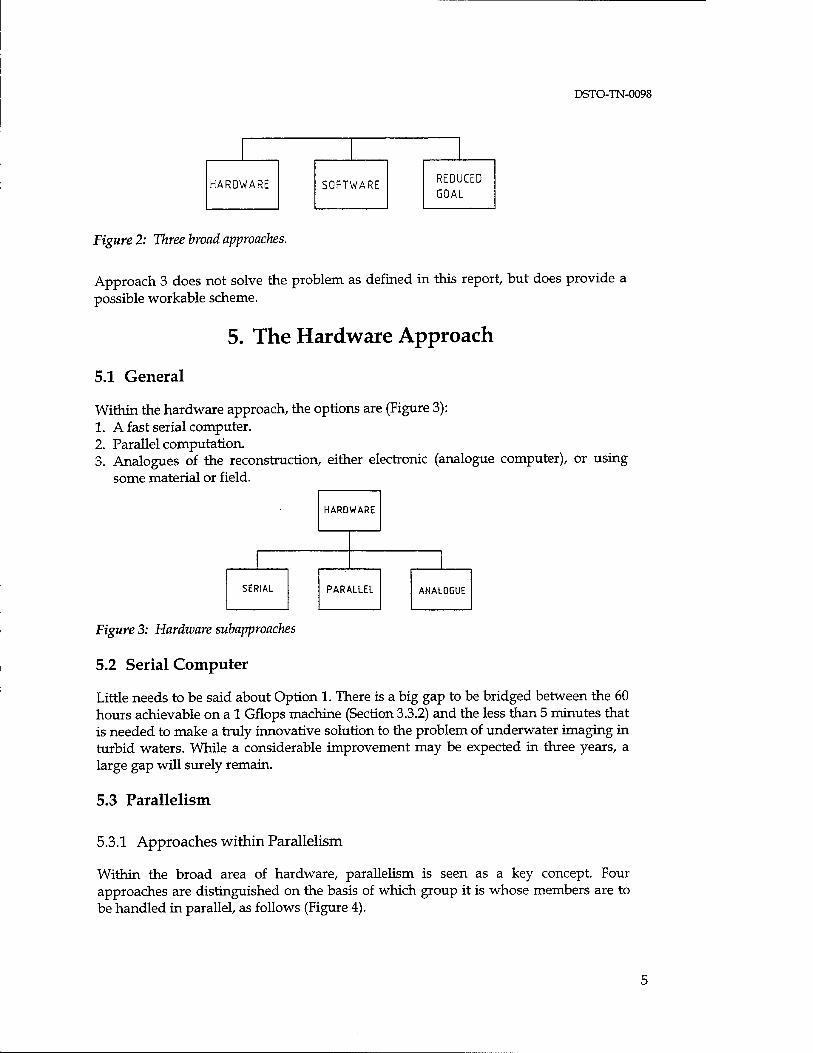
Three broad approaches were identified (Figure 2): 1. Solution by appropriate hardware. 2. Solution by appropriate software to reduce the number of operations. 3. Define a reduced goal as being what is acceptable in the end product.

DSTO-TN-0098

HARDWARE SOFTWARE REDUCED

GOAL

Figure 2: Three broad approaches.

Approach 3 does not solve the problem as defined in this report, but does provide a possible workable scheme.

5. The Hardware Approach

5.1 General

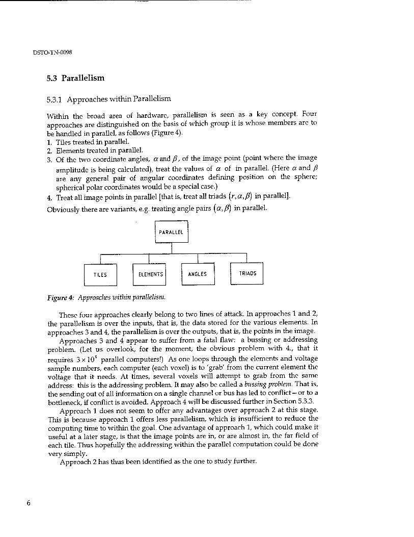
Within the hardware approach, the options are (Figure 3): 1. A fast serial computer. 2. Parallel computation. 3. Analogues of the reconstruction, either electronic (analogue computer), or using

some material or field.

HARDWARE

SERIAL PARALLEL ANALOGUE

Figure 3: Hardware subapproaches

5.2 Serial Computer

Little needs to be said about Option 1. There is a big gap to be bridged between the 60 hours achievable on a 1 Gflops machine (Section 3.3.2) and the less than 5 minutes that is needed to make a truly innovative solution to the problem of underwater imaging in turbid waters. While a considerable improvement may be expected in three years, a large gap will surely remain.

5.3 Parallelism

5.3.1 Approaches within Parallelism

Within the broad area of hardware, parallelism is seen as a key concept. Four approaches are distinguished on the basis of which group it is whose members are to be handled in parallel, as follows (Figure 4).

DSTO-TN-0098

5.3 Parallelism

5.3.1 Approaches within Parallelism

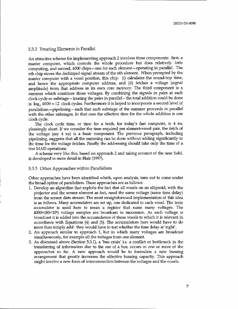
Within the broad area of hardware, parallelism is seen as a key concept. Four approaches are distinguished on the basis of which group it is whose members are to be handled in parallel, as follows (Figure 4). 1. Tiles treated in parallel. 2. Elements treated in parallel. 3. Of the two coordinate angles, a and ß, of the image point (point where the image

amplitude is being calculated), treat the values of a of in parallel. (Here a and ß axe any general pair of angular coordinates defining position on the sphere; spherical polar coordinates would be a special case.)

4. Treat all image points in parallel [that is, treat all triads (r, a,ß) in parallel].

Obviously there are variants, e.g. treating angle pairs (or,/?) in parallel.

PARALLEL

|

TILES ELEMENTS ANGLES TRIADS

Figure 4: Approaches within parallelism.

These four approaches clearly belong to two lines of attack. In approaches 1 and 2, the parallelism is over the inputs, that is, the data stored for the various elements. In approaches 3 and 4, the parallelism is over the outputs, that is, the points in the image.

Approaches 3 and 4 appear to suffer from a fatal flaw: a bussing or addressing problem. (Let us overlook, for the moment, the obvious problem with 4., that it requires 3 x 109 parallel computers!) As one loops through the elements and voltage sample numbers, each computer (each voxel) is to 'grab' from the current element the voltage that it needs. At times, several voxels will attempt to grab from the same address: this is the addressing problem. It may also be called a bussing problem. That is, the sending out of all information on a single channel or bus has led to conflict—or to a bottleneck, if conflict is avoided. Approach 4 will be discussed further in Section 5.3.3.

Approach 1 does not seem to offer any advantages over approach 2 at this stage. This is because approach 1 offers less parallelism, which is insufficient to reduce the computing time to within the goal. One advantage of approach 1, which could make it useful at a later stage, is that the image points are in, or are almost in, the far field of each tile. Thus hopefully the addressing within the parallel computation could be done very simply.

Approach 2 has thus been identified as the one to study further.

DSTO-TN-0098

5.3.2 Treating Elements in Parallel

An attractive scheme for implementing approach 2 involves three components: first, a master computer, which controls the whole procedure but does relatively little computing, and second, 4000 chips-one for each element-operating in parallel. The nth chip stores the dechirped signal stream of the nth element. When prompted by the master computer with a voxel position, this chip: (i) calculates the round-trip time, and hence the appropriate computer address, and (ii) fetches a voltage (signal amplitude) from that address in its own core memory. The third component is a summer which combines those voltages. By combining the signals in pairs at each clock cycle or substage—treating the pairs in parallel—the total addition could be done in log2 4000 = 12 clock cycles. Furthermore it is hoped to incorporate a second level of parallelism—pipelining—such that each substage of the summer proceeds in parallel with the other substages. In that case the effective time for the whole addition is one clock cycle.

The clock cycle time, or time for a fetch, for today's fast computer, is 4 ns, pleasingly short. If we consider the time required per element-voxel pair, the fetch of the voltage (say 4 ns) is a basic component. The previous paragraph, including pipelining, suggests that all the summing can be done without adding significantly to the time for the voltage fetches. Finally the addressing should take only the time of a few MAD operations.

A scheme very like this, based on approach 2 and taking account of the near field, is developed in more detail in Blair (1997).

5.3.3 Other Approaches within Parallelism

Other approaches have been identified which, upon analysis, turn out to come under the broad option of parallelism. These approaches are as follows: 1. Develop an algorithm that exploits the fact that all voxels on an ellipsoid, with the

projector and the sensor element as foci, need the same voltage (same time delay) from the sensor data stream. The most straightforward implementation of this idea is as follows. Many accumulators are set up, one dedicated to each voxel. The term accumulator is used here to mean a register that sums many voltages. The 4000x(80*103) voltage samples are broadcast in succession. As each voltage is broadcast it is added into the accumulators of those voxels to which it is relevant in accordance with Equations (4) and (5). The accumulators here would have to do more than simply add: they would have to test whether the time delay is 'right'.

2. An approach similar to approach 1, but in which many voltages are broadcast simultaneously, for example all the voltages from one element.

3. As discussed above (Section 5.3.1), a 'bus crisis' i.e. a conflict or bottleneck in the transferring of information due to the use of a bus, occurs in one or more of the approaches so far. A new approach would be to formulate a new bussing arrangement that greatly increases the effective bussing capacity. This approach might involve a new form of interconnection between the voltages and the voxels.

DSTO-TN-0098

We now discuss approaches 1 and 2 in more detail. First, the statement of approach 1 is vague as it stands, since it is not clear how the delay time is to be known to the accumulator or checked for 'rightness'. In one implementation, all accumulators and the central computer would be kept in synchronisation with a clock, so that each accumulator 'knows' when each data item will be broadcast. At the start, or while waiting between relevant data items, each accumulator calculates which delay time, and which (nearest) sample number, is relevant to it in respect of each element. It 'grabs' the data item emanating at the appropriate time.

Second, approach 1 seems to face a major difficulty, for it requires 3><109

accumulators, one for each voxel; this is a vast number of accumulators. Moreover, each accumulator is not all that simple for, besides undertaking summation, these accumulators must also calculate the time delays.

Third, consider approach 2. Whatever bussing problem there is in approach 1, the bussing problem in approach 2 is far worse. In the extreme case where all the voltages from all elements are broadcast at once, the system is massively parallel at both voxels and sensors, and hence bus overloading is highly likely.

We now see that approach 1, as it has been developed, is identical to the developed form of approach 4 of Section 5.3.1.

A certain variant of approach 1, and perhaps of the other approaches, must be warned against. The variant involves, for each combination of element and voltage sample number, ascertaining the voxels for which that combination will be used in the sum. This variant requires 27 times as many calculations of round trip time as does approach 1 or the method of Section 5.3. This is so because the variant involves, for each element and sample number combination, the calculation, for each angle pair (a,ß), of the range r at which the round trip time agrees exactly with the time of the

sample voltage. A voxel at (a,ß) centred at r, or in a certain small interval

surrounding r, would 'accept' the corresponding voltage into its summation. In this variant the number of ranges calculated (each calculation being the equivalent of a round trip time calculation) would be, from the data of Section 3.1,

106x(4xl03)x(80xl03) = 3.2xl014. On the other hand, in approach 2 of Section 5.3.1, calculations of path lengths would replace calculations of ranges. The number of such calculations would be

(3xl09)x4000 = 1.2x1013, which is less by a factor of 27, as previously stated. Approach 2 of Section 5.3.1 is therefore preferred.

Note that the argument shows that the 'certain small interval' of range surrounding r is smaller than the voxel size (1 mm) by a factor 27. For a given combination of a pair of angles and an element, only one voltage in 27 makes any contribution.

DSTO-TN-0098

5.4 Analogues of the Reconstruction

Methods using analogues include the following. 1. Backpropagation in water would reproduce the image as a pressure field. Water

'solves the problem easily'. But problems are: first, how the user is to see the image, and second, how to obtain hard copy, e.g. a photograph.

2. Develop an analogue of water in a computer and/ or electronics. It appears that such an analogue is more feasible via a digital than via an analogue computer.

3. The alternative to sound in water is light in air. If the original ensonification of the object by the acoustic imaging system is imagined as a pulse of sound, travelling away from the sonar as a spherical wave, it sweeps across the underwater object to be imaged, ensonifying slices of space in succession. If the received signal could be replayed as a coherent optical source at a set of scaled locations corresponding to the elements of the sparse array, the light would similarly sweep out and reconstruct the volume reflectance of the target, slice by slice, the slice being reproduced at the same distance as the original slice, but scaled. Conceptually a screen moving away from the light source would have projected on it at all times the image of the current slice. The reproduction would be somewhat like viewing the object through a moving slit.

6. The Software Approach: Reducing the Number of Operations

6.1 Background

The equation for beamforming is Equation (4) given in Section 3.2. This equation

implies 2 x (1.2 x 1013) additions (to include the quadrature terms), after the time Thas

been calculated for 1.2 x 1013 combinations (i, n). If the whole image is to have data in it, there is a minimum of 3><109 steps to fill the voxels. The number of operations for beamforming surely cannot be made less than this. If the computing capacity is 1 Gflops (109 operations per second), it will take 3 seconds just to refresh the voxels.

New hardware and new software often go hand in hand. In this report, we take the distinguishing feature of a 'software solution' to be that it reduces the number of operations to be performed.

6.2 Approaches

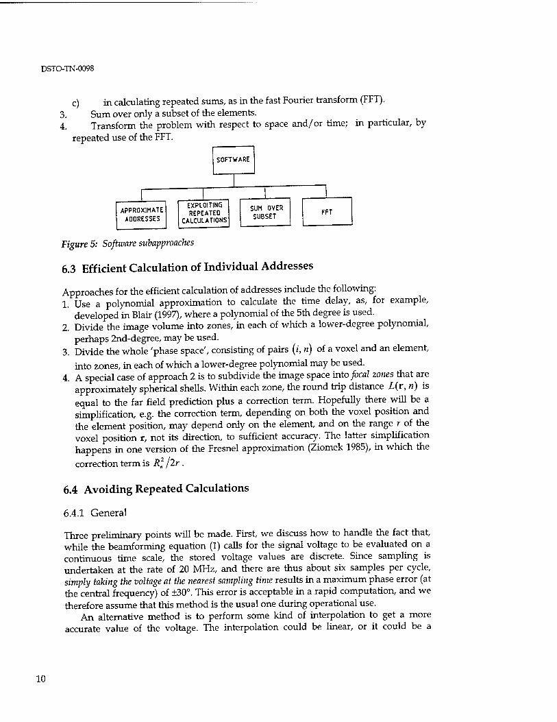
The alternative software approaches are (Figure 5): 1. Calculate each address more efficiently, by replacing the square root with

something more quickly calculable. 2. Avoid repeating calculations, either:

a) in calculating the same or similar addresses, b) in calculating, plus fetching from, the same address, or

DSTO-TN-0098

C) in calculating repeated sums, as in the fast Fourier transform (FFT). 3. Sum over only a subset of the elements. 4. Transform the problem with respect to space and/or time; in particular, by

repeated use of the FFT.

SOFTWARE

APPROXIMATE AOORESSES

EXPLOITING REPEATED

CALCULATIONS

SUM OVER SUBSET

ZL FFT

Figure 5: Software subapproaches

6.3 Efficient Calculation of Individual Addresses

Approaches for the efficient calculation of addresses include the following: 1. Use a polynomial approximation to calculate the time delay, as, for example,

developed in Blair (1997), where a polynomial of the 5th degree is used. 2. Divide the image volume into zones, in each of which a lower-degree polynomial,

perhaps 2nd-degree, may be used. 3. Divide the whole 'phase space', consisting of pairs (i, n) of a voxel and an element,

into zones, in each of which a lower-degree polynomial may be used. 4. A special case of approach 2 is to subdivide the image space into focal zones that are

approximately spherical shells. Within each zone, the round trip distance L(r, n) is equal to the far field prediction plus a correction term. Hopefully there will be a simplification, e.g. the correction term, depending on both the voxel position and the element position, may depend only on the element, and on the range r of the voxel position r, not its direction, to sufficient accuracy. The latter simplification happens in one version of the Fresnel approximation (Ziomek 1985), in which the

correction term is R] jlr .

6.4 Avoiding Repeated Calculations

6.4.1 General

Three preliminary points will be made. First, we discuss how to handle the fact that, while the beamforming equation (1) calls for the signal voltage to be evaluated on a continuous time scale, the stored voltage values are discrete. Since sampling is undertaken at the rate of 20 MHz, and there are thus about six samples per cycle, simply taking the voltage at the nearest sampling time results in a maximum phase error (at the central frequency) of ±30°. This error is acceptable in a rapid computation, and we therefore assume that this method is the usual one during operational use.

An alternative method is to perform some kind of interpolation to get a more accurate value of the voltage. The interpolation could be linear, or it could be a

10

DSTO-TN-0098

Fourier-based procedure. In the Fourier procedure, one pads the signal in the frequency domain with zeros and then performs an inverse transform. A possible concern is that the very noisy raw signal that may be obtained if one-bit quantisation is used may invalidate the whole interpolation procedure or cause it to constitute no advance over the use of the nearest sampling time. It would seem that this threat could be removed during the Fourier procedure by retaining only those frequency components that lie in the signal's known bandwidth. Presumably it is best to remove such components at the time of dechirping, prior to any beamforming.

We have been unable to estimate how noisy the data is from an individual sensor element after dechirping has been performed. More research in this area is needed. We shall proceed on the assumption that, when interpolation or extrapolation procedures are carried out, the noise is small enough to render these procedures valid.

As a second preliminary point, we distinguish between relative and absolute addresses of signal voltages. These terms refer to a metaphor (which is reality in many hardware implementations) in which the voltages for one element are stored sequentially in a block, in the order of the times at which the sensor element took that reading. And likewise for each other element, the voltages being stored with a constant address offset from those of the first element. Equality of two relative addresses, i.e. addresses of two voltages relative to the beginning of their respective blocks, implies that the round-trip times are the same. (Recording begins for all elements at the same time.) There is no implication that the elements are the same. Equality of two absolute addresses implies that the round-trip times are the same and that the two elements are actually the same element. These concepts become relevant when we consider two voxels. If, for the same element, the two voxels call for the voltage from the same voltage sample number (same round-trip time) to be used in the summation, the two voxels are calling for a voltage from the same absolute address. But if, for two different elements, two voxels call for the same voltage sample number, the voxels are merely calling on the same relative address. Clearly the 'absolute' case leads to a potential for savings in computing time since, if several absolute addresses are known to be equal, that address need only be calculated once. In the case of 'relative' equality, one could still gain appreciable savings in the number of computing operations, for if many known combinations (i, n) of a voxel and an element are known to require the same relative address, it again suffices to calculate that address once. Then each absolute address is obtained by a single further addition.

Third, in the sections below, 'hard' and 'soft' equality of two round-trip distances will be defined. While each of these could be combined with each of the suboptions (in option 2 in Section 6.2) of avoiding repeated calculations, to keep the discussion within bounds only certain combinations are discussed below, being the ones that seem most promising.

11

DSTO-TN-0098

6.4.2 Repetition of Relative Address

This section deals with approach 2a in Section 6.2.

6.4.2.2 Definition and Potential To avoid a repeated calculation of the same relative address, we must look for a set P of pairs (i, n) of a voxel and an element, such that the resulting round-trip distances

L(i, n) are all equal. There may be many sets P. For significant savings in operations,

the sets P should together cover most of the full set of pairs (i, n). From Equation (5), the savings-i.e. the savings from not having to recalculate the

relative address-per addition in the summation (4), are the elimination of the square root extraction plus the small number of multiply-or-add operations (MADs) required in calculating the path length L, perhaps the equivalent in all of 10 MADs. Retained are the add in the summation, the add in getting the absolute address from L and a fetch of the voltage. Ignoring the fetch in accordance with Section 3.3.2, we have 2 MADs retained. The savings therefore involve a reduction in the number of MADs from 12 to 2. On these figures, and assuming that every voxel-element pair can be incorporated in some set P containing (say) 15 or more other pairs, the factor by which the number of operations is reduced is 12/2, or 6. This is an optimistic estimate and represents the potential savings. Hence the savings available by this software approach alone are not great. These savings might well be wiped out by the overheads involved in organising the multiple use of the one round-trip distance.

The effective time for some or all of the retained operations (two adds and a fetch) might be vastly reduced by suitable parallel computing, to yield a much greater time reduction factor; this would be a combined hardware/software solution.

6.4.2.2 Use of Exact Travel Time Equality We first deal with the case in which the equality of round-trip distances is construed to be exact.

A way in which such exact equalities occur is as follows. Consider the case where the array is used passively and the elements are laid out in a repeating pattern, say a square array. Then the centres of the voxels could be chosen to follow the same geometrical pattern, but in planes parallel to the plane of the array. If the voxel spacing also is the same as, or a submultiple of, the array spacing, then there is a symmetry that makes many path lengths equal.

However, when we move to a two-way system (as the operational system would be), the available symmetries are much reduced, and hence so also are the number of equalities, or repetitions that might be avoided. Changing to a random array also makes repetition much less common. It therefore seems unlikely that practical use can be made of exact equalities.

6.4.2.3 Use of Inexact Equality It may also be possible to use round-trip distances that are only approximately equal. To assist the discussion we define a 'hard' and soft' equality. Two round-trip distances

12

DSTO-TN-0098

!,(/,,«,) and L(i2,n2) are said to be equal in the hard sense if, when scaled and

rounded, they yield the same relative address. A 'soft' equality (precise definition given later) is one where the difference in travel time is larger than in the case of a 'hard' equality.

In the 'soft' case, the acquiring of the common part of the distance is only the first step, since a correction to the voltage still needs to be computed for each voxel-element pair. This implies a considerable overhead. When using the relative address approach, because that approach offers only modest savings, it seems wise to combine it with a method offering considerable savings at the point of calculating the distance with sufficient precision. This means using exact or hard, rather than soft, equality. This recommendation is followed below.

The above conclusions may have to modified where some special relationship exists. An example might be where the voxels are close together or the elements are close together.

6.4.3 Repetition of Absolute Address

This section deals with approach 2b in Section 6.2.

6.4.3.1 Definition and Potential To avoid a repeated calculation of the same absolute address, we must look for a single element n and a set / of voxels i, such that the resulting round-trip distances L(i, n)

axe all equal in some sense. Let Q be the set of resulting pairs. There may be many sets Q. For significant savings in operations, the sets Q should together cover most of the full set of pairs (z, n).

As in Section 6.4.2.1, the savings, per addition in the summation (4), are the elimination of a square root extraction plus a small number of MAD operations, perhaps the equivalent in all of 10 MADs. Retained is just the add in the summation (and no longer the add in getting the absolute address), and hence 1 MAD. On these figures, and assuming that every voxel-element pair can be incorporated in some set Q, the factor by which the number of operations is reduced is now (10 + l)/l = 11. Again this factor represents the potential savings. Hence the savings available by this software approach alone are somewhat improved, compared to the 'relative address' approach (Section 6.4.2.1). Furthermore, the overheads involved in organising the multiple use of the one round-trip distance are improved, since the program would work with only one element at a time (the relevant paths all end on the same element).

Again the effective time for the retained operation—the add in the summation— might be greatly reduced by parallel computing (a combined hardware/software solution).

The advantages of the absolute address approach over the relative approach have just been described. The advantage of the relative approach is that, given a particular round-trip distance, use is made of its being shared by many more entities, i.e. voxel- element pairs. (In the absolute approach, sharing is with voxels, the element remaining fixed. Of course, in the comparison of absolute with relative, the same concept of 'equality', for example 'hard', must be used throughout.)

13

DSTO-TN-0098

6.4.3.2 Quantitative Potential for Matches in the Case of Hard Equality We consider first the equality of absolute addresses. In particular we calculate, for a

typical element and voxel, how many other voxels have the same round-trip time in the hard sense. We assume a polar grid of voxels, of spacing 1 mm in range and 1 mrad in each of two directions. For a given element, the surface of image points (same as voxels but forming a continuum) having constant round-trip distance is an ellipsoid. The ellipsoid through the chosen voxel (the 'first' voxel) is always inclined at an angle that is small to the spherical grid surfaces that are spaced at vr = 1 mm, where vr is the

voxel size in range. Thus, in each solid angle of 1 (mrad)2, the ellipsoid is within vr /2 of some second voxel. If its radial distance from that second voxel is sufficiently small, hard equality will apply between the round-trip times for the two voxels. We denote by p the probability that, in a randomly chosen solid angle of 1 (mrad)2, there is a voxel for which hard equality with the first voxel obtains.

To sufficient accuracy, the round-trip time is (spherical approximation) T = L/c*2r/c.

This equation 'translates' between times T and ranges r via a factor c/2. As stated, in each solid angle of 1 (mrad)2, the ellipsoid is within vr/2 of some second voxel. The

'hard' criterion is that the ellipsoid lies within the 'distance' TJ2 of that voxel, in terms of time, where Ts is the sampling interval; or equivalently, within

(C/2)(TJ2) =CTJ4 of that voxel in distance. The probability p of hard equality is

then the ratio of the two distances:

P = {cTj4)/{vr/2) = cTj2vr. (6)

Inserting Ts = 0.05 x 10'6 s and vr = 1 mm from Section 3.1, we obtain the probability

/> = 0.0375. This means that, given any element and any voxel, there are

103 xl03x 0.0375 = 3.75 xlO4

voxels sharing the same round-trip time with the first voxel in the hard sense. There is no shortage of 'matching' voxels, even in this 'hard, absolute' case. The problem is to find them efficiently loithout actually calculating all tlie distances (which would defeat the whole purpose).

The corresponding result for relative addresses follows immediately. Given any voxel-element pair, the number of pairs sharing the same round-trip time in the hard

sense is 4000 times the above figure of 3.75 x 104, or 1.5 x 108, the 4000 being the number of elements.

The result (6) can be connected to other results. First, from Section 3.1, the probability may be written as

P = BthTs,

where £„, is the bandwidth theoretically required to yield resolution vr. In Section 5.3.3, a certain ratio was found to have the value 27. Retracing the argument for the general case (symbols, not numbers), we find that ratio to be 2vr /cTs. This is the reciprocal of (6); in particular, we have 1/0.0375 « 27. This is no coincidence, since

14

DSTO-TN-0098

Section 5.3.3 deals with two step sizes in range: vr and cTjl (or equivalent^, half of

each of these), related by this very ratio.

6.4.4 Repetition of Summations

This section deals with approach 2c of Section 6.2.

6.4.4.2 Definition and Potential The approach is to find those operations that involve common sums and store these sums for multiple later use.

To avoid repeating sums, we must look for a set I of voxels and a set N of elements such that, for each element n in N, the resulting round-trip distances L(i, n)

for all voxels i in 7 are all equal. Let R be the Cartesian product of I and N, that is, the set of all such pairs (i, n). There may be many sets R. For significant savings in

operations, the sets R should together cover most of the full set of pairs (i, n) . We now turn to the savings in operations. Assuming that every voxel-element pair

can be incorporated in some set R such that N contains many elements, the factor by which the number of operations is reduced is the number of voxels in I (assumed to be a constant). This number could be very large. Thus summation avoidance gives a potential reduction much greater than for relative or absolute address avoidance. However such a large reduction hinges on the overheads being kept low. The overheads of concern are of two types: first, the extrapolation of the voltages associated with soft equality, and second, the determination, with little or no calculation, of what voxels and elements to group together.

6.4.4.2 Soft Equality Defined Repetition of summations necessarily involves moving away from hard equality, since a number of elements are involved in any repeated sum. We turn to 'soff equality, which requires a slight modification of the discussion of Section 6.4.3.2. In particular, a further overhead is introduced, and it is likely to be the dominant overhead. That overhead is the need to extrapolate in order to obtain one voltage from another.

Equality in the soft sense is based on the idea that, for a given element, the voltage, which is essentially the summand in Equation (1), for image points r in the neighbourhood of some fixed point r0 can, within some limited accuracy, be predicted

by extrapolation from the dechirped voltage £„[l(r0, n)/c] evaluated for image point

r . Given two image points and the associated round-trip distances to the same

element, the two round-trip distances are equal in the soft sense if the voltage at one image point can be predicted from the voltage at the other.

To make the definition more precise, two issues need to be considered. First, the mode of extrapolation. Because of the limited bandwidth, for any t and t0 sufficiently close together, we have for the analytic dechirped signal the following extrapolation formula:

E.(?)=En(t0)GX^j2xfe(t-t0)] (7)

15

DSTO-TN-0098

where fc is the central frequency of the chirp. In a zeroth order approximation of the

far-field type, we have

L(r,n)-L(r0,n) = 2(r-r0) (8)

where the two rs on the right-hand side are magnitudes only. By substituting t = I(r, n)/c and t0 = L(r0,n)/c in (7) and using (8), we obtain

En[L(r, n)/c] = En[L{r0,n)/c] QxV[j4^fc{r -r0)} (9)

as the extrapolation formula. (Note the "zeroth order" above. We do not rule out the possibility that further terms beyond the zero-order term need to be used in Eqn 8 to obtain a sufficiently accurate extrapolation formula.) The caution about extrapolation in Section 6.4.1 applies here.

The second issue concerns the acceptable accuracy. The dechirped voltage signal contains frequency components out to f = fc±B/2, where B is the bandwidth. (Here a rectangular envelope of the effective chirp spectrum is assumed.) Due to the

use of (7), a frequency component acquires a phase error as \t-t0\ increases. Due to

the use of (8), in general it acquires a further phase error. We suggest the following criterion: When the maximum error (due to the two effects combined) reaches ±90° (signifying that the correlation between the true and approximate components has reached zero), soft equality is said to no longer hold between the path length via the image point r and the path length via r0, both paths being round trips terminating at

the element n. There may be an acceptable image formation with extensive use of the 'soft'

inequality.

6.5 Subset of Elements

Possibly an approximation to Equation (1) can be developed that does not use all of the 4 x 103 elements. It must be recognised that something is then lost: at the least, the clutter (distant sidelobe level) is increased. A possible way of dealing with the loss is to form the image using the subset of the elements, pick out the most interesting region in the image, and finally recalculate the image in that region using all elements.

A first way of choosing the subset would be to drop the elements that are less important in forming the image, if indeed any elements can be so identified. It may be argued that such a dropping effectively occurs whenever an array is shaded (apodised). For one way of shading the array is, not to assign reduced weights nearer the edges, but to drop altogether from the sum some elements nearer the edges. (Of course there is a penalty in resolution here, offset by an improvement in the near sidelobes.) Thus the improbable-sounding 'first way' is not entirely without merit.

A second choice of the subset of elements is to make the array more sparse by removing elements at random, uniformly thinning the array. This implies no reduction in the effective aperture and therefore no loss in resolution. This basic idea is taken up again in Section 7 as one of the methods of providing more information for the choice of a subvolume for which the image is to be computed 'precisely'.

16

DSTO-TN-0098

6.6 Fast Fourier Transform

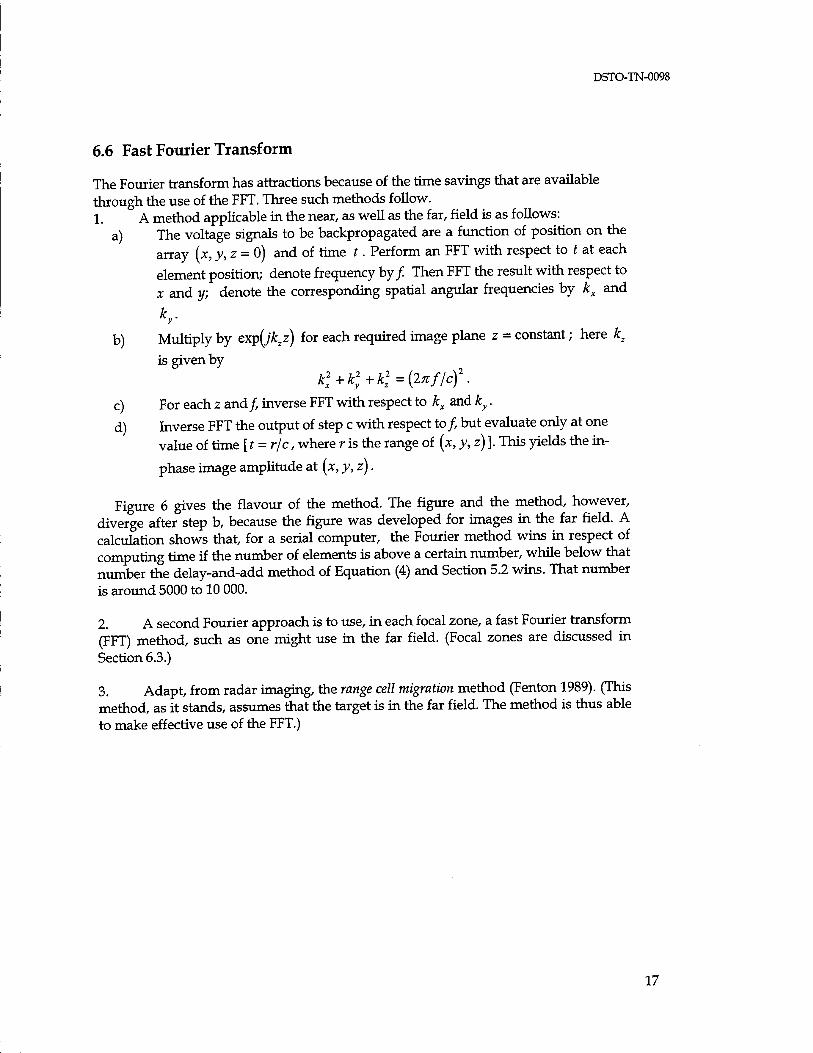
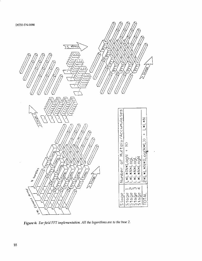
The Fourier transform has attractions because of the time savings that are available through the use of the FFT. Three such methods follow. 1. A method applicable in the near, as well as the far, field is as follows:

a) The voltage signals to be backpropagated are a function of position on the array (x, y, z = 0) and of time t. Perform an FFT with respect to t at each

element position; denote frequency by/ Then FFT the result with respect to x and y; denote the corresponding spatial angular frequencies by kx and

V b) Multiply by exp(jkzz) for each required image plane z = constant; here k2

is given by k2

x+k2y+k2

2={2xfjc)2.

c) For each z and/, inverse FFT with respect to kx and ky.

d) Inverse FFT the output of step c with respect to /, but evaluate only at one value of time [ t = r/c, where r is the range of (x, y, z) ]. This yields the in-

phase image amplitude at (x, y, z).

Figure 6 gives the flavour of the method. The figure and the method, however, diverge after step b, because the figure was developed for images in the far field. A calculation shows that, for a serial computer, the Fourier method wins in respect of computing time if the number of elements is above a certain number, while below that number the delay-and-add method of Equation (4) and Section 5.2 wins. That number is around 5000 to 10 000.

2. A second Fourier approach is to use, in each focal zone, a fast Fourier transform (FFT) method, such as one might use in the far field. (Focal zones are discussed in Section 6.3.)

3. Adapt, from radar imaging, the range cell migration method (Fenton 1989). (This method, as it stands, assumes that the target is in the far field. The method is thus able to make effective use of the FFT.)

17

DSTO-TN-0098

U1 Qj

-P d 2 15 Z u

* _J * _J

u <r + \ s\ >, /-N —' /-\ 1 (_L 2 * -P Z — + ^-Sf -S rf\ U) X 21 n

(-T) 1 1 j£- i Ci_ nOCDOi \^ o ■ o o o *

* _J_J_J z. i. ~Z? X ^ ^

6zzz x

Q; _j O JTS ^\ /T\ y*«. * € _J_J_I_I _J "5 ?K /N /rC ^ * z _J_J_J_1 0J

^ajn^r

OJ Qj CU CU Cu _l O) OCDCTCD <E a ÖÖÖÖ I—

o-> j_> _!_> _(_> -_> □ C/) <y) oo oo oo 1—

Figure 6: Far field FFT implementation. All the logarithms are to tlie base 2.

18

DSTO-TN-0098

7. The Reduced Goal Approach

7.1 Reduction of the Problem

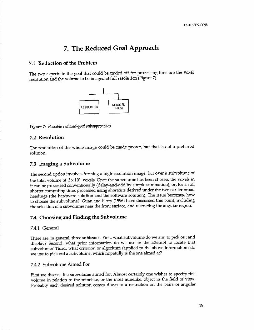
The two aspects in the goal that could be traded off for processing time are the voxel resolution and the volume to be imaged at full resolution (Figure 7).

RESOLUTION REDUCED

IMAGE

Figure 7: Possible reduced-goal subapproaches

7.2 Resolution

The resolution of the whole image could be made poorer, but that is not a preferred solution.

7.3 Imaging a Subvolume

The second option involves forming a high-resolution image, but over a subvolume of the total volume of 3 x 109 voxels. Once the subvolume has been chosen, the voxels in it can be processed conventionally (delay-and-add by simple summation), or, for a still shorter computing time, processed using shortcuts derived under the two earlier broad headings (the hardware solution and the software solution). The issue becomes, how to choose the subvolume? Guan and Perry (1996) have discussed this point, including the selection of a subvolume near the front surface, and restricting the angular region.

7.4 Choosing and Finding the Subvolume

7.4.1 General

There are, in general, three subissues. First, what subvolume do we aim to pick out and display? Second, what prior information do we use in the attempt to locate that subvolume? Third, what criterion or algorithm (applied to the above information) do we use to pick out a subvolume, which hopefully is the one aimed at?

7.4.2 Subvolume Aimed For

First we discuss the subvolume aimed for. Almost certainly one wishes to specify this volume in relation to the minelike, or the most minelike, object in the field of view. Probably each desired solution comes down to a restriction on the pairs of angular

19

DSTO-TN-0098

coordinates, and a specification of an interval of ranges at each allowed pair of angular coordinates.

Regarding the interval of range, what comes immediately to mind is to select an interval near the front surface of the minelike object. However, one may wish to look elsewhere. For example, where there is a thick plastic insert, one may wish to, and be able to, look for the back surface of the insert, to determine the thickness, which may be useful in mine identification. Note that we expect reflections from the second, or back, surface to be detectable only when the impedance of the material is close to that of seawater (or when the thickness is less than 1/4 wavelength-but this case is in fact not relevant since the second surface would be within the same voxel).

A further consideration is the thickness of the slice (subvolume) in the range direction, given that the central range of the slice is at (or near) the surface of the object. It is desirable to have the thickness larger rather than smaller, because first, the surface may have considerable projections and depressions, and second, the original estimate of the range to the surface may have been in error.

One desirable aim is to image in all directions (though only over an interval of ranges). This is because first, the mine, at a range of 1-2 m, occupies an area approximately equal to the field of view, and second, one may be wrong in picking out a particular sector as being the sector that has the most significance. Suppose, however, that time considerations force us to restrict imaging to a sector: how should that sector be chosen? It seems that the only answer that can be given is, the sector that, on the basis of prior information, is most likely to be useful in mine identification. This selection is difficult to automate; one criterion could be the sector in which the surface is as different as possible from being a smooth, featureless surface. Since such criteria seem inadequate, we are left with manual selection of the sector on the basis of prior information.

7.4.3 Prior Information

Second, we turn to the question of the prior information to be used. One source of such information is the sending-out of a ping in one direction, or several pings in different directions, to determine the distance to the surface in those directions. Here a separate, additional sonar is envisaged (possibly the relocation sonars common on ROVs). This method gives range information, but not information regarding which sector(s) is most significant.

A second source of information is a coarse, i.e. low-resolution, image that can be generated from the data already stored (ready for processing to yield the high- resolution image). Because it is coarse, the image can be generated in a much shorter time than the full high-resolution image.

A third source is to produce an image from the data already stored, this time at full resolution (and covering the whole field), but allowing increased clutter (noise due to distant sidelobes). This image can be produced in a shortened time by using an array (subset of the elements) that is much sparser than the whole array but that extends across the entire aperture. As the number of elements in the array decreases, the resolution stays the same but the signal-to-noise ratio becomes poorer. Note that an image can be high-resolution or low-resolution (coarse), and may be 'noisy' or Tow-

20

DSTO-TN-0098

noise'. Only in the high-resolution, low-noise case will we say that the image is of 'high quality'. Each of the other three combinations will be called 'low-quality'.

A fourth source of information might be an image from a video camera. Presumably the image is poor or nonexistent since turbidity is forcing the use of the sonar method, but there may be a restricted class of situations where the video image is good enough to give the approximate range of the surface, and also to give the angular regions of most interest. Note that the video image is only two-dimensional; hence, for the range to be deducible, some indication(s) of absolute length must appear on that image.

7.4.4 Finding the Subvolume

Third, we discuss the criterion used in attempting to locate the subvolume. In respect of determining the range to the front surface, three basic methods have been mentioned in Section 7.4.3, of which we shall comment further only on the second. A good criterion is (for each direction) to take the surface to He at that voxel for which the image intensity is greatest. (Very roughly, the image intensity is the return signal. Clearly a correction must be made for spherical spreading and attenuation.) This procedure is expected to fail on occasions, either because there is a fish, or weed, etc. in front of the minelike object, or, more worryingly, because of noise.

It may be that the most common type of failure occurs when isolated voxels (or small groups of voxels) lying away from the front surface are identified as 'surface'. In this case it would be reasonable to reject the isolated voxels and interpolate between the voxels (at neighbouring directions) that cohere strongly with each other. Thus, one method would be to fit a surface, not too strongly curving, so as to agree with as many bright spots in the coarse image as possible.

In respect of attempting to locate the desired angular sector, little can be added to the discussion of Section 7.4.2.

7.4.5 Variants of the Above Methods

First, if the first angular sector identified turns out not to be the one of most interest, one can, in this variant, proceed to select and process a second sector. (Manual selection of the sector again seems best.)

Second, suppose that one is attempting to specify the front surface with sufficient accuracy, but that a cluster of voxels selected initially as part of the surface seems, before or after high-quality processing, not to be part of the surface. Then one can do the following in each direction: find the range (voxel) with the greatest image intensity, but ignoring those ranges that are close to the said false surface.

Third, in the same circumstance, the following is an alternative course of action. One can (for a cluster of adjoining directions) direct the program to fill in that missing part of the surface simply by interpolating from the immediately surrounding portions of the surface.

Fourth, it may happen that, after processing to produce the 'final' high-quality image, the true front surface seems to extend outside the interval of range assumed (because of projections and depressions), as evidenced by the surface reaching the

21

DSTO-TN-0098

boundary of that interval and/ or the surface being partly missing. In that case one can re-process the data, but over a greater interval of range.

Fifth, the high-quality image may be displayed piece-by-piece, as the results become available. Then any decision to abort the present line of processing, and replace it with another, can be made earlier.

7.5 Use of a Low-Resolution Image

As mentioned previously (Section 7.4.3), a method for generating the needed prior information is to process the stored sonar data rapidly to produce a low-quality image. At first sight, it would seem that a low-resolution image could be obtained simply by making the set of the voxels more sparse (compared to the high-quality image) by a factor of 10 in each of the three directions. This would reduce the calculation time (in a serial computer) by a factor of 103.

This method, however, is not without problems. First, it is not satisfactory simply to calculate the high-quality-and hence the high-resolution-image intensity on a sparsened grid. To see this, consider the problem of finding the range of the front surface by finding the voxel with maximum intensity (maximum reflection). On most occasions the method would miss the surface! What is needed is the image averaged over about 10 voxels in the range direction, and similarly in the two angular directions: a truly low-resolution image.

Consider first averaging in the angular directions. A natural way is to reduce the aperture by a factor of 10 in each of the two directions. This leads to a second problem. The array, sparse in the first place, is now reduced from 4000 to 40 elements. The distant sidelobe intensity (assuming the well-known monofrequency formula of 1/N) comes up to 1/40 of the peak intensity, i.e. -16 dB. It seems that a bright reflection away from the current voxel could well swamp the local reflection. When the front surface is perpendicular to the range direction, this effect will not move the surface but will introduce angular clutter, making the identification of the most 'interesting' sector more difficult. When the surface is at (say) 45° to the range direction, it appears that the effect may move the apparent surface by many voxels.

Consider now averaging in the range direction. The 'natural' solution is to reduce the bandwidth by a factor of 10. To do this, one takes the signal at a given element and passes it through a numerical filter; the relevant processing is done most efficiently in the frequency domain. It is not clear whether such filtering leads to an enhancement of the noise relative to the signal. The noise associated with 1-bit quantisation particularly requires attention. Such an enhancement of noise may again cause the apparent surface to be moved considerably in range.

7.6 Imaging All the Front Surf ace: A Method

A method is proposed here for locating the front surface and imaging all of it in a time of perhaps 10 minutes for a serial 1 Gflops computer. The method is put forward as a 'benchmark', so that others working on the problem may compare the performance of their solution with our benchmark.

22

DSTO-TN-0098

It is assumed that a low-resolution image is first produced, with a resolution of 16 mm in all three directions. In successive steps, the resolution is reduced to 8, 4, 2 and then finally 1 mm. But while the 16 mm image has, in each of its discrete directions, many range voxels, in fact 3000/16 of them, the 8 mm and later images are each limited to a 'slice'; each has only four voxels (four discrete ranges) in each of their discrete angular directions. (In this discussion, 'discrete' refers to the direction to the centre of a voxel.)

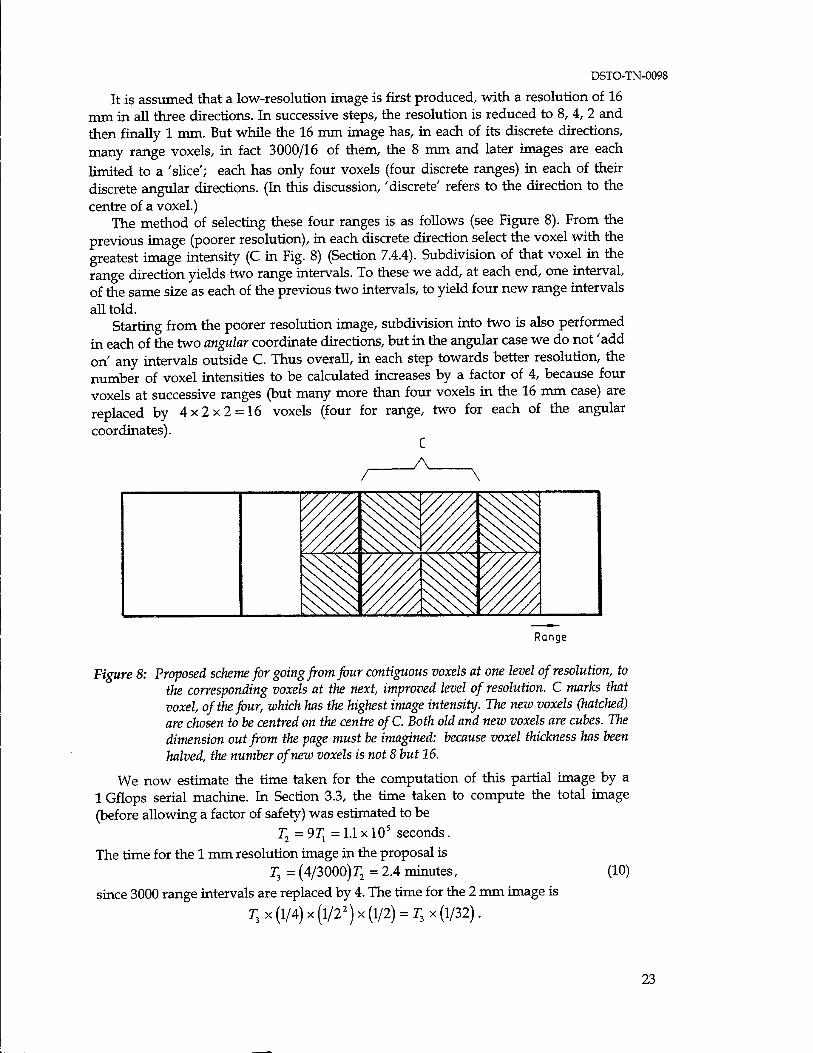
The method of selecting these four ranges is as follows (see Figure 8). From the previous image (poorer resolution), in each discrete direction select the voxel with the greatest image intensity (C in Fig. 8) (Section 7.4.4). Subdivision of that voxel in the range direction yields two range intervals. To these we add, at each end, one interval, of the same size as each of the previous two intervals, to yield four new range intervals all told.

Starting from the poorer resolution image, subdivision into two is also performed in each of the two angular coordinate directions, but in the angular case we do not 'add on' any intervals outside C. Thus overall, in each step towards better resolution, the number of voxel intensities to be calculated increases by a factor of 4, because four voxels at successive ranges (but many more than four voxels in the 16 mm case) are replaced by 4x2x2 = 16 voxels (four for range, two for each of the angular coordinates).

r yv \

Range

Figure 8: Proposed scheme for going from four contiguous voxels at one level of resolution, to the corresponding voxels at the next, improved level of resolution. C marks that voxel, of the four, which has the highest image intensity. The new voxels (hatched) are chosen to be centred on the centre ofC. Both old and new voxels are cubes. The dimension out from the page must be imagined: because voxel thickness has been halved, the number of new voxels is not 8 but 16.

We now estimate the time taken for the computation of this partial image by a 1 Gflops serial machine. In Section 3.3, the time taken to compute the total image (before allowing a factor of safety) was estimated to be

T2 = 9TX = 1.1 x 10* seconds. The time for the 1 mm resolution image in the proposal is

T3 = (4/3000)T2 = 2.4 minutes,

since 3000 range intervals are replaced by 4. The time for the 2 mm image is

T3 x (1/4) x(l/22)x (1/2) = T3x (1/32).

(10)

23

DSTO-TN-0098

Here the 1/4 is for the reduced number of voxels (reduced in the two angular directions only). The remaining factors come from the method described in Section 7.5, putting aside the problems of noise. Thus the 1/22 is for the reduced number of elements. The change in bandwidth implies that the number of samples of the signal may be reduced (Nyquist theorem), leading to the further factor of 1/2. It is readily ascertained that the original low-resolution image is calculated in a time negligible compared to T3. Thus the total time for the sequence of images of increasing resolution

is r3 x [l +1/32 +1/322 +•••] = 2.5 minutes. (11)

To allow for the further operations needed in a practical computer, we again apply a 'factor of safety' of 2; then the time for computing the proposed 1 mm image (including the prior images) is 5 minutes. This time is within the range that would be useful. Modest further reductions may be possible by using a more efficient addressing algorithm (Section 6.3) and by reducing the factor of safety. Larger reductions appear possible via a small degree of parallel computing.

The method has a degree of robustness against small errors in the location of the surface in the four steps (images) leading up to the final image. This is because, upon each subdivision of voxels, not only is the 'brightest' old voxel fully retained, but new voxels are added so that not two, but four, range intervals are imaged. Hence if, in one step, noise causes, not the truly brightest voxel, but the one adjoining it in range, to be selected, a degree of recovery is possible in the next step. Unfortunately the problem of large errors, likely also to occur in practice (Section 7.5), is not dealt with. Perhaps the latter problem can be treated by measures discussed above (Sections 7.4.4, 7.4.5): the fitting of a not-too-curved surface through as many bright points as possible; the option of ignoring an interval of range about the voxel initially but mistakenly selected; and a faculty to manually change the surface.

8. Conclusion

A number of approaches have been described to finding a method of constructing an image from the sparse array that proceeds more quickly than the obvious solution of performing around 9xl.2xl0!3 MAD operations on a serial computer. The three approaches that have been considered can be illustrated by Figure 9. The first, or hardware, approach was to increase the number of gigaflops, v, of the computing machine (by architecture) and this can be represented by moving to the right on the lower axis. Note that increases brought about by parallelism are represented by an increase in v, even though the time taken for a single operation, considered in isolation, may not have been decreased at all. The second, or software, approach was to increase the algorithm efficiency. This is expressed as a, the time taken on a computer as a fraction of the time to calculate the obvious solution (delay-and-add) on a machine ideally matched to the computer code (both machines having the same speed v). Thus, lack of an ideally matched machine may force a from 1 up to 2 for

24

DSTO-TN-0098

60 hr

105

~i 1—i i i

Computer speed Gflops

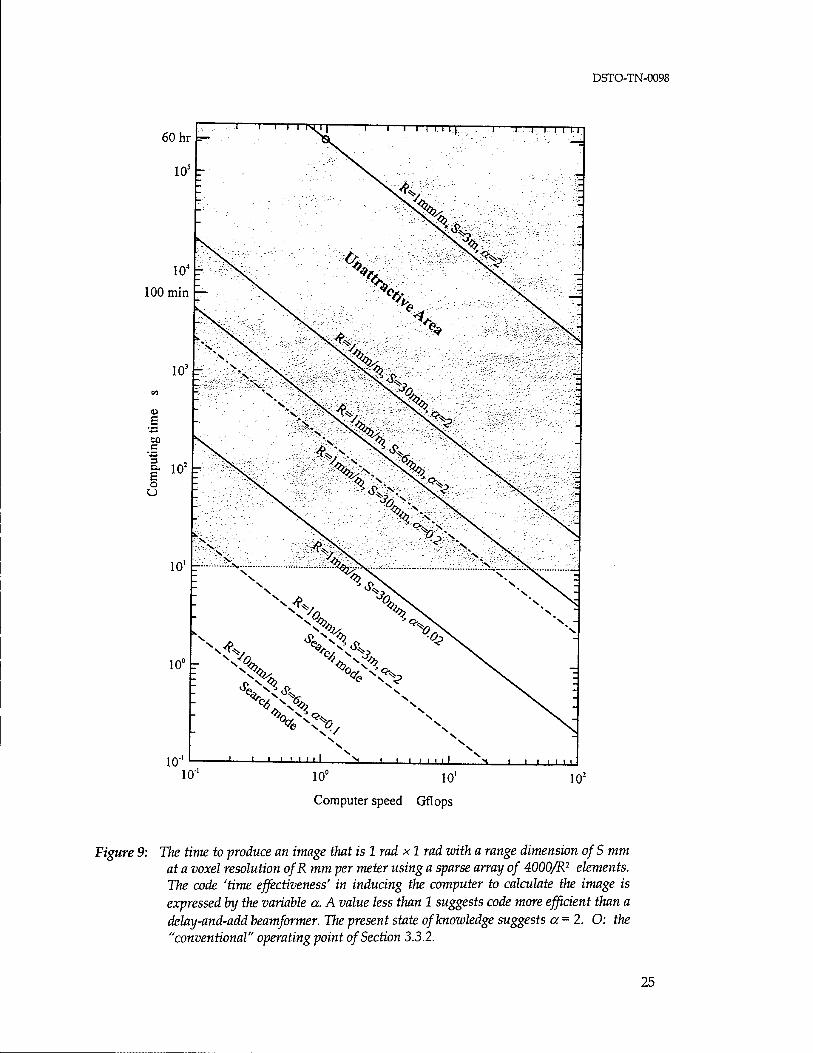
Figure 9: The time to produce an image that is Irad xl rad with a range dimension ofS mm at a voxel resolution ofR mm per meter using a sparse array of 4000/R2 elements. The code 'time effectiveness' in inducing the computer to calculate the image is expressed by the variable a. A value less than 1 suggests code more efficient than a delay-and-add beamformer. The present state of knowledge suggests a = 2. O: the "conventional" operating point of Section 3.3.2.

25

DSTO-TN-0098

today's programmer, while software innovation could produce a large decrease in a.2

The third, or reduced goal, approach, in which one considers only a slice of the volume that one ideally wishes to image, is expressed by the slice thickness S.

The expression used to produce the curves in Figure 9 is 36aS /10N

'""FT' ( > where * is the computation time in seconds, S is the slice thickness in mm, R is the resolution in mm/m and v is the computer speed in Gflops. Here we have imposed a range resolution of R mm. (The coefficient, 36, can be obtained by requiring agreement with Eqn 10 under the conditions S = 4, a = 2. If it is desired to include the time for a sequence of lower-resolution images, according to the left-hand side of Eqn 11, the number 36 should be replaced by 37.2.) It is assumed that lowered resolution is handled by the method of Section 7.5. Thus the resolution R determines the size of the subarray used; and all elements in that subarray are used. Any high-resolution image (R = 1 mm) is therefore a high-quality image (Section 7.4.3). One should note that the lower resolution images use fewer elements in the sparse array and therefore have a worse signal to sidelobe noise ratio. The question of what is an acceptable signal to noise ratio is not addressed in this report. Likewise we have not considered the possibility of varying the number of elements per unit area, which would affect the signal to noise ratio. t

In Figure 9, the area below 1 second is considered suitable for a 'search mode in which a coarse resolution image (say R = 10 mm) is produced frequently (say t = 0.2 s) to guide the ROV and to choose the region in which to position the slice. Possibly the search mode should look at a region of thickness 4 m (range 1-5 m) in order to assist localisation of the target. It can be seen that the search mode could be achieved easily if an algorithm improvement factor of 10 or 20 was achieved, as assumed in the lowest

curve. The area above 10 seconds is shown stippled because in this region it takes an

undesirably long time to produce a high resolution image. The high resolution image is more difficult to achieve than the search mode image, even given the fact that a longer computation time is acceptable. A 10-fold improvement in a (yielding a = 0.2), coupled with a 10-fold increase of computing power over that readily available would, with a slice 30 mm thick, produce a viable solution. This is shown as the dash-dot line in Figure 9.

Figure 9 is provided to allow readers to search for their own compromise.

2 It is recognised that many machines do not neatly fit the separation proposed here between v and a .

For a given coded solution to the beamforming problem on a given machine, the quantity v/a in

Equation (12) is determined, and is the equivalent number of operations of the brute-force method performed per nanosecond. In particular, the separation into v and « may become arbitrary when the machine has fast-access registers distinct from RAM. In the spirit of the discussion, it would then be reasonable to assign the value of v based on operations internal to the system of registers; the value of a

then follows from the known ratio V/ a .

26

DSTO-TN-0098

None of the approaches has been developed to the engineering prototype stage and so the probability of success cannot be provided. The aim of this technical note is to provide a scheme for further work.

9. Acknowledgements

The team drawn from the staff of GEC-Marconi Systems and CSIRO Ultrasonics Laboratory, exemplified by Ian G. Jones and David Robinson, contributed greatly to the success of the innovation program to date. John Shaw and Mike Bell contributed some of the ideas in this report. The task manager was Jim Thompson.

10. References

Blair, D.G. (1993). Array Design: Literature Survey for a High-Resolution Imaging Sonar System-Part 1 (MRL Technical Note MRL-TN-658). Melbourne: DSTO Materials Research Laboratory.

Blair, D.G. (1997). Underwater Acoustic Imaging: A Computing Hardware Approach to Rapid Processing (DSTO Technical Note DSTO-TN-0099). Melbourne: Aeronautical and Maritime Research Laboratory.

Blair, D.G., Bedwell, L, Anstee, S.D. and Li, Y. (1994) Use of a Random Array for High- Resolution Underwater Acoustic Imaging. Proceedings of the International Conference on Underwater Acoustics. Darlinghurst, NSW: Australian Acoustic Society.

Fenton, D. (1989). The Australian Fast Delivery Processor for the Synthetic Aperture Radar ofESR-1. Proceedings of the 5th National Space Engineering Symposium, Canberra. Institution of Engineers Australia.

Guan, L. and Perry, S.W. (1996). Develop 3D Acoustic Imaging Technology: Extracting Objects from Underwater Acoustic Images. Sydney: University of Sydney, Dept. of Elec. Eng.

Jones, I.S.F. (1994). High Resolution Underwater Imaging. Proceedings of the Inter- national Conference on Underwater Acoustics. Darlinghurst, NSW: Australian Acoustic Society.

Jones, I.S.F. (1996). Underwater Acoustic Imaging Innovation Program (DSTO Technical Note DSTO-TN-0065). Melbourne: Aeronautical and Maritime Research Laboratory.

Thuraisingham, R.A. (1994a). Models to Estimate High Frequency Acoustic Scattering Due to Thermal Fine- and Micro-structure of the Ocean (DSTO Research Report DSTO-RR- 0001). Melbourne: Aeronautical and Maritime Research Laboratory.

27

DSTO-TN-0098

Thuraisingham, R.A. (1994b). Theoretical Estimates of High Frequency Acoustic Attenuation and Backscattering from Suspended Sand Particles in tlte Ocean and in an Estuary (DSTO Technical Report DSTO-TR-0078). Melbourne: Aeronautical and Maritime Research Laboratory.

Ziomek, L.J. (1985). Underwater Acoustics: A Linear Systems Theory Approach. New York: Academic Press.

28

DISTRIBUTION LIST

Underwater Acoustic Imaging: Rapid Signal Processing David G. Blair and Ian S. F. Jones

AUSTRALIA

DEFENCE ORGANISATION

Task Sponsor DGFD(Sea)

S&T Program Chief Defence Scientist | FAS Science Policy f shared copy AS Science Corporate Management >

Director General Science Policy Development Counsellor Defence Science, London (Doc Data Sheet) Counsellor Defence Science, Washington (Doc Data Sheet) Scientific Adviser to MRDC Thailand (Doc Data Sheet) Director General Scientific Advisers and Trials/Scientific Adviser Policy and Command (shared copy) Navy Scientific Adviser (3 copies) Scientific Adviser - Army (Doc Data Sheet

and distribution list only) Air Force Scientific Adviser Director Trials

Alan Burgess, ESRL Salisbury Garry Newsam, WASD Salisbury

Aeronautical and Maritime Research Laboratory Director

Chief of Maritime Operations Division Dr A Theobald (Research Leader), MOD Sydney Dr B Ferguson, MOD Sydney Dr D Wyllie (Task Manager), MOD Sydney Mr JL Thompson, 52 Stokes Ave, Asquith, NSW 2077 Stuart Anstee, MOD Sydney Ranjit Thuraisingham, MOD Sydney John Shaw, MOD Sydney Mike Bell, MOD Sydney Doug Cato, MOD Sydney John Riley, MOD Salisbury David Leibing, MOD Salisbury Ross Barrett, MOD Salisbury Warren Marwood, MOD Salisbury

Dr I.S.F. Jones, C/- Ocean Technology Group, J05, University of Sydney, NSW 2006 15 copies Dr D.G. Blair, MOD Sydney 25 copies

DSTO Library Library Fishermens Bend Library Maribyrnong Library Salisbury (2 copies) Australian Archives Library, MOD, Pyrmont (2 copies) Library, MOD, HMAS Stirling

Capability Development Division Director General Maritime Development Director General Land Development (Doc Data Sheet only) Director General C3I Development (Doc Data Sheet only)

Navy SO (Science), Director of Naval Warfare, Maritime Headquarters Annex,

Garden Island, NSW 2000 (Doc Data Sheet and distribution list only) Mine Warfare Systems Centre, PD MHI, PD MHC, PD

Army ABCA Office, G-l-34, Russell Offices, Canberra (4 copies) SO (Science), DJFHQ(L), MILPO Enoggera, Queensland 4051 (Doc Data Sheet only) NAPOC QWG Engineer NBCD c/- DENGRS-A, HQ Engineer Centre Liverpool

Military Area, NSW 2174 (Doc Data Sheet only)

Intelligence Program DGSTA Defence Intelligence Organisation

Corporate Support Program (libraries} OIC TRS, Defence Regional Library, Canberra Officer in Charge, Document Exchange Centre (DEC), 1 copy DEC also requires: *US Defence Technical Information Center, 2 copies *UK Defence Research Information Centre, 2 copies *Canada Defence Scientific Information Service, 1 copy *NZ Defence Information Centre, 1 copy National Library of Australia, 1 copy

UNIVERSITIES AND COLLEGES

Australian Defence Force Academy Library Head of Aerospace and Mechanical Engineering

Senior Librarian, Hargrave Library, Monash University Librarian Flinders University

OTHER ORGANISATIONS

NASA (Canberra) AGPS Mr Francois Duthoit, Head of Engineering, Thomson Marconi Sonar, 274

Victoria Rd, Rydalmere, NSW 2116 (4 copies) Dr Graham Mountford, Project Manager AMI, Thomson Marconi Sonar, 274 Victoria Rd, Rydalmere, NSW 2116 (10 copies) Dr Donald Mclean, CSIRO Division of Telecommunications and Industrial Physics, Bradfield Rd, West Lindfield, NSW 2070 (3 copies) Dr Ling Guan, Dept. of Electrical Engineering, University of Sydney, NSW 2006 Dr David Robinson, 383 Burraneer Rd, Coomba Park, NSW 2428 Dr Andrew Madry, Radiology, Westmead Hospital, Westmead, NSW 2145 Mr Alex Au, Ocean Technology Group, J05, University of Sydney, NSW 2006

OUTSIDE AUSTRALIA

ABSTRACTING AND INFORMATION ORGANISATIONS INSPEC: Acquisitions Section Institution of Electrical Engineers Library, Chemical Abstracts Reference Service Engineering Societies Library, US Materials Information, Cambridge Scientific Abstracts, US Documents Librarian, The Center for Research Libraries, US

INFORMATION EXCHANGE AGREEMENT PARTNERS Acquisitions Unit, Science Reference and Information Service, UK Library - Exchange Desk, National Institute of Standards and Technology, US

SPARES (5 copies)

Total number of copies: 106

Page classification: UNCLASSIFIED

DEFENCE SCIENCE AND TECHNOLOGY ORGANISATION DOCUMENT CONTROL DATA

2. TITLE

Underwater Acoustic Imaging: Rapid Signal Processing

4. AUTHOR(S)

David G. Blair and Ian S. F. Jones

6a. DSTO NUMBER DSTO-TN-0098

8. FILE NUMBER 510/207/0713

6b. AR NUMBER AR-010-280

9. TASK NUMBER ADS 97/045

1. PRIVACY MARKING/CAVEAT (OF DOCUMENT)

3. SECURITY CLASSIFICATION (FOR UNCLASSIFIED REPORTS THAT ARE LIMITED RELEASE USE (L) NEXT TO DOCUMENT CLASSIFICATION)

Document Title Abstract

U U U

5. CORPORATE AUTHOR

Aeronautical and Maritime Research Laboratory PO Box 4331 Melbourne Vic 3001 Australia

6c. TYPE OF REPORT Technical Note

10. TASK SPONSOR DGMD

13. DOWNGRADING/DELIMITING INSTRUCTIONS

7. DOCUMENT DATE April 1998

11. NO. OF PAGES 28

12. NO. OF REFERENCES 10

14. RELEASE AUTHORITY

Chief, Maritime Operations Division

15. SECONDARY RELEASE STATEMENT OF THIS DOCUMENT

Approved for public release

OVERSEAS ENQUIRIES OUTSIDE STATED LIMITATIONS SHOULD BE REFERRED THROUGH DOCUMENT EXCHANGE CENTRE, DIS NETWORK OFFICE, DEFT OF DEFENCE, CAMPBELL PARK OFFICES, CANBERRA ACT 2600 16. DELIBERATE ANNOUNCEMENT

No Limitations

17. CASUAL ANNOUNCEMENT Yes 18. DEFTEST DESCRIPTORS

Signal processing, Beam forming, Sonar arrays, Real time operations

19. ABSTRACT An innovation program to develop an underwater acoustic imaging system able to resolve objects down to millimetre resolution in turbid waters is under way. The defence need is for the identification of minelike objects. This report reviews options for the signal processing or bearriorming stage of the program. An image consisting of 3xl09 voxels (volume pixels) could be formed by a summation of the voltages from 4000 sensor elements, each taken from the element's voltage stream at the appropriate time. With a suitable allowance (factor of 9) for calculating the time delays, it appears at first sight that 9xl.2xl013 operations would be required. The problem is to calculate a three-dimensional image of adequate quality in the shortest time at the least cost. A hierarchical structure of options is developed in an attempt to capture all possibilities. At the top level, three approaches are identified. First, the use of appropriate hardware, such as computers with parallelism. Second, a reduction in the number of operations (a 'software' solution). And third, the defining of a suitable reduced goal, which appears to come down to the imaging of a subvolume of the original volume that contains the object of interest. Each of these three approaches is divided into suboptions; these are discussed in detail to bring out difficulties and advantages.

Page classification: UNCLASSIFIED

^

DSTO* AUSTRALIA

AERONAUTICAL AND MARITIME RESEARCH LABORATORY GPO BOX 4331 MELBOURNE VICTORIA 3001

AUSTRALIA, TELEPHONE (03) 9626 7000

n

n >

z o

a CO —i O

o o o CO

> TO

I o o 00 o > -o 7V

o o 00