UnderStandingAmericaStudy

WEIGHTING PROCEDURE

9/1/2017

2

Contents Introduction .................................................................................................................................................. 3

1. Sampling .................................................................................................................................................... 3

1.1. Special Purpose Samples .................................................................................................................... 4

2. Weighting .................................................................................................................................................. 5

2.1. Step 1: Base Weights .......................................................................................................................... 5

2.2. Step 2: Post-stratification Weights ..................................................................................................... 6

2.3. Categorization and Imputation of Variables ....................................................................................... 8

2.4. Raking/Trimming Algorithm ............................................................................................................... 9

2.5. Final Post-stratification Weights ....................................................................................................... 11

Default Weights ....................................................................................................................................... 11

Custom Weights ...................................................................................................................................... 12

Weighting Output .................................................................................................................................... 13

3

INTRODUCTION

This document provides details of the weighting procedures and benchmark distributions used to

create final sample weights for data sets collected by the Center for Economic and Social

Research’s Understanding America Study internet panel.1

This version (September 2017) supersedes previous versions published on the UAS website. It

differs from previous ones mainly in providing details of a revised weighting protocol. In this new

procedure, we implement a two-step process where we first compute base weights, which correct

for unequal probabilities of sampling UAS members, and then generate final, post-stratification

weights, which align the sample of each study to the reference population along certain socio-

economic dimensions.

Sample weights provided before September 2017 are based on the previous weighting procedure,

which is described here.

1. SAMPLING

In this section, we provide a summary of UAS’s sampling procedures as background for our

weighting protocol. For a full description of the UAS sampling procedure, click here. For a full

description of the UAS recruitment procedures, please click here. UAS documents and data are

online at uasdata.usc.edu.

The UAS is a nationally representative panel of U.S. households recruited through Address Based

Sampling (ABS). Eligible individuals are all adults in the contacted household aged 18 and older.

Sampling in the UAS is done in batches. The first batch (batch 1) is a simple random sample of

individuals from the ASDE Survey Sampler database. Subsequent recruitment batches (batches 5-

12) are selected based on an algorithm developed by Center for Economic and Social Research

(CESR) researchers called Sequential Importance Sampling (SIS). This is a type of adaptive sampling

1 Mick Couper and Jon Krosnick have provided insightful and valuable comments throughout the development of the UAS weighting procedure.

4

that allows to refresh the panel in such a way that its demographic composition moves closer to

the population composition.

Specifically, before sampling an additional batch, the SIS algorithm computes the unweighted

distributions of specific demographic characteristics (e.g., sex, age, marital status and education)

in the UAS at that point in time. It then assigns to each zip code a non-zero probability of being

drawn, which is an increasing function of the degree of “desirability” of the zip code. The degree

of desirability is a measure of how much, given its population characteristics, a zip code is expected

to move the current distributions of demographics in the UAS towards those of the U.S.

population. For example, if at a particular point in time the UAS panel underrepresents females

with high school degree, zip codes with a relatively high proportion of females with high school

degree receive a higher probability of being sampled.

The SIS is implemented iteratively. That is, after selecting a zip code, the distributions of

demographics in the UAS are updated according to the expected contribution of this zip code

towards the panel’s representativeness, updated measures of desirability are computed and new

sampling probabilities for all other zip codes are defined. Such procedure provides a list of zip

codes to be sampled. For each zip code in this list, 40 addresses are then randomly sampled from

the USPS database. The implementation of the SIS algorithm implies that the marginal probability

of drawing each zip code depends on the composition of the UAS panel at a particular point in

time, but also on the unknown response probabilities of selected households in that zip code.

Hence, the marginal probability of drawing each zip code is not known ex ante and cannot be used

to construct design weights. The weighting procedure described below corrects for the unequal

sampling probabilities generated by the SIS algorithm.

1.1. Special Purpose Samples

The UAS also includes two special purpose samples – a sub-panel of Native Americans and a sub-

panel of Los Angeles County residents – for which different sampling procedures are adopted. The

sample of Native Americans (batches 2 and 3) is recruited through ABS, targeting zip codes with a

higher proportion of Native Americans. In this case, eligible individuals are all Native American

adults in the contacted household, aged 18 and older. Recruitment of the first special purpose

sample of Los Angeles County residents (batch 4) is based on birth records information from the

State of California. Later special purpose samples of Los Angeles County residents (batches 13 and

14 as of August 2017) are again recruited through ABS.

5

In what follows, we indicate with 𝑆𝑐𝑜𝑟𝑒 the nationally representative core sample and with 𝑆𝑠𝑝𝑒𝑐𝑖𝑎𝑙

the special purpose samples.

2. WEIGHTING

In the UAS, sample weights are survey-specific. They are provided with each UAS survey and are

meant to make each survey data set representative of the reference U.S. population with respect

to a pre-defined set of socio-demographic variables. Sample weights are constructed in two steps.

In a first step, a base weight is created to account for unequal probabilities of sampling zip codes

produced by the SIS algorithm and to reflect the probability of a household being sampled,

conditional on its zip code being sampled. In a second step, final post-stratification weights are

generated to correct for differential non-response rates and to bring the final survey sample in

line with the reference population as far as the distribution of key variables of interest is

concerned.

Sample weights are constructed only for the nationally representative core sample.

UAS members belonging to the special purpose samples of Native Americans and Los Angeles

County residents have zero base weight and zero final post-stratification weight.

In what follows, we indicate by 𝑁 = 𝑁𝑐 + 𝑁𝑠𝑝 the total survey sample size, where 𝑁𝑐 is the

number of respondents belonging to the nationally representative core sample, who receive a

non-zero weight, and 𝑁𝑠𝑝 is the number of respondents belonging to the special purpose samples,

who receive a zero weight.

2.1. Step 1: Base Weights

In this first step, a base weight is generated to correct for unequal probabilities of sampling zip

codes produced by the SIS algorithm and to account for the probability of sampling households

conditional on their zip code being sampled.

More precisely, to compute the base weight, the unit of analysis is a zip code. We estimate a logit

model for the probability that a zip code is sampled as a function of its characteristics such as

Census region, urbanicity, population size, as well as sex, race, age, marital status and education

composition. Estimation is carried out on an American Community Survey (ACS) file that contains

6

5-year average characteristics at the zip code level, with urbanicity derived from 2010 Urban Area

to ZIP Code Tabulation Area (ZCTA) Relationship File of the U.S. Census Bureau and merged to

this.2 The outcome of this logit model is an estimate of the marginal probability of a zip code being

sampled, which, because of the implementation of the SIS algorithm, is not known ex ante.

We indicate by 𝑤1𝑏 the inverse of the logit estimated probability of sampling each zip code.

Next, for each sampled zip code, the ratio of the number of households in the zip code to the

number of sampled households within the zip code is computed. This is denoted by 𝑤2𝑏.

For the first recruitment batch (batch 1), which is a simple random sample of addresses from the

U.S. population and does not use the SIS algorithm, we use (without loss of generality) 𝑤1𝑏 =

𝑤2𝑏 = 1 instead. The base weight is a zip code level weight defined as:

𝑏𝑎𝑠𝑒 𝑤𝑒𝑖𝑔ℎ𝑡 = 𝑤1𝑏 × 𝑤2

𝑏 × 𝑎,

where 𝑎 is a correction factor such that the sum of the base weights is equal to the number of all

selected households (if all of them respond). This number is equal to the size of the first

recruitment batch (10,000) and to the number of sampled zip codes times 40 (the number of

sampled households within each drawn zip code) for all subsequent recruitment batches (batches

5-12). Hence, the correction factors takes two values, one for the first recruitment batch and one

of all subsequent recruitment batches referring to the nationally representative core sample.

UAS members belonging to the nationally representative core sample are assigned a base weight,

computed as described above, depending on the zip code where they reside at the time of

recruitment.

UAS members belonging to the special purpose samples of Native Americans and Los Angeles

County residents are assigned a base weight of zero.

2.2. Step 2: Post-stratif ication Weights

The execution of the sampling process for a survey is typically less than perfect. Even if the sample

of panel members invited to take a survey is representative of the population along a series of

2 Strictly speaking, all files from the U.S. Census Bureau use "zip code tabulation area" (zcta), which is based on, but not identical to, USPS's definition of zip codes. We ignore the distinction between the two.

7

dimensions, the sample of actual respondents may exhibit discrepancies because of differences in

response rates across groups and/or other issues related to the fielding time and content of the

survey. A second layer of weighting is therefore needed to align the final survey sample to the

reference population as far as the distribution of key variables is concerned.

In this second step, we perform raking weighting (also known as iterative marginal weighting) and

assign weights to survey respondents belonging to the nationally representative core sample such

that the weighted distributions of specific socio-demographic variables in the survey sample match

their population counterparts (benchmark or target distributions).

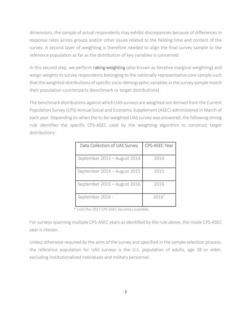
The benchmark distributions against which UAS surveys are weighted are derived from the Current

Population Survey (CPS) Annual Social and Economic Supplement (ASEC) administered in March of

each year. Depending on when the to-be-weighted UAS survey was answered, the following timing

rule identifies the specific CPS-ASEC used by the weighting algorithm to construct target

distributions:

Data Collection of UAS Survey CPS-ASEC Year

September 2013 – August 2014 2014

September 2014 – August 2015 2015

September 2015 – August 2016 2016

September 2016 - 2016*

* Until the 2017 CPS-ASEC becomes available.

For surveys spanning multiple CPS-ASEC years as identified by the rule above, the mode CPS-ASEC

year is chosen.

Unless otherwise required by the aims of the survey and specified in the sample selection process,

the reference population for UAS surveys is the U.S. population of adults, age 18 or older,

excluding institutionalized individuals and military personnel.

8

2.3. Categorization and Imputation of Variables

For post-stratification weighting purposes, we use demographic information taken from the most

recent My Household survey, which is answered by all active UAS members every quarter. With

the exception of age and number of household members, all other socio-demographic variables

in the My Household survey are categorical and some, such as education and income, take values

in a relatively large set. We recode all the variables used in the weighting procedure into new

categorical variables with no more than 5 categories. The aim of limiting the categories is to

prevent these variables from forming strata containing a very small fraction of the sample (less

than 5%), which may cause sample weights to exhibit considerable variability.

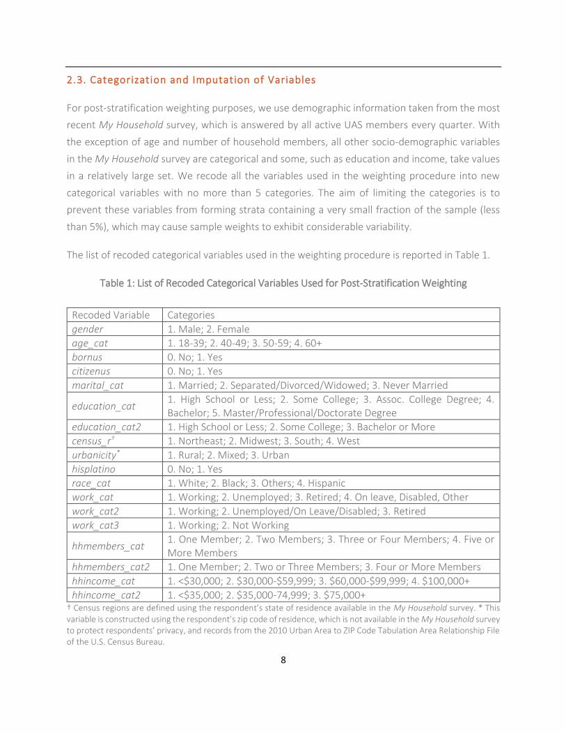
The list of recoded categorical variables used in the weighting procedure is reported in Table 1.

Table 1: List of Recoded Categorical Variables Used for Post-Stratification Weighting

Recoded Variable Categories

gender 1. Male; 2. Female

age_cat 1. 18-39; 2. 40-49; 3. 50-59; 4. 60+

bornus 0. No; 1. Yes

citizenus 0. No; 1. Yes

marital_cat 1. Married; 2. Separated/Divorced/Widowed; 3. Never Married

education_cat 1. High School or Less; 2. Some College; 3. Assoc. College Degree; 4. Bachelor; 5. Master/Professional/Doctorate Degree

education_cat2 1. High School or Less; 2. Some College; 3. Bachelor or More

census_r† 1. Northeast; 2. Midwest; 3. South; 4. West

urbanicity* 1. Rural; 2. Mixed; 3. Urban

hisplatino 0. No; 1. Yes

race_cat 1. White; 2. Black; 3. Others; 4. Hispanic

work_cat 1. Working; 2. Unemployed; 3. Retired; 4. On leave, Disabled, Other

work_cat2 1. Working; 2. Unemployed/On Leave/Disabled; 3. Retired

work_cat3 1. Working; 2. Not Working

hhmembers_cat 1. One Member; 2. Two Members; 3. Three or Four Members; 4. Five or More Members

hhmembers_cat2 1. One Member; 2. Two or Three Members; 3. Four or More Members

hhincome_cat 1. <$30,000; 2. $30,000-$59,999; 3. $60,000-$99,999; 4. $100,000+

hhincome_cat2 1. <$35,000; 2. $35,000-74,999; 3. $75,000+ † Census regions are defined using the respondent’s state of residence available in the My Household survey. * This variable is constructed using the respondent’s zip code of residence, which is not available in the My Household survey to protect respondents’ privacy, and records from the 2010 Urban Area to ZIP Code Tabulation Area Relationship File of the U.S. Census Bureau.

9

Before implementing the post-stratification weighting procedure, we employ the following

imputation scheme to replace missing values of recoded socio-demographic variables.

When actual age is missing, the variable agerange, available in the My Household survey,

is used to impute age_cat. If agerange is also missing, the variable age_cat is replaced with

the gender-specific sample mode, depending on the respondent’s gender.

For binary indicators, such as bornus, citizenus, and hisplatino, missing values are imputed

using a logistic regression.

For ordered categorical variables, such as education_cat, education_cat2,

hhmembers_cat, hhmembers_cat2, hhincome_cat and hhincome_cat2, missing values are

imputed using an ordered logistic regression.

For non-ordered categorical variables, such as marital_cat, race_cat and work_cat,

census_r, missing values are imputed using a multinomial logistic regression.

Imputations are performed sequentially. That is, once age_cat has been imputed (if missing), the

variable with the smallest number of missing values is the first one to be imputed by means of a

regression featuring gender and age_cat as regressors. This newly imputed variable is then added

to the set of regressors to impute the variable with the second smallest number of missing values.

The procedure continues in this fashion until the variable with the most missing values is imputed

using information on all other available socio-demographic variables.

Each weighted UAS survey data set contains a binary variable, imputation_flag, indicating whether

any of the recoded socio-economic variables listed in Table 1 and used within the post-

stratification weighting procedure has been imputed.

2.4. Raking/Trimming Algorithm

We adopt a raking algorithm to generate post-stratification weights. This procedure involves the

comparison of target population relative frequencies and actually achieved sample relative

frequencies on a number of socio-demographic variables independently and sequentially. More

precisely, starting from the base weights as described in section 2.1, at each iteration of the

algorithm weights are proportionally adjusted so that the distance between survey and population

marginal distributions of each selected socio-demographic variable (or raking factor) decreases.

10

The algorithm stops when survey and population distributions are perfectly aligned. A maximum

of 50 iterations is allowed for perfect alignment of survey and population distributions to be

achieved. If the process does not converge within 50 iterations, no sample weights are returned

and attempts using different raking factors are made.

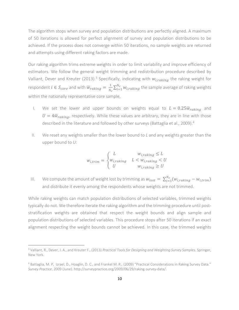
Our raking algorithm trims extreme weights in order to limit variability and improve efficiency of

estimators. We follow the general weight trimming and redistribution procedure described by

Valliant, Dever and Kreuter (2013).3 Specifically, indicating with 𝑤𝑖,𝑟𝑎𝑘𝑖𝑛𝑔 the raking weight for

respondent 𝑖 ∈ 𝑆𝑐𝑜𝑟𝑒 and with �̅�𝑟𝑎𝑘𝑖𝑛𝑔 = 1

𝑁𝑐∑ 𝑤𝑖,𝑟𝑎𝑘𝑖𝑛𝑔

𝑁𝑐𝑖=1 the sample average of raking weights

within the nationally representative core sample,

I. We set the lower and upper bounds on weights equal to 𝐿 = 0.25�̅�𝑟𝑎𝑘𝑖𝑛𝑔 and

𝑈 = 4�̅�𝑟𝑎𝑘𝑖𝑛𝑔, respectively. While these values are arbitrary, they are in line with those

described in the literature and followed by other surveys (Battaglia et al., 2009).4

II. We reset any weights smaller than the lower bound to L and any weights greater than the

upper bound to U:

𝑤𝑖,𝑡𝑟𝑖𝑚 = {

𝐿 𝑤𝑖,𝑟𝑎𝑘𝑖𝑛𝑔 ≤ 𝐿

𝑤𝑖,𝑟𝑎𝑘𝑖𝑛𝑔 𝐿 < 𝑤𝑖,𝑟𝑎𝑘𝑖𝑛𝑔 < 𝑈

𝑈 𝑤𝑖,𝑟𝑎𝑘𝑖𝑛𝑔 ≥ 𝑈

III. We compute the amount of weight lost by trimming as 𝑤𝑙𝑜𝑠𝑡 = ∑ (𝑤𝑖,𝑟𝑎𝑘𝑖𝑛𝑔𝑁𝑐𝑖=1 − 𝑤𝑖,𝑡𝑟𝑖𝑚)

and distribute it evenly among the respondents whose weights are not trimmed.

While raking weights can match population distributions of selected variables, trimmed weights

typically do not. We therefore iterate the raking algorithm and the trimming procedure until post-

stratification weights are obtained that respect the weight bounds and align sample and

population distributions of selected variables. This procedure stops after 50 iterations if an exact

alignment respecting the weight bounds cannot be achieved. In this case, the trimmed weights

3 Valliant, R., Dever, J. A., and Kreuter F., (2013) Practical Tools for Designing and Weighting Survey Samples. Springer, New York.

4 Battaglia, M. P, Izrael, D., Hoaglin, D. C., and Frankel M. R., (2009) “Practical Considerations in Raking Survey Data.” Survey Practice, 2009 (June). http://surveypractice.org/2009/06/29/raking-survey-data/.

11

will ensure the exact match between survey and population relative frequencies, but may take

values outside the interval defined by the pre-specified lower and upper bounds.

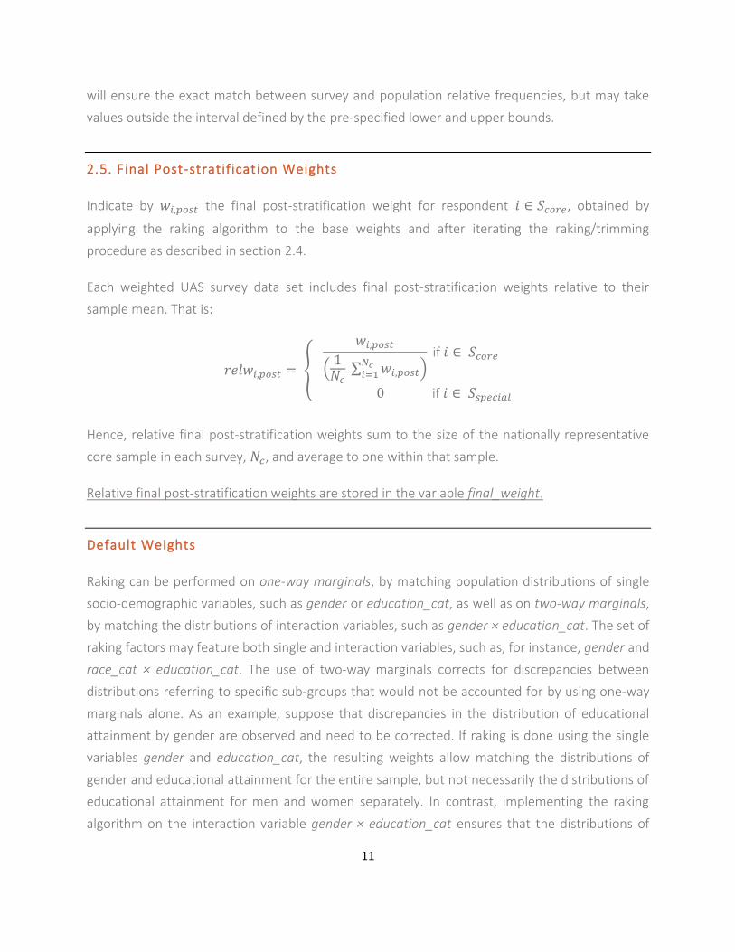
2.5. Final Post-stratification Weights

Indicate by 𝑤𝑖,𝑝𝑜𝑠𝑡 the final post-stratification weight for respondent 𝑖 ∈ 𝑆𝑐𝑜𝑟𝑒, obtained by

applying the raking algorithm to the base weights and after iterating the raking/trimming

procedure as described in section 2.4.

Each weighted UAS survey data set includes final post-stratification weights relative to their

sample mean. That is:

𝑟𝑒𝑙𝑤𝑖,𝑝𝑜𝑠𝑡 = {

𝑤𝑖,𝑝𝑜𝑠𝑡

(1

𝑁𝑐 ∑ 𝑤𝑖,𝑝𝑜𝑠𝑡

𝑁𝑐𝑖=1 )

if 𝑖 ∈ 𝑆𝑐𝑜𝑟𝑒

0 if 𝑖 ∈ 𝑆𝑠𝑝𝑒𝑐𝑖𝑎𝑙

Hence, relative final post-stratification weights sum to the size of the nationally representative

core sample in each survey, 𝑁𝑐, and average to one within that sample.

Relative final post-stratification weights are stored in the variable final_weight.

Default Weights

Raking can be performed on one-way marginals, by matching population distributions of single

socio-demographic variables, such as gender or education_cat, as well as on two-way marginals,

by matching the distributions of interaction variables, such as gender × education_cat. The set of

raking factors may feature both single and interaction variables, such as, for instance, gender and

race_cat × education_cat. The use of two-way marginals corrects for discrepancies between

distributions referring to specific sub-groups that would not be accounted for by using one-way

marginals alone. As an example, suppose that discrepancies in the distribution of educational

attainment by gender are observed and need to be corrected. If raking is done using the single

variables gender and education_cat, the resulting weights allow matching the distributions of

gender and educational attainment for the entire sample, but not necessarily the distributions of

educational attainment for men and women separately. In contrast, implementing the raking

algorithm on the interaction variable gender × education_cat ensures that the distributions of

12

educational attainment for men and women are matched to their population counterparts.

Moreover, since two-way marginals subsume one-way marginals, using the interaction variable

gender × education_cat also guarantees that the distributions of gender and education for the

entire sample are matched to their population counterparts.

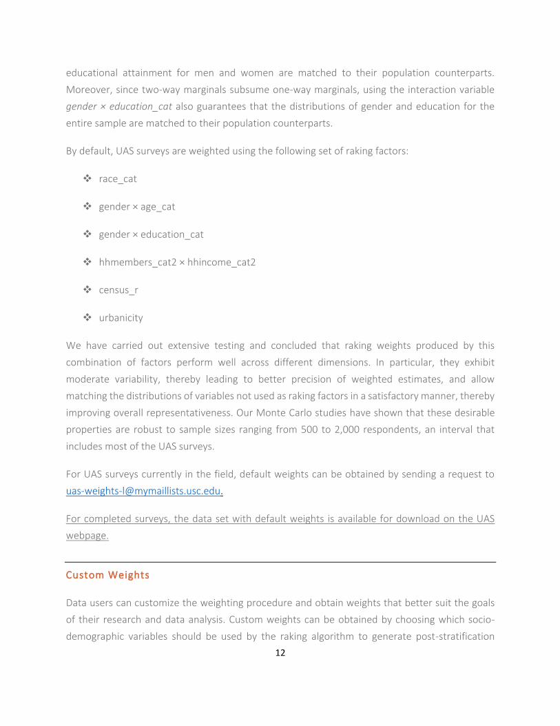
By default, UAS surveys are weighted using the following set of raking factors:

race_cat

gender × age_cat

gender × education_cat

hhmembers_cat2 × hhincome_cat2

census_r

urbanicity

We have carried out extensive testing and concluded that raking weights produced by this

combination of factors perform well across different dimensions. In particular, they exhibit

moderate variability, thereby leading to better precision of weighted estimates, and allow

matching the distributions of variables not used as raking factors in a satisfactory manner, thereby

improving overall representativeness. Our Monte Carlo studies have shown that these desirable

properties are robust to sample sizes ranging from 500 to 2,000 respondents, an interval that

includes most of the UAS surveys.

For UAS surveys currently in the field, default weights can be obtained by sending a request to

uas-weights-l@mymaillists.usc.edu.

For completed surveys, the data set with default weights is available for download on the UAS

webpage.

Custom Weights

Data users can customize the weighting procedure and obtain weights that better suit the goals

of their research and data analysis. Custom weights can be obtained by choosing which socio-

demographic variables should be used by the raking algorithm to generate post-stratification

13

weights. Custom weights requests should be sent to uas-weights-l@mymaillists.usc.edu, alongside

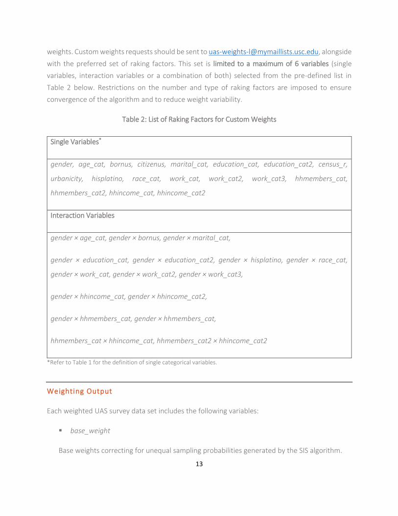
with the preferred set of raking factors. This set is limited to a maximum of 6 variables (single

variables, interaction variables or a combination of both) selected from the pre-defined list in

Table 2 below. Restrictions on the number and type of raking factors are imposed to ensure

convergence of the algorithm and to reduce weight variability.

Table 2: List of Raking Factors for Custom Weights

Single Variables*

gender, age_cat, bornus, citizenus, marital_cat, education_cat, education_cat2, census_r,

urbanicity, hisplatino, race_cat, work_cat, work_cat2, work_cat3, hhmembers_cat,

hhmembers_cat2, hhincome_cat, hhincome_cat2

Interaction Variables

gender × age_cat, gender × bornus, gender × marital_cat,

gender × education_cat, gender × education_cat2, gender × hisplatino, gender × race_cat,

gender × work_cat, gender × work_cat2, gender × work_cat3,

gender × hhincome_cat, gender × hhincome_cat2,

gender × hhmembers_cat, gender × hhmembers_cat,

hhmembers_cat × hhincome_cat, hhmembers_cat2 × hhincome_cat2

*Refer to Table 1 for the definition of single categorical variables.

Weighting Output

Each weighted UAS survey data set includes the following variables:

base_weight

Base weights correcting for unequal sampling probabilities generated by the SIS algorithm.

14

imputation_flag

A binary variable indicating whether any of the variables used within the post-stratification

weighting procedure has been imputed.

final_weight

Relative final post-stratification weights ensuring representativeness of the survey sample with

respect to key pre-selected demographic variables. They are non-zero for respondents

belonging to the nationally representative core sample and zero for respondents belonging to

special purpose samples.