Understanding User Economic Behavior in the City UsingLarge-scale Geotagged and Crowdsourced Data

Yingjie ZhangHeinz College

Carnegie Mellon UniversityPittsburgh, PA 15213, USA

yingjie@cmu.edu

Beibei LiHeinz College

Carnegie Mellon UniversityPittsburgh, PA 15213, USA

beibeili@andrew.cmu.edu

Jason HongSchool of Computer ScienceCarnegie Mellon UniversityPittsburgh, PA 15213, USAjasonh@cs.cmu.edu

ABSTRACTThe pervasiveness of mobile technologies today have facili-tated the creation of massive crowdsourced and geotaggeddata from individual users in real time and at different loca-tions in the city. Such ubiquitous user-generated data allowus to infer various patterns of human behavior, which helpus understand the interactions between humans and cities.In this study, we focus on understanding users economic be-havior in the city by examining the economic value fromcrowdsourced and geotaggged data. Specifically, we extractmultiple traffic and human mobility features from publiclyavailable data sources using NLP and geo-mapping tech-niques, and examine the effects of both static and dynamicfeatures on economic outcome of local businesses. Our studyis instantiated on a unique dataset of restaurant bookingsfrom OpenTable for 3,187 restaurants in New York City fromNovember 2013 to March 2014. Our results suggest thatfoot traffic can increase local popularity and business per-formance, while mobility and traffic from automobiles mayhurt local businesses, especially the well-established chain-s and high-end restaurants. We also find that on averageone more street closure nearby leads to a 4.7% decrease inthe probability of a restaurant being fully booked during thedinner peak. Our study demonstrates the potential of howto best make use of the large volumes and diverse sources ofcrowdsourced and geotagged user-generated data to creatematrices to predict local economic demand in a manner thatis fast, cheap, accurate, and meaningful.

KeywordsGeotagged Social Media, Crowdsourced User Behavior, E-conometrics, Location-Based Service, Economic Analysis,City Demand, Mobility Analytics, NLP

1. INTRODUCTIONRapid urbanization is imposing various urban challenges,

especially increased demand on the city infrastructures andon the quality of services. These challenges call for a specificfocus on urban systems and their interaction with humans

Copyright is held by the International World Wide Web Conference Com-mittee (IW3C2). IW3C2 reserves the right to provide a hyperlink to theauthor’s site if the Material is used in electronic media.WWW 2016, April 11–15, 2016, Montréal, Québec, Canada.ACM 978-1-4503-4143-1/16/04.http://dx.doi.org/10.1145/2872427.2883066.

and businesses. In particular, properties of a city, such astransportation, street facilities, and neighborhood walkabil-ity, and their impacts on human behavior are at the core ofsustainability and local economy. For example, when ma-jor streets in Boston were locked down during the MarathonBombing in April 2013, the estimated costs to local business-es ranged from $250 to $333 million a day [3]. A decrease infoot traffic can have significantly negative impact on storesales. These kinds of economic losses can lead to a negativeeffect on the local economy and can impose a long-term ef-fect on the future sustainability of the urban neighborhoodand quality of life. Therefore, understanding the patternsof human behavior in the city, especially how humans re-spond to city infrastructures and services from an economicperspective is critical in helping policy makers proactivelyimprove city planning for better social welfare.

One major challenge here is in quantifying and measuringthe quality of city infrastructures and services, as it includesmany factors, such as user walkability, street connectivity,traffic conditions, and other urban amenities. These multi-dimensional characteristics make it difficult to quantify andmeasure the service quality in an urban system. Further-more, it reflects a combination of not only the static spatialand social elements in an urban environment, but also thedynamic characteristics of an urban system. This dynamicnature makes it highly unpredictable with regard to its e-conomic impact on human behaviors. In this research, weextract this information by applying NLP and geo-mappingtechniques on large-scale data from Twitter and Foursquare.Using geotagged user-generated data created via mobile andlocation-based services and crowdsourcing channels, we areable to extract the fine-grained information on various real-time traffic conditions, street events and human movementsthat would otherwise be impossible to measure.

Another major challenge in this research lies in measuringthe economic impacts of city infrastructures and serviceson human behavior. Little work has been done to examinefrom a social and economic perspective of such data to inferrelationship between humans and cities. This is the mainfocus of our paper. In particular, using methods devisedfrom economics, we focus on understanding the economicbehavior of users in the city by examining the economic valuefrom such large-scale and fine-grained information extractedfrom geotagged and crowdsourced channels.

Combining spatial, traffic and human mobility analyticswith economic analyses, our research goals are two-fold:

205

• Extract spatial and socioeconomic features of citiesfrom geotagged and crowdsourced data at large scale;

• Apply econometric models to quantify the causal ef-fects of different features on the economic outcome ofhuman behavior towards local businesses.

We instantiate our study in the context of local restaurants’booking performance by using a unique dataset of restau-rant reservations from OpenTable, a major U.S. restaurantbooking website. The dataset contains complete informationfrom November 2013 to March 2014 for 3,187 restaurants inNew York City. In addition, we use information on neigh-borhood from four main sources across various social medi-a channels and location-based services: (i) social and geo-graphical information about local neighborhoods; (ii) streetevents and construction information collected from NYC’sonline map portal; (iii) human mobility information from ap-proximately 380,000 Foursquare user mobile check-ins; and(iv) traffic-related information extracted from 18,900 indi-vidual geotagged tweets from Twitter.

Our final results show that features extracted from thedigitized and crowdsourced user behavior are informative ininferring local demand. The results show a significant pos-itive impact of human foot traffic on local businesses, andsignificant negative effects due to traffic. Specifically, a 10%increase in the density of human foot traffic increases theprobability of a restaurant being fully booked during dinnerpeak hour by 4%, whereas a 10% increase in real-time trans-portation traffic density can decrease this probability by 5%.We also find that, on average, one more street event or con-struction project nearby can decrease the probability of arestaurant being fully booked during the peak dinner hourby 4.7%. Our econometric methods alleviate the potentialconcerns of endogeneity from different factors in an urbansystem and support our findings from a causal perspective.

Our key contributions can be summarized as follows. (i)We propose a fast and effective way to leverage large-scaledata from geotagged and crowdsourced social media to learnuser economic behavior and local demand in the city. (ii) Tothe best of our knowledge, ours is the first study to quantifythe economic impact of not only static features but also dy-namic features of users’ digitized and crowdsourced behavioron local businesses. Our findings can help local businesses tounderstand the social and economic development of differenturban areas, and to improve marketing strategies by lever-aging large-scale spatial, traffic and human mobility analyticfrom social media. Our results can also help facilitate bet-ter policy decision-making about proactive city planning andimprove the sustainability of urban neighborhoods. Finally,our work also offers an opportunity for incorporating an e-conomic lens into location-based services and geo-mappingservices, which could help improve our understanding of lo-cal areas, as well as local search and local advertising.

2. RELATED WORKWe initiate our research focus on two questions: (i) How

can we efficiently extract features that would potentially af-fect local demand from various available resources, includingsocial media channels and official sources? (ii) How can weuse these characteristics to evaluate the value of informationfrom an economic perspective? To examine these questions,our paper draws from multiple streams of work.

Geotagged and Crowdsourced Data Analysis. With the grow-ing volume of geographic datasets, more and more stud-ies are attracted by the location-based services [16]. Pre-vious studies used various methods to explore this emerg-ing phenomenon from different perspectives, including us-age patterns of location-sharing applications [5]; relation-ship between people [8]; and detection of real-time events[19]. These studies put various methods forward to evaluatethe human mobility patterns. But most of those studies areexploratory analyses, answering what happen and how usersbehave in the real world. They didn’t link their study to theeconomic values while such further-step analysis can benefitthe economic development, or even the entire society.

Economic Values of Users’ Behavior. Understanding the e-conomic and social values is the main focus of researchersin marketing or economic related fields [7]. Due to the lackof data, they limit their studies in the online world. Howev-er, the microeconomics, especially the performance of smallbusinesses, are largely affected by various location-specificfactors. Merely relying on online sources is hard to gaina holistic picture to understand the business mechanism atmicro level. Here, we utilize geotagged and crowdsourceddata to study their economic values for small businesses.

Economics of Location and Urban System. In addition, ourstudy is also closely related to the economics of location andurban system. This stream of research can be traced backto the 1970s [15]. Different studies used various indicatorsto detect the market price [2], best location [10], etc. How-ever, the indicators they used to evaluate the economic val-ues were based on historical records or census data, suchas demographics, crime rates, and climate records. One ofthe disadvantages is that such indicators cannot preciselycapture the real-time performance of an urban system andits impacts. This can potentially present more implicationsfor understanding the relationship between an urban systemand the local economy. More recently, studies from informa-tion systems and urban economics looked at the interactionsbetween new technology and local market [11].

3. DATAOur dataset consists of observations of 3,187 Manhattan

(NYC) restaurants from November 29, 2013 to March 6,2014. The data were collected from multiple sources.

3.1 Data Source Description

3.1.1 Restaurant Reservation DataWe have approximately three months of restaurant reser-

vation data from OpenTable from November 29, 2013 toMarch 6, 2014. This website offers an online network systemto connect reservations between restaurants and consumers.Specifically, the website lists real-time reservation availabil-ity information, given different requested time slots. Ourdataset contains information about reservation availabilityfor a party of two for six different time slots: 6pm, 6:30p-m, 7pm, 7:30pm, 8pm and 8:30pm (peak dining hours). Intotal, we have 312,326 data points.

3.1.2 Geotagged and Crowdsourced DataThe local demand is largely affected by the social and

economic factors in their neighborhoods. To extract thosefactors, we collected crowdsourced and geotagged data basedon three publicly available sources:

206

a)NYC street closure data. We collected street closure da-

ta from the official map portal (gis.nyc.gov/streetclosure/).Every day, it publishes information about street closurescaused by street or intersection construction projects or spe-cial events in Manhattan. After removing duplicate projects,we obtained a total of 3,700 construction projects. Most ofthe projects, which were captured at a granular level, coveronly one to two blocks. This information allowed us to pindown the effects of street closures on nearby restaurants.

b)Foursquare check-ins data. We crawled Foursquare mo-bile check-ins publicly visible on Twitter. Previous researchhas shown the potential of approximating user footprintswith mobile check-ins [16]. We have approximately 380,000mobile user check-ins generated within a 30 miles radiusfrom the center of Manhattan. We used geo-coding toolsto extract the geographical location (i.e., latitude and lon-gitude information) of the check-ins.

c)Traffic-related tweets data. We extracted tweets relat-ed to traffic from Twitter using NLP and geo-coding tech-niques. We conducted this step using two approaches. First,we considered the entire Twitter dataset over the three-month period and extracted traffic-related keywords. Inaddition, we identified and extracted information from in-fluential users on Twitter who tweeted primarily about traf-fic. Specifically, we used all the tweets post by “511 NYCArea (@511NYC)”, whose information is provided by theNew York State Department of Transportation. The tweetsinclude different types of real-time traffic conditions, suchas accidents, heavy traffic, special events, bus delays, etc.We extracted 18,000 traffic tweets that cover our data pe-riod (i.e., 100 days). Again, we were able to extract thegeo-coordinates associated with all these tweets to infer theexact location of each traffic incident.

To link all of the above datasets, we geotagged all datausing Google Map API. Because neither OpenTable datanor street closure data contain geographical coordinates, wefirst translated street addresses into geo-coordinates. Then,we computed the direct distance between each of the pairs:restaurant and restaurant, restaurant and street closure,restaurant and check-ins, and restaurant and traffic tweet-s. Here we consider neighborhood as a 0.5-mile-radius area,which we assume is a walkable distance [4].

Restaurant Characteristics Data. Previous studies show thatonline word-of-mouth does affect restaurants sales becauerestaurants’ quality and popularity can be inferred fromsuch crowdsourced information [18]. Besides, restaurants’inherent characteristics also affect customers’ choices andthe restaurants’ profits. To capture those factors, we ob-tained the restaurants’ characteristics from both OpenTableand Yelp. From OpenTable, we have detailed informationon price level (ranging from 1 to 5), number of reviews, starrating (ranging from 1 to 5) and cuisine type. We also col-lected information about whether the restaurants offer pro-motion points for consumers to redeem OpenTable DiningCheque. To obtain more complete promotion informationfor each restaurant, we crawled restaurants’ promotion datafrom Yelp and matched the Yelp and OpenTable restaurantsbased on their names, street addresses, and geo-tags.

3.1.3 Local Census and Weather DataTo better examine the socio-demographics of neighbor-

hoods and control other possible factors, we collected localpopulation information at zipcode level from the US Census

website (factfinder2.census.gov/), and recorded the av-erage temperature and daily precipitation during the sametime period from Weatherbase (www.weatherbase.com/).

3.2 Feature ExtractionWe created five different sets of features to measure the

characteristics of each restaurant, including four location-related categories and one restaurant-quality-related feature.

3.2.1 Static Spatial FeaturesThis set of features models a restaurant’s static spatial

characteristics (STATIC SPA). Similar to [14], we evaluateit as a vector with four values: location density, popula-tion density, heterogeneity and competitiveness. Formally,a restaurant i has its static spatial features:

STATIC SPAi ={

LOC DENSITYi,HETEROGENEITYi,POP DENSITYi,COMPETITIVENESSi

}. (1)

Density For each restaurant i, we measure its popularityusing the number of nearby restaurants (LOC DENSITYi)and population size (POP DENSITYi). Formally, with thenearby restaurant j ∈ d(i, l) (a disk of radius l aroundrestaurant i), the location density is defined as :

LOC DENSITYi = |j|j ∈ d(i, l)|. (2)

Heterogeneity: Similar to the ideas in [14] we use the entropymeasurement to assess the level of spatial heterogeneity ofan area. Entropy is defined as the expected amount of theinformation from certain events. We apply it into the fre-quency of restaurant types in the area. For example, anarea with only Chinese restaurants has low heterogeneity,whereas a neighborhood with all kinds of Asian restaurantsenjoys a higher heterogeneity. Each restaurant i has its owncuisine type χi. We denote Nχ(i, l) as the number of nearbyrestaurants with cuisine type χ in disk d(i, l), and χ ∈ Γ,where Γ is a set of all cuisine types. We denote N(i, l) asthe total number of restaurants in this area. Formally,

HETEROGENEITYi = −∑χ∈Γ

Nχ(i, l)

N(i, l)× Nχ(i, l)

N(i, l). (3)

The negative sign indicates that a higher level of diversityin terms of cuisine types has a higher heterogeneity value.

Competitiveness: Given the restaurant i with given cui-sine type χi, we measure the proportion of nearby restau-rants of the same cuisine type χi with the total number ofrestaurants within this area. Intuitively, an area with on-ly Chinese restaurants would have a relatively high level ofcompetitiveness because all the restaurants sell similar prod-ucts. The restaurant in the most competitive area has thevalue closest to 1 (which indicates that all the restaurantsin that area offer the same cuisine style).

COMPETITIVENESSi =Nχi(i, l)

N(i, l). (4)

3.2.2 Human Mobility FeaturesAs is well known, walkability is an import concept in

the design of a community [9]. Walking is the most com-mon leisure-time physical activity in the US and has beenfound to have various economic benefits, including urbanneighborhood accessibility, increased efficiency of land useand improved urban livability [17]. In this study, we useFoursquare check-in data to measure this human mobili-ty feature (NEIGH WALK) by tracking both spatial and

207

Table 1: Definition and Statistics Summary of Variables

Variable Definition Mean Std.Err Min MaxPr(FULL) Probability of being full 0.2 0.39 0 1LOC DENSITY Number of restaurants 38.86 2.38 0 620POP DENSITY Population size 22,697.27 1.29 144 110,194COMPETITIVENESS Proportion of same-type restaurants 0.091 0.12 0 0.67HETEROGENEITY Entropy of restaurant types 2.03 1.11 0 3.17MOB DENSITY Total number of mobile check-ins 21.12 3.31 0 1,465SOC STABILITY Consecutive check-ins in the same area 15.8 2.55 0 772IN MOBILITY Incoming flows of mobile check-ins 19.69 2.6 0 608TRA EFF Number of traffic-related tweets 1.67 1.55 0 78ACCIDENT Number of accident-related tweets 0.1 0.38 0 5DISABLED Number of disabled-vehicles-related tweets 0.1 0.38 0 5DELAYS Number of bus-delays-related tweets 0.14 0.48 0 8HEAVYTRAFFIC Number of heavy-traffic-related tweets 0.04 0.26 0 4WEATHER Number of weather-related tweets 0.04 0.32 0 9EVENTS Number of events-related tweets 0.09 0.55 0 9STREET CLO Whether the area has street closures 0.088 0.28 0 1PRICE Price dollar level (OpenTable) 2.53 0.62 2 4RATING Numerical star rating (OpenTable) 4.02 0.39 1 5NUMOFREVIEW Total number of reviews (OpenTable) 40.45 1.24 0 1,451DEALS Whether restaurant has deals on Yelp 0.01 0.11 0 1PROMOTION Whether restaurant in promotion list (OpenTable) 0.15 0.36 0 1GOOGLE TREND Google search volume of each query 4,428.47 37,854.12 0 1,830,000TEMPERATURE Whether temperature is above zero degree. 0.84 0.37 0 1PRECIPITATION Whether precipitation is above zero. 0.58 0.49 0 1HOLIDAY Whether in the holiday season 0.17 0.38 0 1

Number of Observations: 312,326 Time Periods: 11/29/2013-3/8/2014

Data source: New York City, with 0.5-mile-range neighborhoods. Variables are computed at daily level.

temporal characteristics of users’ check-ins. Here, we use(p, t) ∈ C to denote a check-in recorded in place p andat time t, where C is the set of the Foursquare check-insdataset. Specifically, we measure the mobility density, so-cial stability and incoming mobility of the area. This fea-ture vector is based on the data that are collected withina certain period (i.e., one day). Mathematically, we definethat restaurant i’s human mobility features as follows:

NEIGH WALKi ={

MOB DENSITYi,SOC STABILITYi,IN MOBILITYi

}. (5)

Mobile Density: To assess the general popularity of an area,we measure the total number of check-ins collected amongthe neighborhood of restaurant i, within time period T .

MOB DENSITYi = |(p, t)|p ∈ d(i, l), t ∈ T |. (6)

Social Stability: The popularity of an area can be reflect-ed in two ways: whether it can maintain current consumersfor a long period of time and whether it can attract con-sumers from its neighborhoods. Social stability measuresthe first scenario, while incoming mobility evaluates the sec-ond. We use consumers’ consecutive check-in behaviors toassess the stability of current consumers staying in the sameplace. Here, we define Cu ⊂ C as the check-ins subsets ofuser u ∈ U , where U represents the set of all users in ourdata. Formally, by denoting a tuple (pm, tm, pn, tn), and twoconsecutive check-ins (pm, tm), (pn, tn), we have:

SOC STABLITYi =∑u∈U

|{

(pm,tm,pn,tn)∈Cu|pm,pn∈d(i,l),tm,tn inT

} ∣∣∣ (7)

Incoming Mobility: One way to show the popularity of aneighborhood is that it attracts people from other neigh-borhoods can be attracted for shopping and visiting. Thus,not only the ability to maintain consumers, but also the at-traction of potential consumers from other areas, can reflectthe popularity of an area. To capture this factor, we useconsecutive check-in transitions to measure this flow:

IN MOBILITYi =∑u∈U

|{

(pm,tm,pn,tn)∈Cu|pm 6∈d(i,l),pn∈d(i,l),tm,tn∈T

} ∣∣∣ (8)

3.2.3 Dynamic Traffic Efficiency FeaturesTraffic efficiency features (denoted as TRA EFF) measure

the dynamic neighborhood accessibility. Every day, thereare various emergencies leading to the (partial) closure ofcertain streets, such as traffic accidents, traffic jams, busdelays, etc. Such street closure lowers the accessibility of theneighborhood. In our model, we use user-generated contentfrom Twitter to extract the dynamic traffic conditions.

3.2.4 Street Closure (Event, Construction) FeaturesIn addition to traffic emergencies as described above, some

street closures are longer-term, such as road constructionor special city events. We use a street closure feature (de-noted as STREET CLO) to measure the average level ofstreet accessibility within a given neighborhood by captur-ing whether there are any locked-down streets in this neigh-borhood. This dummy variable indicates whether there areevents or street construction projects within a given restau-rant’s neighborhood. Furthermore, rather than using a sim-ple binary variable, we count the exact number of closedstreets and the time length of these closures.

208

3.2.5 Restaurant-Specific FeaturesIn addition to the above factors, restaurant-level hetero-

geneity has non-ignorable effects on the business perfor-mance. In order to control for such effects and to deter-mine a causal effect of urban neighborhood accessibility, webuild a restaurant-specific feature vector (REST SPE) withthree commonly-used elements. We use price level (dividedinto five degrees), star rating level and number of reviews toassess the restaurant’s popularity and quality. Specifically,restaurant i’s restaurant-specific features are denoted:

REST SPEi = {PRICEi,RATINGi,NUMOFREVIEWi}. (9)

Price level: PRICEi denotes the level of the average priceof the restaurant. Based on the data we obtained fromOpenTable, we divide price into five levels, with a higherlevel indicating a higher average price.

Rating: RATINGi represents the quality of the restaurantfrom Opentable. In our dataset, we collected the star levelof each restaurant, as labeled by thousands of consumers.

Comment reviews: NUMOFREVIEWi is the aggregatednumber of reviews about restaurant i on the Opentable web-site, which, to some extent, indicates its popularity.

For a better understanding of variables in our setting, wepresent the definitions and statistics summary of all vari-ables (including the above feature variables, as well as out-come variables and controls in the following model section)in Table 1 and display the statistics summary of the impor-tant continuous variables in Figure 1.

4. ECONOMETRIC MODELINGEconometrics is a well-established statistics technique to

test hypotheses and to predict future changes using econom-ic model. In this paper, our econometric model aims toquantify the causal effects of different features on the eco-nomic outcome of human behavior towards local businesses.

4.1 Panel Data AnalysisBased on our time-series dataset, we use a fixed-effect pan-

el model to estimate the impact of different factors in anurban neighborhood on the restaurant bookings. Our mainmodel can be formalized in the following equation:

Pr(FULL)it = αi + STATIC SPAi · Tt · δ1 + HUMAN MOBit · δ2+ TRA EFFit · δ3 + STREET CLOit · δ4 + REST SPEit · δ5+ Controlsit · φ+ Tt + εit,

(10)

where Pr(FULL)it is the probability that a restaurant i isfull (i.e., no available reservation slots) at day t. The de-pendent variable captures the restaurant’s booking perfor-mance (similar to [1]). We assume that a higher probabil-ity of being full potentially indicates a better sales perfor-mance of the restaurant. The model includes all features de-fined before: static spatial feature (STATIC SPAi), humanmobility feature (HUMAN MOBit), traffic efficiency feature(TRA EFFit), street closure feature (STREET CLOit) andrestaurant- specific feature (REST SPEit). The coefficientsδ1, δ2, δ3, δ4 and δ5 capture the impacts of different factors.

The above equation represents both entity fixed effectsand time fixed effects: (a) αi is the restaurant’s fixed factor.It is irrelevant to any time period and captures the potentialrestaurant-level unobserved characteristics that are unlike-ly to vary over time (e.g., unobserved restaurant quantities

such as kitchen size or number of seats). (b) Tt capturesthe time fixed effect, which controls for the time trend thatis common across all the restaurants (e.g., weekend effec-t). In our study, we consider week dummies, month dum-mies, and weekday dummies in Tt. Notice that the spa-tial features (STATIC SPAi) are time-invariant, and there-fore, we drop them from the fixed effect estimation processbecause αi includes all time-invariant factors. To captureany potential effects from the spatial features over time, weinclude an interaction term between the static spatial fea-tures and the time trend. In this way, the interaction termSTATIC SPAi · Tt varies in different time periods, and thenthe effects of static features in different T can be estimated.

The variable Controlsit indicates all possible controls: aninteresting thing to note is that our dataset covers the 2013Christmas and New Year holidays. Furthermore, 2013 win-ter was much colder than usual along in the northeast coastof the US. To account for these potential factors, we con-sider two additional controls in our model: HOLIDAY (i.e.,whether it is during Christmas/New Year holiday) and weath-er (TEMPERATURE, whether the daily temperature is abovezero degrees centigrade; PRECIPITATION, whether the dai-ly precipitation is greater than zero. Moreover, a restauran-t’s bookings can be affected by its local advertising and mar-keting efforts. To account for these, we collected additionaldata on restaurants’ marketing efforts. For each restaurant,we collected its promotion information (e.g., valid time peri-od of deals) in Yelp (i.e., DEALS) and from OpenTable (i.e.,PROMOTION, whether the restaurant is on OpenTable’spromotion list). Finally, εit is an independent and identical-ly distributed random error term.

4.2 IdentificationHowever, to establish a causal relationship between local

demand and all those above features of interest, we need torule out reverse causal explanations and unobservable vari-ables that can cause both the performance outcome and fea-tures. In economics, this critical issue is called endogeneity.This section discusses three potential types of endogeneity:(i) price endogeneity; (ii) potential endogeneity in traffic andhuman mobility characteristics; and (iii) selection bias instreet events and constructions.

4.2.1 Price EndogeneityOne challenge in estimating price effects on restaurant

bookings is that restaurant owners may change their pricein response to demand and consumers change their demandin response to price. This loop of causality is referred toas the Price Endogeneity issue in economics. Without rul-ing out such endogeneity concerns, we cannot draw a causalconclusion about the quantity of the effects on outcome per-formance merely from the coefficient of price.

To account for this, we apply Instrumental Variable (IV )method. The basic intuition of IV methods is to find al-ternative variables to substitute for the endogeneous vari-able in the model, where the IVs should be only correlatedwith the endogeneous variable (i.e., price) but uncorrelat-ed with the unobserved error term in the model. Here weapply two commonly-used IV methods: Villas-Boas-Winer-style IVs [20] and Hausman-style IVs [13].

Villas-Bios-Winer-style IVs: Following [12], we use laggedprices as IVs with Google Trend data, which records thenumber of searches for each restaurant’s name at monthly

209

Figure 1: Data Correlograms. Diagonal: Histograms for the continuous variables in the dataset (population,location density, competitiveness, heterogeneity, mobility density, social stability, incoming mobility, review,traffic efficiency, temperature, precipitation). Upper-right: correlations of variable pairs. Bottom-left: scat-terplots for joint distributions of variable pairs.

level. The intuition for this IV method is that prices in d-ifferent time periods are correlated with each other becauseof common costs (e.g., restaurant employee salaries, opera-tional costs, cost for food materials). However, cost is likelyto be stable and uncorrelated with the market demand inthe short run. Therefore, we can use the lagged price as anIV to substitute for the current period price in the model.

Note that lagged price is a valid IV only if the unobservedvariables are not correlated over time. One may argue thatthere might exist some common demand shock over time(e.g., product popularity or trend), which could potential-ly be correlated not only with current-period price but alsowith last-period price. If so, the lagged price may not be avalid IV because it will be once again correlated with thecurrent demand. However, common demand shock is es-sentially a trend. In particular, the search volume of eachrestaurant’s name extracted from Google Trend data can re-flect the demand trends of these restaurants. Using a similarapproach as in [12], we control for restaurant-specific timetrend using Google Trend data to alleviate such concerns.

Hausman-style IVs: As discussed in [12], the idea is to usethe average price of other similar restaurants (i.e., with thesame star ratings or same cuisine type) in the other market-s (i.e., neighborhoods). The intuition is that the prices ofsimilar restaurants are correlated with respect to the sim-ilar costs, but the demand shocks in different markets areunlikely to be correlated. Hence the average price at sim-ilar restaurants in other markets can be a valid IV for theprice of the focal restaurant. In addition, we also use vari-ous control variables (i.e., promotions, holidays, weather) toaccount for the time-varying unobservable factors.

4.2.2 Endogeneity in Traffic and Mobility FeaturesTraffic and human mobility characteristics also have po-

tential endogeneity issues because both of these mobility

characteristics and the restaurant bookings might be cor-related with local business popularity or advertising promo-tions. We consider similar instrumental variable methods asabove for addressing the price endogeneity issue:

Villas-Bios-Winer-style IVs: Similar to the usage of laggedprice, we use lagged (i.e., last time period) traffic/humanmobility variables, together with Google Trend data, as theIV s of the traffic and human mobility variables of the cur-rent time period. The intuition is that dynamic traffic andhuman moving patterns are correlated over time because ofthe stable community designs. For example, a shopping mallalways enjoys a relatively high popularity and traffic pres-sures in different time periods. And such stable patterns areless likely to be affected by a short-term demand shock.

Hausman-style IVs: The intuition here is that traffic andhuman mobility can be highly related to local neighborhooddevelopment costs. However, such costs are unlikely to becorrelated with the market demand changes in the shortrun. Therefore, we consider the neighborhoods of similarrestaurants as an indicator for the urban development condi-tion of neighborhoods of the given restaurant. The “similar”restaurants can be selected using various criteria: includingrestaurants with the same ratings, same price levels, or samecuisine types. It is a realistic approximation because localrestaurants with similar characteristics are likely to targetat consumers with similar tastes, demographics and con-sumption levels, which, to a large extent, indicate the localdevelopment condition of a neighborhood.

4.2.3 Selection Bias in Street Closures Features.The potential selection bias in street events and street

construction is another challenge in studying the econom-ic outcome of human behavior. Specifically, in the contextof street closure, the selection bias can be caused by unob-served factors. For example, the reason that the city plan-

210

ControlGroup

TreatmentGroup

Sales

Price

Before After

Treatment Effect

Treatment

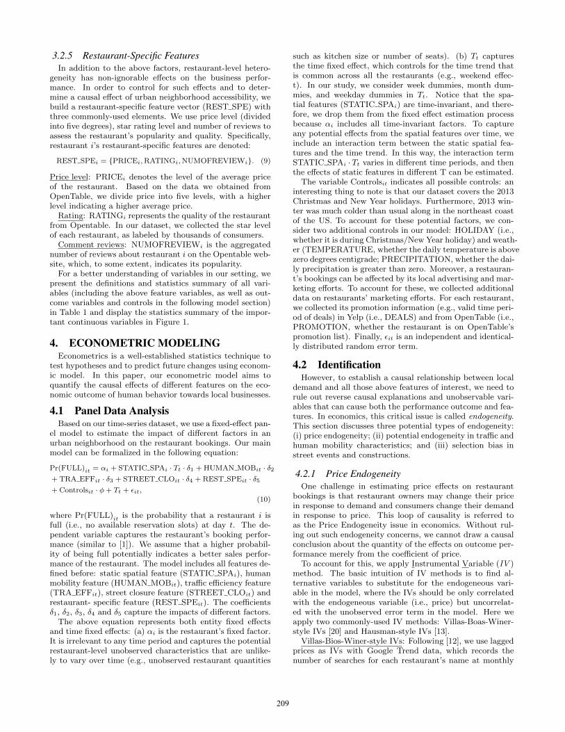
Figure 2: Framework of exploring causal treatmenteffects using Difference-in-Difference method

ner chooses a particular street to closefor a local event orfor construction may be due to some unobserved functionalinability of that street (e.g., poor street condition, locationalinconvenience). Such unobserved factors may cause both thedecision of street closure and the decrease in sales for local s-tores, regardless of the street closure. To account for such anendogeneity issue and to identify the impact from a causalperspective, we conduct an additional analysis by combin-ing Propensity Score Matching (PSM ) and Difference-in-Difference (DID) methods to examine the causal effect ofstreet closure. We illustrate the basic intuition of our anal-ysis design in Figure 2.

First, we consider a four-week time window as the exper-iment period and divide it into two time periods: the first14 days are the baseline period, while the latter 14 days arethe test period. In the baseline period, no street closure(i.e., events or construction) occurs within a 0.5-mile rangeof all the restaurants. In the test period, some restaurantsexperience street closure within the same area1. Second, wedivide restaurants into two groups: a Treatment group inwhich the restaurants have at least one nearby street clo-sure in the test period; and a Control group in which therestaurants remain unaffected in the overall four-week timewindow. Third, to address the issue of selection bias instreet closure, we use Propensity Score Matching (PSM ) forthe counterfactual analysis. The idea of PSM is to matchrestaurants in the Treatment group with those in the Con-trol group based on their likelihood (i.e., propensity score) ofbeing treated. The matching process would help eliminatethe concern that some other observed restaurant character-istics would potentially lead to both the treatment decisionand the observed outcome. Specifically, a logit regression isused to estimate the propensity score for each restaurant:

P (Dit = 1|Vit) =1

1 + exp((−logitit), (11)

where

logitit = αi + STATIC SPAi · Tt · δ1 + HUMAN MOBit · δ2+ TRA EFFit · δ3 + STREET CLOit · δ4 + REST SPEit · δ5 + εit.

(12)

In the Logit regression function, the propensity score P (Dit =1|Vit)indicates the likelihood of the restaurant being select-ed in the treatment group. Vit represents the observable1We selected the time period with the largest number of treatedsamples: from Dec 24, 2013 to Jan 20, 2014. We filtered the wholesample to make the resulting samples satisfy the requirements ofperiod division. To account for the potential bias introduced bythe time period selection, we tested different starting times or dif-ferent lengths of time window. The results stay highly consistent.

feature vectors (i.e., static special features, human mobili-ty features, traffic efficiency features, street closure featuresand restaurant specific features) of restaurant i at time t.In the matching process, we use the K-nearest neighbor al-gorithm. Specifically, the optimal matched pairs of treatedand control observations are those that produce the min-imum distance in their propensity scores. Therefore, therestaurants in a matched pair share a similar possibility ofbeing selected for treatment (i.e., street closure). Howev-er, the only difference between a matched pair is that oneis being treated and the other is not, which nicely simu-lates a randomized control experimental setting. Note thatPSM is particularly appropriate in our case because (1) wehave a large number of sample observations, and (2) we areable to incorporate a large variety of observed time-varyingand time-invariant restaurant-level characteristics into thematching process. Both advantages allow us to identify pairsof restaurants with high similarity.

Finally, based on the matched samples, we use the Difference-in-Difference (DID) method to test the causality. To en-sure that there are no unobserved differences related to thetreatment (i.e., the quality may differ even within the t-wo matched samples due to unobservables), we apply DIDto exploit the exogenous variance in street closure acrossrestaurants and time as the basis for identifying causal ef-fects on local restaurant sales. Our model is as follows,

Pr(FULL)it = αi + β1Testt + β2Testt × Treati+ Controlsit · φ+ Tt + εit.

(13)

where αi is restaurant-level fixed effect; Testt indicates thetest (t = 1) or baseline (t = 0) period; and Treati indicateswhether restaurant i is in the treatment group. Note that,similar to the main estimation, we add additional controlvariables, such as weather, holiday indicator, etc. The coef-ficient of interest is β2, which captures the effects of streetclosure in the test period.

5. RESULTS

5.1 Panel Data Model ResultsWe first start with our main estimation model (Equation

7), the main coefficients of which are shown in Table 2.We allow interactions between static spatial features andtime trend indicators to capture the impacts of static fea-tures over time. Specifically, we define four monthly indica-tors: November and December jointly (m1)2, January (m2),February (m3) and March (m4). To avoid collinearity, weuse only the first three indicators in the regression.

With regard to restaurant-specific features, consistent withtheories3, we find that price has a negative effect on restau-rant bookings and that the effect of price is significantlylarger than that of the other features. The number of re-views presents a significant and positive effect. In addition,our results also show that warm, sunny weather has a sig-nificant and positive effect on local restaurants. This is con-sistent with previous studies that use weather or climate as

2Our data contain two days from November 2013, so we mergethem into the December month dummy.3Rating effect is not statistically significant. We notice that morethan 75% of restaurants have a star rating higher than or equal to3.9, showing a relative small variance. Due to the potential infla-tion of the numerical ratings, it may result in the non-significantcoefficient. But we do observe that this effect is positive.

211

Table 2: Main Estimation ResultsVariable Coef. Variable Coef.Mobility density 0.004** Heterogeneity 0.008

(0.002) ×m1 (0.008)Social stability -0.001 Competitive -0.001

(0.002) ×m1 (0.004)Incoming 0.003 Location -0.001mobility (0.002) density×m2 (0.004)Traffic efficiency -0.005*** Population 0.005***

(0.001) ×m2 (0.001)Street Closure -0.014*** Heterogeneity 0.008

(0.004) ×m2 (0.008)Price -0.034** Competitive -0.053*

(0.001) ×m2 (0.021)Rating 0.002 Location 0.000

(0.004) density×m2 (0.003)Reviews 0.013*** Population 0.001

(0.002) ×m3 (0.001)Location density 0.002 Heterogeneity 0.009×m1 (0.004) ×m3 (0.008)Population 0.011*** Competitive -0.031×m2 (0.001) ×m3 (0.021)

Controls: promotion, temperature, precipitation, and Googletrends; Methods: entity and time fixed effects; Data: 0.5-mileneighborhoods in NYC. Standard erros are shown in parentheses.* p-value<0.05 **p-value<0.01 ***p-value<0.0001

one measure of an urban system [6]. However, our findingmakes a further step to quantify the economic value of thisfactor. Regarding the interactions between static spatialfeatures and time trend (i.e., location density, populationdensity, heterogeneity and competitiveness with month in-dicators m1, m2, m3), we find that most of them do nothave significant impacts, suggesting that most effects fromthe static spatial features are time-invariant and absorbedby the fixed effect. The above results are based on lag-terminstrument variables. We also use our alternative instru-ment variables and obtain the similar results. The resultsin Figure 3 illustrate effects from all time-varying variables:mobility density, social stability, incoming mobility, trafficefficiency, street closure, price comment reviews and ratings.

Figure 3: Comparison of effects between half-milerange and one-mile range neighborhoods.

5.2 PSM and DID Model ResultsTo deal with the potential selection bias in street clo-

sure, we combine the PSM and DID methods to explore thecausal effects. Column (i) in Table 3 shows the coefficientsfrom our causal estimation. The coefficient of “Test” is posi-

Table 3: PSM and DID Model ResultsVariables (i) (ii) (iii).Test × Treat – – -0.047*× NumProj (0.024)Test × Treat -0.074*** -0.018* -0.058***

(0.018) (0.007) (0.019)Test 0.066*** 0.024 0.067***

(0.018) (0.018) (0.011)Promotion control Yes Yes YesWeather control Yes Yes YesTime control Yes Yes YesObservations 11,424 11,144 11,424

(i)&(iii): 12/24/2013-1/20/2014(ii): 11/29/2013-12/26/2013

* p-value<0.05 **p-value<0.01 ***p-value<0.0001Standard erros are shown in parentheses.

tive, indicating that, on average, the baseline booking trendis increasing during this test time period. This is reasonablebecause it is the holiday season, when more consumption islikely to occur. Interestingly, we find a significant and neg-ative sign of the interaction term “Test×Treat”, suggestinga negative causal effect of street closure on bookings. Onemight argue that the time period we cover is special becauseit might cover some unobservable related to the holiday. Tobetter assess our model and results, we conduct robustnesstests on several alternative periods before and after this hol-iday season. We find that the interaction term still shows asignificant negative sign, whereas the baseline time trend isnot significant. Column (ii) shows the results from one alter-native period. Furthermore, to measure the treatment effectat different levels of street closure, we add another interac-tion term, Test × Treat × NumProj (the number of nearbystreet events/constructions). The corresponding model isdescribed in eq. (14). The result is shown in Column (iii).We find results consistent with our main model. Moreover,coefficient δ6 is negative and significant, suggesting that onemore street event nearby leads to a 4.7% decrease in theprobability of a restaurant being fully booked.

Pr(Full)it = αi + β1Testt + β2NumProjit + β3Testt × Treati

+ β4Testt ×NumProjit + β5Treati ×NumProjit+ β6Testt × Treati ×NumProjit + Controlsit · φ+ Tt + εit

(14)

5.3 Additional Robustness TestsTo assess the robustness of features, model and results,

we conduct four additional robustness tests:Robustness Test I: Use the same variables on alterna-

tive models: The dependent variable is discrete coveringsix probability numbers. In this sense, the linear regressionmodel may not fit the data very well. We tried differentmodels, such as logit. In this alternative model, we considerthe dummy dependent variable as the indicator of whetherthe reservation is available at 7pm, which we believe is themost common time that NYC residents go out for dinner.We find similar results with the main estimation.

Robustness Test II: Replace fixed effects with random ef-fects: In our main model, we combine spatial features withtime trend to see impacts over time because the entity-fixed-effects method omits all time-invariant and individual levelfeatures. To test the effectiveness of these static featuresdirectly, we test the random effects model and find similar

212

results. By using the Hausman test, we find that our fixedeffects model performs better.

Robustness Test III: Use detailed traffic information: Toextract the detailed dynamic traffic conditions, we apply thekeyword-extraction technique to classify tweets into differenttypes, based on their keywords: traffic accidents, heavy traf-fic jams, bus delays, etc. That is, we divide the TRA EFFinto six sub variables: ACCIDENT, DISABLED, DELAYS,HEAVYTRAFFIC, WEATHER and EVENTS (the detaileddefinitions are provided in Table 1).We find very similartrends for all factors. In particular, we find a significantnegative effect of bus delays on business performance. Oneexplanation is that our dataset was collected in NYC wherepublic transportation is a major choice, especially duringrush hour (dinner time).

Robustness Test IV: Use alternative range of neighbor-hood on the same model: To examine whether a 0.5-milerange is a valid definition of neighborhood and whether theneighborhood size matters a lot in our estimation, we con-sider neighborhoods of different sizes. The result, shown inFigure 3, is the impact of each factor is similar to that of the0.5-mile range, while the mobile density and dynamic trafficfeatures show larger impacts.

5.4 Interaction Effects ResultsIn the previous process, we considered the 3,187 restau-

rants as a single group, which might lead to some bias be-cause of heterogeneity at the restaurant level. In this subsec-tion, we will look into smaller restaurant groups and examinethe interaction effects of those features of interest.

Interaction Model I: Interaction effects with price levelindicator: First, to explore how effects of traffic efficiencyfeature and the street closure feature vary with price level,we divide the restaurants into two groups: expensive restau-rants and cheap restaurants. Then we add two interactionterms between price dummies (denoting whether or not theprice is high) and the two traffic-related features: traffic ef-ficiency feature and street closure feature. We hold otherthings constant, as in eq. (10). The results show that thecoefficients of the interaction terms are significantly nega-tive, indicating that higher priced restaurants are more liketo be affected by traffic conditions. Figure 4 illustrates thecoefficients of each feature within each group.

Figure 4: Comparison of interaction effects betweentraffic-related features and price levels

Interaction Model II: Interaction effects with chain or in-dependent restaurants indicator: Next, in order to examinewhether the brands have any impacts under this scenario,we divided the 3,187 restaurants into three groups: chainrestaurants, independent restaurants and others. Amongthem, there are 86 well-established chain restaurants with 15brands and 2,354 independent restaurants. By using inter-

action terms combining the chain dummy (denoting whetherit is a chain restaurant) with the traffic efficiency feature andstreet closure feature, we run a fixed-effect regression overthe 2,440 restaurants. The coefficients are both positive,while only the coefficient of the interaction term betweenthe chain dummy and traffic efficiency feature is significant.It implies that chain restaurants will be affected more thanindependent restaurants by unexpected traffic conditions.Figure 5 illustrates such differences.

Figure 5: Comparison of interaction effects betweentraffic-related features and chain/independent indi-cator with 2,440 restaurants

Furthermore, we apply the above division to the PSMand DID estimation procedure to explore whether differentrestaurants (e.g., chain and individual) would be affected bystreet conditions differently:

Pr(FULL)it = αi + β1Testt + β2Testt × Treati

+ β3Testt × Treati × chaini + Controlsit · φ+ Tt + εit,(15)

where chaini is a dummy variable. Again, the lower-orderinteraction term chaini is excluded because it is collinearwith the fixed effects. The results show that both β2 (=−0.053) and β3 (= −0.4214) are significant and negative,suggesting that chain restaurants tend to be affected morethan independent restaurants by road closures.

Interestingly, our findings from this interaction model seemto suggest that chain restaurants are likely to be much morenegatively affected by the street closures when comparedto independent restaurants. This is reasonable because forchain restaurants, when one location becomes less accessi-ble customers who really like the food tend to substituteaway to an alternative location with easy access for thesame chain restaurants. However, for independent restau-rants customers who really like the food do not have an easyalternative for substitution. As a result, they may have amuch higher switching cost compared to the case of chainrestaurants, which might help keep independent restaurantsfrom losing customers. Our results have potential in helpingfranchised restaurant chains to better understand the effect-s of city events and street closures, and to improve theirmarketing strategies to reduce the potential economic loss.

6. DISCUSSION AND FUTURE WORKIn this paper, we explore to the economic values in the ur-

ban system based on geotagged and crowdsourced data fromvarious large-scale social media sites and publicly availabledata sources. Using geo-mapping and geo-social-taggingtechniques, together with natural language processing, weidentify four feature dimensions to describe the potentialsocial and economic factors of local demand. After evalu-ating these features while also accounting for the potential

213

endogeneity issues, our econometric model is able to quan-tify the economic and social value of the extracted featureson local demand from a causal perspective.

On a broader note, the objective of this paper is to illus-trate how multiple and diverse sources of publicly availablecrowdsourced data can be mined and incorporated into theprediction of local demand to enhance the understanding ofusers’ economic behavior through its interactions with localbusinesses. Our study demonstrates the potential of how wecan best make use of the large volumes of user-generatedcontent and geotagged social media data to create matricesthat capture multidimensional characteristics in a mannerthat is fast, cheap, accurate, and meaningful. Local busi-nesses can use this information to proactively design theirbusiness strategies (e.g., advertising and promotions) whenfacing a potential change of its neighborhood city services.Furthermore, it can help government decision makers to un-derstand local economic trends. For example, it is useful forurban planners to be able to quantify the opportunity cost,and moreover, the overall expected economic outcome of anurban project or event in a location, under various urbanand economic conditions. Since our data come from publiclyavailable channels, we can easily apply our methodology toother categories of local businesses in various locations. Suchanalyses can help small businesses gain insights into their lo-cal urban systems and economies, which, in turn, increasestheir success and the sustainability of urban neighborhoods.

Our research also has implications for location-based ser-vices, such as Google Maps, by making it possible to incor-porate data into understanding local neighborhoods. Specif-ically, they can use the model we propose to specify the lo-cation efficiency scores in predicting the economic potentialfor a new market. For example, one possibility would be toprovide an “economic index” of each neighborhood for newbusinesses to predict their demand in different locations and,thus, optimize their location selection.

Our work has several limitations, some of which can serveas fruitful areas for future research. Our analysis is based ona randomly selected subset of Twitter and Foursquare da-ta. It can be improved by leveraging more data from othercrowdsourced channels to gain a more comprehensive under-standing of traffic and human mobility conditions. Also, inorder to better predict the local demand, future work canlook into not only the geographic and socioeconomic per-spectives of cities, but also other natural and environmentalaspects, such as climate and pollution factors, healthcare,etc. Such research would help us draw a comprehensive pic-ture of the overall urban system and to study the economicdynamics and social interactions more precisely.

7. REFERENCES[1] M. Anderson and J. Magruder. Learning from the

crowd: Regression discontinuity estimates of theeffects of an online review database*. The EconomicJournal, 122(563):957–989, 2012.

[2] G. C. Blomquist, M. C. Berger, and J. P. Hoehn. Newestimates of quality of life in urban areas. TheAmerican Economic Review, pages 89–107, 1988.

[3] BusinessWeek. It costs $333 million to shut downboston for a day. 2013a.www.businessweek.com/articles/2013-04-19/

it-costs-333-million-to-shut-down-boston-for-a-day.

[4] P. Calthorpe. The next American metropolis: Ecology,community, and the American dream. PrincetonArchitectural Press, 1993.

[5] Z. Cheng, J. Caverlee, K. Lee, and D. Z. Sui.Exploring millions of footprints in location sharingservices. ICWSM, 2011:81–88, 2011.

[6] P. C. Cheshire and S. Magrini. Population growth ineuropean cities: weather matters–but only nationally.Regional studies, 40(1):23–37, 2006.

[7] J. A. Chevalier and D. Mayzlin. The effect of word ofmouth on sales: Online book reviews. Journal ofmarketing research, 43(3):345–354, 2006.

[8] E. Cho, S. A. Myers, and J. Leskovec. Friendship andmobility: user movement in location-based socialnetworks. In Proceedings of the 17th ACM SIGKDD,pages 1082–1090. ACM, 2011.

[9] R. Ewing and S. Handy. Measuring the unmeasurable:urban design qualities related to walkability. Journalof Urban design, 14(1):65–84, 2009.

[10] R. Florida. The economic geography of talent. Annalsof the Association of American geographers,92(4):743–755, 2002.

[11] C. Forman, A. Goldfarb, and S. Greenstein. How didlocation affect adoption of the commercial internet?global village vs. urban leadership. Journal of urbanEconomics, 58(3):389–420, 2005.

[12] A. Ghose, P. G. Ipeirotis, and B. Li. Designingranking systems for hotels on travel search engines bymining user-generated and crowdsourced content.Marketing Science, 31(3):493–520, 2012.

[13] J. A. Hausman. Valuation of new goods under perfectand imperfect competition. In The economics of newgoods, pages 207–248. 1996.

[14] D. Karamshuk, A. Noulas, S. Scellato, V. Nicosia, andC. Mascolo. Geo-spotting: Mining onlinelocation-based services for optimal retail storeplacement. In Proceedings of the 19th ACM SIGKDD,pages 793–801. ACM, 2013.

[15] D. Lambiri, B. Biagi, and V. Royuela. Quality of lifein the economic and urban economic literature. SocialIndicators Research, 84(1):1–25, 2007.

[16] J. Lindqvist, J. Cranshaw, J. Wiese, J. Hong, andJ. Zimmerman. I’m the mayor of my house: examiningwhy people use foursquare-a social-driven locationsharing application. In Proceedings of the SIGCHIConference on Human Factors in Computing Systems,pages 2409–2418. ACM, 2011.

[17] T. Litman. Economic value of walkability.Transportation Research Record: Journal of theTransportation Research Board, (1828):3–11, 2003.

[18] X. Lu, S. Ba, L. Huang, and Y. Feng. Promotionalmarketing or word-of-mouth? evidence from onlinerestaurant reviews. Information Systems Research,24(3):596–612, 2013.

[19] T. Sakaki, M. Okazaki, and Y. Matsuo. Earthquakeshakes twitter users: real-time event detection bysocial sensors. In Proceedings of the 19th internationalconference on World wide web, pages 851–860, 2010.

[20] J. M. Villas-Boas and R. S. Winer. Endogeneity inbrand choice models. Management Science,45(10):1324–1338, 1999.

214