Understanding Typological Distributions II · 2. Measuring variation in p-domains ... (17) Bickel, Hildebrandt, & Schiering, ... Dutch French (colloquial) Garo Greek (modern) Hayu

Understanding Typological

Distributions II

Balthasar Bickel

U. Leipzig

Wrapping up and going on

•In the phonological words example, we saw that languages tend to have many distinct p-words

•One approach to analyze them is to take each p-word as a datapoint of its own and then analyze the distribution of these datapoints in the world seeking non-accidental skewings.

•A hypothesis: since stress patterns systematically interact with higher-level domains (phrases, utterances; information structure), they target larger domains.

2

Measuring variation in p-domains

• Hypothesized to be very common:Limbu (Sino-Tibetan) Stress: [prefix-'stem-suffix=clitic][mɛ-'thaŋ-e=aŋ] 3ns-come.up-PST=and

• Hypothesized to be much less common:Mon (Austroasiatic) Stress: ['cl]=[pf<infix>'stem]=['cl][k<ə>'lɒʔ] <CAUS>cross ['kɒ]=['klɒʔ] CAUS=cross

3 Bickel, Hildebrandt, & Schiering, in press.


•To test this hypothesis, we need a measure of relative size, ‘coherence’:

4

c(p; L) = N (morpheme types referenced by p)N (morpheme types in L)

Bickel, Hildebrandt, & Schiering, in press.

Bickel, Hildebrandt, & Schiering, in press.


5

morpheme types in domain

available morpheme types

De

nsit

y o

f p

ho

no

log

ica

l p

att

ern

s

0

1

2

3

assimilation constraint deletion insertion

0

1

2

3

quantity size_related strengthening stress

0

1

2

3

0.0 0.5 1.0 1.5

tone

0.0 0.5 1.0 1.5

vowel_harmony

0.0 0.5 1.0 1.5

weakening

Testing statistical universals: two key problems

1.The INFERENCE problem: how to extrapolate from a sample to all human languages in the absence of random sampling? (NB: there already have been at least 500,000 languages, but we know only about 500!)

2.The DIACHRONY problem: how to tell apart the factors determing the observed cross-linguistic distribution?

•Structural Pressure (‘what works best, replicates best’; a.k.a. ‘selection’, ‘functional pressure’, ‘preferred pathways of change’, ‘linguistic principles’)

•Language Contact (‘what is most popular, replicates best’)

•Blind Inheritance (‘what was best for our parents, is best for us’)

•Random fluctuation

6

Toward a solution

•If we can solve the Diachrony Problem, we have solved the Inference Problem:

•if we know that a distribution is due to Structural Pressure, independent of any other diachronic factor, this Structural Pressure determines how languages develop over time, beyond what we can observe now.

7

Solving the Diachrony Problem

•Useful reformulation of empirical universals: instead of p → q,

•E(q) ~ p,

•where E represent the expected mean of q, given p

•E(q) can be directly linked to p if q is continuous; nominal q need to be transformed first by what is called a ‘link function’ g(), usually the natural logarithm of odds (‘logit’, ‘logistic regression’) or counts (‘loglinear analysis’). This defines the Generalized Linear Model:

g(E(q)) = α + β1p1 + β2p2 ... + βkpk

• bidirectional universals have an additional condition: odds(q) ≠ 1 under any level of p.

• unrestricted universal: g(E(q)) = α, and α deviates from H0.

8

Using Generalized Linear Models for testing universals

•p can be on any scale. If it is binomial, β represents the difference in q between p=0 (e.g. OV) and p=1 (e.g. VO). All multinomial p with k levels can be ‘parametrized’ into k-1 paramaters (a.k.a. ‘dummy variables)

•Note that p can be a complex vector of predictors (‘competing motivations’), including also linguistic areas!

•And it can include interactions pipj, i.e. differences in effects between levels of pi across levels of pj.

•The goal of statistical analysis is to find those coefficients that best describe the data (e.g. via Least Squares or Maximum Likelihood Estimation) and then to test whether these coefficients are significantly different from zero, i.e. ‘belong to the model’.

9

Solving the Diachrony Problem

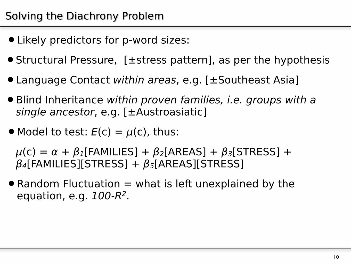
•Likely predictors for p-word sizes:

•Structural Pressure, [±stress pattern], as per the hypothesis

•Language Contact within areas, e.g. [±Southeast Asia]

•Blind Inheritance within proven families, i.e. groups with a single ancestor, e.g. [±Austroasiatic]

•Model to test: E(c) = µ(c), thus:

µ(c) = α + β1[FAMILIES] + β2[AREAS] + β3[STRESS] + β4[FAMILIES][STRESS] + β5[AREAS][STRESS]

•Random Fluctuation = what is left unexplained by the equation, e.g. 100-R2.

10

Plausible areal factors in phonological domains

Southeast Asia (Matisoff 2001, Enfield 2005), South- Southwest Asia (Masica 1976, 2001, Ebert 2001); Europe (Dahl 1990, Haspelmath 2001, Heine & Kuteva 2006)

11Bickel, Hildebrandt, & Schiering, in press

SSWA

SEA

SEA

SEA

SEA

EU

EU

SSWA

EU

SSWA

EU

SEA

SEA

SSWA

SSWA

SSWA

SEA

SSWA

SSWA

EU

SSWA

SEA

SEA

SEA

SSWASSWA

SEA

SSWA

EU

SEA

EU

SSWA

SEA

EU

EU

SEA

SSWA

SEA

Armenian (Eastern)

Burmese

Cambodian

Cantonese

Chrau

Dutch

French (colloquial)

Garo

Greek (modern)

Hayu

Irish

Jahai

Kayah Li (Red Karen)

Kham

Kharia

Khasi

Khmu

Kinnauri

Limbu

Lithuanian

Manange

Mandarin

Meithei (Manipuri)

Mon

NepaliNewar (Dolakha)

Pacoh

Persian

Polish

Qiang

Romani (Sepecides)

Santali

Semelai

Spanish

Swedish

Tibetan (Dege)

Tibetan (Kyirong)

Wu

SSWA

SSWA

SSWA

SSWA

SSWA

SSWA

SSWA

SEA

SSWA

SSWA

SSWA

SSWA

Garo

Hayu

Kham

Kharia

Khasi

Limbu

Manange

Meithei (Manipuri)

Nepali

Newar (Dolakha)

Santali

Tibetan (Kyirong)

Plausible family factors in phonological domains

The chosen areas allow similarly-sized family samples, with one representative per sub-branch of major branches in three families (or two if phonologies are known to be diverse and data are sufficient): Austroasiatic (11), Indo-European (12), Sino-Tibetan (17)


IE

ST

AA

ST

AA

IE

IE

ST

IE

ST

IE

AA

ST

ST

AA

AA

AA

ST

ST

IE

ST

ST

ST

AA

IEST

AA

IE

IE

ST

IE

AA

AA

IE

IE

ST

ST

ST

Armenian (Eastern)

Burmese

Cambodian

Cantonese

Chrau

Dutch

French (colloquial)

Garo

Greek (modern)

Hayu

Irish

Jahai

Kayah Li (Red Karen)

Kham

Kharia

Khasi

Khmu

Kinnauri

Limbu

Lithuanian

Manange

Mandarin

Meithei (Manipuri)

Mon

NepaliNewar (Dolakha)

Pacoh

Persian

Polish

Qiang

Romani (Sepecides)

Santali

Semelai

Spanish

Swedish

Tibetan (Dege)

Tibetan (Kyirong)

Wu

ST

ST

ST

AA

AA

ST

ST

ST

IE

ST

AA

ST

Garo

Hayu

Kham

Kharia

Khasi

Limbu

Manange

Meithei (Manipuri)

Nepali

Newar (Dolakha)

Santali

Tibetan (Kyirong)

Model testing

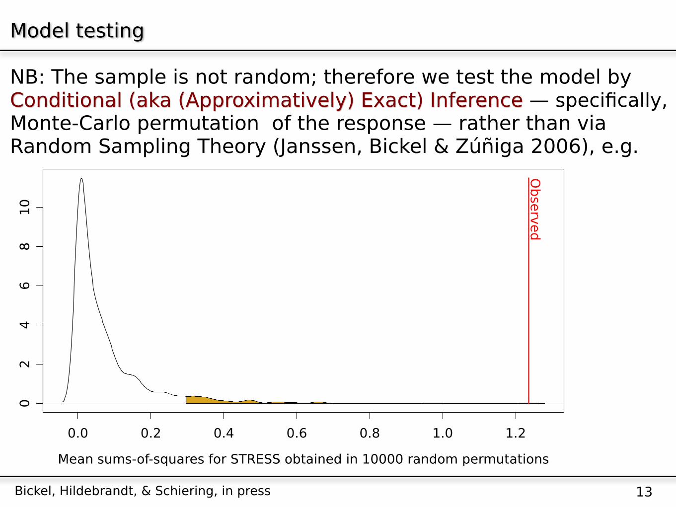
NB: The sample is not random; therefore we test the model by Conditional (aka (Approximatively) Exact) Inference — specifically, Monte-Carlo permutation of the response — rather than via Random Sampling Theory (Janssen, Bickel & Zúñiga 2006), e.g.


0.0 0.2 0.4 0.6 0.8 1.0 1.2

02

46

810

Mean sums-of-squares for STRESS obtained in 10000 random permutations

Densit

y

Observ

ed

Model testing

Based on 238 sound patterns in 40 languages, we find:

•no evidence for any interactions between any factors;

•no evidence for an AREA effect (F(2)=.92, p=.51)

a significant main effect of STOCK (F(2)=11.03, p<.001)

•a significant main effect of PATTERN TYPE (F(1)=20.99, p<.001)


Model testing

The best-fitting model is μ(c) = .69 - .30[IE vs AA] - 1.4 [ST vs AA] + .26 [STRESS vs OTHER]

15

morp

hem

e t

ypes in d

om

ain

available

morp

hem

e t

ypes

0.2

0.4

0.6

0.8

1.0

Austroasiatic Indo-European Sino-Tibetan

other

Austroasiatic Indo-European Sino-Tibetan

stress-related

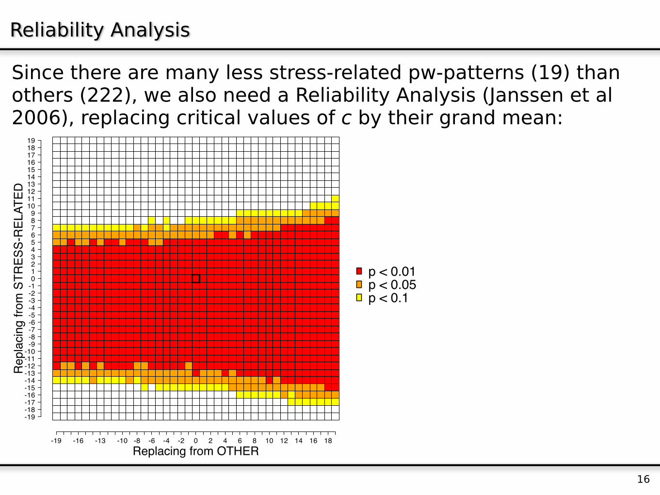
Since there are many less stress-related pw-patterns (19) than others (222), we also need a Reliability Analysis (Janssen et al 2006), replacing critical values of c by their grand mean:

Reliability Analysis

16Replacing from OTHER

Repla

cin

g fro

m S

TR

ES

S-R

ELA

TE

D

-19 -4 7 19

-19-18-17-16-15-14-13-12-11-10-9-8-7-6-5-4-3-2-10123456789

10111213141516171819 p < 0.01p < 0.05p < 0.1

Replacing from OTHER

Repla

cin

g fro

m S

TR

ES

S-R

ELA

TE

D

-19 -16 -13 -10 -8 -6 -4 -2 0 2 4 6 8 10 12 14 16 18

-19-18-17-16-15-14-13-12-11-10

-9-8-7-6-5-4-3-2-10123456789

10111213141516171819 p < 0.01

p < 0.05

p < 0.1

Interim conclusions

•There is evidence for structural pressure leading to phonologies in which stress domains are larger than other domains.

•There are no other statistical signals, i.e. no other type of phonological pattern seems to favor a specific domain size.

•No evidence for hierarchical nesting anywhere

•The universal is independent of the effects from language contact (areas) and blind inheritance (families), but

•blind inheritance also (independently) matters — but without interaction!

•This is in line with known diachronic preferences for structure preservation (Blevins 2004)

17

Prospects for larger datasets

•But... how can extend the test to a worldwide database?

•Including the stock factor into regression models makes no sense in worldwide datasets because there are over 300 stocks...

•Need a completely new approach!

18

Towards a new approach

•Two observations:

1.Distributions of linguistic structures change over time.

2.Changes over time are described by reconstructed families (by which I exclusively mean units demonstrated by the comparative method).

•Therefore, any universal can be understood as universal pressure for families to develop a specific skewing, as they split over time (Greenberg 1978, 1995, Maslova 2000, Nichols 2003, etc.).

19

Towards a new approach

•Therefore, all universals are in fact diachronic in nature!

•We can reformulate every universal as diachronic pressure, e.g. “VO → NRel” can be reformulated as:π(VO&RelN ↣ VO&NRel) > π(VO&NRel ↣ VO&RelN), where “↣” symbolizes diachronic change

•Given this, ‘diachronic universals’ are just a special case, concerning the explanation of the universal“OV → Np”: π(OV&pN ↣ OV&Np) > π(OV&Np ↣ OV&pN) because NOV frequently develops into Np (e.g. Nepali ājā bhane ‘today (NO) saying (V)’ > ‘as for (P) today (N)’)

20

Towards a new approach: the Skewed Family Method

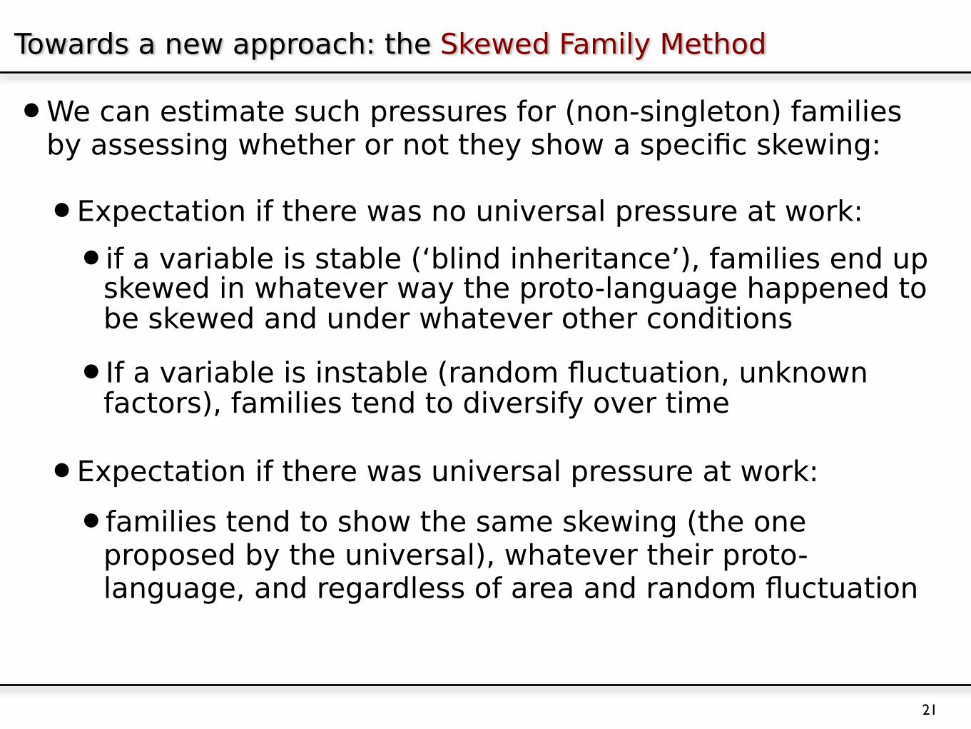
•We can estimate such pressures for (non-singleton) families by assessing whether or not they show a specific skewing:

•Expectation if there was no universal pressure at work:

•if a variable is stable (‘blind inheritance’), families end up skewed in whatever way the proto-language happened to be skewed and under whatever other conditions

•If a variable is instable (random fluctuation, unknown factors), families tend to diversify over time

•Expectation if there was universal pressure at work:

•families tend to show the same skewing (the one proposed by the universal), whatever their proto-language, and regardless of area and random fluctuation

21

Towards a new approach: the Skewed Family Method

•Therefore, if most (according to some statistical test) families are skewed in the same way regardless of their areal locations and regardless of any structural condition, this attests to universal pressure.

•To what extent is this a valid inference?

22

Informal Proof

• Given universal family skewing in a distribution D, assume this to result from blind inheritance within each family.→ The current D(G0) reflects D(G-1).→ Unless there was universal pressure before G-1, all D(Gk)

must reflect D(Gk-1) until k spans the entire history of the human language faculty.

→ D must be super-stable over deep time.→ Changes in D are extremely unlikely within short time

intervals.• Assume that all reconstructible time intervals are short (up to

about 8Ky, the age of provable families)→ Expect to be able to observe almost no changes in D.→ Almost all observable families must be uniform.

• Conclusion: unless this is the reality, it is safe to reject blind inheritance as a cause of universal family skewing.

23

Estimates on plausible stability

•What is the highest plausible probability of random change (A→B, B→A) such that

•given a significant skewing of a binary variable {A,B} in an observable sample size of 1000 languages (e.g. 40% vs 60%, or 10% vs. 90%),

•the skewing is still detectable after at least 100 generations of languages (i.e. about 100Ky of history), and

•the expected numbers of observable changes is significantly smaller than what one observes?

24

Estimates on plausible probabilities of random change prc

• Assume 130 non-singleton documented families: the largest available database (Dryer 2005 on word order) has 131

• We usually find more than 10 cases of change in 130 families, so prc ≤ .10

• But at prc=.10, the proability of keeping statistical signals is below 5%. Sample simulations:

25

Sample simulations

26

0 20 40 60 80 100

0.5

0.7

0.9

1.1

4:6 signal kept

Generations of change at p!.10

Od

ds (!)

original

final

0 20 40 60 80 100

0.5

0.7

0.9

1.1

4:6 signal lost


Od

ds (!)

original

final

0 20 40 60 80 100

0.2

0.4

0.6

0.8

1.0

1.2

2:8 signal kept


Od

ds (!)

original

final

0 20 40 60 80 100

0.2

0.4

0.6

0.8

1.0

1.2

2:8 signal lost


Od

ds (!)

original

final

Estimates on plausible probabilities of random change prc

•The simulation results suggest that as long as we observe at least a handful of non-uniform families, Blind Inheritance cannot explain family skewing: the probability of finding that many cases just must be much higher than what could keep a distribution stable over many generations.

•This validates the inference from universal family skewing to structural pressure.

27

Algorithm for this: www.uni-leipzig.de/~autotyp/gsample3.r

Example: Greenberg #1 (“A before O preference”)

28

language mbranch aoLealao Chinantec Chinantecan OAChinantec (Comaltepec) Chinantecan AOChinantec (Quiotepec) Chinantecan AOChinantec (Palantla) Chinantecan AOMixtec (Chalcatongo) Mixtecan AOMixtec (Ocotepec) Mixtecan AOMixtec (Peñoles) Mixtecan AOMixtec (Jicaltepec) Mixtecan AOMixtec (Yosondúa) Mixtecan AOTrique (Copala) Mixtecan AOOtomi (Mezquital) Otomian OAOcuilteco Otomian AOChichimec Pamean AOPame Pamean AOIsthmus Zapotec Zapotecan AOChatino (Sierra Occidental) Zapotecan AOChatino (Yaitepec) Zapotecan AOZapotec (Mitla) Zapotecan AO

stock distribution majority.value diversityOtomanguean skewed(trend) AO 10.89

Raw data for Otomanguean

Within-family skewing, based on a permutation-based χ2 test (α=.05)

Data: merged data on the ordering of A and O from Dryer 2005 (WALS) and AUTOTYP, 100% matched coding, total N = 1115, joined to AUTOTYP’s critical (conservative) genealogical taxonomy

Example: Greenberg #1 (A before O preference)

29

•Hypothesis: N (families with A≺O skewing) > N (families with no O≺A skewing or no skewing at all).

•One plausible areal control factor is the Circum-Pacific Macro-Area (on which 40% WALS variables show a statistical signal at an α-level of .05: Bickel & Nichols 2006):

Example: Greenberg #1 (A before O preference)

30

•Results:

•No evidence for CP factor, Fisher Exact p=.09

•Significant preference for A≺O skewing: χ2=86.73, prnd<.001

CP OtherSkewed towards AOSkewed towards OAno skewing in stock

67 (e=69) 39 (e=37)1* (e=1) 0 (e=0)6 (e=4) 0 (e=2)

* Perhaps 0, since the only case is Chumashan, represented why what may have been dialects; i.e. this datapoint might actually represent a singleton stock (Mithun 1999:389)

Another problem

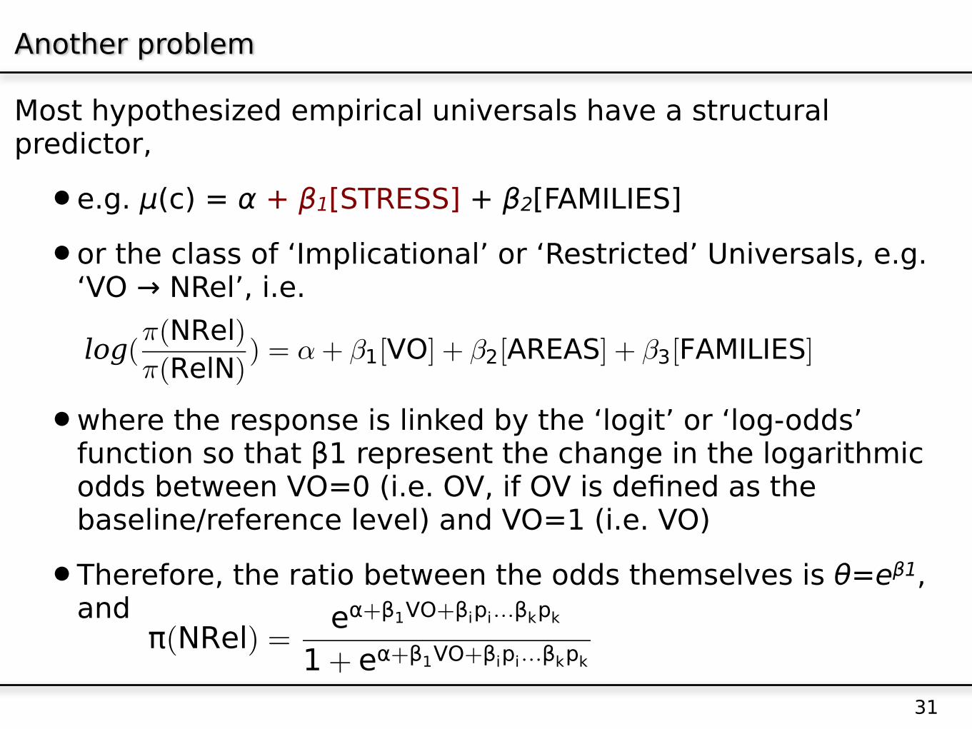
Most hypothesized empirical universals have a structural predictor,

•e.g. µ(c) = α + β1[STRESS] + β2[FAMILIES]

•or the class of ‘Implicational’ or ‘Restricted’ Universals, e.g. ‘VO → NRel’, i.e.

•where the response is linked by the ‘logit’ or ‘log-odds’ function so that β1 represent the change in the logarithmic odds between VO=0 (i.e. OV, if OV is defined as the baseline/reference level) and VO=1 (i.e. VO)

•Therefore, the ratio between the odds themselves is θ=eβ1, and

31

test

log(!(NRel)!(RelN)

) = "+ #1[VO] + #2[AREAS] + #3[FAMILIES](1)

1

log(!(nonneutral)

!(neutral | diverse)) = !19.56+ 3.57FINAL+ !AA+ ....+ !YY

"(NRel) =e#+!1VO+!ipi...!kpk

1+ e#+!1VO+!ipi...!kpk

1

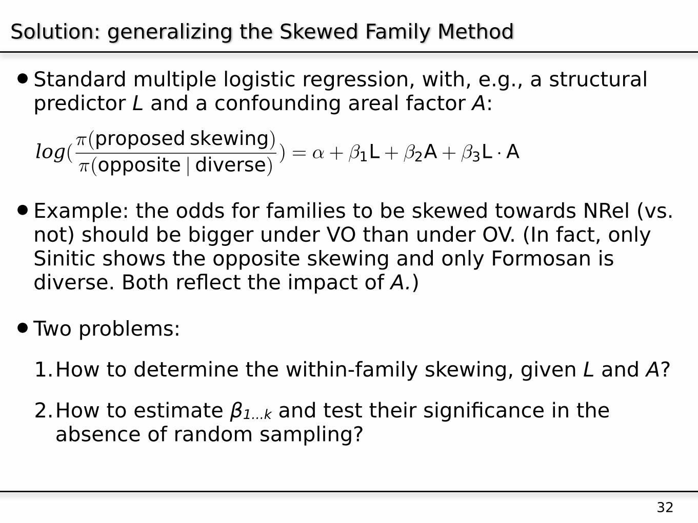
Solution: generalizing the Skewed Family Method

•Standard multiple logistic regression, with, e.g., a structural predictor L and a confounding areal factor A:

•Example: the odds for families to be skewed towards NRel (vs. not) should be bigger under VO than under OV. (In fact, only Sinitic shows the opposite skewing and only Formosan is diverse. Both reflect the impact of A.)

•Two problems:

1.How to determine the within-family skewing, given L and A?

2.How to estimate β1...k and test their significance in the absence of random sampling?

32

test

log(!(proposed skewing)!(opposite | diverse)

) = "+ #1L+ #2A+ #3L · A(1)

1

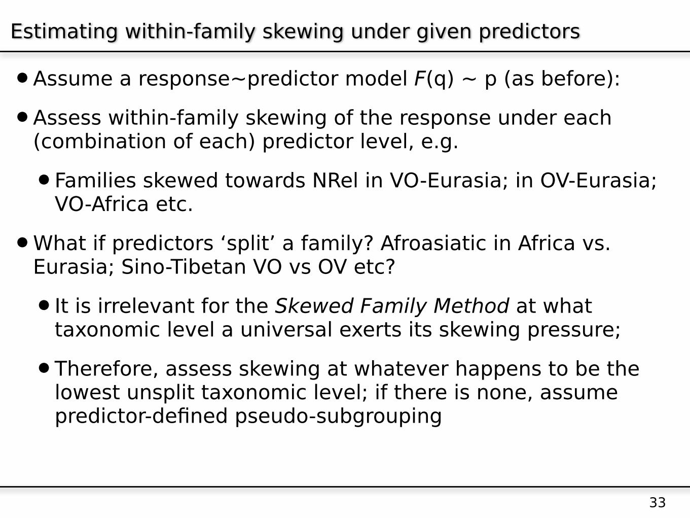
Estimating within-family skewing under given predictors

•Assume a response~predictor model F(q) ~ p (as before):

•Assess within-family skewing of the response under each (combination of each) predictor level, e.g.

•Families skewed towards NRel in VO-Eurasia; in OV-Eurasia; VO-Africa etc.

•What if predictors ‘split’ a family? Afroasiatic in Africa vs. Eurasia; Sino-Tibetan VO vs OV etc?

•It is irrelevant for the Skewed Family Method at what taxonomic level a universal exerts its skewing pressure;

•Therefore, assess skewing at whatever happens to be the lowest unsplit taxonomic level; if there is none, assume predictor-defined pseudo-subgrouping

33

Example: VP order [±VO] as a predictor

•The predictor is split in the WALS database on Sino-Tibetan at the stock level, but not at the major branch level. Therefore estimate skewing at the major branch level:

•Sinitic and Karenic (VO) vs. all other major branches (OV)

•Establish skewing of the response within major branches:

34

unit majority.response distribution VPSinitic (3)Karenic (4)Angami-Pochuri Group (2)Bodic (8)Brahmaputran (4)Kiranti (6)Lolo-Burmese (6)Newaric (2)Remnant Himalayish (2)Tani (3)West Himalayish (2)

RelN skewed(absolute) VONRel skewed(absolute) VOdiverse diverse OVRelN skewed(absolute) OVdiverse diverse OVRelN skewed(absolute) OVRelN skewed(absolute) OVRelN skewed(absolute) OVRelN skewed(absolute) OVRelN skewed(absolute) OVdiverse diverse OV

Example: VP order [±VO] as a predictor

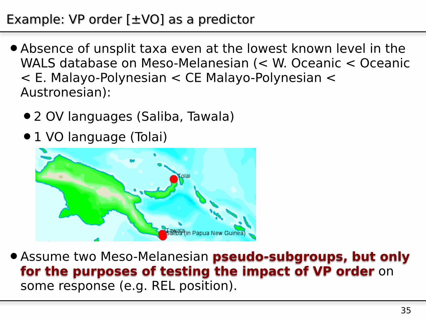
•Absence of unsplit taxa even at the lowest known level in the WALS database on Meso-Melanesian (< W. Oceanic < Oceanic < E. Malayo-Polynesian < CE Malayo-Polynesian < Austronesian):

•2 OV languages (Saliba, Tawala)

•1 VO language (Tolai)

•Assume two Meso-Melanesian pseudo-subgroups, but only for the purposes of testing the impact of VP order on some response (e.g. REL position).

35

Case Study: the distribution of case over word order

•Hawkins 2004: Verb-final languages favor rich case “for reasons of on-line efficiency” (‘rich’ = distinct coding of agent and patient)

•Nichols 1992, Siewierska 2005, Dryer 1989, 2000, Bickel & Nichols 2007: the distribution of both case and word order is heavily affected by areal patterns:

36

Rich case OV vs VO order


•Data on rich case from Comrie 2005 (WALS) and AUTOTYP, 1% mismatches

•Data on word order from Dryer 2005 (WALS) and AUTOTYP, 0% mismatches

•Total datapoints with information on both variables: N = 350

•Stocks with more than one member: N = 51

•Areal confounding factor chosen here for illustration: Eurasia, known to have more case than the rest of the world.(‘neutral’ = no markersdistinguishing A from O)

37

Other Eurasia

non-neutral

neutral

0.0

0.2

0.4

0.6

0.8

1.0


Distribution of case across families (‘trend’: skewing with p<.05):

38

family.name majority.response distribution final EURASIA taxonomic.levelAdamawa-Ubangi neutral skewed(absolute) non_final Other stockArawakan (Maipurean) neutral skewed(absolute) non_final Other stock pseudo-groupArawakan (Maipurean) neutral skewed(absolute) final Other stock pseudo-groupAtlantic neutral skewed(absolute) non_final Other stockAwyu-Dumut neutral skewed(absolute) final Other stockBalto-Slavic non-neutral skewed(absolute) non_final Eurasia mbranchBenue-Congo neutral skewed(trend) non_final Other stockBerber non-neutral skewed(absolute) non_final Other stockCariban neutral skewed(absolute) non_final Other stock pseudo-groupCariban neutral skewed(absolute) final Other stock pseudo-groupCentral (West Semitic) diverse diverse non_final Other sbranchCentral Indo-Aryan non-neutral skewed(absolute) final Other ssbranch pseudo-groupCentral Indo-Aryan non-neutral skewed(absolute) final Eurasia ssbranch pseudo-groupCentral Malayo-Polynesian neutral skewed(absolute) non_final Other sbranchCentral Pacific diverse diverse non_final Other lsbranchCentral Tungusic non-neutral skewed(absolute) final Other mbranchChadic neutral skewed(absolute) non_final Other stockChibchan diverse diverse final Other stockChumashan neutral skewed(absolute) non_final Other stockCushitic non-neutral skewed(absolute) final Other stockDravidian non-neutral skewed(absolute) final Eurasia stockEastern Mon-Khmer neutral skewed(absolute) non_final Eurasia mbranchEskimo-Aleut non-neutral skewed(absolute) final Other stock


39

Pro

port

ion o

f fa

milie

s

skew

ed t

ow

ard

s c

ase

Other Eurasia


•Model to analyze:

•Problem: how to estimate β1...3 and their probability of being ≠ 0, given that the data are not randomly sampled?

•Like before, apply Monte-Carlo permutation tests, i.e. permute the raw response, estimate models by Standard Maximum Likelihood Estimation, and then count how often the Likelihood Ratio (Deviance) is as high as the one in models of the observed data (e.g. Good 1999).

•Or (for smaller datasets): conditional regression by estimating βk in a Markov Chain Monte-Carlo sample set with the same margin totals as those defined by the remaining parameters α and βi, k≠i (Agresti 2002; Forster et al. 2003; Zamar et al. 2007)

40

test

log(!(nonneutral)

!(neutral | diverse)) = "+ #1FINAL+ #2EU+ #3FINAL · EU(1)

1


Results:

•MLE: significant interaction term β3, LR=-4.15, p(X2) =.042

•Monte-Carlo permutation of LR: p = .054 (10,000 re-samples)

•Best-fitting model:

41


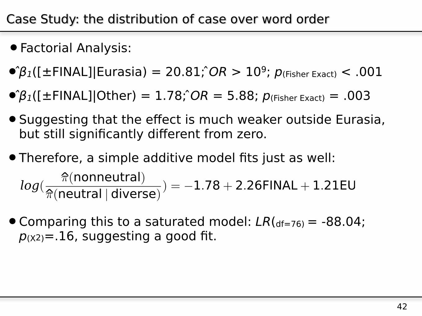
•Factorial Analysis:

• β1([±FINAL]|Eurasia) = 20.81; OR > 109; p(Fisher Exact) < .001

• β1([±FINAL]|Other) = 1.78; OR = 5.88; p(Fisher Exact) = .003

•Suggesting that the effect is much weaker outside Eurasia, but still significantly different from zero.

•Therefore, a simple additive model fits just as well:

•Comparing this to a saturated model: LR(df=76) = -88.04; p(X2)=.16, suggesting a good fit.

42


•Overall OR([±FINAL]) = e2.26 = 9.59

•Overall OR([±EURASIA]) = e1.21 = 3.46

•In words: the odds of families to develop a skewing towards languages with rich case marking are almost 10 times higher if the family has V-final order than if it has non-V-final order; and 3.5 times higher in Eurasia than elsewhere.

43

Pro

port

ion o

f fa

milie

s

skew

ed t

ow

ard

s c

ase

Other Eurasia

An additional benefit of the method

•Since area is modelled as a regression factor, factorial analysis is needed only if there is an interaction.

•If there is no interaction, factorial analysis can be missleading.

•Example: take macro-continents as an areal control, in the spirit of Dryer 1989, 2000:

44

Macrocontinents as areal control factor

Traditional method: test proportions within each area (Fisher Exact Test)

45

Africa p=.45

non_final final

Americas p=.07

non_final final

Eurasia p=.002

non_final final

NG-Australia p=1

non_final final


A better graph (Meyer et al. 2006, package {vcd} in R)

46

Pro

port

ion o

f fa

milie

s

skew

ed t

ow

ard

s c

ase

Africa

p=.45

Americas

p=.07

Eurasia

p=.002

NG-Australia

p=1


•Results from regression analysis:

Best-fitting model:

•FINAL: LR(1)=13.20, p<.001

•MACROCONTINENTS: LR(3)=7.32, p=.07

47

Pro

port

ion o

f fa

milie

s

skew

ed t

ow

ard

s c

ase

Africa Americas Eurasia NG-Australia

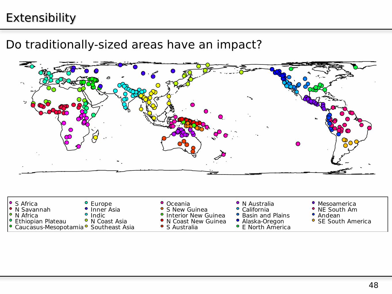
Extensibility

Do traditionally-sized areas have an impact?

48

S AfricaN SavannahN AfricaEthiopian PlateauCaucasus-Mesopotamia

EuropeInner AsiaIndicN Coast AsiaSoutheast Asia

OceaniaS New GuineaInterior New GuineaN Coast New GuineaS Australia

N AustraliaCaliforniaBasin and PlainsAlaska-OregonE North America

MesoamericaNE South AmAndeanSE South America

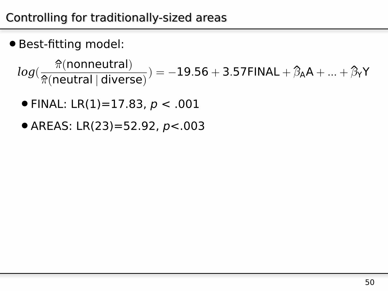
Controlling for traditionally-sized areas

49

Pro

port

ion o

f fa

milie

s

skew

ed t

ow

ard

s c

ase

A B C D E F G H I J K L

Linguistic areas

Pro

port

ion o

f fa

milie

s

skew

ed t

ow

ard

s c

ase

M N O P Q R S T U V W X

Controlling for traditionally-sized areas

•Best-fitting model:

•FINAL: LR(1)=17.83, p < .001

•AREAS: LR(23)=52.92, p<.003

50

Issues of time depth

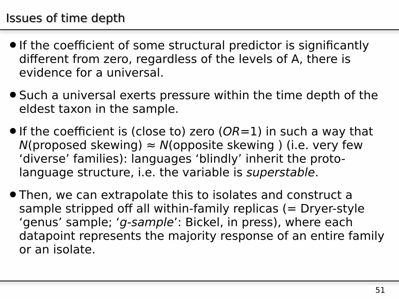
•If the coefficient of some structural predictor is significantly different from zero, regardless of the levels of A, there is evidence for a universal.

•Such a universal exerts pressure within the time depth of the eldest taxon in the sample.

•If the coefficient is (close to) zero (OR=1) in such a way that N(proposed skewing) ≈ N(opposite skewing ) (i.e. very few ‘diverse’ families): languages ‘blindly’ inherit the proto-language structure, i.e. the variable is superstable.

•Then, we can extrapolate this to isolates and construct a sample stripped off all within-family replicas (= Dryer-style ‘genus’ sample; ‘g-sample’: Bickel, in press), where each datapoint represents the majority response of an entire family or an isolate.

51

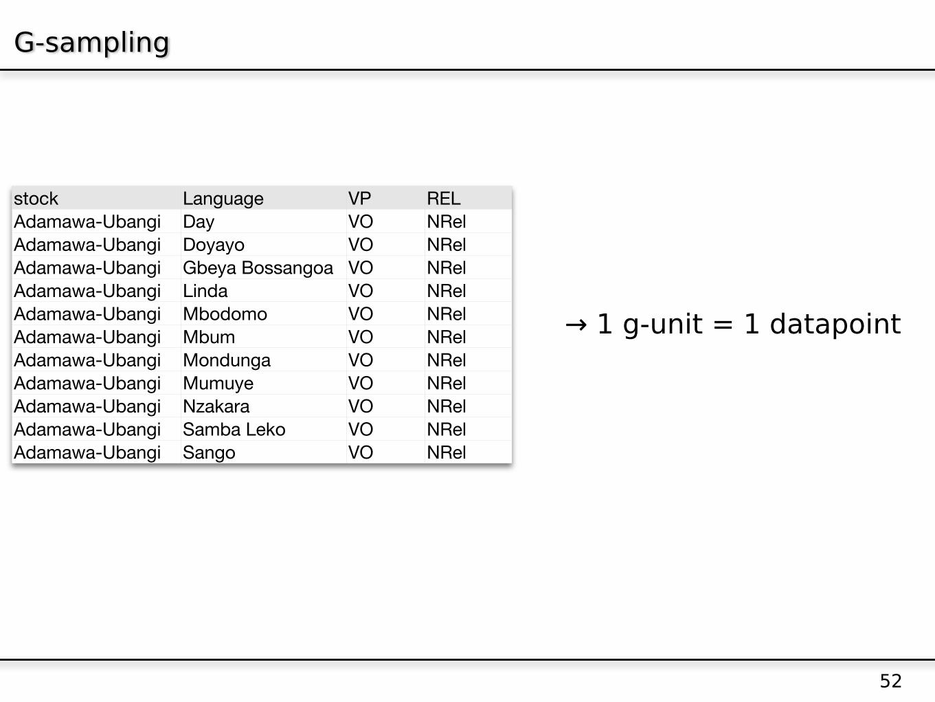
G-sampling

52

stock Language VP RELAdamawa-Ubangi Day VO NRelAdamawa-Ubangi Doyayo VO NRelAdamawa-Ubangi Gbeya Bossangoa VO NRelAdamawa-Ubangi Linda VO NRelAdamawa-Ubangi Mbodomo VO NRelAdamawa-Ubangi Mbum VO NRelAdamawa-Ubangi Mondunga VO NRelAdamawa-Ubangi Mumuye VO NRelAdamawa-Ubangi Nzakara VO NRelAdamawa-Ubangi Samba Leko VO NRelAdamawa-Ubangi Sango VO NRel

→ 1 g-unit = 1 datapoint

Bickel, in press in Sprachtypologie und Universalienforschung 2008

G-sampling

53

stock Language VP RELSino-Tibetan Bai VO RelNSino-Tibetan Cantonese VO RelNSino-Tibetan Hakka VO RelNSino-Tibetan Mandarin VO RelNSino-Tibetan Karen (Bwe) VO NRelSino-Tibetan Karen (Pwo) VO NRelSino-Tibetan Karen (Sgaw) VO NRelSino-Tibetan Kayah Li (Eastern) VO NRelSino-Tibetan Achang OV RelNSino-Tibetan Akha OV RelNSino-Tibetan Apatani OV RelNSino-Tibetan Athpare OV RelNSino-Tibetan Balti OV RelNSino-Tibetan Burmese OV RelNSino-Tibetan Byangsi OV RelNSino-Tibetan Camling OV RelNSino-Tibetan Chantyal OV RelNSino-Tibetan Chepang OV RelNSino-Tibetan Chin (Siyin) OV RelNSino-Tibetan Mishmi (Digaro) OV RelNSino-Tibetan Dimasa OV RelNSino-Tibetan Gallong OV RelNSino-Tibetan Gurung OV RelNSino-Tibetan Hani OV RelNSino-Tibetan Hayu OV RelNSino-Tibetan Jinghpo OV RelNSino-Tibetan Khaling OV RelNSino-Tibetan Kham OV RelNSino-Tibetan Lahu OV RelNSino-Tibetan Limbu OV RelNSino-Tibetan Maru OV RelN

Sino-Tibetan Meithei (Manipuri) OV RelNSino-Tibetan Mising OV RelNSino-Tibetan Mao Naga OV RelNSino-Tibetan Nar-Phu OV RelNSino-Tibetan Newar (Dolakha) OV RelNSino-Tibetan Newar (Kathmandu) OV RelNSino-Tibetan Nocte OV RelNSino-Tibetan Purki OV RelNSino-Tibetan Rawang OV RelNSino-Tibetan Sikkimese OV RelNSino-Tibetan Tamang OV RelNSino-Tibetan Thulung OV RelNSino-Tibetan Tibetan (Modern Literary) OV RelNSino-Tibetan Angami Naga OV NRelSino-Tibetan Garo OV NRelSino-Tibetan Pattani OV NRel

Dryer/WALS: 4 g-units

Bickel, in press:OV RelN 36 1 (trend in ST)OV NRel 3 3 (deviant within OV)VO RelN 4 1 (trend in ST)VO NRel 4 4 (deviant within VO)

Issues of time depth

•If such a g-sample shows an effect, there may be a universal at work at a time depth that is too large to leave a signal in reconstructible taxonomies.

•But, at this time depth, we can’t determine whether the distribution is independent of very ancient skewings, precisely because we know that the variables are super-stable (Maslova 2000).

54

Alternative methods that have been proposed

•Dryer 1989, 2000: use g-samples throughout

•Problem: no guarantee that the g-sample picks up a stationary distribution rather than some unreconstructible earlier areality or other incidents (Maslova 2000).

•Maslova 2000, 2007: compute universally constant rates of change (‘transition probabilities’, akin to biological clocks)

•Problems:

•there are no constant rates of change in language!

•unclear how the method works for multifactorial designs

•computation is based on language pairs, but families are often larger (a sampling problem)

55

Alternative methods that have been proposed

•However, for all its methodological problems, Dryer-style genus sampling has the distinct advantage that it can include isolates; both Maslova’s and my method can be only be applied to families with more than one member.

•And, g-sampling has a very useful, practical cousin: pre-defined standard samples, e.g. the WALS 200-languages sample.

56

Discussion

•Reconciliation: for many hypotheses considered sofar, the methods lead to converging results

•Results of statistical analysis of the g-sampled data: no evidence for an interaction term, but also no evidence for an area effect, i.e. the best-fitting model is:

57

Skewed Family Method: G-sampling Method:

Pro

port

ion o

f fa

milie

s

skew

ed t

ow

ard

s c

ase

Other Eurasia

Pro

port

ion o

f genealo

gic

al unit

s

wit

h independent

pre

sence o

f case

Other Eurasia

Overall conclusions

•Linguistics can move towards standard methods shared with other sciences by

•measuring instead of reducing variation

•interpreting empirical universals in regression models

•which allow statistical estimation of ‘competing factors’ from structure, language contact and other domains

•and can be tested by Monte-Carlo permutation

58

Overall conclusions

•However, the most challenging part in this is to control for blind inheritance effects. This can be done through

•the Skewed Family Method (capturing the dynamics of universals but leaving out isolates) or

•the G-Sampling Method (presupposing stationary distributions but including isolates)

59

Overall conclusions

•What is a ‘universal’ then?

•Empirical universal = sign. structural factor in a model

•Absolute universal = the terms of our metalanguage descriptively needed in every language = that which necessarily follows from the Descriptive A Priori

•What do we urgently need?

•More fine-grained and more precise systems of analytical variables (inventories of types) that accomodate all sources of variation.

•More research on families and subgrouping

•Detailed research on each factor to be entered into a model

60

Documents

Understanding Typological Distributions II · 2. Measuring variation in p-domains ... (17) Bickel, Hildebrandt, & Schiering, ... Dutch French (colloquial) Garo Greek (modern) Hayu