Embed Size (px)
Citation preview

Understanding the Limit Order Book:
Conditioning on Trade Informativeness
Helena Beltrana Joachim Grammigb Albert J. Menkveldc
February 2005
Abstract
Electronic limit order books are ubiquitous in markets today. However, theoretical models
for limit order markets fail to explain the real world data well. Sandas (2001) tests the
classic Glosten (1994) model for order book equilibrium and rejects it. We reconfirm this
result for one of the largest European stock markets. We then relax one of the model’s
assumptions and allow the informational content of trades to change over time. Adapting
Hasbrouck’s (1991a,b) methodology to estimate time varying trade informativeness we
find that it is a slowly mean reverting process. By conditioning on trade informativeness,
we find support for the Glosten model’s implication that books are more shallow during
times of informative market orders. However, a high level of liquidity supply is committed
up to an economically significant trade size volume, even when trade informativeness is
high. This can be seen as a vindication of the open order book design which dispenses
with dedicated market makers. We also find evidence for a market order trader population
which is quite heterogenous with respect to price sensitivity.
aUniversite Catholique de Louvain - COREbEberhard Karls Universitat TubingencVrije Universiteit Amsterdam
JEL classification: G10
Keywords: Informational content of trades, limit order book
Contact details authors. Helena Beltran, [email protected], FNRS Research Fellow at the Center
for operations research and econometrics (CORE), Voie du Roman Pays 34, 1348 Louvain-la-Neuve, Bel-
gium, phone: +32 10 478160, fax: +32 10 474301. Joachim Grammig, [email protected],
Eberhard Karls Universitat Tubingen, Faculty of Economics, Department of Econometrics, Mohlstr.
36, 72074 Tubingen, Germany, +49 7071 29 78159, fax: +49 7071 29 5546. Albert J. Menkveld,
[email protected], Vrije Universiteit Amsterdam, FEWEB, De Boelelaan 1105, 1081 HV Amsterdam,
Netherlands, phone: +31 20 4446130, fax: +31 20 4446020. The first author gratefully acknowledges financial
support from the Belgian “Fonds National de la Recherche Scientifique” (FNRS). We are grateful to Deutsche
Boerse AG for providing access to the limit order data. We thank Stefan Frey for his invaluable collaboration
in the reconstruction of the limit order books and in the estimation of the Sandas model. Uwe Schweickert of
Deutsche Boerse acted as liaison with the designers and operators of the Xetra system and offered unpayable
expertise and support without which this paper could not have been written. Finally, we thank Kerstin Kehrle
and Natascha Wagner for research support. The usual disclaimer applies.
1
1 Introduction
An increasing number of financial assets trade in limit order markets the world over. In
such markets, traders can submit market and limit orders. A market order trades at the
best available price posted by previously submitted limit orders that make up the limit order
book. A limit order is a conditional buy or sell at a pre-specified price and is stored in the
book until canceled or hit by an incoming market order.1
In this paper, we aim to understand order book depth by estimating and testing the
Glosten (1994) model directly, as in Sandas (2001), and indirectly through a dynamic setting
that allows for a time-varying level of private information in order flow. In the indirect
test, we estimate the level of private information of the trade, hereafter referred to as trade
informativeness, using the vector autoregressive approach advocated in Hasbrouck (1991a,b).
As theory predicts that the level of private information is a key determinant of the limit order
book equilibrium, we study the state of the book and the trading activity for a cross section
of stocks and condition on the level of trade informativeness.
Theoretical and empirical papers dealing with the behavior of agents and the evolution of
prices in limit order markets abound in the literature. The economic modeling centers around
an allegedly simple trade-off situation. A limit order trades at a better price than a market
order. However, there are two types of costs to submitting a limit order. First, the order
may fail to execute. Second, the order may execute against a market order that is based on
private information. In this case, limit orders trade at the wrong side of the market. This is
referred to as picking-off risk. Various models have been proposed that formalize this trade-
off between prices, execution probability, and picking-off risk. They essentially take either of
two fundamentally different approaches. The first treats the arrival of traders at the market
exogenously and models their decision to submit a limit or market order and, potentially,
conditions on the state of the book (see, e.g., Cohen, Maier, Schwartz, and Whitcomb (1981),
Foucault (1999), Harris (1998), Parlour (1998), Hollifield, Miller, and Sandas (2004), and
Goettler, Parlour, and Rajan (2004)). These models have a rich set of predictions for the
state of the order book at each point in time. The second approach, essentially, endogenizes
trader arrivals, as it retrieves the state of the book from a zero-profit condition on the marginal
limit order. In other words, at each point in time profit opportunities in the book can only
be short-lived as they attract traders who exploit them immediately. Market orders arrive
exogenously in time, consume liquidity, and potentially leave profit opportunities in the book
that are, again, immediately exploited (see, e.g., Glosten (1994), Seppi (1997), and Parlour
1If a limit order is submitted at a price such that it executes immediately (a marketable limit order), we
consider it a market order.
2

and Seppi (2003)).
The distinction in the theoretical literature carries over to the empirical literature. Many
recent studies focus on whether an arriving trader chooses a market or limit order and how
market conditions affect this choice (see, e.g., Biais, Hillion, and Spatt (1995), Griffiths,
Smith, Turnbull, and White (2000), and Ranaldo (2004)). Most of them condition on the
best bid and ask quotes and depth offered at these quotes. Relatively few studies, however,
focus on explaining the state of the order book beyond these quotes. This is surprising as the
best quotes only partially reflect overall liquidity. A nice illustration is the sequential tick size
reduction in the U.S. that led to a 20% reduction in quoted spreads, but, at the same time,
reduced aggregate depth in the order book (see, e.g., NYSE (2000), Goldstein and Kavajecz
(2000)). Sandas (2001) tests the celebrated Glosten (1994) model and rejects it for a sample
of Swedish stocks. Coppejans, Domowitz, and Madhavan (2003) study order book resiliency
to shocks in volatility and returns for the Swedish stock index future.
We contribute to the literature in two ways. First, we consider the state of limit order
books in a dynamic setting with time-varying order informativeness. This, essentially, allows
us to test the importance of “picking-off” risk, a key ingredient to limit order book models.
If the market can expect very informative order flow, the book should be shallow. We adapt
the standard Hasbrouck (1991a) methodology to estimate trade informativeness. Second, we
use a new dataset with full order book data for arguably one of the largest fully electronic
markets, the German stock exchange. We perform our tests based on market event data for
the thirty stocks that constitute the DAX30 index, the leading German stock market index.
The data are rich as they contain real time limit order book information. The sample runs
from January 2, 2004 through March 31, 2004. We consider this an ideal laboratory for a
test of the Glosten model, as the market runs off of a fully electronic consolidated limit order
book and therefore closely resembles the idealized set-up studied by Glosten. The current
experiment compares favorably to the NYSE order book, as the latter allows for ex-post
quote improvement by the specialist or floor brokers. This seriously undermines the Glosten
framework, as the probability of limit order execution critically depends on the full market
order being executed against the order book.2
The main results can be summarized as follows: Although, consistent with Sandas’ (2001)
findings, we reject, on statistical grounds, Sandas version of the Glosten (1994) model, we
find evidence that “picking-off” risk is important for order book depth in our dynamic set
up. When the market can expect informative market orders, given all history, depth in
the book is considerably lower. These effects are also economically significant, since order
book liquidity, as measured by immediate price impact, is 1.5 times lower at times of high
informativeness. We find that trade informativeness can be described as a stationary and
slowly mean-reverting process. In addition to the state of the book, we study market order
2We refer to Parlour and Seppi (2003) for an excellent analysis of the two market structures: a fully
electronic market and a hybrid market.
3
sizes and trade durations conditional on order informativeness. We find evidence of larger
market order sizes and slightly shorter durations at times when upcoming market orders
are expected to be less informative. We also find evidence for a heterogenous market order
trader population. Part of the market order traders is very price sensitive in that they adapt
market order volumes to the liquidity state of the book. However, another part of the market
order traders do not reduce trade sizes in response to a reduction of liquidity supply. An
important result regarding the assessment of market quality is that a high level of liquidity
supply is committed up to an economically significant trade size volume, even during periods
when trades are allegedly informative. The fact that this conclusion is also valid for smaller
capitalized, less frequently traded stocks is a vindication of the limit order book trading design
and its viability without dedicated market makers.
The remainder of the paper is structured as follows. Section 2 introduces the Xetra open
book and the data used in this paper. In section 3.1 we present a direct test of the Glosten
(1994) model based on Sandas’ (2001) framework. The following section is devoted to explain
the methodology that we employ to estimate the time-varying level of trade informativeness
and its relation to the order book. Section 3.3 presents and discusses the results and section
4 concludes.
2 Market structure and the data
2.1 The Xetra open order book
Xetra is an open order book system developed by the German Stock Exchange.3 It has
operated since 1997 as the main trading platform for German blue chip stocks at the Frankfurt
Stock Exchange. Between an opening and a closing call auction - and interrupted by another
mid-day call auction - trading is based on a continuous double auction mechanism with
automatic matching of orders based on the usual rules of price and time priority. During pre-
and post-trading hours it is possible to enter, revise and cancel orders, but order executions
are not conducted (even if possible). Trading hours extend from 9 a.m. CET to 5.30 p.m.
CET For the DAX30 stocks there are no designated market makers. Traders have access to
the full order book, except hidden shares coming from so-called iceberg orders. An iceberg or
‘hidden’ order is similar to a limit order in that it has pre-specified limit price and volume.
The difference is that a portion of the volume is kept hidden from the other traders.The visible
portion of the iceberg order, called the ‘peak’, enjoys full price and time priorities (as any
limit order). The hidden portion only gets price priority. All disclosed volumes are executed
first, even if those volumes entered the book after the iceberg order submission. When a
market order hits the hidden portion, a new portion of the iceberg order (equal to the peak
size) is revealed to the market participants and is granted time priority over subsequent order
3See Deutsche Borse AG (1999) for a detailed description of the Xetra system.
4
submissions. Consequently, a trader submitting a market order may receive an unexpected
price improvement if her market order is executed against a hidden order. Iceberg orders are
convenient for some market participants as they provide a tool to hide investment decisions.
Whether those decisions are liquidity-motivated or informed remains an open question. In
the realm of limit order book markets, the Xetra system is thus very close to the Euronext
trading system (at the time of this writing, the Euronext trading system encompasses the
Amsterdam, Brussels, Lisbon and Paris stock exchanges), see e.g. Biais, Hillion, and Spatt
(1995). Xetra is also very close to the trading system used at the Hong Kong stock exchange,
which has been recently studied by Ahn and Cheung (1999), Brockman and Chung (1999)
or Ahn, Bae, and Chan (2001). A Xetra market design feature which makes the data for the
purpose of our study preferable is that market orders exceeding the volume at the best quote
are allowed to ‘walk up the book’. In other words, market orders are guaranteed immediate
full execution, at the cost of incurring a higher price impact on the trades. The liquidity
measure used in the present chapter and discussed in the next subsection implicitly assumes
that a ‘walk up the book’ is possible.
2.2 Data
The German Stock Exchange granted access to a database containing complete information
about Xetra order book events (entries, cancelations, revisions, expirations, partial-fills and
full-fills of market, limit, and iceberg orders) that occurred during the first quarter of 2004
(January 2, 2004 - March 31, 2004). The data encompasses the 30 stocks belonging to the
DAX30 index. Based on the event histories we perform a real time reconstruction of the order
book sequences. Starting from an initial state of the order book, we track each change in the
order book implied by entry, partial or full fill, cancelation and expiration of market, limit,
and iceberg orders. This is done by implementing the rules of the Xetra trading protocol
in a GAUSS program. Although running an exhaustive battery of consistency checks no
errors occur during the reconstruction process. From the resulting real-time sequences of
order books, snapshots of the book during the continuous trading hours were taken each time
a trade takes place (just before its matching with the book). For each snapshot, the order
book entries were sorted on the bid (ask) side in price descending (price ascending) order. As
iceberg orders are not fully disclosed to market’s participants, we reconstruct, at each point
in time, two limit order books. First, we have the visible order book, which contains all limit
orders as well as the visible portion of the iceberg orders. Second, we study the complete
order book that features all orders, including the hidden portions.
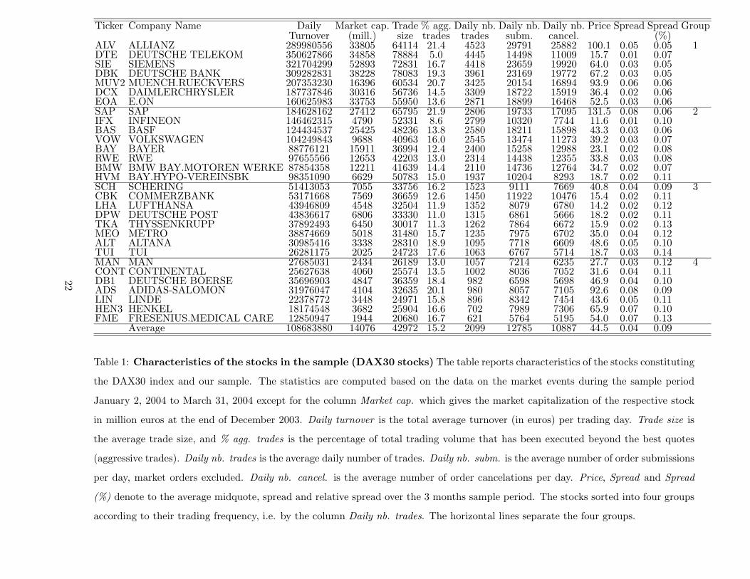
Table 1 presents some characteristics of the DAX30 stocks. Liquidity supply for these
stocks is indeed quite active, as on average 13,000 (11,000) non-marketable limit orders per
stock are submitted (canceled) each day. Implicit transaction costs are relatively small with
relative spreads ranging from 0.04 to 0.14%. On average, 2,100 trades per stock are executed
5

each day and on average 15.2% of these walk up the book (i.e. they are matched by standing
limit orders beyond the best bid and ask prices). We refer to those events as ‘aggressive
trades’.
We adopt a classification of the 30 DAX stocks in four groups based on trading activity.
Indeed, the analysis centers on the impact of trades on liquidity; it is then natural to group
stocks by the number of trades executed each day (on average). The first group is then
composed by the 7 stocks more frequently traded stocks whereas the 7 less frequently traded
stocks are in group 4. The second and third group contain 8 stocks each.4
3 Methodology and Results
3.1 A direct test of the Glosten model
Sandas (2001) presents a variant of Glosten’s (1994) limit order book model with discrete
price ticks and price priority rules. The model delivers an equation that predicts that or-
der book depth and adverse selection effects are inversely related. The associated empirical
methodology is closely based on economic theory and permits the quantification of the rela-
tion of adverse selection effects and order book depth we are after. Since the Xetra trading
protocol is quite close to the idealized framework assumed in Sandas (2001), adopting the
approach for the present paper seems a natural starting point.
In the following we will briefly describe the key ingredients of the Glosten/Sandas frame-
work. The fundamental asset value vt is described by a random walk with innovations depend-
ing on an adverse selection parameter α, which gives the informativeness of a signed market
order of size Xt. The price impact of a trade is linear, immediate and not state-dependent,
viz
vt = cv + vt−1 + αXt + ηv,t. (1)
Negative values of Xt denote sell orders, positive values buy orders. Furthermore, it is assumed
that E(Xt) = 0. ηv,t is an innovation orthogonal to vt−1 and Xt. cv gives the expected
change in the fundamental value. Market buy and sell orders are assumed to arrive with
equal probability with a two-sided exponential density describing the distribution of order
sizes Xt:
f(Xt) = {1
2λe
−Xtλ if Xt > 0 (market buy)
1
2λe
Xtλ if Xt < 0 (market sell).
(2)
Risk neutral limit order traders face a fixed order submission cost γ and have knowledge
about the distribution of market order size and how informative market orders are, that is,
they know α. They do not know the true value of the security, but estimate it conditional
on market order size. They choose limit order prices and quantities such that the expected
4The classification by trading activity is very similar to a classification by market capitalization.
6
profit is maximized. If the last unit at any discrete price tick exactly breaks even, i.e. has
expected profit equal to zero, the order book is in equilibrium.
Denote the ordered discrete price ticks on the ask (bid) side by p+k (p−k) with k = 1, 2, . . .
and the associated volumes at these prices by q+k (q−k). Given these assumptions and setting
q0,t ≡ 0, the equilibrium order book at time t can recursively be constructed as follows:
q+k,t =p+k,t − vt − γ
α−
+k−1∑
i=+1
qi,t − λ k = 1, 2, . . . (ask side)
q−k,t =vt − p−k,t − γ
α−
−k+1∑
i=−1
qi,t − λ k = 1, 2, . . . (bid side). (3)
Equation (3) gives the theoretical model’s answer to the question that motivates the present
paper: order book depth and adverse selection component are inversely related. If the model
provides a good description of the real world trading process, and if we can provide consistent
estimates of the model parameters, we can use equation (3) to predict the evolution of the
order book for a given stock and quantify adverse selection effects on order book depth.
Sandas (2001) proposes to employ GMM for parameter estimation and specification testing.
Assuming mean zero random deviations from the order book equilibrium at each price tick,
the following unconditional moment restrictions, referred to as break-even conditions, can be
used for GMM estimation:
E
(
p+k,t − p−k,t − 2γ − α
(
+k∑
i=+1
qi,t +−k∑
i=−1
qi,t + 2λ
))
= 0 k = 1, 2, . . . (4)
A second set of moment conditions, referred to as updating restrictions, relate the expected
changes in the order book to the market order flow:
E
(
∆p+k,t − α
(
+k∑
i=+1
qi,t+1 −+k∑
i=+1
qi,t
)
− cv − αXt
)
= 0 k = 1, 2, . . .
E
(
∆p−k,t + α
(
−k∑
i=−1
qi,t+1 −−k∑
i=−1
qi,t
)
− cv − αXt
)
= 0 k = 1, 2, . . . (5)
where ∆pj,t = pj,t − pj,t−1. An obvious moment condition to identify the expected market
order size is given by
E(|Xt| − λ) = 0. (6)
Using the DAX30 order book data we estimate the model parameters exploiting the break-
even conditions (4) and the updating conditions (5) along with (6). To construct the moment
conditions we use the respective first four best quotes, i.e. k = 1, . . . , 4 on the bid and the
ask side of the order book. This yields 13 moment conditions, four break-even conditions,
eight update conditions plus the moment condition (6). For convenience, order sizes Xt are
7

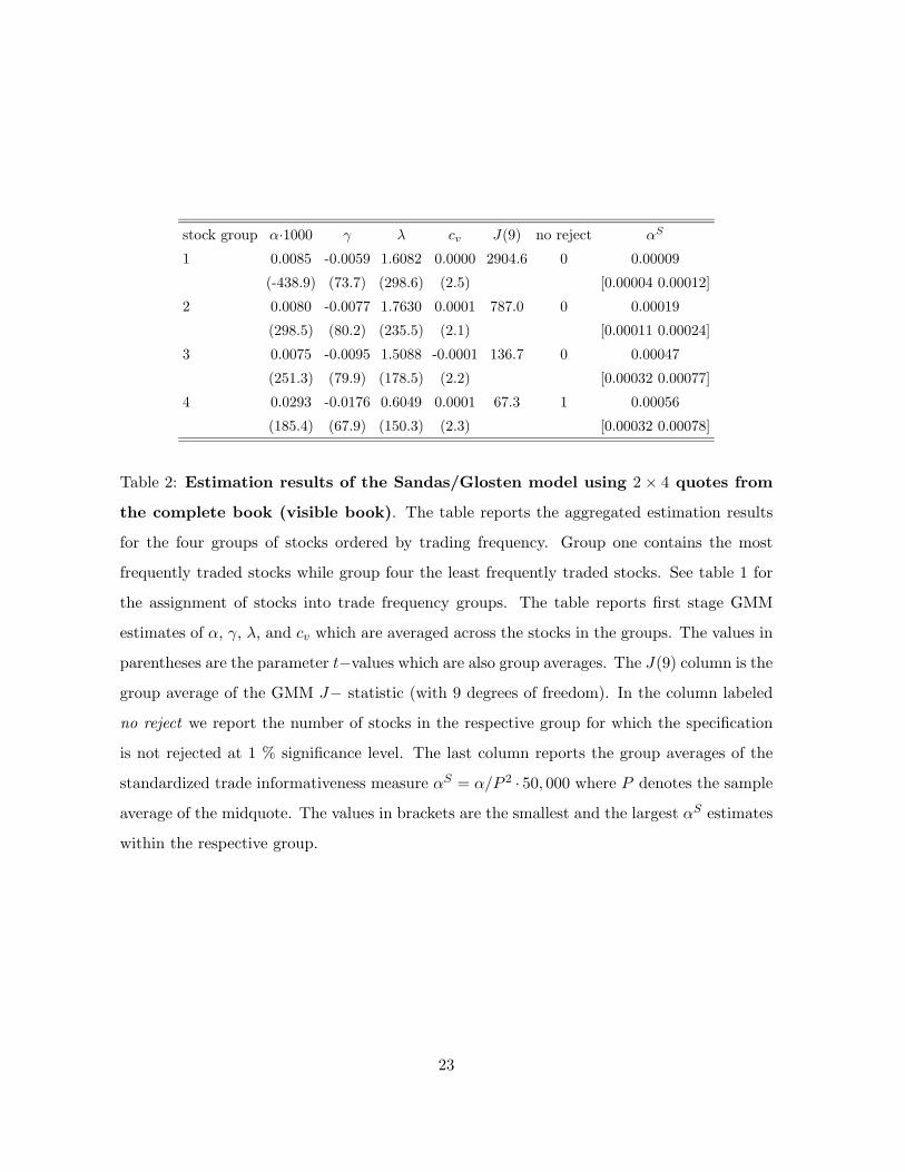
expressed in 1000 shares. Table 2 contains the first stage GMM results for the 4 groups.
We report parameter estimates, t−statistics and the value of the GMM J−statistic with
associated p−values. Under the null hypothesis that the moment conditions are correctly
specified, the J−statistic is asymptotically χ2 with degrees of freedom equal to the number of
moment conditions minus the number of estimated parameters. We also report a standardized
adverse selection component computed as αS = α·50,000P 2 , where P is the sample average of the
midquote of the respective stock. The parameter α measures the absolute impact on prices
of a buy of one share while the standardized measure αS measures the impact on prices in
basis points of a 50,000-euro buy. This standardization ensures comparability of the adverse
selection component across stocks.5
To conserve space and highlight the central findings table 2 presents first stage GMM
estimation results summarized for four stock groups. The thirty stocks are sorted according
to their trading frequency. The first group contains the most frequently traded stocks, the
fourth group the least frequently traded stocks. The information which stock belongs to which
group is presented in table 1. The first stage GMM estimation results are in line with the
central findings reported in Sandas (2001).6 For only one out of thirty stocks the model is
not rejected at 1 % level of significance (in Sandas’ application the model was rejected for all
stocks). Like in Sandas’ (2001) application, the transaction cost estimates (γ) are significantly
negative for all stocks, a result that is difficult to reconcile with the underlying theoretical
model. From an economic point of view, the drift parameter (cv) estimates are small, and not
significantly different (at 1 %) from zero for half of the stocks. This is not surprising given
the high trading frequency. There is a considerable variation in the standardized adverse
selection component αS across stocks. Less frequently traded and small cap stocks tend to
have larger adverse selection components: the Spearman rank correlations of αS and the daily
number of trades and the market capitalization both amount to -0.92. This confirms previous
results which have shown that adverse selection effects are more severe for less frequently
traded, smaller capitalized stocks. In itself, these are interesting results, yet with considerable
amounts of grains of salt given the unsatisfactory empirical performance reported above. This
is a familiar trade-off. Although a formal model like the Sandas/Glosten framework delivers
economically interpretable parameter estimates, some assumptions required to provide closed
form moment conditions for parameter estimation may be too restrictive and responsible for
the discontenting performance when the model is confronted with real world data. Specifically,
it could be argued that the linearity, state-independence and immediacy of the price impact of
trades implied by equation (1) is incompatible with a dynamic order book. Sandas (2001) dealt
with this issue by introducing state variables that describe the time dependence of the model
5One share costs 1/P euros, therefore a trade of 50,000 euros amounts to 50, 000/P shares. α/P measures
the impact on prices in basis points of a one-share buy. We also computed a standardized α based on the
(stock-specific) average trade size; the results presented below were not affected.6Second stage and iterated GMM results are qualitatively identical and lead to the same conclusions.
8
parameters. The advantage of this approach is that one can stay within the GMM estimation
and testing framework. However, the choice of plausible state variables is rather ad hoc and
not guided by theory. In the following we will pursue an alternative approach to investigate
the relation of the informational content of the order flow and order book variation. For this
purpose we reconsider a classic approach developed by Hasbrouck (1991a,b) and adapt it for
our purpose.
3.2 Allowing for time-varying trade informativeness
In the previous section a series of restrictive assumptions have been made to obtain estimable
equations and estimates of trade informativeness derived from order book equilibrium con-
ditions. As argued above, the assumption that the trade informativeness parameter α is
time-invariant seems restrictive. Some restrictions are already planted in Glosten’s basic
theoretical framework. Specifically, variations in the book caused by non-informationally mo-
tivated agents who choose strategically between limit and market orders (as e.g. in Foucault,
Kadan, and Kandel (2003)) are explicitly not accounted for. Although these two streams in
the theoretical literature - the one focussing on adverse selection effects, the other on strategic
trading - are antinomic, it is reasonable to assume that both explain important aspects of the
trading processes in real world limit order markets.
We deal with these shortcomings in an alternative econometric framework. To estimate
trade informativeness, we reconsider the classic approach introduced by Hasbrouck (1991a,b)
and adapt this methodology to allow for time varying trade informativeness. The resulting
estimates are then used to study the relation of trade informativeness and the state of the
order book. Unlike in the direct test of the Glosten model, no prior assumption is imposed
on the trade informativeness-book relation. Furthermore, the possibility of changes in the
book originating from non-informationally induced, serially correlated liquidity shocks is not
ruled out. We will briefly review Hasbrouck’s methodology and show how it is adapted for
the present paper. The basic idea is to estimate trade informativeness by the long-run impact
of a trade on the prices computed from a two variable vector autoregression (VAR). This
methodology offers a straightforward way to disentangle short term microstructure effects
from permanent information. Inventory management and lagged price adjustments do not
prevent prices to ultimately incorporate the informational content of a trade.
Hasbrouck’s VAR contains two variables. The first is the midquote difference, rt = qt −
qt−1, where qt = (p1,t +p−1,t)/2. The second variable Xt denotes, as above, the signed market
order size. The subscript t refers to event time, i.e. every time there is a trade or a midquote
update, t is incremented by one. rt is zero if at time t there is a trade without any change
in the midquote. When the midquote changes at time t without a trade event then Xt = 0.
9

Setting up the VAR as
rt = a1rt−1 + a2rt−2 + . . . + b0Xt + b1Xt−1 + b2Xt−2 + . . . + v1,t
Xt = c1rt−1 + c2rt−2 + . . . + d1Xt−1 + d2Xt−2 + . . . + v2,t, (7)
contemporaneous causality from trades to prices is accounted for. In a pure order book this
effect could be truly contemporaneous as trades frequently walk up the book and consume the
liquidity available at the best quotes and thus induce an immediate change of the midquote.
The Vector Moving Average (VMA) representation of the VAR 7 is given by
rt = v1,t + a∗1v1,t−1 + a∗2v1,t−2 + . . . + b∗0v2,t + b∗1v2,t−1 + b∗2v2,t−2 + . . .
Xt = c∗1v1,t−1 + c∗2v1,t−2 + . . . + v2,t + d∗1v2,t−1 + d∗2v2,t−2 . . . . (8)
The parameter b∗0 gives the immediate impact of an unexpected buy of one share on the
midquote, The permanent impact of an one unit (buy) trade innovation is given by α∗ =∑
∞
i=0b∗i . While short-lived inventory or microstructure effects may move the midquote away
from the efficient price, α∗ serves a natural measure of the permanent effect of trade related
information on the asset price. It is the counterpart of the Glosten/Sandas-α (see equation
1) and directly comparable in levels.
Traders are likely to update their beliefs about the information content of trades con-
tinuously. Ideally, an econometrician would update her estimate of trade informativeness
whenever there is an update in traders’ beliefs. This is of course impossible. As a feasible
approximation we fix the number of trade events N that have to occur before a new VAR esti-
mation is conducted, and a new measure of trade informativeness is computed. This produces
a sequence of trade informativeness measures {α∗
j}(j = 1, ..., J), each estimated from data
on N successive trade events. We also retrieve a sequence of estimated immediate impacts
{b∗0,j}(j = 1, ..., J).7 α∗
j can be interpreted as the average of the true, but non observable
time varying trade informativeness over the jth estimation period. As long as the updates
on trade informativeness are smooth, this approximation seems not overly restrictive.
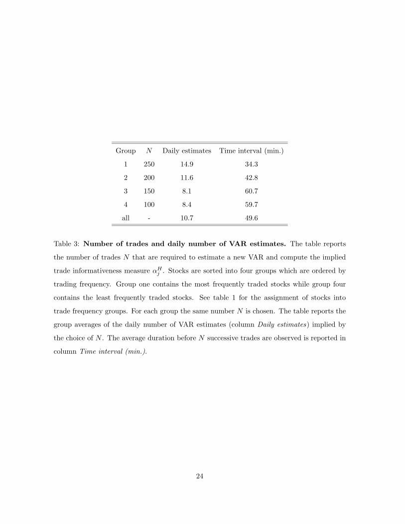
Table 3 reports some details about the specifications. For the group of less frequently
traded stocks we choose N = 100 trades. This implies that on average a new estimate of α∗
j is
computed every 60 minutes. For the group of most frequently traded stocks, we use N = 250.
In this case a new trade informativeness measure is computed on average every 30 minutes.
Sensitivity tests which involved changing the number of trades events N were conducted, but
the results do not change substantially. The number of lags in the VARs is 10 for all stocks
which ensures serially uncorrelated residuals. We follow Hasbrouck and truncate the infinite
7An alternative would be to fix the number of quotes or events. However, quote updates are quite frequent
in the order book market that we study. One can observe hundreds of quote updates without any trade
event. By setting a fixed number of trades instead of a fixed number of events, we avoid estimating trade
informativeness with only few number of trade events.
10
sum over the VMA parameters at 40 steps, i.e. α∗ =∑
40
i=0b∗i (omitting the j subscript).We
do not regress today’s trades and quotes on yesterday’s. Instead, we re-initialize the VARs
at the start of each trading day. To ensure cross sectional comparability, we standardize α∗
j
in the same fashion as the Glosten/Sandas-α viz,
αHj =
α∗
j · 50, 000
P 2. (9)
Thus, αHj is the long-term impact in basis points of an (unexpected) 50,000-euro buy. The
sample average αH = J−1∑
αHj can be directly compared to the standardized trade informa-
tiveness measure αS which has been used in the Glosten/Sandas framework. The immediate
impact b∗0,j can be standardized in the same fashion. The resulting sequence will be denoted
by {bHj }(j = 1, ..., J). Computing bH = J−1
∑
bHj allows to compare the levels of the av-
erage short run effect of trades on prices with the average permanent impact αH and the
Sandas/Glosten measure of trade informativeness, αS .
3.3 Cross sectional and time series properties of trade informativeness
Table 4 summarizes the time series properties of the estimates of the standardized trade
informativeness measures αHj and the standardized immediate price impacts bH
j as well as the
corresponding cross sectional variation of the sample averages αH and bH . In line with the
results discussed in section 3.1 we find that trade informativeness estimates tend to be smaller
for frequently traded stocks and higher for less frequently traded stocks. The group specific
averages of αH are strikingly similar to the GMM estimates of the trade informativeness
measures αS in the Glosten/Sandas framework (compare the first column of table 4 and the
last column of table 2). On the other hand, the group averages of the αH estimates (and of
αS) are almost two times larger than the average of the estimated immediate impacts bH .
Hence, the GMM estimates of αS seem to capture the long-term impact of a trade. At first
sight this may seem surprising, since equation (1) postulates an immediate impact of signed
trades. However, the immediate effect is exerted on the unobservable fundamental asset
value. The VAR in equations (7), however, is estimated on observable midquote changes.
The midquote arguably serves as a proxy for the fundamental value, but, as discussed above,
it may deviate from the fundamental value due to microstructure effects. In fact, it turns out
that in Sandas’ GMM setting framework the (static) break-even order book conditions are the
most important moment restrictions to infer the trade informativeness estimate parameter
α.8 Sandas’ theory based, yet restrictive GMM approach to estimate trade informativeness
is quite different from the agnostic yet less restrictive VAR approach. The result the trade
informativeness estimates delivered by both methodologies are quite similar indicates that
8As in Sandas (2001) the update conditions do not help greatly for the identification of α. The standard
errors of the α estimates are very large if only update conditions are used for GMM estimation. The update
restrictions are more important to identify the drift parameter cv.
11
the formal Glosten/Sandas framework is not as much at odds with the data as the rejection
based on statistical tests suggests.
While this can be interpreted as a vindication of the Sandas/Glosten theoretical framework
the results reported in table 4 and the time series plots in figure 1 also show that the trade
informativeness sequences {αHj } exhibit a considerable variation. Figure 1 plots the estimated
{αHj } sequence for selected stocks, one from each of the four groups sorted by trade-frequency.
From time series perspective one may describe these data a being generated by a mean
reverting process. Table 4 reports the minimum and maximum of the αHj estimates averaged
over the stocks in the respective group. Figure 2 which plots time-of-day averages of αHj for
half hour intervals shows that the trade informativeness estimates exhibit a distinct intra-
day (diurnal) pattern. Trade informativeness is (on average) highest at the beginning of
the trading day, but drops to a lower level during the two hours or so after the opening.
For the more frequently traded stocks trade informativeness increases during the overlap
period with NYSE trading. It seems that the beginning of US trading of the respective
stock initiates another trade informative period. All the stocks belonging to the group of
most frequently traded stocks and half of the stocks belonging to the second group are cross-
listed in an US market (mostly as ADRs at NYSE). The third and the fourth group do
not contain any US cross-listed stock. To some extend, these time-of-day patterns are in line
with findings of studies which used different methodologies to analyze time-of-day variations of
trade informativeness in other markets.9 The variation of estimated αHj over time corroborates
the conjecture that part of the rejection of the Sandas specification originates in the neglected
variation of the adverse selection parameter α.
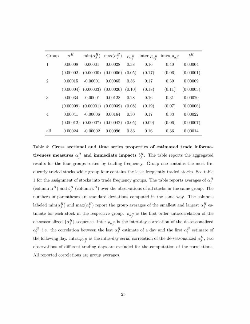
To study the serial dependence of the trade informativeness measures in greater detail,
we de-seasonalize the data by subtracting the stock specific time-of-day (half-hour) average
from αHj . Table 4 reports the serial correlation, inter-day correlation, and intra-day correla-
tion of the diurnally adjusted sequence {αHj }. Figure 3 plots the autocorrelation functions
(ACFs) averaged across the four stock groups. The first order autocorrelation of the season-
ally adjusted trade informativeness measure (ραHj
) ranges from 0.28 to 0.38. This means that
trade-informative periods are clustered. A period where trade informativeness is high (more
precisely higher than the time-of-day average) tends to be followed by another informative
period. Intra-day serial dependence of trade informativeness is stronger than inter-day de-
pendence. This can be seen by comparing the correlation between the last estimate of αHj for
a trading day and the first estimate of the following trading day (inter ραHj
) with the pure
intra-day correlation (intra ραHj
) which excludes successive observations that do not belong to
the same trading day. Table 4 shows that the inter-day correlation is considerably lower than
the intra-day serial correlation. This implies that informative periods do not tend to extend
across trading days. The intra-day serial correlation of the trade informativeness measure
9Ahn, Cai, Hamao, and Ho (2002) decompose the spread in a pure limit order book market (Tokyo Stock
Exchange) and found that the adverse selection component of the spread exhibits a ∪-shape.
12
does not vary greatly between stock groups. It lies between 0.40 (average of first group, most
frequently traded) and 0.31 (average of third group).
3.4 Book liquidity, trading activity, and trade informativeness
Figures 4 to 8 illustrate graphically the relation of book liquidity measures and trading activity
on the one hand and the degree of informativeness of trades on the other. Each figure consists
of four panels which display the results for the four groups of stocks sorted by the trading
frequency (trade frequency quartiles). In each of the graphs, the values on the horizontal axis
are the deciles of the standardized adverse selection component αHi . To compute the deciles,
we pool all observations of the stocks belonging to the same trading frequency group. The
observations are trade events for which we measure trading volume (in euros), the duration
since the last trade, and the prevailing relative inside spread (best bid minus best bid offer
divided by midquote) prior to the trade. To each trade event we assign the αHj of the
estimation window to which the respective trade event belongs to.
In an open limit order book market it is especially interesting to study how liquidity
beyond the best quotes responds to informed order flow. For this purpose, we employ a pre-
trade book liquidity measure similar to those proposed in Irvine, Benston, and Kandel (2000)
and Gomber, Schweickert, and Theissen (2004). The basic idea is to compare the per-share
price of a time t buy or sell order of volume v with the prevailing best ask or bid price,
respectively. The per-share price obtained when selling v shares at time t can be computed
as
bt(v) =
∑
k bk,tvk,t
v, (10)
where v is the volume executed at k different unique bid prices bk,t with corresponding volumes
vk,t standing in the limit order book at time t (this takes into account that the order can ’walk
up the book’). The unit price at(v) of a buy of size v at time t can be computed analogously.
To ensure comparability across stocks, we relate the per-share prices to the best quotes, viz
apt(v) =at(v) − at(1)
at(1)· 100 (11)
and
bpt(v) =bt(1) − bt(v)
bt(1)· 100. (12)
We refer to apt(v) as the ask price impact and to bpt(v) as the bid price impact. These price
impacts serve as natural liquidity measures for an open order book system. They account
for the bi-dimensionality of liquidity supply (price and volume), and are comparable across
stocks.10 To generate the values on the vertical axes of figures 4 to 8, we proceed as follows:
10In fact, the German Stock Exchange employs a closely related concept (denoted XLM, short for Xetra
Liquidity Measure) to monitor and report the quality of liquidity in the Xetra system, both across stocks and
over time.
13
each trade event with corresponding order book snapshot immediately prior to the trade is
assigned to its αH decile. We then compute decile specific means, medians, and 0.75-quantiles
of the trade related variables (volume and duration) and of the variables describing liquidity
displayed in the order book, inside spread as well as the bid and ask price impacts, apt(v) and
bpt(v). We set v equal to an ’average’ volume, v = 50,000 euros, and a ’large’ volume, v =
250,000 euros, respectively. A trade of 50,000 euros roughly corresponds to the average trade
size computed over all thirty stocks, while a trade of 250,000 euros can be considered a large
trade for any of the stocks. Figure 4 shows that the inside spread tends to be higher (smaller)
when trade informativeness is high (low). This is most pronounced for the two groups of
less frequently traded stocks (two lower panels in figure 4). For the group of least frequently
traded stocks the average spread increases from 0.07% to 0.11 % when comparing the 0.1
αH−decile with the .9−decile. Figures 5 and 6 show that liquidity supply beyond the best
quotes, as measured by price impacts, apt(v) and bpt(v), is sensitive towards informational
order flow. Limit order traders demand liquidity premiums for taking the counterpart in
large transactions during times of informational order flow. Both bid and ask side results
support this conclusion. It holds true especially for less frequently traded stocks (see the
lower panels of figure 5 and 6). For example, the average ask price impact for the large
volume, apt(250, 000), increases from 0.13 % (0.1 decile) to 0.33 % (0.9 decile). Therefore,
both in relative and in absolute terms, price impacts increase considerably more than inside
spread. The result that book liquidity beyond the best quotes reacts to informed order flow
concerns also the frequently traded/large capitalized stocks. While the response is comparable
in relative terms, it is smaller in absolute terms. For example apt(250, 000), increases from
0.02 % to 0.05 % in the group of most frequently traded stocks (see upper left panel of figure
5). Measuring liquidity for the ’average’ volume v = 50, 000, the inverse relation of liquidity
supply and trade informativeness is still discernable, but it is weaker. Figures 5 and 6 show
that a relative high level of liquidity supply is committed up to a economically significant trade
size volume, even during periods when trades are allegedly informative. The fact that this
conclusion is also valid for smaller capitalized, less frequently traded stocks can be interpreted
as a vindication of the limit order book trading design and its viability without dedicated
market makers.
Figure 7 shows that trade sizes and trade informativeness are inversely related, with a
considerable decrease of average trading volumes during times of informed order flow. The
finding holds true for all four trade frequency quartiles. For example, in the group of least fre-
quently traded stocks, the average trade size decreases from 35,000 euros in the 0.1 αH−decile
to 20,000 euros in the 0.9 αH−decile. In the group of most frequently traded stocks, the av-
erage trade size in the 0.1 αH−decile amounts to 80,000 euros while in the 0.9 decile the
average trade size is 50,000 euros. Previous studies have already documented that market
order submissions in open order book markets are clearly timed (see Coppejans, Domowitz,
and Madhavan (2002) and Gomber, Schweickert, and Theissen (2004)). Large order sizes are
14

submitted when committed liquidity in the book is high, while at times of reduced liquidity
supply, trade order sizes are smaller. Our results point in the same direction, but they also
highlight an important background variable which affects both book liquidity and order sizes,
namely the degree of informed order flow. We have seen above that adverse selection effects
reduce liquidity supply beyond the best quotes, especially for large volumes.
The considerable reduction of trade sizes during periods of informed order flowsuggests
that market order traders (be they informed or not) are very price sensitive and that they
adapt their market order volumes to the liquidity state of the book. We have seen that
liquidity supply is reduced during periods of informed order flow (especially for large trading
volumes and less frequently traded stocks and to a lesser extend for moderate trading volumes
and frequently traded, large cap stocks). However, the average trade sizes are noticeably
smaller during times of informed order flow. This holds true also for frequently traded stocks,
for which the markups and discounts demanded by limit order traders during periods of
informed order flow are moderate even for large volumes. This results suggests a high price
sensitivity of market order traders. Accordingly, the result that the median trade size does not
change with trade informativeness can be interpreted as evidence for a heterogenous market
order trader population. One group of traders does not reduce trade sizes in response to a
(allegedly informationally induced) reduction of liquidity supply. In line with the reasoning,
these agents may either be impatient informed or price-insensitive traders who are willing to
conduct buy and sell transactions even with some markup or discount on the per share price.
On the other hand, the trader population also seems to contain highly price sensitive traders
who closely monitor the book, time their trades, and who adjust their trade sizes according
to the liquidity state of the book.
While the sensitivity of average trade sizes towards informed order flow is considerable,
trade durations are only marginally affected. Although figure 8 shows a positive relation of
trade informativeness and trade durations, the increase of average trade durations when com-
paring the 0.1 αH−decile with the 0.9 decile seems small in terms of economic significance.
Average trade duration increases by only about 5 seconds even when the informational content
of the order flow is highest. Since the interest in the role of trade durations and their relation
with adverse selection effects has surged (spurred by the papers by Engle and Russell (1998)
and Engle (2000)), this result rewards some further discussion. Dufour and Engle (2000) have
pointed out that the theoretical model of Easley and O’Hara (1992) implies a testable hypoth-
esis about the relation of trading intensity and informed order flow. In a nutshell it works as
follows. During informative periods, traders possessing superior information split their orders
in order to prevent the market maker from identifying their trades as being informationally
motivated. The informed agents submit smaller volumes, albeit more frequently. One would
therefore expect shorter trade durations and smaller volumes during informational periods.
To test this prediction, Dufour and Engle (2000) propose another adaption of the Hasbrouck
(1991a,b) framework which accounts for the alleged relation of trading frequency and trade
15

informativeness. Estimating their model on NYSE data, they find a strong relation between
trade durations and trade informativeness, and interpret this as empirical support for the
validity of the Easley and O’Hara (1992) model. Our results show that this conclusion cannot
be readily transferred to an automated auction system. While the reduction of average trade
sizes during informative periods is compatible with the predictions implied by the Easley and
O’Hara (1992) model, the weak relation of trade informativeness and trade durations is not.
We interpret this result as an outcome of the different market structures. Unlike the NYSE
trading process analyzed by Dufour and Engle (2000), the Xetra automated auction system
employs no central market makers endowed with discretionary pricing power. The NYSE
specialist can grant price improvements over the quoted spreads and is (relatively) free to set
prices for volumes that exceed depth at the best quotes. In the automated auction system,
however, the per share price for a given trading volume is fixed ex ante and also ex post.11 In
other words, liquidity suppliers, unlike the NYSE specialist, do not have the opportunity to
discriminate prices between allegedly informed and uninformed order arrivals. Instead, they
have to take trade informativeness into account prior to the arrival of the market orders. And
in fact, this is what is reflected in our data. We have seen that liquidity committed to the
book does react to trade informativeness. So do the sizes of market orders, as both informed
and uninformed trader population contain price sensitive agents. However, the inverse rela-
tion of trade informativeness and trade durations predicted by the Easley and O’Hara (1992)
seems to be confined to specialist systems.
4 Conclusion and outlook for further research
In this paper we have analyzed how the state of the limit order book and trade informativeness
interact. Following Sandas (2001) we have performed a direct test of the Glosten (1994)
model which provides a closed form expression for the relation of order book depth and trade
informativeness. However, like in Sandas (2001) analysis, the Glosten model is rejected based
on the grounds of formal statistical tests despite the fact that the data generating process
fits the theoretical framework set up by Glosten much better. Given this discontenting result
we develop a more flexible approach based on an adaption of Hasbrouck’s (1991a, 1991b)
methodology and study the relation of trade informativeness and the state of the order book,
market order sizes and trade durations. The main results can be summarized as follows:
• The level of trade informativeness varies greatly and can be described as a slowly mean
reverting process. This result may explain why the theory-based Sandas (2001) model
with time invariant trade-informativeness parameter fails to explain order book data
well.
11For the ask side these prices are given by equation (10).
16
• As predicted in the Glosten/Sandas limit order book model, our methodology confirms
that the book is shallower when trade informativeness is high. Limit order traders
demand liquidity premiums for taking the counterpart in large transactions during times
of informational order flow. This result is most pronounced for less frequently traded
stocks.
• The inside (quoted) spread tends to be larger when trade informativeness is high (low).
However, the effect of an increase of trade informativeness on the inside spread is smaller
than the effect on liquidity beyond the best quotes.
• Average trade sizes are noticeably smaller during times of informed order flow. However,
while the sensitivity of average trade sizes towards informed order flow is considerable,
the effects on trade durations are much smaller. This result indicates the presence of
a heterogenous market order trader population. Part of the market order traders is
quite price sensitive in that they adapt their market order volumes to the liquidity
state of the book. However, another group does not reduce trade sizes in response to
an informationally induced reduction of liquidity supply. Whether these traders are
informed or merely price insensitive and impatient remains an open point.
• Contrary to findings for specialist markets we show that trade durations do not react
in an economically significant way towards trade informativeness. Thus, care should be
taken when applying the conclusions regarding the validity of predictions from theoret-
ical models of specialist market microstructure to automated auction systems.
• In the open order book market that we have studied, a high level of liquidity supply is
committed up to a economically significant trade size volume, even during periods when
trades are allegedly informative. The fact that this conclusion is also valid for smaller
capitalized, less frequently traded stocks is a vindication of the limit order book trading
design and its viability without dedicated market makers.
Avenues for further research stretch in various directions. First, the investigation how
book liquidity reacts to informativeness of trades could be placed in a multivariate empirical
analysis. The objective of this exercise is to assess to which degree order book variation is
attributable to adverse selection effects. We hope that such an analysis will shed light on the
empirical relevance of those two parallel streams in the theoretical literature that explain limit
order book evolution. Second, a drawback of our analysis is that so far we use fixed windows
to estimate the trade informativeness measure. A greater flexibility would be obtained if
the trade informativeness measure would be updated after each trade. Third, we believe
that the methodology presented in this paper could be fruitfully applied to assess issues of
market design in open order book markets. The market structures of the leading European
exchanges are subject to a permanent redesign process. The empirical tools presented in this
17

paper could be used to quantify how the balance of liquidity supply and demand is affected
by these design measures. Furthermore, the favorable conclusion regarding the viability of
the open limit order book market without dedicated market makers are valid for a sample
of stocks in which even the least frequently traded stock was still quite actively traded and
had a rather liquid book. Whether the same conclusion also holds for stocks which do not
belong to a major stock market index is an open question for further research. Finally, it
would be interesting to study liquidity supply for internationally cross listed stocks using the
methodology presented in this paper. The NYSE open book program allows to estimate and
compare the effect of trade informativeness on the liquidity supply of internationally cross
listed stocks.
18
References
Ahn, H., K. Bae, and K. Chan (2001): “Limit orders, depth and volatility: evidence from
the stock exchange of Hong Kong,” Journal of Finance, 56, 767–788.
Ahn, H., J. Cai, Y. Hamao, and R. Ho (2002): “The components of the bid-ask spread
in a limit order market: evidence from the Tokyo stock exchange,” Journal of Empirical
Finance, 9, 399–430.
Ahn, H., and Y. Cheung (1999): “The intraday patterns of the spread and depth in a
market with market makers: the Stock Exchange of Hong Kong,” Pacific-Basin Finance
Journal, 7, 539–556.
Biais, B., P. Hillion, and C. Spatt (1995): “An empirical analysis of the limit order book
and the order flow in the Paris Bourse,” Journal of Finance, 50, 1655–1689.
Brockman, P., and D. Chung (1999): “An analysis of depth behavior in an electronic,
order-driven environment,” Journal of Banking and Finance, 23, 1861–1886.
Cohen, K., S. Maier, R. Schwartz, and D. Whitcomb (1981): “Transaction Costs, Or-
der Placement Strategy and Existence of the Bid-Ask Spread,” Journal of Political Econ-
omy, 89, 287–305.
Coppejans, M., I. Domowitz, and A. Madhavan (2002): “Liquidity in an automated
auction,” Mimeo.
(2003): “Dynamics of Liquidity in an Electronic Limit Order Book Market,” Dis-
cussion paper, Department of Economics, Duke University.
Deutsche Borse AG (1999): “Xetra Market Model Release 3 Stock Trading,” Technical
Report.
Dufour, A., and R. Engle (2000): “Time and the impact of a trade,” The Journal of
Finance, 55, 2467–2499.
Easley, D., and M. O’Hara (1992): “Time and the Process of Security Price Adjustment,”
Journal of Finance, 47, 577–605.
Engle, R., and J. Russell (1998): “Autoregressive conditional duration; a new model for
irregularly spaced transaction data,” Econometrica, 66, 1127–1162.
Engle, R. F. (2000): “The econometrics of ultra-high frequency data,” Econometrica, 68,
1–22.
Foucault, T. (1999): “Order flow composition and trading costs in a dynamic limit order
marker,” Journal of Financial Markets, 2, 99–134.
19
Foucault, T., O. Kadan, and E. Kandel (2003): “Limit order book as a market for
liquidity,” Forthcoming, Review of Financial Studies.
Glosten, L. (1994): “Is the electronic open limit order book inevitable?,” Journal of Fi-
nance, 49, 1127–1161.
Goettler, R., C. Parlour, and U. Rajan (2004): “Equilibrium in a Dynamic Limit
Order Market,” Forthcoming, Journal of Finance.
Goldstein, M., and K. Kavajecz (2000): “Eights, Sixteenths, and Market Depth: Changes
in Tick Size and Liquidity Provision on the NYSE,” Journal of Financial Economics, 1(56),
125–149.
Gomber, P., U. Schweickert, and E. Theissen (2004): “Zooming in on Liquidity,” EFA
2004 Working Paper, University of Bonn.
Griffiths, M., B. Smith, D. Turnbull, and R. White (2000): “The Costs and Deter-
minants of Order Aggressiveness,” Journal of Financial Economics, 56, 65–88.
Harris, L. (1998): “Optimal Order Submission Strategies in Some Stylized Trading Prob-
lems,” Financial Markets, Institutions, and Instruments, 7(2).
Hasbrouck, J. (1991a): “Measuring the information content of stock trades,” Journal of
Finance, 46(1), 179–207.
(1991b): “The Summary Informativeness of Stock Trades: An Econometric Analy-
sis,” Review of Financial Studies, 4(3), 571–595.
Hollifield, B., R. Miller, and P. Sandas (2004): “Empirical Analysis of Limit Order
Markets,” Discussion paper, Forthcoming, Review of Economic Studies.
Irvine, P., G. Benston, and E. Kandel (2000): “Liquidity beyond the inside spread: mea-
suring and using information in the limit order book,” Mimeo, Goizueta Business School,
Emory University, Atlanta.
NYSE (2000): “Presentation at SEC Roundtable discussion on Decimalization, December
11, 2000,” Discussion paper.
Parlour, C., and D. Seppi (2003): “Liquidity-Based Competition for Order Flow,” Review
of Financial Studies, 16(2), 301–343.
Parlour, C. A. (1998): “Price Dynamics in Limit Order Markets,” Review of Financial
Studies, 11, 789–816.
Ranaldo, A. (2004): “Order aggressiveness in limit order book markets,” Journal of Finan-
cial Markets, 7, 53–74.
20

Sandas, P. (2001): “Adverse Selection and Competitive Market making: Empirical Evidence
from a Limit Order Market,” Review of Financial Studies, 14(3), 705–734.
Seppi, D. J. (1997): “Liquidity provision with limit orders and a strategic specialist,” Review
of Financial Studies, 10, 103–150.
21
Ticker Company Name Daily Market cap. Trade % agg. Daily nb. Daily nb. Daily nb. Price Spread Spread GroupTurnover (mill.) size trades trades subm. cancel. (%)
ALV ALLIANZ 289980556 33805 64114 21.4 4523 29791 25882 100.1 0.05 0.05 1DTE DEUTSCHE TELEKOM 350627866 34858 78884 5.0 4445 14498 11009 15.7 0.01 0.07SIE SIEMENS 321704299 52893 72831 16.7 4418 23659 19920 64.0 0.03 0.05DBK DEUTSCHE BANK 309282831 38228 78083 19.3 3961 23169 19772 67.2 0.03 0.05MUV2 MUENCH.RUECKVERS 207353230 16396 60534 20.7 3425 20154 16894 93.9 0.06 0.06DCX DAIMLERCHRYSLER 187737846 30316 56736 14.5 3309 18722 15919 36.4 0.02 0.06EOA E.ON 160625983 33753 55950 13.6 2871 18899 16468 52.5 0.03 0.06SAP SAP 184628162 27412 65795 21.9 2806 19733 17095 131.5 0.08 0.06 2IFX INFINEON 146462315 4790 52331 8.6 2799 10320 7744 11.6 0.01 0.10BAS BASF 124434537 25425 48236 13.8 2580 18211 15898 43.3 0.03 0.06VOW VOLKSWAGEN 104249843 9688 40963 16.0 2545 13474 11273 39.2 0.03 0.07BAY BAYER 88776121 15911 36994 12.4 2400 15258 12988 23.1 0.02 0.08RWE RWE 97655566 12653 42203 13.0 2314 14438 12355 33.8 0.03 0.08BMW BMW BAY.MOTOREN WERKE 87854358 12211 41639 14.4 2110 14736 12764 34.7 0.02 0.07HVM BAY.HYPO-VEREINSBK 98351090 6629 50783 15.0 1937 10204 8293 18.7 0.02 0.11SCH SCHERING 51413053 7055 33756 16.2 1523 9111 7669 40.8 0.04 0.09 3CBK COMMERZBANK 53171668 7569 36659 12.6 1450 11922 10476 15.4 0.02 0.11LHA LUFTHANSA 43946809 4548 32504 11.9 1352 8079 6780 14.2 0.02 0.12DPW DEUTSCHE POST 43836617 6806 33330 11.0 1315 6861 5666 18.2 0.02 0.11TKA THYSSENKRUPP 37892493 6450 30017 11.3 1262 7864 6672 15.9 0.02 0.13MEO METRO 38874669 5018 31480 15.7 1235 7975 6702 35.0 0.04 0.12ALT ALTANA 30985416 3338 28310 18.9 1095 7718 6609 48.6 0.05 0.10TUI TUI 26281175 2025 24723 17.6 1063 6767 5714 18.7 0.03 0.14MAN MAN 27685031 2434 26189 13.0 1057 7214 6235 27.7 0.03 0.12 4CONT CONTINENTAL 25627638 4060 25574 13.5 1002 8036 7052 31.6 0.04 0.11DB1 DEUTSCHE BOERSE 35696903 4847 36359 18.4 982 6598 5698 46.9 0.04 0.10ADS ADIDAS-SALOMON 31976047 4104 32635 20.1 980 8057 7105 92.6 0.08 0.09LIN LINDE 22378772 3448 24971 15.8 896 8342 7454 43.6 0.05 0.11HEN3 HENKEL 18174548 3682 25904 16.6 702 7989 7306 65.9 0.07 0.10FME FRESENIUS.MEDICAL CARE 12850947 1944 20680 16.7 621 5764 5195 54.0 0.07 0.13
Average 108683880 14076 42972 15.2 2099 12785 10887 44.5 0.04 0.09
Table 1: Characteristics of the stocks in the sample (DAX30 stocks) The table reports characteristics of the stocks constituting
the DAX30 index and our sample. The statistics are computed based on the data on the market events during the sample period
January 2, 2004 to March 31, 2004 except for the column Market cap. which gives the market capitalization of the respective stock
in million euros at the end of December 2003. Daily turnover is the total average turnover (in euros) per trading day. Trade size is
the average trade size, and % agg. trades is the percentage of total trading volume that has been executed beyond the best quotes
(aggressive trades). Daily nb. trades is the average daily number of trades. Daily nb. subm. is the average number of order submissions
per day, market orders excluded. Daily nb. cancel. is the average number of order cancelations per day. Price, Spread and Spread
(%) denote to the average midquote, spread and relative spread over the 3 months sample period. The stocks sorted into four groups
according to their trading frequency, i.e. by the column Daily nb. trades. The horizontal lines separate the four groups.
22
stock group α·1000 γ λ cv J(9) no reject αS
1 0.0085 -0.0059 1.6082 0.0000 2904.6 0 0.00009
(-438.9) (73.7) (298.6) (2.5) [0.00004 0.00012]
2 0.0080 -0.0077 1.7630 0.0001 787.0 0 0.00019
(298.5) (80.2) (235.5) (2.1) [0.00011 0.00024]
3 0.0075 -0.0095 1.5088 -0.0001 136.7 0 0.00047
(251.3) (79.9) (178.5) (2.2) [0.00032 0.00077]
4 0.0293 -0.0176 0.6049 0.0001 67.3 1 0.00056
(185.4) (67.9) (150.3) (2.3) [0.00032 0.00078]
Table 2: Estimation results of the Sandas/Glosten model using 2 × 4 quotes from
the complete book (visible book). The table reports the aggregated estimation results
for the four groups of stocks ordered by trading frequency. Group one contains the most
frequently traded stocks while group four the least frequently traded stocks. See table 1 for
the assignment of stocks into trade frequency groups. The table reports first stage GMM
estimates of α, γ, λ, and cv which are averaged across the stocks in the groups. The values in
parentheses are the parameter t−values which are also group averages. The J(9) column is the
group average of the GMM J− statistic (with 9 degrees of freedom). In the column labeled
no reject we report the number of stocks in the respective group for which the specification
is not rejected at 1 % significance level. The last column reports the group averages of the
standardized trade informativeness measure αS = α/P 2 · 50, 000 where P denotes the sample
average of the midquote. The values in brackets are the smallest and the largest αS estimates
within the respective group.
23
Group N Daily estimates Time interval (min.)
1 250 14.9 34.3
2 200 11.6 42.8
3 150 8.1 60.7
4 100 8.4 59.7
all - 10.7 49.6
Table 3: Number of trades and daily number of VAR estimates. The table reports
the number of trades N that are required to estimate a new VAR and compute the implied
trade informativeness measure αHj . Stocks are sorted into four groups which are ordered by
trading frequency. Group one contains the most frequently traded stocks while group four
contains the least frequently traded stocks. See table 1 for the assignment of stocks into
trade frequency groups. For each group the same number N is chosen. The table reports the
group averages of the daily number of VAR estimates (column Daily estimates) implied by
the choice of N . The average duration before N successive trades are observed is reported in
column Time interval (min.).
24
Group αH min(αHj ) max(αH
j ) ραHj
inter ραHj
intra ραHj
bH
1 0.00008 0.00001 0.00028 0.38 0.16 0.40 0.00004
(0.00002) (0.00000) (0.00006) (0.05) (0.17) (0.06) (0.00001)
2 0.00015 -0.00001 0.00065 0.36 0.17 0.39 0.00009
(0.00004) (0.00003) (0.00026) (0.10) (0.18) (0.11) (0.00003)
3 0.00034 -0.00001 0.00128 0.28 0.16 0.31 0.00020
(0.00009) (0.00001) (0.00039) (0.08) (0.19) (0.07) (0.00006)
4 0.00041 -0.00006 0.00164 0.30 0.17 0.33 0.00022
(0.00012) (0.00007) (0.00042) (0.05) (0.09) (0.06) (0.00007)
all 0.00024 -0.00002 0.00096 0.33 0.16 0.36 0.00014
Table 4: Cross sectional and time series properties of estimated trade informa-
tiveness measures αHj and immediate impacts bH
j . The table reports the aggregated
results for the four groups sorted by trading frequency. Group one contains the most fre-
quently traded stocks while group four contains the least frequently traded stocks. See table
1 for the assignment of stocks into trade frequency groups. The table reports averages of αHj
(column αH) and bHj (column bH) over the observations of all stocks in the same group. The
numbers in parentheses are standard deviations computed in the same way. The columns
labeled min(αHj ) and max(αH
j ) report the group averages of the smallest and largest αHj es-
timate for each stock in the respective group. ραHj
is the first order autocorrelation of the
de-seasonalized {αHj } sequence. inter ραH
jis the inter-day correlation of the de-seasonalized
αHj , i.e. the correlation between the last αH
j estimate of a day and the first αHj estimate of
the following day. intra ραHj
is the intra-day serial correlation of the de-seasonalized αHj , two
observations of different trading days are excluded for the computation of the correlations.
All reported correlations are group averages.
25

Figure 1: Time series of estimated time-varying trade informativeness measures
αHj for four selected stocks. The four panels depict the sequences of the estimated trade
informativeness measures {αHj } for four selected stocks. Stocks are classified in four groups
according to their trading frequency and one representative stock per group is selected. The
top left panel shows the Deutsche Telekom series (DTE, group one, most frequently traded
stocks), the top right is the BASF series (BAS, group two), the bottom left is the Lufthansa
series (LHA, group three) and the bottom right is the Deutsche Borse series (DB1, group
four, least frequently traded stocks).
26

Figure 2: Time-of-day patterns of the trade informativeness measure αHj . The four
panels of the figure show half hour averages of the estimated trade informativeness measures
αHj . The averages are computed over all αH
j estimates in the same half hour bin and over all
stocks belonging to the same group. Stocks are classified into four groups according to their
trading activity. See table 1 for the assignment of stocks into trade frequency groups. The top
left panel displays the results for group one (most frequently traded), the top right panel for
group two, the bottom left panel for group three, and the bottom right panel for group four
(least frequently traded stocks). The dashed lines are bounds of the 95% confidence interval.
27
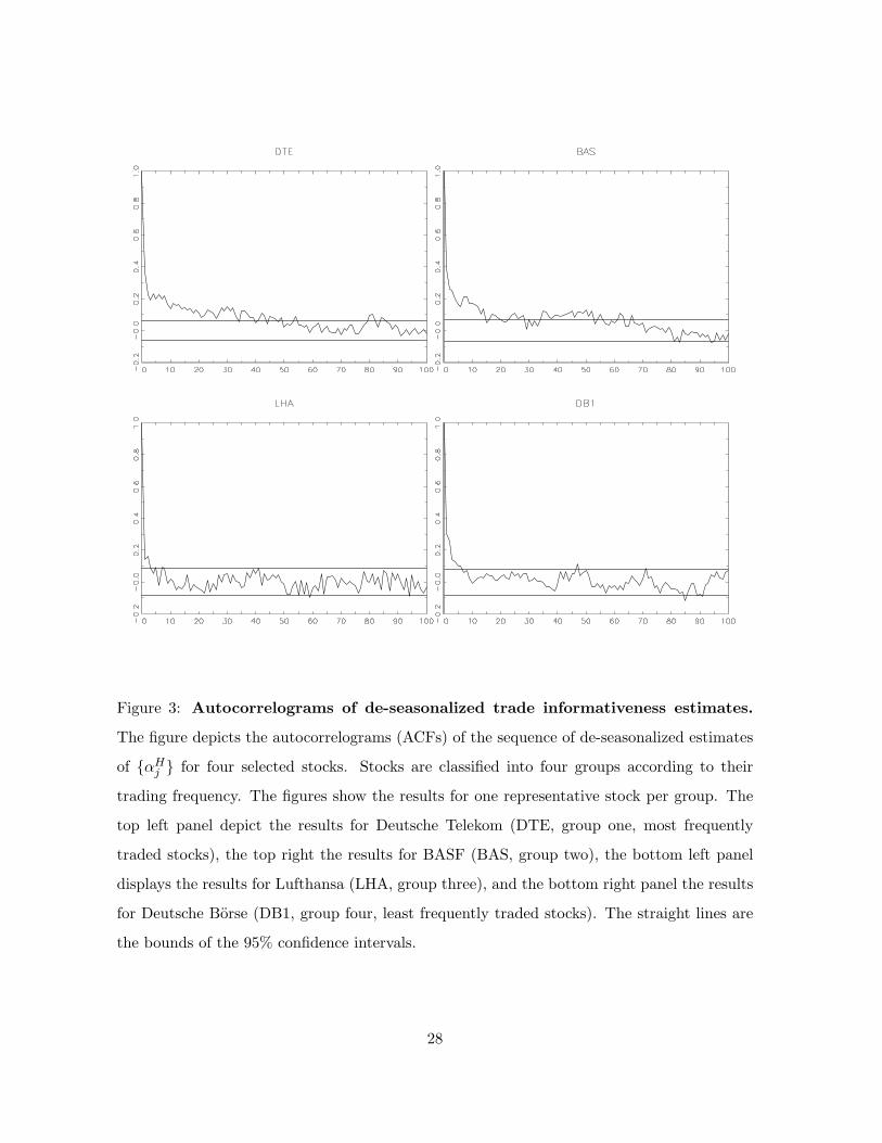
Figure 3: Autocorrelograms of de-seasonalized trade informativeness estimates.
The figure depicts the autocorrelograms (ACFs) of the sequence of de-seasonalized estimates
of {αHj } for four selected stocks. Stocks are classified into four groups according to their
trading frequency. The figures show the results for one representative stock per group. The
top left panel depict the results for Deutsche Telekom (DTE, group one, most frequently
traded stocks), the top right the results for BASF (BAS, group two), the bottom left panel
displays the results for Lufthansa (LHA, group three), and the bottom right panel the results
for Deutsche Borse (DB1, group four, least frequently traded stocks). The straight lines are
the bounds of the 95% confidence intervals.
28
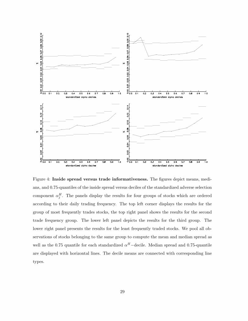
Figure 4: Inside spread versus trade informativeness. The figures depict means, medi-
ans, and 0.75-quantiles of the inside spread versus deciles of the standardized adverse selection
component αHj . The panels display the results for four groups of stocks which are ordered
according to their daily trading frequency. The top left corner displays the results for the
group of most frequently trades stocks, the top right panel shows the results for the second
trade frequency group. The lower left panel depicts the results for the third group. The
lower right panel presents the results for the least frequently traded stocks. We pool all ob-
servations of stocks belonging to the same group to compute the mean and median spread as
well as the 0.75 quantile for each standardized αH−decile. Median spread and 0.75-quantile
are displayed with horizontal lines. The decile means are connected with corresponding line
types.
29

Figure 5: Book liquidity beyond the best quotes (sell side) versus trade informa-
tiveness. The figures depict means, medians, and 0.75-quantiles of ask price impacts apt(v)
versus deciles of the standardized adverse selection component αHj . The panels display the
results for four groups of stocks which are ordered according to their daily trading frequency.
The top left corner displays the results for the group of most frequently trades stocks, the
top right panel shows the results for the second trade frequency group. The lower left panel
depicts the results for the third group. The lower right panel presents the results for the least
frequently traded stocks. We pool all observations of stocks belonging to the same group
to compute the mean and median price impacts as well as the 0.75 quantiles for each stan-
dardized αH−decile. The dashed lines correspond to the v =50,000 price impact and the
solid lines to the v =250,000 euro price impact. Median and 0.75-quantile price impacts are
displayed with horizontal lines. The decile means for each price impact are connected with
corresponding line types.
30
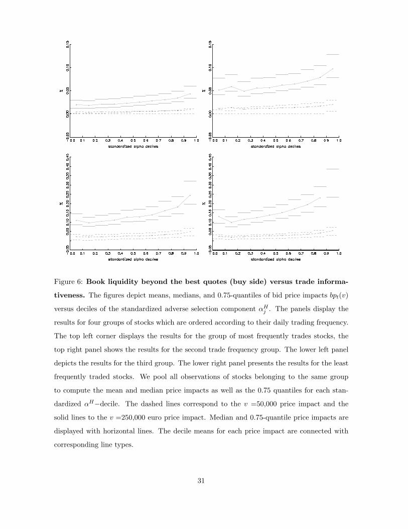
Figure 6: Book liquidity beyond the best quotes (buy side) versus trade informa-
tiveness. The figures depict means, medians, and 0.75-quantiles of bid price impacts bpt(v)
versus deciles of the standardized adverse selection component αHj . The panels display the
results for four groups of stocks which are ordered according to their daily trading frequency.
The top left corner displays the results for the group of most frequently trades stocks, the
top right panel shows the results for the second trade frequency group. The lower left panel
depicts the results for the third group. The lower right panel presents the results for the least
frequently traded stocks. We pool all observations of stocks belonging to the same group
to compute the mean and median price impacts as well as the 0.75 quantiles for each stan-
dardized αH−decile. The dashed lines correspond to the v =50,000 price impact and the
solid lines to the v =250,000 euro price impact. Median and 0.75-quantile price impacts are
displayed with horizontal lines. The decile means for each price impact are connected with
corresponding line types.
31

Figure 7: Trade size versus trade informativeness. The figures depict means, medians,
and 0.75-quantiles of the trading volume (in euros) versus deciles of the standardized adverse
selection component αHj . The panels display the results for four groups of stocks which are
ordered according to their daily trading frequency. The top left corner displays the results for
the group of most frequently trades stocks, the top right panel shows the results for the second
trade frequency group. The lower left panel depicts the results for the third group. The lower
right panel presents the results for the least frequently traded stocks. We pool all observations
of stocks belonging to the same group to compute the mean and median volume as well as the
0.75 quantile for the respective standardized αH−decile. Median volume and 0.75-quantile
are displayed with horizontal lines. The decile means are connected with corresponding line
types.
32

Figure 8: Trade duration versus trade informativeness. The figures depict means,
medians, and 0.75-quantiles of the trade durations (in seconds) versus deciles of the stan-
dardized adverse selection component αHj . The panels display the results for four groups of
stocks which are ordered according to their daily trading frequency. The top left corner dis-
plays the results for the group of most frequently trades stocks, the top right panel shows the
results for the second trade frequency group. The lower left panel depicts the results for the
third group. The lower right panel presents the results for the least frequently traded stocks.
We pool all observations of stocks belonging to the same group to compute the trade duration
mean, median and 0.75 quantile of the respective standardized αH−decile. Median duration
and 0.75-quantile are displayed with horizontal lines. The decile means are connected with
corresponding line types.
33