Understanding the Korean and Thai currency crises Reserve Bank of Chicago 45 Understanding the Korean and Thai currency crises Craig Burnside, Martin Eichenbaum, and Sergio Rebelo

45Federal Reserve Bank of Chicago

Understanding the Korean and Thai currency crises

Craig Burnside, Martin Eichenbaum, and Sergio Rebelo

Craig Burnside is a senior economist at the World Bank.Martin Eichenbaum is a professor of economics atNorthwestern University, a research associate of theNational Bureau of Economic Research (NBER), and aconsultant to the Federal Reserve Bank of Chicago.Sergio Rebelo is a professor of economics at NorthwesternUniversity and a research associate of the NBER.

Introduction and summary

In late 1997, Southeast Asia was rocked by bankingand currency crises. While dramatic in scope and in-tensity, this episode was only the latest in a seriesof �twin crises.� Other prominent examples includeArgentina (1980), Chile (1981), Uruguay (1981),Finland (1991), Sweden (1991), and Mexico (1994).In this article, we review and interpret the recentKorean and Thai experiences, focusing on the pivotalrole of unfunded contingent government liabilities.We concentrate on the Korean and Thai cases bothbecause their crises were severe and because neithercountry appeared to be a likely candidate for a currencycrisis, at least not from the perspective of standardeconomic models.

In addition to being of independent interest, thelessons learned from the Korean and Thai episodesshould be useful in predicting and averting future twincrises.1 In a nutshell, these lessons are as follows.First, twin crises are likely to erupt in countries whosegovernments have large prospective deficits stemmingfrom guarantees to failing financial sectors. Suchguarantees typically insure creditors�both domesticand foreign�against realizing large losses when finan-cial institutions that they have lent money to becomeinsolvent or go broke. Second, past deficits are, atbest, a noisy indicator of how large a government�sprospective deficits are. Accurately measuring thelatter requires a careful analysis of the nature of a gov-ernment�s guarantees and the probability that thoseguarantees will be called upon. It may never be pos-sible to predict precisely when a twin crisis will occur.But more accurate measures of prospective deficitsare likely to be helpful in predicting where twin criseswill occur. Finally, to avoid currency crises, govern-ments must have credible plans to finance contingentliabilities with credible, explicit fiscal reforms. Suchreforms include concrete measures to cut governmentexpenditures or raise taxes.

In the body of the article, we provide the empiricalbackground for our analysis. We begin by motivatingempirically the importance of past banking crises asa source of government liabilities. We then briefly re-view the salient features of the recent crises in Koreaand Thailand. These can be summarized as follows.

1. Both currency crises were difficult to predict onthe basis of standard economic indicators, suchas inflation rates, monetary growth rates, or pastgovernment deficits.

2. Neither banking crisis was difficult to anticipate,certainly not if one used publicly available infor-mation about the market value of financial firmsin Korea and Thailand.

3. When the crises came, they came with a vengeance.The Korean won and Thai baht rapidly depreciatedby over 50 percent and 80 percent, respectively,vis-à-vis the dollar before partially rebounding invalue. In addition to the large social costs associ-ated with severe recessions, the crises saddled theKorean and Thai governments with very large lia-bilities. These arose both from their implicit guar-antees and the need to restructure their respectivebanking systems. As we discuss below, these costsare now estimated to exceed 25 percent of Korea�sand Thailand�s gross domestic product (GDP).

4. After the crises, the rates of inflation and moneygrowth rose in both countries, though not by nearlyas much as the rates of depreciation of the won and

46 Economic Perspectives

the baht. The rise in the price of tradable goods wasmuch larger than the rise in the price of nontrad-able goods.

Later, we provide an explanation of the way inwhich prospective deficits could have caused the cur-rency crises. The basic idea is that the Korean and Thaifinancial sectors were in trouble prior to the currencycrises and investors knew this. Given the Korean andThai governments� implicit guarantees to their bank-ing sectors, market participants revised upwards theirestimates of future government deficits. Given thedifficulty of raising tax revenues or lowering govern-ment expenditures in the wake of a severe bankingcrisis, private agents expected that future deficits wouldbe financed, at least in part, by higher seignioragerevenues. This led to expectations of higher future in-flation rates and a reduction in the demand for domes-tic currency. The resulting drain on official reservesof foreign currency triggered the currency crises.Finally, because many financial institutions did nothedge the currency mismatch in their assets and lia-bilities, the currency crises exacerbated the initialbanking crises and raised the associated fiscal costs.

We articulate these ideas using a simplified versionof the model in Burnside, Eichenbaum, and Rebelo(1999). In versions of the model roughly calibratedto Korean data, a speculative attack occurs after theinformation about higher future deficits arrives butbefore the new monetary policy is implemented. Sothe model is consistent with the idea that the fixedexchange rate regimes in Korea and Thailand collapsedafter agents understood that the banks were failing,but before governments actually started to monetizetheir deficits. Thus the model can account for facts 1and 2 discussed above: The banking crises were pre-dictable but standard indicators of bad governmentpolicy�high deficits, high inflation rates, and rapidmoney growth�were not observed prior to the crises.

While successful on a number of important dimen-sions, the benchmark model suffers from severalshortcomings. First, it implies a larger rate of inflationthan actually occurred after the crises. Second, themodel predicts that the domestic Consumer Price Index(CPI) moves one to one with the exchange rate. So itinconsistent with the fact that the rise in measuredinflation was smaller than the rate of depreciation inthe won and baht. In addition, since the benchmarkmodel assumes that all goods are tradable, it cannotaddress the post crises differential rates of inflationin traded and nontraded good prices. We briefly dis-cuss ongoing research that shows how the benchmarkmodel can be modified to overcome these shortcom-ings.2 From the perspective of this article, the key

point is that the modifications do not alter the model�smessage about the connection between prospectivedeficits and currency crises.

Finally, we turn to the issue of which countriesmight be at risk for the kind of twin crises experiencedby Korea and Thailand. Here we reproduce and dis-cuss Standard and Poor�s recent estimates of govern-ments� contingent liabilities to financial sectors. Theseestimates reveal that a government�s exposure to futurecontingent liabilities is not well estimated by conven-tional debt measures. Since future deficits can be justas important as past deficits in triggering currencycrises, policymakers who focus only on conventionaldebt measures do so at their peril. When the stormcomes, they will be taken by surprise. Our researchsuggests that they need not be, provided that theyspend more resources on measuring the extent of theircontingent liabilities.

Basic facts

Our analysis of recent events in Southeast Asialeans heavily on the notion that the Thai and Koreangovernments faced serious fiscal problems becauseof implicit, unbudgeted guarantees to their bankingsectors. In this section we accomplish two tasks. First,we provide some evidence on the fiscal implicationsof banking crises in a variety of countries. Second,we briefly review the twin crises and their aftermathin Korea and Thailand.

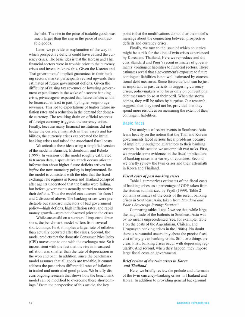
Fiscal costs of past banking crisesTable 1 summarizes estimates of the fiscal costs

of banking crises, as a percentage of GDP, taken fromthe studies summarized by Frydl (1999). Table 2contains estimates of the costs of the recent bankingcrises in Southeast Asia, taken from Standard andPoor�s Sovereign Ratings Service.3

Comparing tables 1 and 2 we see that, while large,the magnitude of the bailouts in Southeast Asia wasby no means unprecedented (see, for example, table1 on the costs of the Argentinian, Chilean, andUruguayan banking crises in the 1980s). No doubtthere is substantial uncertainty about the precise fiscalcost of any given banking crisis. Still, two things areclear. First, banking crises occur with depressing reg-ularity. And second, when they happen, they imposelarge fiscal costs on governments.

Brief review of the twin crises in Korea and Thailand

Here, we briefly review the prelude and aftermathof the twin currency�banking crises in Thailand andKorea. In addition to providing general background


for our analysis, we substantiate the claims summarizedas facts 1 through 4 in the introduction.

The currency crisesFigures 1 and 2 display the exchange rates of the

baht and the won, where the exchange rate is defined

as the price of a dollar in units of local currency.4 It isevident that Thailand and Korea experienced severecurrency crises in the latter part of 1997. The criseswere severe in the sense that both currencies underwentvery large depreciations in a short period of time: The

TABLE 1

Fiscal cost of banking crises, studies surveyed by Frydl (1999)

Caprio and Klingebiela Lindgren et al.b Dziobek & Pazarbasiogluc

(July 1996) (mid-1996) (December 1997)

Group Country Period Costd Period Costd Year Costd

Africa Benin 1988–90 17 1988Cote d’Ivoire 1988–91 25 1988–90 1991 13Ghana 1982–89 6 1983–89 3 1989 6Guinea 1985 3 1980–85Mauritania 1984–93 15 1991–93 1993 15Senegal 1988–91 17 1983–88Tanzania 1987 10 1988– 6.5 1992 14Zambia 1995 1.4 1994 3 1995 3

Asia Bangladesh Late 1980s– 1980s 4.5Indonesia 1994 1.8 1992– 2 1994 2Malaysia 1985–88 4.7 1985–88 4.7Philippines 1981–87 3 1981–87 13.2 1984 4Sri Lanka 1989–93 5 early 1990sThailand 1983–87 1.5 1983–87

Latin America Argentina 1980–82 55.3 1980–82 4Argentina 1995 1995 1994 0.3Bolivia 1994– 4.2Brazil 1994–95 7.5 1994–Chile 1981–83 41.2 1981–87 29 1983 33Colombia 1982–87 5 1982–85Mexico 1995 13.5 1994– 6.5 1994 13.5Peru 1983–90 1991 0.4Uruguay 1981–84 31.2Venezuela 1994–95 18 1994– 17 1994 17

Mideast and Israel 1977–83 30 1983–84North Africa Kuwait 1980s Mid-1980s 1992 45

Turkey 1982–85 2.5 1982Turkey 1994 1

Transition Bulgaria 1990s 14 1991–economies Czech Rep. 1991– 12

Estonia 1992 1.4 1992–95 1.8Hungary 1991–95 10 1987– 9 1993 12.2Kazakhstan 1991–95 4.5 1995Poland 1990s $1.7bil 1991– 1993 5.7Slovenia 1990s $1.3bil 1992–94

Advanced Finland 1991–93 8 1991–94 8.4 1991 9.9OECD France 1994–95 $10bil 1991–95 0.6

Japan 1990s $100bil 1992 1995Norway 1967–89 4 1987–93 3.3Spain 1977–85 16.8 1977–85 5.6 1980 15Sweden 1991 6.4 1990–93 4 1991 4.3United States 1984–91 3.2 1980–92 2.4

aDates indicate the period of the crisis episode. Dash indicates that the crisis was ongoing at the date of publication.bDates indicate the period of the banking sector difficulties. Dash indicates that the difficulties were ongoing atthe date of publication.cDate indicates year of onset of restructuring action.dPercent of GDP, unless stated otherwise.Note: OECD is Organization for Economic Cooperation and Development.


value of the baht relative to the dollar declined byover 50 percent between June 1997 and January1998; and the value of the won relative to the dollardeclined by over 48 percent between October 1997and January 1998.5

The banking�financial sector crisesBoth Korea and Thailand experienced severe

banking�financial sector crises that began before theircurrency crises. Corsetti, Pesenti, and Roubini (1999)report that pre-crisis nonperforming loan rates were19 percent in Thailand and 16 percent in Korea, orroughly 30 percent and 22 percent of GDP, respec-tively. That being said, the currency crises certainlyexacerbated the financial crises.6 According to J.P.Morgan (1998), as of June 1998, the rate of nonper-forming loans in both Korea and Thailand had risen

to roughly 30 percent. By June 1999, the cost of re-capitalizing and restructuring the banking system inThailand reached 35 percent of GDP (see table 2). Asof December 1999, the corresponding cost in Koreahad reached 24 percent of GDP.

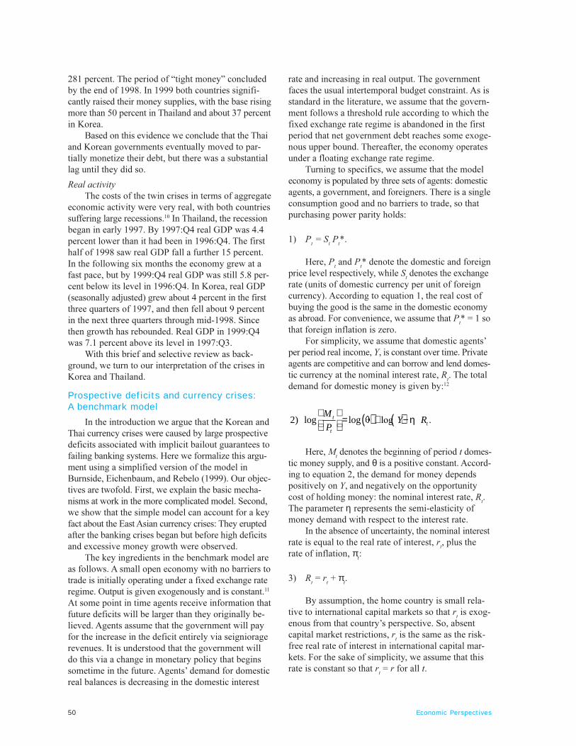
Was the public aware of the banking crises be-fore the currency crises? In our view the answer isyes. First, proprietary information from some bankrating services and investment banks had raised doubtsabout the health of the local banks. Second, the mar-ket value of the banking and financial sectors inThailand and Korea declined precipitously before thecurrency crisis hit. Table 3, extracted from Burnside,Eichenbaum, and Rebelo (1999), reports indexes ofthe stock market value of publicly traded banks andfinancial firms in Thailand and Korea. In addition, wereport the analog value of the commercial and manu-facturing sector in Thailand and Korea, respectively.7

The column labeled �Pre-crisis peak� pertains to thedate of the peak value of the banking sector in the twocountries. Three features of table 3 are worth noting.First, in both countries, the value of the banking andfinance sectors fell by large amounts before the cur-rency crises. For example, in the period between thepre-crisis banking peak and the day immediately pri-or to the currency crisis, the value of the Thai andKorean finance sectors fell by 92 percent and 52 per-cent, respectively. Second, in the case of Thailand,the value of the financial sector fell by a large amountrelative to the decline in the commerce sector. In thecase of Korea, the manufacturing sector index actuallyrose up to the day before the crisis. So the decline in

the value of the financial sectors did notsimply reflect a decline in the overallstock market. Markets seemed particular-ly concerned about the financial sector.

Both Thailand and Korea had lowinflation rates prior to their currency cri-ses. Over the two previous years, the CPIin Thailand and Korea rose at annualrates of 5 percent and 4.6 percent, respec-tively,8 giving no hint of the currency cri-ses to come.

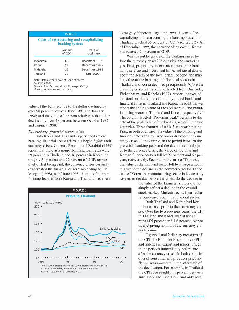
Figures 1 and 2 display measures ofthe CPI, the Producer Price Index (PPI),and indexes of export and import pricesin the periods immediately before andafter the currency crises. In both countriesoverall consumer and producer price in-flation was moderate in the aftermath ofthe devaluation. For example, in Thailand,the CPI rose roughly 11 percent betweenJune 1997 and June 1998, and only rose

TABLE 2

Costs of restructuring and recapitalizingbanking system

Percent Date ofof GDP estimate

Indonesia 65 November 1999

Korea 24 December 1999

Malaysia 22 December 1999

Thailand 35 June 1999

Note: Dates refer to date of issue of sourcecountry reports.Source: Standard and Poor’s Sovereign RatingsService, various country reports.

FIGURE 1

Prices in Thailand

index, June 1997=100

Baht/U.S. dollar

Notes: IUV is import unit value; EUV is export unit value; PPI isProducer Price Index; and CPI is Consumer Price Index.Source: “Data bank” at www.bot.or.th.

IUVEUV PPI

CPI


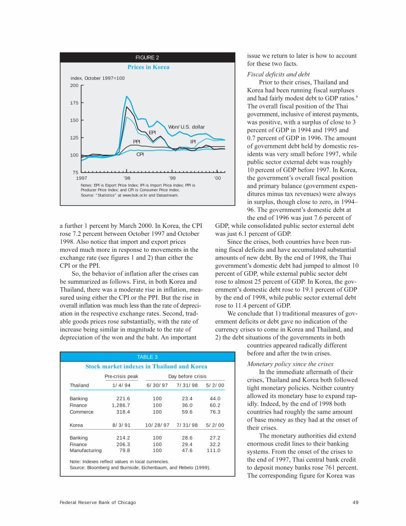
a further 1 percent by March 2000. In Korea, the CPIrose 7.2 percent between October 1997 and October1998. Also notice that import and export pricesmoved much more in response to movements in theexchange rate (see figures 1 and 2) than either theCPI or the PPI.

So, the behavior of inflation after the crises canbe summarized as follows. First, in both Korea andThailand, there was a moderate rise in inflation, mea-sured using either the CPI or the PPI. But the rise inoverall inflation was much less than the rate of depreci-ation in the respective exchange rates. Second, trad-able goods prices rose substantially, with the rate ofincrease being similar in magnitude to the rate ofdepreciation of the won and the baht. An important

issue we return to later is how to accountfor these two facts.

Fiscal deficits and debtPrior to their crises, Thailand and

Korea had been running fiscal surplusesand had fairly modest debt to GDP ratios.9

The overall fiscal position of the Thaigovernment, inclusive of interest payments,was positive, with a surplus of close to 3percent of GDP in 1994 and 1995 and0.7 percent of GDP in 1996. The amountof government debt held by domestic res-idents was very small before 1997, whilepublic sector external debt was roughly10 percent of GDP before 1997. In Korea,the government�s overall fiscal positionand primary balance (government expen-ditures minus tax revenues) were alwaysin surplus, though close to zero, in 1994�96. The government�s domestic debt atthe end of 1996 was just 7.6 percent of

GDP, while consolidated public sector external debtwas just 6.1 percent of GDP.

Since the crises, both countries have been run-ning fiscal deficits and have accumulated substantialamounts of new debt. By the end of 1998, the Thaigovernment�s domestic debt had jumped to almost 10percent of GDP, while external public sector debtrose to almost 25 percent of GDP. In Korea, the gov-ernment�s domestic debt rose to 19.1 percent of GDPby the end of 1998, while public sector external debtrose to 11.4 percent of GDP.

We conclude that 1) traditional measures of gov-ernment deficits or debt gave no indication of thecurrency crises to come in Korea and Thailand, and2) the debt situations of the governments in both

countries appeared radically differentbefore and after the twin crises.

Monetary policy since the crisesIn the immediate aftermath of their

crises, Thailand and Korea both followedtight monetary policies. Neither countryallowed its monetary base to expand rap-idly. Indeed, by the end of 1998 bothcountries had roughly the same amountof base money as they had at the onset oftheir crises.

The monetary authorities did extendenormous credit lines to their bankingsystems. From the onset of the crises tothe end of 1997, Thai central bank creditto deposit money banks rose 761 percent.The corresponding figure for Korea was

FIGURE 2

Prices in Korea

index, October 1997=100

Won/U.S. dollar

Notes: EPI is Export Price Index; IPI is Import Price Index; PPI isProducer Price Index; and CPI is Consumer Price Index.Source: “Statistics” at www.bok.or.kr and Datastream.

IPIPPI

CPI

TABLE 3

Stock market indexes in Thailand and Korea

Pre-crisis peak Day before crisis

Thailand 1/4/94 6/30/97 7/31/98 5/2/00

Banking 221.6 100 23.4 44.0Finance 1,286.7 100 36.0 60.2Commerce 318.4 100 59.6 76.3

Korea 8/3/91 10/28/97 7/31/98 5/2/00

Banking 214.2 100 28.6 27.2Finance 206.3 100 29.4 32.2Manufacturing 79.8 100 47.6 111.0

Note: Indexes reflect values in local currencies.Source: Bloomberg and Burnside, Eichenbaum, and Rebelo (1999).

EPI


281 percent. The period of �tight money� concludedby the end of 1998. In 1999 both countries signifi-cantly raised their money supplies, with the base risingmore than 50 percent in Thailand and about 37 percentin Korea.

Based on this evidence we conclude that the Thaiand Korean governments eventually moved to par-tially monetize their debt, but there was a substantiallag until they did so.

Real activityThe costs of the twin crises in terms of aggregate

economic activity were very real, with both countriessuffering large recessions.10 In Thailand, the recessionbegan in early 1997. By 1997:Q4 real GDP was 4.4percent lower than it had been in 1996:Q4. The firsthalf of 1998 saw real GDP fall a further 15 percent.In the following six months the economy grew at afast pace, but by 1999:Q4 real GDP was still 5.8 per-cent below its level in 1996:Q4. In Korea, real GDP(seasonally adjusted) grew about 4 percent in the firstthree quarters of 1997, and then fell about 9 percentin the next three quarters through mid-1998. Sincethen growth has rebounded. Real GDP in 1999:Q4was 7.1 percent above its level in 1997:Q3.

With this brief and selective review as back-ground, we turn to our interpretation of the crises inKorea and Thailand.

Prospective deficits and currency crises:A benchmark model

In the introduction we argue that the Korean andThai currency crises were caused by large prospectivedeficits associated with implicit bailout guarantees tofailing banking systems. Here we formalize this argu-ment using a simplified version of the model inBurnside, Eichenbaum, and Rebelo (1999). Our objec-tives are twofold. First, we explain the basic mecha-nisms at work in the more complicated model. Second,we show that the simple model can account for a keyfact about the East Asian currency crises: They eruptedafter the banking crises began but before high deficitsand excessive money growth were observed.

The key ingredients in the benchmark model areas follows. A small open economy with no barriers totrade is initially operating under a fixed exchange rateregime. Output is given exogenously and is constant.11

At some point in time agents receive information thatfuture deficits will be larger than they originally be-lieved. Agents assume that the government will payfor the increase in the deficit entirely via seignioragerevenues. It is understood that the government willdo this via a change in monetary policy that beginssometime in the future. Agents� demand for domesticreal balances is decreasing in the domestic interest

rate and increasing in real output. The governmentfaces the usual intertemporal budget constraint. As isstandard in the literature, we assume that the govern-ment follows a threshold rule according to which thefixed exchange rate regime is abandoned in the firstperiod that net government debt reaches some exoge-nous upper bound. Thereafter, the economy operatesunder a floating exchange rate regime.

Turning to specifics, we assume that the modeleconomy is populated by three sets of agents: domesticagents, a government, and foreigners. There is a singleconsumption good and no barriers to trade, so thatpurchasing power parity holds:

1) Pt = S

t P

t*.

Here, Pt and P

t* denote the domestic and foreign

price level respectively, while St denotes the exchange

rate (units of domestic currency per unit of foreigncurrency). According to equation 1, the real cost ofbuying the good is the same in the domestic economyas abroad. For convenience, we assume that P

t* = 1 so

that foreign inflation is zero.For simplicity, we assume that domestic agents�

per period real income, Y, is constant over time. Privateagents are competitive and can borrow and lend domes-tic currency at the nominal interest rate, R

t. The total

demand for domestic money is given by:12

( ) ( )2) log log ORJ �

= + − η t

tt

MY R

P

Here, Mt denotes the beginning of period t domes-

tic money supply, and θ is a positive constant. Accord-ing to equation 2, the demand for money dependspositively on Y, and negatively on the opportunitycost of holding money: the nominal interest rate, R

t.

The parameter η represents the semi-elasticity ofmoney demand with respect to the interest rate.

In the absence of uncertainty, the nominal interestrate is equal to the real rate of interest, r

t, plus the

rate of inflation, πt:

3) Rt = r

t + π

t.

By assumption, the home country is small rela-tive to international capital markets so that r

t is exog-

enous from that country�s perspective. So, absentcapital market restrictions, r

t is the same as the risk-

free real rate of interest in international capital mar-kets. For the sake of simplicity, we assume that thisrate is constant so that r

t = r for all t.


The government of the home country purchasesgoods, g

t, makes transfer payments, v

t, levies lump sum

taxes, τt, and can borrow at the real interest rate r.

Again, for simplicity, we assume that gt, v

t, and τ

t are

constant over time and equal to g, v, and τ, respectively.

A sustainable fixed exchange rate regimeSuppose that the home country is initially in a

fixed exchange rate regime so that St = S. Equation 1

implies that the domestic rate of inflation, πt, is equal

to the foreign rate of inflation, πt*, which we assume

equals zero. It follows from equation 3 that the nomi-nal rate of interest is equal to the constant real inter-est rate: R

t = r for all t ≥ 0. Under a fixed exchange

rate, the domestic money supply is endogenous: Itmust equal the level of money demanded, given theexchange rate, S,

4) M = SθY exp(�ηr).

If the government tried to print more money thanM, private agents would simply trade it, at the fixedexchange rate, for foreign reserves. Consequently, aslong as the country is in a fixed exchange rate regime,the government cannot generate seigniorage revenues.13

Under what circumstances is the fixed exchangerate regime sustainable? In our model the answer tothis question reduces to whether the money supplycan be constant over time. Whether this is possibledepends critically on whether the government canabstain from raising seigniorage revenues. This in turndepends on the government�s fiscal policy.

To see the nature of the required restrictions onfiscal policy, note that with money constant for all t,the government�s flow budget constraint is:

5) .= + + − τ&t tb rb g v

Here, bt represents the government�s stock of

real debt, net of any assets, and tb& denotes the deriva-tive of b

t with respect to time. According to equation

5, the change in bt (more precisely, )&

tb is equal to theinterest cost of servicing government debt, rb

t, plus

the primary deficit, g + v � t. Imposing the conditionthat the present value of b

t goes to zero in the infinite

future, we obtain the government�s intertemporalbudget constraint,14

6) rb0 = τ � g � v.

According to equation 6, for the fixed exchangerate to be sustainable, the government surplus must bejust large enough to cover the interest cost of servicing

its initial debt. When this is the case, the governmentdoes not print money. It simply stands ready to tradedomestic money for foreign money at the exchangerate S. Since the demand for money is constant, sotoo is the supply. So, as long as equation 6 holds, theeconomy will be in a sustainable fixed exchange rateequilibrium with S

t = S for all t.

A currency crisisTo see how a banking crisis can generate a cur-

rency crisis, suppose that equation 6 initially holds.Then, at time t = 0, private agents learn that there hasbeen an increase in the present value of the deficitequal to φ, say because of an increase in future trans-fer payments associated with bank bailouts. Also,suppose private agents correctly believe that the gov-ernment will not undertake a fiscal reform to pay forthe bank bailouts; that is, they will not raise taxes orlower real government purchases or transfers. Whilewe could allow for a partial fiscal reform, for simplicitywe assume that g, v, and τ remain constant at theirinitial pre-crisis values.15 It follows that the only waythat the government can satisfy its intertemporal bud-get constraint is to embark on a monetary policy thatgenerates a present value of seigniorage revenuesequal to φ:16

*( ) .rt rit i

tit i

M MPV Seigniorage e dt e

P P

∞ − −∆7) φ = = + ∑∫

&

Here, t* denotes the time when the economymoves to a floating exchange rate regime, tM& is thederivative of the money supply with respect to time,

and *

rtt

tt

Me dt

P

∞ −∫&

represents the present value of the

resources that the government raises by printing

money. The term rii

ii

Me

P−∆∑ represents changes in

seigniorage revenue following discrete jumps in themoney supply. These terms must be included becausethe money supply may jump discontinuously whenthe fixed exchange rate regime collapses or becauseof government monetary policy (see Burnside,Eichenbaum, and Rebelo, 1999 and 2000a).

Could the fixed exchange rate be sustained oncenew information about higher deficits arrives? Suppose,for a moment, that it could. Then the money supplywould never change and the government could notcollect any seigniorage revenues. So all the terms onthe right-hand side of equation 7 would equal zero.But then the government�s budget constraint wouldnot hold. This contradicts the assumption that thefixed exchange rate regime is sustainable. We concludethat the government must at some point move to a


floating exchange rate system. The precise time atwhich this occurs depends on 1) the government�srule for abandoning fixed exchange rates, and 2) thegovernment�s new monetary policy.

With respect to 1, we follow a standard assump-tion in the literature that the government abandonsthe fixed exchange rate regime according to a thresh-old rule on government debt.17 Specifically, we assumethat the government floats the currency in the firsttime instance, t*, when its net debt hits some finiteupper bound. As it turns out, this is equivalent toabandoning the fixed exchange rate whenever theamount of domestic money sold by private agents inexchange for foreign reserves exceeds χ percent ofthe initial money supply (see the appendix). In addi-tion to being a good description of what happens inactual crises, the threshold rule assumption can be in-terpreted as a short-run borrowing constraint on thegovernment: It limits how much reserves the govern-ment can borrow to defend the fixed exchange rate.18

With respect to 2, we assume that at some pointin the future, time T, the government will engineer adiscrete increase in the money supply of γ percentrelative to M, the level of the money supply duringthe fixed exchange rate regime. In addition it will setthe growth rate of the money supply from then onequal to µ. The parameters µ and γ must be such thatthe government�s intertemporal budget constraint,equation 7, holds. This specification decouples theendogenous timing of the speculative attack from thetime at which the government undertakes its newmonetary policy. Because of this we can allow fora delay between the end of the fixed exchange rateregime and when the government moves to monetizethe debt.

Before turning to the quantitative properties ofour model, we note that the rate of inflation, themoney supply, and the level of government debt canbe discontinuous in our perfect foresight economy.However, the exchange rate path must be continuous.To see why, suppose to the contrary that there was adiscontinuous increase in the exchange rate at timet*. Since purchasing power parity implies that P

t = S

t,

inflation would be infinity at t*. This would implythat the nominal interest rate would also be infinityat t* so that money demand would be equal to zero.Private agents would want to sell all of the domesticmoney supply to the government. But the governmentis only willing to buy χ percent of it. Hence, this can-not be an equilibrium.

Equilibrium of the model: Numerical examplesIn the appendix, we show how to solve for the

equilibrium of the model economy. Here, we describe

the characteristics of the equilibrium for a calibratedversion of the model.

■ We normalize real income, Y, and the initialexchange rate, S, to 1.

■ We set the parameter φ to 0.25, a conservativeestimate of the cost of Korea�s banking crisisrelative to its GDP.

■ We set the semi-elasticity of money demand withrespect to the interest rate, η, equal to 0.5. This isconsistent with the range of estimates of moneydemand elasticities in developing countries pro-vided by Easterly, Mauro, and Schmidt-Hebbel(1985). Since Korea is not included in that study,we discuss the sensitivity of our results to thisparameter.

■ We assume that the risk-free real interest rate, r, isequal to 1 percent and set the constant, θ, in mon-ey demand so that the model is consistent with theratio of real balances to GDP in Korea before thecrisis. See Burnside, Eichenbaum, and Rebelo(1999, 2000a). For η = 0.05, this implies a valueof θ approximately equal to 0.06.

■ Based on the evidence in Burnside, Eichenbaum,and Rebelo (1999), we set the threshold parameter,χ, to 0.03.

■ For simplicity we normalize the government�sinitial stock of debt, b

0, to zero.

■ The monetary base in Korea was roughly the sameat the end of 1998 as at the beginning of the crisis.However, by the end of 1999, the base had risen byover 30 percent. Given these facts, the key questionin deciding on a value for T is: When did agents be-come convinced that the government would have tobail the banks out? This is a difficult issue to resolve.Here we report results for T = 3. While our qualita-tive results are robust to this choice, we think furtherresearch on this question is important. At the endof this section we briefly consider one interestingimplication of setting T = 1.

■ We set the parameter γ to 0.1. Finally, we solvefor the value of µ that satisfies the government�sintertemporal budget constraint (µ= 0.043).

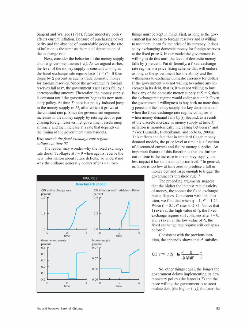
Figure 3 displays the equilibrium path of thebenchmark model. Two features are worth noting.First, the collapse of the fixed exchange rate regimetakes place at time t* = 2.19, after the new informa-tion about the deficit arrives (t = 0) but before the newmonetary policy is implemented (T = 3). Second,inflation begins to rise at t*, before the change in mon-etary policy. So, consistent with the classic results in


Sargent and Wallace (1981), future monetary policyaffects current inflation. Because of purchasing powerparity and the absence of nontradable goods, the rateof inflation is the same as the rate of depreciation ofthe exchange rate.

Next, consider the behavior of the money supplyand net government assets (�b

t). As we argued earlier,

the level of the money supply is constant as long asthe fixed exchange rate regime lasts ( t < t*). It thendrops by χ percent as agents trade domestic moneyfor foreign reserves. Since the government�s foreignreserves fall at t*, the government�s net assets fall by acorresponding amount. Thereafter, the money supplyis constant until the government begins its new mon-etary policy. At time T there is a policy-induced jumpin the money supply to M

T after which it grows at

the constant rate µ. Since the government engineersincreases in the money supply by retiring debt or pur-chasing foreign reserves, net government assets jumpat time T and then increase at a rate that depends onthe timing of the government bank bailouts.

Why doesn�t the fixed exchange rate regimecollapse at time 0?

The reader may wonder why the fixed exchangerate doesn�t collapse at t = 0 when agents receive thenew information about future deficits. To understandwhy the collapse generally occurs after t = 0, two

things must be kept in mind. First, as long as the gov-ernment has access to foreign reserves and is willingto use them, it can fix the price of its currency. It doesso by exchanging domestic money for foreign reservesat the fixed price S. In our model the government iswilling to do this until the level of domestic moneyfalls by χ percent. Put differently, a fixed exchangerate regime is a price fixing scheme that will endureas long as the government has the ability and thewillingness to exchange domestic currency for dollars.If the government was not willing to endure any in-creases in its debt, that is, it was not willing to buyback any of the domestic money supply at S

t = S, then

the exchange rate regime would collapse at t = 0. Giventhe government�s willingness to buy back no more thanχ percent of the money supply, the key determinant ofwhen the fixed exchange rate regime collapses iswhen money demand falls by χ. Second, as a resultof the discrete increase in money supply at time T,inflation is monotonically increasing between t* andT (see Burnside, Eichenbaum, and Rebelo, 2000a).This reflects the fact that in standard Cagan moneydemand models, the price level at time t is a functionof discounted current and future money supplies. Animportant feature of this function is that the furtherout in time is the increase in the money supply, theless impact it has on the initial price level.19 In general,inflation is too low at time zero to produce a fall in

money demand large enough to trigger thegovernment�s threshold rule.20

The preceding arguments suggestthat the higher the interest rate elasticityof money, the sooner the fixed exchangerate collapses. Consistent with this intu-ition, we find that when η = 1, t* = 1.24.When η = 0.1, t* rises to 2.85. Notice that1) even at the high value of η, the fixedexchange regime still collapses after t = 0,and 2) even at the low value of η, thefixed exchange rate regime still collapsesbefore T.

Consistent with the previous intu-ition, the appendix shows that t* satisfies:

* ln .t T χ

8) = + η χ + γ + µη

So, other things equal, the longer thegovernment delays implementing its newmonetary policy (the larger is T) and themore willing the government is to accu-mulate debt (the higher is χ), the later the

FIGURE 3

Benchmark model

percentCPI and exchange rate

percentCPI inflation and tradables inflation

percentMoney supply

percentGovernment assets

time time

time time


fixed exchange rate regime will collapse. In addition,the higher is the interest rate elasticity of money de-mand (the larger is η) and the more money the gov-ernment prints in the future (the higher are γ and µ),the sooner the speculative attack will occur.21

Some caution is required in interpreting these re-sults because we are not free to vary the parameterson the right-hand side of equation 8 independently ofeach other. For example, equation 8 indicates that t*is increasing in the threshold rule parameter, χ, takingthe parameters that control monetary policy (γ, µ,and T) as given. But these parameters must be adjust-ed whenever a different χ is considered because thegovernment�s intertemporal budget constraint musthold. This issue is addressed by Burnside, Eichenbaum,and Rebelo (1999), who show numerically that thequalitative conclusions emerging from equation 8remain intact even after the appropriate adjustmentsare made. This is also the case for the simple modelconsidered here. For example, if we set T to 1, thenwith one exception the equilibrium path of the modelis qualitatively similar to the one depicted in figure3. The exception is that t* falls to 0.18 or a bit overtwo months. Interestingly, this is the time lag betweenwhen forward premia on baht�dollar exchange ratesbegan to rise significantly and the Thai currencycrises occurred (see Burnside, Eichenbaum, andRebelo, 1999).

Strengths and weaknesses of the benchmark modelOn the positive side, the benchmark model does

what it was intended to do: It illustrates the fact thatnew information about prospective deficits can causethe collapse of a fixed exchange rate regime afterinformation about the deficit arrives but before thegovernment starts its new monetary policy. In addi-tion, the model reproduces the fact that CPI inflationinitially surges in the wake of the exchange rate col-lapse and then stabilizes at a lower level.22

On the negative side, 1) the model clearly over-states the actual rate of inflation in Korea after thecrises, particularly in the period between t* and T(see figure 2), and 2) the model does not account forthe different response in tradable and nontradablegoods prices. In assessing these shortcomings, it isimportant to note that the model�s implications forinflation depend heavily on two simplifying assump-tions. First, we assume that the only additional sourceof revenues available to the government in the after-math of the currency crisis is seigniorage. Second,there is only one good in the model economy, andpurchasing power parity holds. It follows from equation1 that an x percent rate of devaluation is necessarily

associated with an x percent rise in the price level.This is clearly counterfactual. In the next section, wediscuss work in Burnside, Eichenbaum, and Rebelo(1999, 2000a) that examines the implications ofrelaxing these assumptions.23

Perturbations to the benchmark model

Allowing for nonindexed government liabilitiesIn the benchmark model, we assume that all of

the government�s liabilities are perfectly indexed, sothat their real value is unaffected by a devaluation. Inreality, governments have liabilities denominated inunits of local currency that are not indexed to the rateof inflation. These liabilities are of two types: a) domes-tic bonds issued before information about a bankingcrisis becomes known, and b) obligations to programslike Social Security or commitments to purchase laborservices and other nontraded goods whose value ispreset in units of the domestic currency. Burnside,Eichenbaum, and Rebelo (1999, 2000a) discuss theimpact of these types of liabilities on the implicationsof the benchmark model.

The basic point is that inflation reduces the realvalue of nonindexed liabilities and acts like a partialfiscal reform, effectively providing the governmentwith a source of revenue other than seigniorage. Butto gain access to these revenue sources, there must beinflation. In our model, inflation is possible only in aflexible exchange rate regime. So the presence ofnonindexed liabilities does not allow the governmentto escape a currency crisis. However, it does allowthe government to print less money than it wouldhave to in the absence of nonindexed liabilities. Thisin turn implies that the modified model does a muchbetter job of accounting for the observed post-crisesrates of inflation in Korea and Thailand.24

Allowing for nontraded goodsThe benchmark model assumes that all goods

are tradable and that purchasing power parity holds.Because of this, it is inconsistent with two key factsabout the crises in Korea and Thailand: 1) the rateof CPI inflation was much lower than the rate ofdepreciation in the won and the baht, and 2) the priceof tradable goods rose much more than the price ofnontradable goods after the fixed exchange rateregimes collapsed.

In modifying the benchmark model we areforced to confront the question What underlies theempirical failure of purchasing power parity? In itssimplest form this condition asserts that the real costof buying the CPI basket of goods is the same in allcountries. In reality some goods simply aren�t traded,


so there is no reason for their prices to be the same indifferent countries. Consequently, the real price ofthe CPI basket will not be equalized across countries.Purchasing power parity may also fail because trans-portation and distribution costs prevent tradable goodprices from equalizing across countries.

Burstein, Neves, and Rebelo (2000) argue on em-pirical grounds that total distribution costs (includingwholesale and retail services, marketing, and so on)are often more significant than the costs of transport-ing goods across countries. They study the role playedby the distribution sector in shaping the behavior ofreal exchange rates during exchange rate based stabi-lizations. Burnside, Eichenbaum, and Rebelo (2000a)show how to use Burstein, Neves, and Rebelo�s anal-ysis to break the benchmark model�s counterfactuallytight link between the inflation rate and the rate ofdepreciation of the exchange rate. The key result isthat once some stickiness in nontraded goods pricesis allowed for, the modified model does a reasonablejob of accounting quantitatively for the differentpost-crisis responses of traded and nontraded goodsprices in Korea and Thailand.

The basic features of the modified model canbe described as follows. As in Burstein, Neves, andRebelo (2000), assume that it takes δ units of non-traded goods to distribute one unit of the traded goodto the domestic retail sector. Let P

tNT and P

tT denote

the time t price of a nontraded good and the time tprice of a traded good before distribution. Supposefor simplicity that the distribution and retail sectorsof the economy are perfectly competitive. Then theretail price of a traded good is equal to P

tT + δP

tNT.

The CPI is defined to be the geometric average of theprice of the nontraded good and the retail price of thetraded good:

( ) ( )1,

−ωω9) = + δT NT NTt t t tP P P P

where ω is a number between 0 and 1.The demand for real balances is given by equation

2, where Pt is given by equation 9. By assumption,

purchasing power parity holds for the price of tradedgoods, exclusive of distribution services. With P

t*

equal to 1, this implies PtT = S. Burnside, Eichenbaum,

and Rebelo (2000a) also allow for nominal rigiditiesin the price of nontradable goods. With these changes,the modified model is qualitatively consistent withfacts 1 and 2 above.

Much work remains to be done in assessing theempirical plausibility of the modified versions of thebenchmark model discussed in this section. Still, the

results in Burnside, Eichenbaum, and Rebelo (1999,2000a) suggest that these types of models are capableof explaining the large departures from purchasingpower parity and relatively low inflation rates ob-served in the wake of currency crises. Just as important,bringing the models into closer conformity with theseaspects of the data does not alter our basic message:Unfunded prospective deficits can be an importantsource of currency crises.

Prospective deficits: Other countries

Throughout this article, we examine the role ofunfunded prospective deficits as a potential cause ofcurrency crises. We are not alone in this view. At theend of 1997, Standard and Poor�s began to report esti-mates of contingent government liabilities stemmingfrom implicit guarantees to financial sectors. Next,we discuss these estimates and their relationship toconventional debt measures.

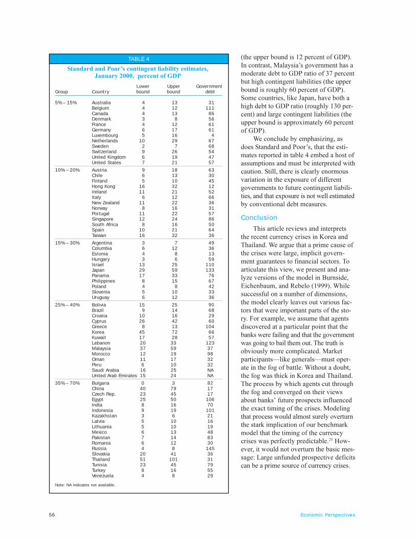
Table 4 reproduces Standard and Poor�s contingentgovernment liability estimates as of January 2000. Toarrive at these estimates, Standard and Poor�s first es-timates the lower and upper percentages of financialintermediaries� loans that are at risk under variousscenarios it deems to be likely. These are reported inthe column labeled �Group.� These bounds are mul-tiplied by a measure of the size of the financial systemrelative to GDP to generate estimates of lower andupper bounds for government contingent liabilities.These are reported in table 4 in the columns labeled�Lower bound� and �Upper bound.� Note that theseestimates can be large either because the financialsystem has substantial exposure to nonperformingloans or because a country�s banking system is largerelative to its GDP. The final column in table 4 sum-marizes the size of existing government debt relativeto GDP.

Two features of table 4 are worth noting. First,there is enormous variation in the size of governmentliabilities across different countries. The performanceof some countries on the low end like Denmark andCanada reflects very solid financial institutions, whilethe performance of countries like Bulgaria reflects thesmall size of their financial sector. At the high end,the performance of countries like Japan, Panama,Malaysia, China, the Czech Republic, Egypt, Korea,and Thailand reflects financial sectors that are bothlarge and risky.

Second, there is not a tight link between existinggovernment debt and contingent liabilities. For exam-ple, Belgium�s government has a very high debt toGDP ratio of 111 percent, but low contingent liabilities


(the upper bound is 12 percent of GDP).In contrast, Malaysia�s government has amoderate debt to GDP ratio of 37 percentbut high contingent liabilities (the upperbound is roughly 60 percent of GDP).Some countries, like Japan, have both ahigh debt to GDP ratio (roughly 130 per-cent) and large contingent liabilities (theupper bound is approximately 60 percentof GDP).

We conclude by emphasizing, asdoes Standard and Poor�s, that the esti-mates reported in table 4 embed a host ofassumptions and must be interpreted withcaution. Still, there is clearly enormousvariation in the exposure of differentgovernments to future contingent liabili-ties, and that exposure is not well estimatedby conventional debt measures.

Conclusion

This article reviews and interpretsthe recent currency crises in Korea andThailand. We argue that a prime cause ofthe crises were large, implicit govern-ment guarantees to financial sectors. Toarticulate this view, we present and ana-lyze versions of the model in Burnside,Eichenbaum, and Rebelo (1999). Whilesuccessful on a number of dimensions,the model clearly leaves out various fac-tors that were important parts of the sto-ry. For example, we assume that agentsdiscovered at a particular point that thebanks were failing and that the governmentwas going to bail them out. The truth isobviously more complicated. Marketparticipants�like generals�must oper-ate in the fog of battle. Without a doubt,the fog was thick in Korea and Thailand.The process by which agents cut throughthe fog and converged on their viewsabout banks� future prospects influencedthe exact timing of the crises. Modelingthat process would almost surely overturnthe stark implication of our benchmarkmodel that the timing of the currencycrises was perfectly predictable.25 How-ever, it would not overturn the basic mes-sage: Large unfunded prospective deficitscan be a prime source of currency crises.

TABLE 4

Lower Upper GovernmentGroup Country bound bound debt

5% – 15% Australia 4 13 31Belgium 4 12 111Canada 4 13 86Denmark 3 8 56France 4 12 61Germany 6 17 61Luxembourg 5 16 4Netherlands 10 29 67Sweden 2 7 68Switzerland 9 26 54United Kingdom 6 19 47United States 7 21 57

10% – 20% Austria 9 18 63Chile 6 13 30Finland 5 10 45Hong Kong 16 32 12Ireland 11 21 52Italy 6 12 66New Zealand 11 22 36Norway 8 16 31Portugal 11 22 57Singapore 12 24 86South Africa 8 16 50Spain 10 21 64Taiwan 16 32 36

15% – 30% Argentina 3 7 49Columbia 6 12 36Estonia 4 8 13Hungary 3 6 59Israel 13 25 110Japan 29 59 133Panama 17 33 76Philippines 8 15 67Poland 4 8 42Slovenia 5 10 33Uruguay 6 12 36

25% – 40% Bolivia 15 25 90Brazil 9 14 68Croatia 10 16 29Cyprus 26 42 60Greece 8 13 104Korea 45 72 66Kuwait 17 28 57Lebanon 20 33 123Malaysia 37 59 37Morocco 12 19 98Oman 11 17 32Peru 6 10 32Saudi Arabia 16 25 NAUnited Arab Emirates 15 24 NA

35% – 70% Bulgaria 0 3 82China 40 79 17Czech Rep. 23 45 17Egypt 25 50 106India 8 16 70Indonesia 9 19 101Kazakhstan 3 6 21Latvia 5 10 16Lithuania 5 10 19Mexico 6 13 48Pakistan 7 14 83Romania 6 12 30Russia 4 8 145Slovakia 20 41 36Thailand 51 101 31Tunisia 23 45 79Turkey 8 16 55Venezuela 4 8 29

Note: NA indicates not available.

Standard and Poor�s contingent liability estimates,January 2000, percent of GDP


APPENDIX

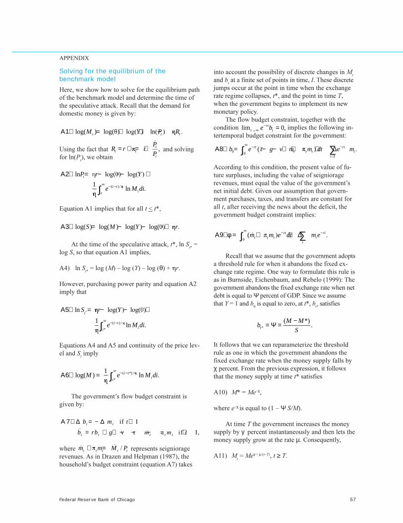
Solving for the equilibrium of thebenchmark model

Here, we show how to solve for the equilibrium pathof the benchmark model and determine the time ofthe speculative attack. Recall that the demand fordomestic money is given by:

log( ) log( � ORJ� � OQ� � �t t tM Y P RΑ1) = + + −

Using the fact that �= + = +&t

t tt

PR r r

P and solving

for ln(Pt), we obtain

( ) /

ln ORJ� � ORJ� �

1ln .

t

i tit

P r Y

e M di∞ − −

Α2) = − − +

∫

Equation A1 implies that for all t < t*,

log( ) log( ) log( ) log( � �S M Y rΑ3) = − − +

At the time of the speculative attack, t*, ln St* =

log S, so that equation A1 implies,

A4) ln St* = log (M) � log (Y) � log (θ) + 0r.

However, purchasing power parity and equation A2imply that

*

( ) /

*


1ln .

t

i tit

S r Y

e M di∞ − −

Α5) = − − +

∫

Equations A4 and A5 and continuity of the price lev-el and S

t imply

( *) /

*

1log( ) ln .i t

itM e M di

∞ − −Α6) = ∫

The government�s flow budget constraint isgiven by:

if I

�LI ,�

Α 7) ∆ = − ∆ ∈

= + + − − − ∉& &t t

t t t t t

b m t

b rb g v P P W

where �t t t t tm m M P+ = && represents seignioragerevenues. As in Drazen and Helpman (1987), thehousehold�s budget constraint (equation A7) takes

into account the possibility of discrete changes in Mt

and bt at a finite set of points in time, I. These discrete

jumps occur at the point in time when the exchangerate regime collapses, t*, and the point in time T,when the government begins to implement its newmonetary policy.

The flow budget constraint, together with thecondition lim 0,−

→∞ =rtt te b implies the following in-

tertemporal budget constraint for the government:

0 0( � �rt ri

t t t ii I

b e g v m m dt e mτ∞ − −

∈

Α8) = − − + + + ∆∑∫ &

According to this condition, the present value of fu-ture surpluses, including the value of seignioragerevenues, must equal the value of the government�snet initial debt. Given our assumption that govern-ment purchases, taxes, and transfers are constant forall t, after receiving the news about the deficit, thegovernment budget constraint implies:

0( � �rt ri

t t t ii

m m e dt m e∞ − −Α9) φ = + + ∆∑∫ &

Recall that we assume that the government adoptsa threshold rule for when it abandons the fixed ex-change rate regime. One way to formulate this rule isas in Burnside, Eichenbaum, and Rebelo (1999): Thegovernment abandons the fixed exchange rate when netdebt is equal to Ψ percent of GDP. Since we assumethat Y = 1 and b

0 is equal to zero, at t*, b

t* satisfies

*

( *).t

M Mb

S

−= Ψ =

It follows that we can reparameterize the thresholdrule as one in which the government abandons thefixed exchange rate when the money supply falls byχ percent. From the previous expression, it followsthat the money supply at time t* satisfies

A10) M* = Me�χ,

where e�χ is equal to (1 � Ψ S/M).

At time T the government increases the moneysupply by γ percent instantaneously and then lets themoney supply grow at the rate µ. Consequently,

A11) Mt = Meγ + µ (t�T), t ≥ T.


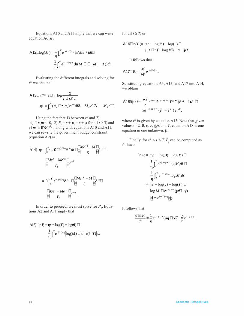
Equations A10 and A11 imply that we can writeequation A6 as,

( *) /

*

( *) /

1log( ) ln( )

1(ln � ��

− − −

∞ − −

Α12) = +

+ + −

∫

∫

Ti t

t

i t

T

M e Me di

e M i T di

Evaluating the different integrals and solving fort* we obtain:

0

* ORJ

( � �rt rt* rTt t t t* T

t T

m m e dt M e M e∞ − − −

Α13) = ++ + η

φ = + + ∆ + ∆∫ &

Using the fact that 1) between t* and T,��t t tm m+ =& 2) R

t = r + π

t = r + µ for all t ≥ T, and

3) ,tRtm Ye−η= θ along with equations A10 and A11,

we can rewrite the government budget constraint(equation A9) as:

� �A14)−χ∞ − + − −

γ −χ−

−φ = + +

−

∫ r rt rt*

T

rT

T

Me MYe e dt e

S

Me Mee

P

� �

.

−− + − −

−−

−= + +

−

r rT rt*

rT

T

Y Me Me e e

r S

Me Mee

P

In order to proceed, we must solve for PT. Equa-

tions A2 and A11 imply that

[ ]( )/

A15) ln ORJ� � ORJ� �

1log( ) � �

∞ − −

= − − +

+ + −∫t

i t

t

P r Y

e M i T di

for all t ≥ T, or

ln( ) ORJ� � ORJ� �

� � ORJ� � �

Α16) = − − ++ + + −

tP r Y

t M T

It follows that

� � .+ +Α17) = rT

MP e

Y

Substituting equations A3, A13, and A17 into A14,we obtain

� �

� �

/ � ��

( ) ,

r rT r rt*

r rT

Ye e Ye e e

r

Ye e e e

− + − − − −

− +µ −γ γ −χ −

Α18) φ = + − +

−

where t* is given by equation A13. Note that givenvalues of φ, θ, 0, r, χ,γ, and T, equation A18 is oneequation in one unknown: µ.

Finally, for t* < t < T, Pt can be computed as

follows:

( ) /

( ) /

( ) /

( ) /


1log

1log

ORJ� � ORJ� �

log ( �

1 �

t

Ti t

it

i tiT

t T

t T

P r Y

e M di

e M di

r Y

M e

e

− −

∞ − −

−

−

= − − +

+

= − − ++ + −

−

∫

∫

It follows that

( ) / � � �ln 1( � �t T t Ttd P

e edt

− −= + +


NOTES

1See Kaminsky and Reinhardt (1999) for an empirical analysis oftwin crises.

2We refer the reader to Burnside, Eichenbaum, and Rebelo (2000a)for a detailed analysis of the modified model.

3Given space constraints, we refer the reader to the papers citedin table 2 for the methodology used to generate these estimates.Basically, the numbers reflect authors� estimates of the aggregatenet worth of protected insolvent institutions.

4Values of the Thai and Korean currencies were obtained from theIMF International Financial Statistics.

5Notice also that there is an overshooting pattern apparent in theexchange rate data, in the sense that each currency appreciatedfrom its value in January 1998 until the end of our sample period,March 2000. Taking this into account, by March 2000, the bahtand won had depreciated by roughly 32 percent and 18 percent oftheir respective pre-crisis values. In this article, we do not formallyaddress possible causes of the overshooting pattern. Burnside,Eichenbaum, and Rebelo (2000a) argue that a version of thebenchmark model in which output first declines and then recoversafter the crises can qualitatively account for the observed over-shooting pattern of exchange rates.

6If banks have open exposure to foreign currency risk, a currencydevaluation will lead to a decline in the real value of banks� assets,reduce their net worth, and result in an increase in bank failures.Burnside, Eichenbaum, and Rebelo (2000b) discuss how govern-ment guarantees to banks� foreign creditors led banks to not hedgethe currency mismatch in their assets and liabilities, leaving themexposed to precisely this kind of currency risk.

7All stock market data were obtained from Bloomberg. The mne-monics for Thailand are SETBANK, SETFIN, and SETCOMM,respectively. For Korea the mnemonics are KOSPBANK,KOSPFIN, and KOSPMAN. These indexes reflect values in localcurrencies.

8Statistics on prices in Thailand were obtained from the �Databank� at the Bank of Thailand website, www.bot.or.th/. Koreanprice data were obtained from the �Statistics� section of the Bankof Korea�s website, www.bok.or.kr/ and from Datastream.

9The data on which this discussion is based are taken from thefollowing sources. Statistics on fiscal indicators for Thailandwere obtained from the Central Bank of Thailand website �Databank� and from IMF (2000b). For Korea, the data were takenfrom IMF (2000a).

10Statistics on GDP in Thailand were obtained from the Bank ofThailand �Data bank� website. Korean GDP data were obtainedfrom the Bank of Korea�s �Statistics� website.

11This last assumption is clearly counterfactual. Burnside,Eichenbaum, and Rebelo (2000a) modify the model to allow fora decline in output after a currency crisis, followed by a recovery.The basic message about the link between prospective deficitsand currency crises remains unaffected by this modification.

12Specifications of money demand like equation 2 are often referredto as �Cagan money demand functions.�

13If there were growth in either the foreign price level or domesticreal income, the government would collect some seigniorage rev-enue in a fixed exchange rate regime. However, this would notaffect our basic argument. The present value of such seignioragerevenues would be pledged to help cover the present value of thedeficit that was anticipated in the initial fixed exchange rate regime.

14Technically, this requirement is given by the conditionlim 0.rt

t te b−→∞ =

15Our basic result would not be affected by a fiscal reform as longas the present value of the change in the primary surplus inducedby the reform was less than φ.

16This result is formally proved in the appendix.

17See, for example, Krugman (1979), Flood and Garber (1984),and Lahiri and Végh (1999).

18Drazen and Helpman (1987), as well as others, have proposed adifferent rule for the government�s behavior: Fix future monetarypolicy and allow the central bank to borrow as much as possibleprovided the present value budget constraint of the government isnot violated. This rule ends up being equivalent to a thresholdrule. See Burnside, Eichenbaum, and Rebelo (1999).

19In our model, the price level at time t is given by:

1 ( ) /ln( ) ln( ) ln( ) ln( ) .∞− − − η= η − θ − + η ∫ i t

t itP r Y e M di

20To see why the speculative attack must occur before time T,suppose to the contrary that the attack actually occurred at time T.Since the government raises the money supply discretely at timeT, inflation and the nominal interest rate would be infinity at T.But then money demand would be zero and the money marketcould not clear.

21It can be shown that whenever equation 8 implies a negativevalue for t*, the exchange rate regime collapses at t = 0. This willhappen for: 1) sufficiently high interest elasticities of money de-mand; 2) low values of χ, or 3) large values of γ and µ requiredto finance the prospective deficit. In this case the exchange ratewill jump at time zero. This does not contradict our argument thatthe exchange rate path must be continuous. This is because thediscontinuity in the exchange rate at time zero coincides with thearrival of the unanticipated news about prospective deficits.

22For example, in the model, the inflation rate during the yearfrom October 1997 to October 1998 is 11.25 percent. The inflationrate in the year after is roughly 4 percent. The correspondingrates of CPI inflation in the Korean data are roughly 7 percentand 1 percent, respectively.

23Burnside, Eichenbaum, and Rebelo (2000a) also discuss the im-plications of relaxing the assumption that output is constant afterthe speculative attack.

24For example, steady-state inflation in the modified model dropsby a factor of three relative to its value in the benchmark model.

25Burnside, Eichenbaum, and Rebelo (2000c) analyze a model inwhich government guarantees to banks� foreign creditors implythat a currency crisis will almost surely occur. But the time atwhich it occurs is stochastic.


NOTES

Burnside, Craig, Martin Eichenbaum, and SergioRebelo, 2000a, �How do governments pay for twincrises?,� Northwestern University, manuscript.

, 2000b, �Hedging and financial fragilityin fixed exchange rate regimes,� European EconomicReview, forthcoming.

, 2000c, �On the fundamentals of selffulfilling currency crises,� Northwestern University,manuscript.

, 1999, �Prospective deficits and theAsian currency crises,� Northwestern University,mimeo.

Burstein, Ariel, Joao Neves, and Sergio Rebelo,2000, �Distribution costs and real exchange ratedynamics during exchange-rate-based stabilizations,�Northwestern University, mimeo.

Caprio, Jr., G., and D. Klingebiel, 1996, �Bank in-solvencies: Cross country experience,� World Bank,working paper, No. 1620.

Corsetti, Giancarlo, Paolo Pesenti, and NourielRoubini, 1999, �What caused the Asian currencyand financial crisis?,� Japan and the World Economy,Vol. 11, pp. 305�373.

Drazen, Allan, and Elhanan Helpman, 1987,�Stabilization with exchange rate management,� Quar-terly Journal of Economics, Vol. 102, pp. 835�855.

Dziobek, C., and C. Pazarbasioglu, 1997, �Lessonsfrom systematic bank restructuring: A survey of 24countries,� International Monetary Fund, workingpaper, No. 97/161.

Easterly, William, Paolo Mauro, Klaus Schmidt-Hebbel, 1995, �Money demand and seigniorage-maximizing inflation,� Journal of Money, Credit,and Banking, Vol. 27, pp. 583�603.

Flood, Robert, and Peter Garber, 1984, �Collapsingexchange rate regimes: Some linear examples,� Jour-nal of International Economics, Vol. 17, pp. 1�13.

Frydl, Edward, 1999, �The length and cost of bank-ing crises,� International Monetary Fund, workingpaper, No. WP/99/30.

International Monetary Fund, 2000a, �Republicof Korea: Statistical appendix,� staff country report,No. 00/10, February.

, 2000b, �Thailand: Statistical appendix,�staff country report, No. 00/20, February.

J. P. Morgan, 1998, �Asian financial markets, thirdquarter 1998,� report, July 17.

Kaminsky, Graciela, and Carmen Reinhart, 1999,�The twin crises: The causes of banking and balance-of-payments problems,� American Economic Review,Vol. 89, pp. 473�500.

Krugman, Paul, 1979, �A model of balance of pay-ments crises,� Journal of Money, Credit, and Banking,Vol. 11, pp. 311�325.

Lahiri, Amartya, and Carlos Végh, 1999, �Delayingthe inevitable: Optimal interest rate policy and BOPcrises,� University of California, Los Angeles, mimeo.

Lindgren, C-J., G. Garcia, and M. I. Saal, 1996,Bank Soundness and Macroeconomic Policy, Wash-ington: International Monetary Fund.

Polackova, H., 1999, �Contingent government liabili-ties: A hidden fiscal risk,� Finance and Development,A Quarterly Magazine of the IMF, Vol. 36, No. 1.

Sargent, Thomas, and Neil Wallace, 1981, �Someunpleasant monetarist arithmetic,� Quarterly Review,Federal Reserve Bank of Minneapolis, Vol. 5, pp. 1�17.

Documents

Understanding the Korean and Thai currency crises Reserve Bank of Chicago 45 Understanding the Korean and Thai currency crises Craig Burnside, Martin Eichenbaum, and Sergio Rebelo