Understanding the hydrological impacts of climate change

Understanding the Hydrological Impacts of Climate Change in the Tana River Basin, Kenya

IWMI Working Paper

178Aditya Sood, Lal Muthuwatta, Nishchitha Sandeepana Silvaand Matthew McCartney

Working Papers

The publications in this series record the work and thinking of IWMI researchers, and knowledge that the Institute’s scientific management feels is worthy of documenting. This series will ensure that scientific data and other information gathered or prepared as a part of the research work of the Institute are recorded and referenced. Working Papers could include project reports, case studies, conference or workshop proceedings, discussion papers or reports on progress of research, country-specific research reports, monographs, etc. Working Papers may be copublished, by IWMI and partner organizations.

Although most of the reports are published by IWMI staff and their collaborators, we welcome contributions from others. Each report is reviewed internally by IWMI staff. The reports are published and distributed both in hard copy and electronically (www.iwmi.org) and where possible all data and analyses will be available as separate downloadable files. Reports may be copied freely and cited with due acknowledgment.

About IWMI

IWMI’s mission is to provide evidence-based solutions to sustainably manage water and land resources for food security, people’s livelihoods and the environment. IWMI works in partnership with governments, civil society and the private sector to develop scalable agricultural water management solutions that have a tangible impact on poverty reduction, food security and ecosystem health.

IWMI Working Paper 178

Understanding the Hydrological Impacts of Climate Change in the Tana River Basin, Kenya

Aditya Sood, Lal Muthuwatta, Nishchitha Sandeepana Silvaand Matthew McCartney

International Water Management Institute

A free copy of this publication can be downloaded atwww.iwmi.org/Publications/Working_Papers/index.aspx

The authors: Aditya Sood is Lead Freshwater Scientist at The Nature Conservancy, New Delhi, India; He was Senior Researcher – Integrated Hydrological Modelling at the International Water Management Institute (IWMI), Colombo, Sri Lanka, at the time this research study was conducted; Lal Muthuwatta is Regional Researcher – Hydrological Modeling & Remote Sensing at IWMI, Colombo, Sri Lanka; Nishchitha Sandeepana Silva was an intern at IWMI, Colombo, Sri Lanka, and is currently pursuing a Master of Science in Marine Science and Technology at the University of Massachusetts Dartmouth, School for Marine Science and Technology, Massachusetts, USA; and Matthew McCartney is Research Group Leader - Water Futures, Growth and Natural Capital at IWMI, Vientiane, Lao People’s Democratic Republic.

Sood, A.; Muthuwatta, L.; Silva, N. S.; McCartney, M. 2017. Understanding the hydrological impacts of climate change in the Tana River Basin, Kenya. Colombo, Sri Lanka: International Water Management Institute (IWMI). 40p. (IWMI Working Paper 178). doi: 10.5337/2017.220

/ climate change / rain / evapotranspiration / flooding / river basin / hydrology / discharges / water yield / groundwater recharge / natural resources / infrastructure / land use / ecosystem services / soil water / simulation models / Kenya /

ISSN 2012-5763e-ISSN 2478-1134 ISBN 978-92-9090-860-9

Copyright 2017, by IWMI. All rights reserved. IWMI encourages the use of its material provided that the organization is acknowledged and kept informed in all such instances.

Please direct inquiries and comments to: [email protected]

Acknowledgements

Project

This work was undertaken as part of the Water Infrastructure Solutions from Ecosystem Services Underpinning Climate Resilient Policies and Programmes (WISE-UP to Climate) project. This project aims to demonstrate how natural infrastructure as a ‘nature-based solution’ contributes to climate change adaptation and sustainable development. The project has developed knowledge and options on the use of portfolios of built water infrastructure (e.g., dams,

levees, irrigation channels) and natural infrastructure (e.g., wetlands, floodplains, watersheds) for poverty reduction, water-energy-food security, biodiversity conservation, and climate resilience. The project is working in the Volta River Basin (Ghana, principally, and also Burkina Faso) as well as the Tana River Basin in Kenya.

The project is led by the International Union for Conservation of Nature (IUCN) and involves the Council for Scientific and Industrial Research - Water Research Institute (CSIR-WRI); African Collaboration Centre for Earth System Science (ACCESS), University of Nairobi; International Water Management Institute (IWMI); Overseas Development Institute (ODI); University of Manchester; and the Basque Centre for Climate Change (BC3). The project is part of the International Climate Initiative. Bundesministerium für Umwelt, Naturschutz, Bau und Reaktorsicherheit (BMUB) (Federal Ministry for the Environment, Nature Conservation, Building and Nuclear Safety), Germany, support this initiative on the basis of a decision adopted by the German Bundestag.

For further details about the project, visit: www.waterandnature.org or www.iucn.org/water_wiseup

Donors

Bundesministerium für Umwelt, Naturschutz, Bau und Reaktorsicherheit (BMUB) (Federal Ministry for the Environment, Nature Conservation, Building and Nuclear Safety), Germany.

This research was carried out as part of the CGIAR Research Program on Water, Land and Ecosystems (WLE) and supported by CGIAR Fund Donors (http://www.cgiar.org/about-us/ourfunders/).

v

Contents

Acronyms and Abbreviations ..................................................................................................... vi

Summary ............................................................................................................................ vii

Introduction .............................................................................................................................. 1

Study Area .............................................................................................................................. 2

Rainfall .............................................................................................................................. 3

Evapotranspiration .............................................................................................................. 5

Methodology and Data ................................................................................................................ 6

SWAT Setup ........................................................................................................................ 8

Calibration and Validation ................................................................................................ 12

Results and Discussion .............................................................................................................. 15

Climate Change ................................................................................................................. 16

Rainfall ..................................................................................................................... 16

Basin Flow ................................................................................................................ 19

Impact on Floods ...................................................................................................... 23

Type 1 Ecosystem Services ...................................................................................... 24

Conclusion ............................................................................................................................ 27

References ............................................................................................................................ 28

Annex 1. Summary of Individual Model Results. .................................................................... 29

vi

Acronyms and Abbreviations

AR Assessment ReportCC Climate ChangeCFSR Climate Forecast System ReanalysisCORDEX Coordinated Regional Climate Downscaling ExperimentCUP Calibration and Uncertainty ProgramDEM Digital Elevation ModelES Ecosystem ServiceFAO Food and Agriculture Organization of the United NationsGCM Global Circulation ModelGHG Greenhouse GasGLUE Generalized Likelihood Uncertainty EstimationGoK Government of Kenya HRU Hydrological Response UnitIPCC Intergovernmental Panel on Climate ChangeKMD Kenya Meteorological DepartmentMCMC Markov Chain Monte CarloNCEP National Centers for Environmental PredictionNMD National Meteorological DepartmentNSE Nash-Sutcliffe EfficiencyParaSol Parameter SolutionPET Potential EvapotranspirationPPU Percentage Prediction UncertaintyPSO Particle Swarm OptimizationRCM Regional Circulation ModelRCP Representative Concentration PathwaySRTM Shuttle Radar Topography MissionSUFI Sequential Uncertainty FittingSWAT Soil and Water Assessment Tool TCM Tana Climate ModelWRMA Water Resources Management Agency

vii

Summary

Seven Regional Circulation Models (RCMs), simulating two Representative Concentration Pathways (i.e., RCPs 4.5 and 8.5), were used as input to the Soil and Water Assessment Tool (SWAT) model to determine the possible impacts of climate change on the hydrology of the Tana River Basin in Kenya. Four hydrological characteristics – water yield, groundwater recharge, baseflow and flow regulation - were determined and mapped throughout the basin for three 30-year time periods: 2020-2049, 2040-2069 and 2070-2099. Results show a spatial heterogeneity with clear differences between the upper, middle and lower basins. Simulation of both RCPs indicate an increase in mean annual rainfall for all three time periods, with an earlier onset of rainfall in some model simulations. The majority of models indicate an increase in extreme climate events under both RCPs. The response of the basin to the increase in rainfall is not linear, and the simulated increases in water yield, groundwater recharge and baseflow are much higher (in percentage terms) than the changes in rainfall. The impacts of climate change will be superimposed onto a basin with complex land use, built infrastructure and an intricate sociopolitical history. The results have important implications for the management of both built and natural infrastructure in the basin.

1

IntroductIon

As part of the Water Infrastructure Solutions from Ecosystem Services underpinning Climate Resilient Policies and Programmes (WISE-UP to Climate) project, two types of ecosystem services (ESs) have been recognized in relation to the interactions between natural infrastructure (e.g., forests, wetlands, floodplains) and built water infrastructure (e.g., dams, levees, irrigation channels): (i) Type 1 ESs are defined as those that affect the technical performance of built water infrastructure. These are typically characteristics of the hydrological regime that are affected by natural processes and influence the ability of the built infrastructure to deliver intended benefits; and (ii) Type 2 ESs are defined as those that are affected by the presence of built water infrastructure. These are typically services which are modified by the physical presence of the built water infrastructure or by changes in water/sediment/nutrient fluxes that are altered as a consequence of the way the infrastructure is designed and operated (McCartney et al. Forthcoming).

In the component of the study described here, a hydrological model, the Soil and Water Assessment Tool (SWAT), was used to simulate type 1 ESs in the Tana River Basin, Kenya. The model was used to quantify and map hydrological processes designated as type 1 ESs because they influence the technical performance of the five major dams in the basin. The model was configured and calibrated for the current situation and then used to determine the possible impacts of climate change (CC) on type 1 ESs.

Many studies have been conducted to simulate the impacts of CC in the basin. Nakaegawa et al. (2012) produced hydrological cycle projections under CC. Their analysis projected significant increases in: (i) annual mean precipitation (15% across the entire basin); (ii) evaporation (though with significant geographical contrasts between the eastern and western parts of the basin); (iii) total runoff and river discharge (more than 50%); and (iv) soil water storage.

Wamuongo et al. (2014) investigated climatic vulnerability, risks and impacts on food and livestock production systems in three Tana Delta project sites: Kisuliani, Matoba and Kipini. They conducted an analysis of long-term climatic data in the Tana River Basin and found a general decline in rainfall for the period 1961-1990, with a trend toward predominantly increased precipitation by 2030, 2050 and 2080 compared to current mean rainfall. The spatial plots of rainfall indicate seasonal differences, but with a high percentage increase over some Tana counties during March to May under the Representative Concentration Pathway (RCP) 4.5. During the October-December season, all sites showed increased rainfall, but of a lower intensity compared to the March-May season.

Leauthaud et al. (2013) noted that, over the past 50 years, five major reservoirs have been built in the basin, resulting in a 20% decrease in downstream peak flows in May. Droogers et al. (2009) used projections from nine Global Circulation Models (GCMs) for their study on the impacts of CC on hydropower generation in the Tana River Basin. These projections produced mixed results, but, on average (i.e., averaging projections for all nine GCMs for every month), the percentage increase in monthly rainfall ranged from less than 5% (August and November) to 35% (September). Although rainfall increased, evapotranspiration also increased, and in conjunction with higher water demand, resulted in slightly lower inflow into the reservoirs. For instance, average water demand under the current situation is 684 million cubic meters per year (Mm3y-1); this will increase to between 781 and 873 Mm3 y-1 under different CC scenarios. Further analysis showed that the average hydropower generation will reduce from 2,253 gigawatt hours per year (GWhy-1) to levels between 1,763 and 2,144 GWhy-1.

2

For this study, the latest CC projections were used. The results from seven Regional Circulation Models (RCMs) were used to provide input to the SWAT model. The simulation results were used to assess the impacts on hydrological processes/water fluxes that can be considered as type 1 ESs (i.e., water yield, groundwater recharge, baseflow and flow regulation).

Study AreA

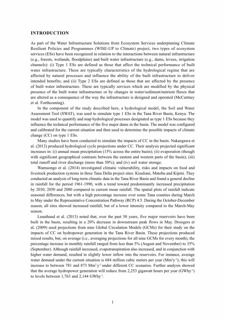
The Tana River (Figure 1) is the longest river in Kenya, originating in the Aberdare Mountains, west of Nyeri, and flowing for over 1,000 km to meet the Indian Ocean in the Ungwana Bay-Kipini area. The river drains a catchment area of 95,000 km2. The Tana River Basin covers 21% of the country’s total landmass and is home to 18% of the country’s population. It contributes over 50% of Kenya’s river discharge to the Western Indian Ocean. Ecosystems in the Tana River Basin, including forests, arid and semiarid lands, mountain vegetation, freshwater and wetlands, marine and coastal areas, and agroecosystems, provide a range of ecosystem services that are vital for human well-being. For example, the basin supplies 80% of the drinking water for Kenya’s capital, Nairobi. The Tana River is also the country’s primary source of hydroelectric power (i.e., 70% of Kenya’s hydroelectricity and 38% of total electricity supply). Fisheries and agriculture in the basin provide a major source of food and employment for the estimated 7 million residents that live in the greater basin area and many more in other parts of the country. One of the basin’s important ecosystems is the Tana Delta at the coast. This biodiversity hot spot is home to several endangered species and was designated as a Ramsar site in 2012.

In Kenya, there is recognition at the highest levels of government that climate change is a key priority and that adaptation and development goals need to complement each other (GoK 2012). However, a recent political economy analysis of decision making related to the development of water infrastructure in Kenya found that water governance in the country is highly fragmented with many players, overlapping mandates and institutional rivalries (Oates and Marani 2017). CC and the uncertainty associated with it further complicate the planning and management of the country’s water resources, including those of the Tana River basin.

For this study, the basin was divided into three zones based on the average altitude of each sub-basin, as delineated by SWAT: (i) Upper zone – average altitude greater than 2,400 m; (ii) Middle zone – average altitude between 600 m and 2,400 m; and (iii) Lower zone – average altitude below 600 m. ArcGIS was used to calculate the average altitude of each sub-basin. The areas in the Upper, Middle and Lower zones are 1,514 km2, 29,890 km2 and 52,568 km2, respectively1 (Figure 1).

1 Note: The sum of these areas is 83,972 km2. This is because the area simulated within the SWAT model was to Garsen (the most downstream flow gauging station) rather than the outlet to the sea.

3

FIGURE 1. Tana River Basin showing the three zones based on the average altitude of each sub-basin.

rainfall

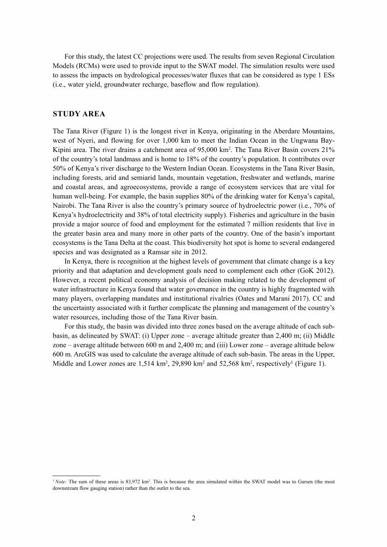
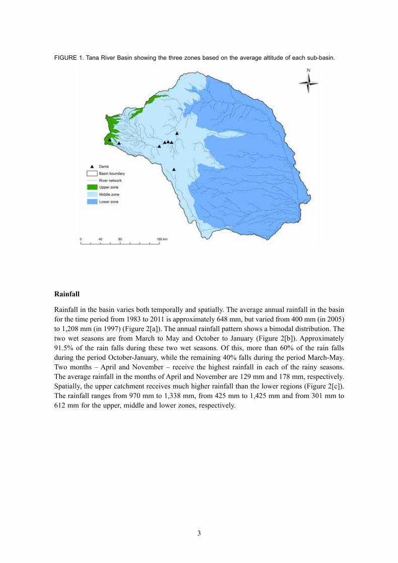
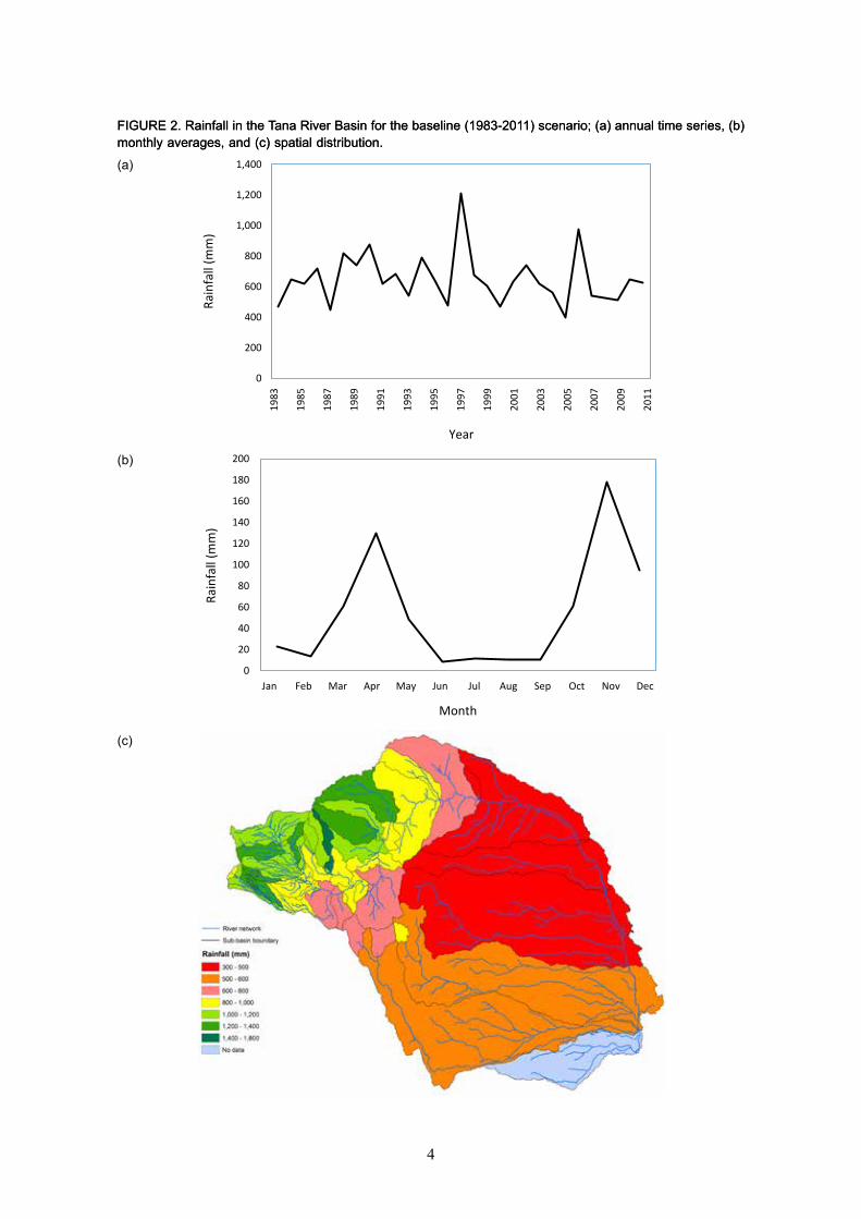
Rainfall in the basin varies both temporally and spatially. The average annual rainfall in the basin for the time period from 1983 to 2011 is approximately 648 mm, but varied from 400 mm (in 2005) to 1,208 mm (in 1997) (Figure 2[a]). The annual rainfall pattern shows a bimodal distribution. The two wet seasons are from March to May and October to January (Figure 2[b]). Approximately 91.5% of the rain falls during these two wet seasons. Of this, more than 60% of the rain falls during the period October-January, while the remaining 40% falls during the period March-May. Two months – April and November – receive the highest rainfall in each of the rainy seasons. The average rainfall in the months of April and November are 129 mm and 178 mm, respectively. Spatially, the upper catchment receives much higher rainfall than the lower regions (Figure 2[c]). The rainfall ranges from 970 mm to 1,338 mm, from 425 mm to 1,425 mm and from 301 mm to 612 mm for the upper, middle and lower zones, respectively.

4

FIGURE 2. Rainfall in the Tana River Basin for the baseline (1983-2011) scenario; (a) annual time series, (b) monthly averages, and (c) spatial distribution.FIGURE 2. Rainfall in the Tana River Basin for the baseline (1983-2011) scenario; (a) annual time series, (b) monthly averages, and (c) spatial distribution.

0

200

400

600

800

1,000

1,200

1,400

1983

1985

1987

1989

1991

1993

1995

1997

1999

2001

2003

2005

2007

2009

2011

Rain

fall

(mm

)

Year

(a)

(b)

(c)

Month

0

20

40

60

80

100

120

140

160

180

200

Jan Feb Mar Apr May Jun Jul Aug Sep Oct Nov Dec

Rain

fall

(mm

)

5

evapotranspiration

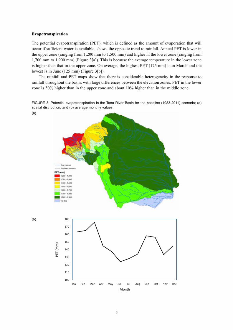
The potential evapotranspiration (PET), which is defined as the amount of evaporation that will occur if sufficient water is available, shows the opposite trend to rainfall. Annual PET is lower in the upper zone (ranging from 1,200 mm to 1,500 mm) and higher in the lower zone (ranging from 1,700 mm to 1,900 mm) (Figure 3[a]). This is because the average temperature in the lower zone is higher than that in the upper zone. On average, the highest PET (175 mm) is in March and the lowest is in June (125 mm) (Figure 3[b]).

The rainfall and PET maps show that there is considerable heterogeneity in the response to rainfall throughout the basin, with large differences between the elevation zones. PET in the lower zone is 50% higher than in the upper zone and about 10% higher than in the middle zone.

FIGURE 3. Potential evapotranspiration in the Tana River Basin for the baseline (1983-2011) scenario; (a) spatial distribution, and (b) average monthly values.(a)

(b)

100

110

120

130

140

150

160

170

180


PET

(mm

)

Month

6

Methodology And dAtA

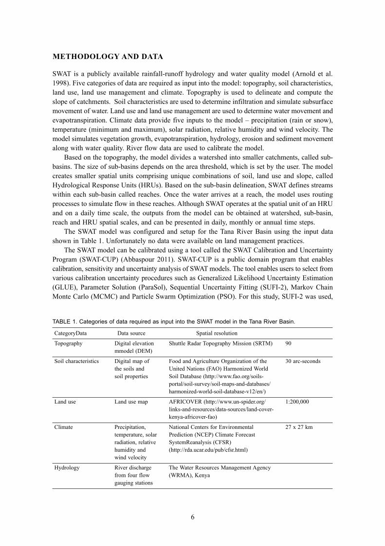
SWAT is a publicly available rainfall-runoff hydrology and water quality model (Arnold et al. 1998). Five categories of data are required as input into the model: topography, soil characteristics, land use, land use management and climate. Topography is used to delineate and compute the slope of catchments. Soil characteristics are used to determine infiltration and simulate subsurface movement of water. Land use and land use management are used to determine water movement and evapotranspiration. Climate data provide five inputs to the model – precipitation (rain or snow), temperature (minimum and maximum), solar radiation, relative humidity and wind velocity. The model simulates vegetation growth, evapotranspiration, hydrology, erosion and sediment movement along with water quality. River flow data are used to calibrate the model.

Based on the topography, the model divides a watershed into smaller catchments, called sub-basins. The size of sub-basins depends on the area threshold, which is set by the user. The model creates smaller spatial units comprising unique combinations of soil, land use and slope, called Hydrological Response Units (HRUs). Based on the sub-basin delineation, SWAT defines streams within each sub-basin called reaches. Once the water arrives at a reach, the model uses routing processes to simulate flow in these reaches. Although SWAT operates at the spatial unit of an HRU and on a daily time scale, the outputs from the model can be obtained at watershed, sub-basin, reach and HRU spatial scales, and can be presented in daily, monthly or annual time steps.

The SWAT model was configured and setup for the Tana River Basin using the input data shown in Table 1. Unfortunately no data were available on land management practices.

The SWAT model can be calibrated using a tool called the SWAT Calibration and Uncertainty Program (SWAT-CUP) (Abbaspour 2011). SWAT-CUP is a public domain program that enables calibration, sensitivity and uncertainty analysis of SWAT models. The tool enables users to select from various calibration uncertainty procedures such as Generalized Likelihood Uncertainty Estimation (GLUE), Parameter Solution (ParaSol), Sequential Uncertainty Fitting (SUFI-2), Markov Chain Monte Carlo (MCMC) and Particle Swarm Optimization (PSO). For this study, SUFI-2 was used,

TABLE 1. Categories of data required as input into the SWAT model in the Tana River Basin.

Category Data Data source Spatial resolution

Topography Digital elevation Shuttle Radar Topography Mission (SRTM) 90 mmodel (DEM)

Soil characteristics Digital map of Food and Agriculture Organization of the 30 arc-seconds the soils and United Nations (FAO) Harmonized World soil properties Soil Database (http://www.fao.org/soils- portal/soil-survey/soil-maps-and-databases/ harmonized-world-soil-database-v12/en/)

Land use Land use map AFRICOVER (http://www.un-spider.org/ 1:200,000 links-and-resources/data-sources/land-cover- kenya-africover-fao)

Climate Precipitation, National Centers for Environmental 27 x 27 km temperature, solar Prediction (NCEP) Climate Forecast radiation, relative SystemReanalysis (CFSR) humidity and (http://rda.ucar.edu/pub/cfsr.html) wind velocity

Hydrology River discharge The Water Resources Management Agency from four flow (WRMA), Kenya gauging stations

7

as it is the most commonly used procedure for SWAT model calibration and has been successfully used in a number of studies around the world (e.g., Abbaspour et al. 2007; Sood et al. 2013). Two parameters are used to quantify uncertainty in the model: P-factor and R-factor. The P-factor indicates the percentage of the observed data that falls within 95% of prediction uncertainty (95PPU), and the R-factor is the average thickness of the 95PPU band divided by the standard deviation of the observed data. Two performance indicators – Nash-Sutcliffe Efficiency (NSE) (Nash and Sutcliffe 1970) and Coefficient of Determination (R2) – were used to evaluate model simulations.

Once the SWAT model was calibrated, it was run from 1983 to 2011 to develop a current (or baseline) scenario. Hydrological characteristics that are critical to the functioning and hence performance of dams (i.e., built infrastructure) relate to the quantity and temporal distribution of flow into reservoirs. Both factors are influenced by natural infrastructure – land cover, land management and land-use practices. Effectively, the ‘performance’ of natural infrastructure influences the performance of built infrastructure. Hydrological parameters, which can be used to categorize the services provided by natural infrastructure, are water yield, groundwater recharge, baseflow and flow regulation (Table 2).

Multiple CC scenarios were run using the SWAT model to determine the impact of CC on Type 1 ESs of the Tana River Basin. CC scenarios are developed using GCMs, but these have coarse spatial resolution and fail to consider local conditions. Thus, for regional studies, GCMs may not provide realistic CC outcomes. This is overcome by downscaling and/or bias correction based on regional information. Downscaling can be dynamic, wherein a nested climate model, Regional Climate Model (RCM), is used, or it can be statistical, whereby empirical relationships between simulated and observed data are used.

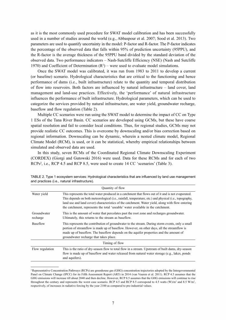
In this study, seven RCMs of the Coordinated Regional Climate Downscaling Experiment (CORDEX) (Giorgi and Gutowski 2016) were used. Data for these RCMs and for each of two RCPs2, i.e., RCP 4.5 and RCP 8.5, were used to create 14 CC ‘scenarios’ (Table 3).

TABLE 2. Type 1 ecosystem services: Hydrological characteristics that are influenced by land use management and practices (i.e., natural infrastructure).

Quantity of flow

Water yield This represents the total water produced in a catchment that flows out of it and is not evaporated. This depends on both meteorological (i.e., rainfall, temperature, etc.) and physical (i.e., topography, land use and land cover) characteristics of the catchment. Water yield, along with flow entering the catchment, represents the total ‘useable’ water available in the catchment.

Groundwater This is the amount of water that percolates past the root zone and recharges groundwater. recharge Ultimately, this returns to the stream as baseflow.

Baseflow This represents the contribution of groundwater to the stream. During storm events, only a small portion of streamflow is made up of baseflow. However, on other days, all the streamflow is made up of baseflow. The baseflow depends on the aquifer properties and the amount of groundwater recharge that takes place.

Timing of flow

Flow regulation This is the ratio of dry-season flow to total flow in a stream. Upstream of built dams, dry-season flow is made up of baseflow and water released from natural water storage (e.g., lakes, ponds and aquifers).

2 Representative Concentration Pathways (RCPs) are greenhouse gas (GHG) concentration trajectories adopted by the Intergovernmental Panel on Climate Change (IPCC) for its Fifth Assessment Report (AR5) in 2014 (van Vuuren et al. 2011). RCP 4.5 assumes that the GHG emissions will increase till about 2040 and then decline. However, RCP 8.5 assumes that the GHG emissions will continue to rise throughout the century and represents the worst case scenario. RCP 4.5 and RCP 8.5 correspond to 4.5 watts (W)/m2 and 8.5 W/m2, respectively, of increases in radiative forcing by the year 2100 as compared to pre-industrial values.

8

The model was run for the period 2011-2099, and data were analyzed for the three periods 2020-2049, 2040-2069 and 2070-2099.

TABLE 3. Climate change scenarios used in this study for the Tana River Basin.

Institution Driving GCM RCM RCP Scenario name+

CCCma-CanESM2 CCCma-CanRCM4 RCP 4.5 TCM1-45

CCCma-CanESM2 CCCma-CanRCM4 RCP 8.5 TCM1-85

CNRM-CERFACS-CNRM-CM5 CLMcom-CCLM4-8-17 RCP 4.5 TCM2-45

CNRM-CERFACS-CNRM-CM5 CLMcom-CCLM4-8-17 RCP 8.5 TCM2-85

ICHEC-EC-EARTH CLMcom-CCLM4-8-17 RCP 4.5 TCM3-45

ICHEC-EC-EARTH CLMcom-CCLM4-8-17 RCP 8.5 TCM3-85

MOHC-HadGEM2-ES CLMcom-CCLM4-8-17 RCP 4.5 TCM4-45

MOHC-HadGEM2-ES CLMcom-CCLM4-8-17 RCP 8.5 TCM4-85

MPI-M-MPI-ESM-LR CLMcom-CCLM4-8-17 RCP 4.5 TCM5-45

MPI-M-MPI-ESM-LR CLMcom-CCLM4-8-17 RCP 8.5 TCM5-85

ICHEC-EC-EARTH KNMI-RACMO22T RCP 4.5 TCM6-45

ICHEC-EC-EARTH KNMI-RACMO22T RCP 8.5 TCM6-85

IPSL-IPSL-CM5A-MR SMHI-RCA4 RCP 4.5 TCM7-45

IPSL-IPSL-CM5A-MR SMHI-RCA4 RCP 8.5 TCM7-85

Canadian Centre for Climate Modelling and Analysis (CCCma)

Swedish Meteorological and Hydrological Institute

Royal Netherlands Meteorological Institute

Climate Limited- area Modelling Community

Note: + TCM - Tana Climate Model.

SWAt Setup

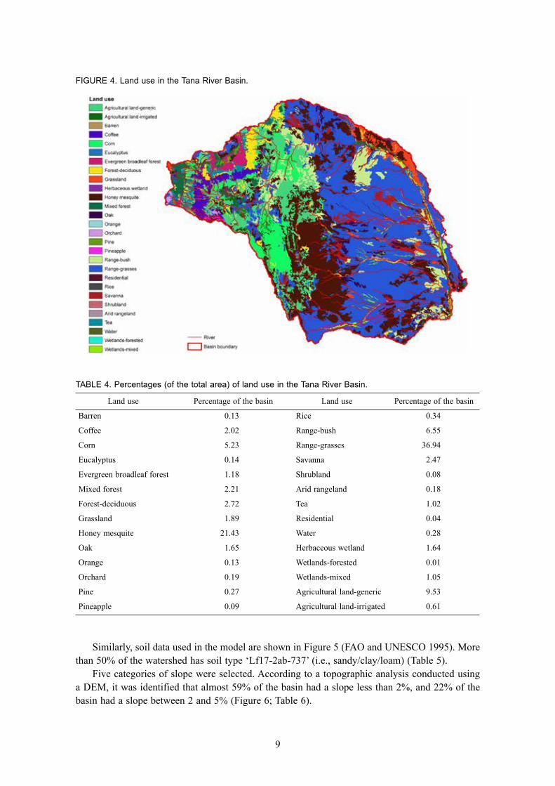
The model was setup using the inputs as described above. An area threshold of 20.0 km2 was used to define the sub-basin and HRU delineation process. This led to the creation of 368 sub-basins.Land use, as shown in Figure 4, was used (http://www.waterbase.org/download_data.html). The two largest land covers in the watershed are grass rangeland and honey mesquite (a species of small to medium-sized thorny shrub or tree in the legume family), which cover about 37% and 21% of the watershed, respectively. Forest cover (evergreen broadleaf forest, mixed forest and forest-deciduous) is about 6% and agriculture is about 10.5% of the total catchment area (Table 4).

9

FIGURE 4. Land use in the Tana River Basin.

TABLE 4. Percentages (of the total area) of land use in the Tana River Basin.

Land use Percentage of the basin Land use Percentage of the basin

Barren 0.13 Rice 0.34

Coffee 2.02 Range-bush 6.55

Corn 5.23 Range-grasses 36.94

Eucalyptus 0.14 Savanna 2.47

Evergreen broadleaf forest 1.18 Shrubland 0.08

Mixed forest 2.21 Arid rangeland 0.18

Forest-deciduous 2.72 Tea 1.02

Grassland 1.89 Residential 0.04

Honey mesquite 21.43 Water 0.28

Oak 1.65 Herbaceous wetland 1.64

Orange 0.13 Wetlands-forested 0.01

Orchard 0.19 Wetlands-mixed 1.05

Pine 0.27 Agricultural land-generic 9.53

Pineapple 0.09 Agricultural land-irrigated 0.61

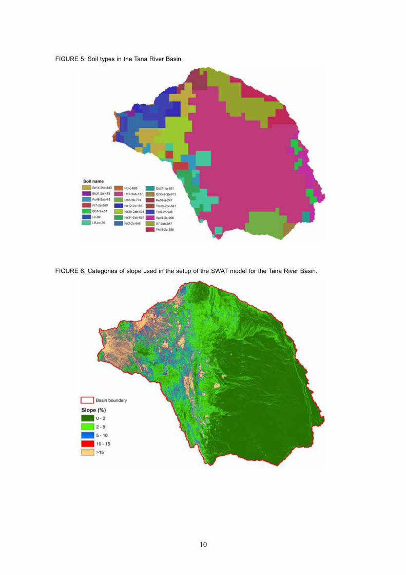
Similarly, soil data used in the model are shown in Figure 5 (FAO and UNESCO 1995). More than 50% of the watershed has soil type ‘Lf17-2ab-737’ (i.e., sandy/clay/loam) (Table 5).

Five categories of slope were selected. According to a topographic analysis conducted using a DEM, it was identified that almost 59% of the basin had a slope less than 2%, and 22% of the basin had a slope between 2 and 5% (Figure 6; Table 6).

10

FIGURE 5. Soil types in the Tana River Basin.

FIGURE 6. Categories of slope used in the setup of the SWAT model for the Tana River Basin.

11

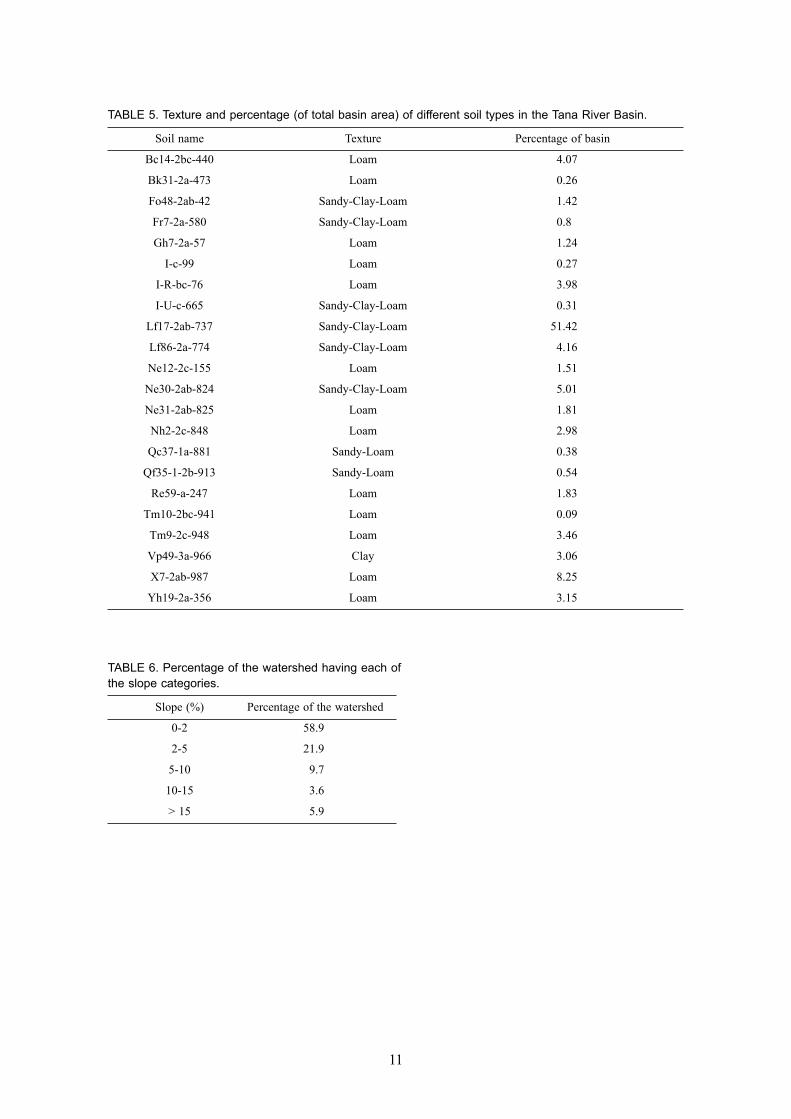
TABLE 5. Texture and percentage (of total basin area) of different soil types in the Tana River Basin.

Soil name Texture Percentage of basin

Bc14-2bc-440 Loam 4.07

Bk31-2a-473 Loam 0.26

Fo48-2ab-42 Sandy-Clay-Loam 1.42

Fr7-2a-580 Sandy-Clay-Loam 0.8

Gh7-2a-57 Loam 1.24

I-c-99 Loam 0.27

I-R-bc-76 Loam 3.98

I-U-c-665 Sandy-Clay-Loam 0.31

Lf17-2ab-737 Sandy-Clay-Loam 51.42

Lf86-2a-774 Sandy-Clay-Loam 4.16

Ne12-2c-155 Loam 1.51

Ne30-2ab-824 Sandy-Clay-Loam 5.01

Ne31-2ab-825 Loam 1.81

Nh2-2c-848 Loam 2.98

Qc37-1a-881 Sandy-Loam 0.38

Qf35-1-2b-913 Sandy-Loam 0.54

Re59-a-247 Loam 1.83

Tm10-2bc-941 Loam 0.09

Tm9-2c-948 Loam 3.46

Vp49-3a-966 Clay 3.06

X7-2ab-987 Loam 8.25

Yh19-2a-356 Loam 3.15

TABLE 6. Percentage of the watershed having each of the slope categories.

Slope (%) Percentage of the watershed

0-2 58.9

2-5 21.9

5-10 9.7

10-15 3.6

> 15 5.9

12

Thresholds of 20%, 20% and 30% were used for land use, soil and slope, respectively, to create HRUs. The selection of thresholds is subjective and depends on the level of detail required and the computational limitations. Lower values of threshold lead to a higher number of HRUs, but increase the model processing time. The thresholds selected in this study led to the creation of 1,047 HRUs.

calibration and Validation

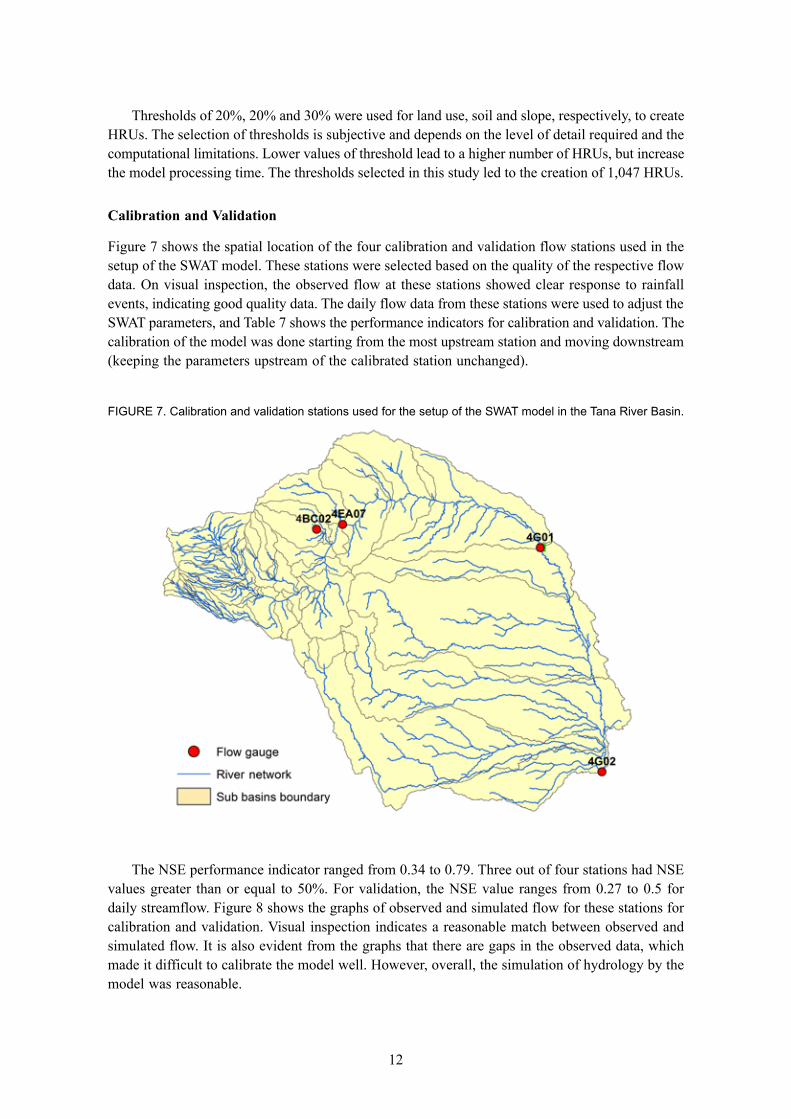
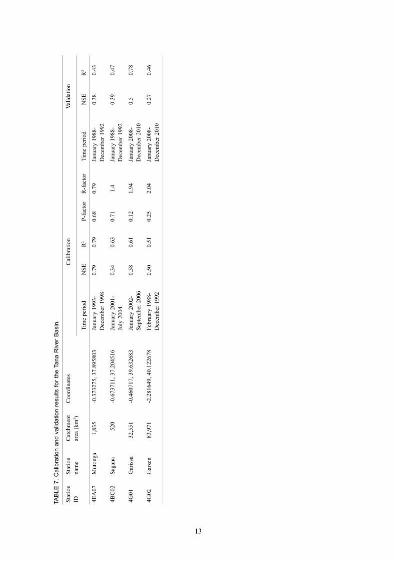
Figure 7 shows the spatial location of the four calibration and validation flow stations used in the setup of the SWAT model. These stations were selected based on the quality of the respective flow data. On visual inspection, the observed flow at these stations showed clear response to rainfall events, indicating good quality data. The daily flow data from these stations were used to adjust the SWAT parameters, and Table 7 shows the performance indicators for calibration and validation. The calibration of the model was done starting from the most upstream station and moving downstream (keeping the parameters upstream of the calibrated station unchanged).

FIGURE 7. Calibration and validation stations used for the setup of the SWAT model in the Tana River Basin.

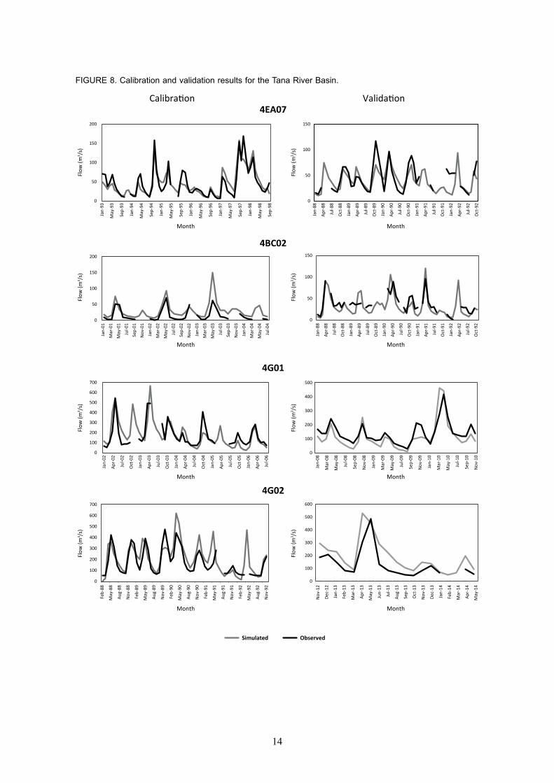
The NSE performance indicator ranged from 0.34 to 0.79. Three out of four stations had NSE values greater than or equal to 50%. For validation, the NSE value ranges from 0.27 to 0.5 for daily streamflow. Figure 8 shows the graphs of observed and simulated flow for these stations for calibration and validation. Visual inspection indicates a reasonable match between observed and simulated flow. It is also evident from the graphs that there are gaps in the observed data, which made it difficult to calibrate the model well. However, overall, the simulation of hydrology by the model was reasonable.

13

TABL

E 7.

Cal

ibra

tion

and

valid

atio

n re

sults

for t

he T

ana

Riv

er B

asin

.

Stat

ion

Stat

ion

Cat

chm

ent

Coo

rdin

ates

Cal

ibra

tion

Valid

atio

n

ID

nam

e ar

ea (k

m2 )

Ti

me

perio

d N

SE

R2

P-fa

ctor

R

-fac

tor

Tim

e pe

riod

NSE

R

2

4EA

07

Mut

onga

1,

835

-0.3

7327

5, 3

7.89

5803

Ja

nuar

y 19

93-

0.79

0.

79

0.68

0.

79

Janu

ary

1988

- 0.

38

0.43

D

ecem

ber 1

998

D

ecem

ber 1

992

4BC

02

Saga

na

520

-0.6

7371

1, 3

7.20

4516

Ja

nuar

y 20

01-

0.34

0.

63

0.71

1.

4 Ja

nuar

y 19

88-

0.39

0.

47

July

200

4

D

ecem

ber 1

992

4G01

G

aris

sa

32,5

51

-0.4

6071

7, 3

9.63

2683

Ja

nuar

y 20

02-

0.58

0.

61

0.12

1.

94

Janu

ary

2008

- 0.

5 0.

78

Sept

embe

r 200

6

D

ecem

ber 2

010

4G02

G

arse

n 83

,971

-2

.281

649,

40.

1226

78

Febr

uary

198

8-

0.50

0.

51

0.25

2.

04

Janu

ary

2008

- 0.

27

0.46

D

ecem

ber 1

992

Dec

embe

r 201

0

14

FIGURE 8. Calibration and validation results for the Tana River Basin.

4EA07Calibration Validation

4BC02

4G01

4G02

Flow

(m3 /s

)

0

50

100

150

Jan-

88

Apr-

88

Jul-8

8

Oct

-88

Jan-

89

Apr-

89

Jul-8

9

Oct

-89

Jan-

90

Apr-

90

Jul-9

0

Oct

-90

Jan-

91

Apr-

91

Jul-9

1

Oct

-91

Jan-

92

Apr-

92

Jul-9

2

Oct

-92

Month

Month

0

50

100

150

Jan-

88

Apr-

88

Jul-8

8

Oct

-88

Jan-

89

Apr-

89

Jul-8

9

Oct

-89

Jan-

90

Apr-

90

Jul-9

0

Oct

-90

Jan-

91

Apr-

91

Jul-9

1

Oct

-91

Jan-

92

Apr-

92

Jul-9

2

Oct

-92

Month

0

100

200

300

400

500

Jan-

08

Mar

-08

May

-08

Jul-0

8

Sep-

08

Nov

-08

Jan-

09

Mar

-09

May

-09

Jul-0

9

Sep-

09

Nov

-09

Jan-

10

Mar

-10

May

-10

Jul-1

0

Sep-

10

Nov

-10

Month

0

50

100

150

200

Jan-

93

May

-93

Sep-

93

Jan-

94

May

-94

Sep-

94

Jan-

95

May

-95

Sep-

95

Jan-

96

May

-96

Sep-

96

Jan-

97

May

-97

Sep-

97

Jan-

98

May

-98

Sep-

98

Flow

(m3 /s

)

Month

Flow

(m3 /s

)

Flow

(m3 /s

)

Month

0

50

100

150

200

Jan-

01

Mar

-01

May

-01

Jul-0

1

Sep-

01

Nov

-01

Jan-

02

Mar

-02

May

-02

Jul-0

2

Sep-

02

Nov

-02

Jan-

03

Mar

-03

May

-03

Jul-0

3

Sep-

03

Nov

-03

Jan-

04

Mar

-04

May

-04

Jul-0

4

Flow

(m3 /s

)

Flow

(m3 /s

)

Month

0

100

200

300

400

500

600

700

Jan-

02

Apr-

02

Jul-0

2

Oct

-02

Jan-

03

Apr-

03

Jul-0

3

Oct

-03

Jan-

04

Apr-

04

Jul-0

4

Oct

-04

Jan-

05

Apr-

05

Jul-0

5

Oct

-05

Jan-

06

Apr-

06

Jul-0

6

Flow

(m3 /s

)

Flow

(m3 /s

)

Month

0

100

200

300

400

500

600

700

Feb-

88

May

-88

Aug-

88

Nov

-88

Feb-

89

May

-89

Aug-

89

Nov

-89

Feb-

90

May

-90

Aug-

90

Nov

-90

Feb-

91

May

-91

Aug-

91

Nov

-91

Feb-

92

May

-92

Aug-

92

Nov

-92

0

100

200

300

400

500

600

Nov

-12

Dec-

12

Jan-

13

Feb-

13

Mar

-13

Apr-

13

May

-13

Jun-

13

Jul-1

3

Aug-

13

Sep-

13

Oct

-13

Nov

-13

Dec-

13

Jan-

14

Feb-

14

Mar

-14

Apr-

14

May

-14

Simulated Observed

15

reSultS And dIScuSSIon

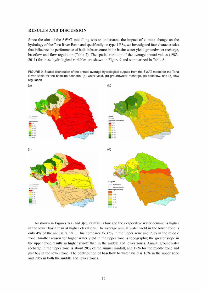
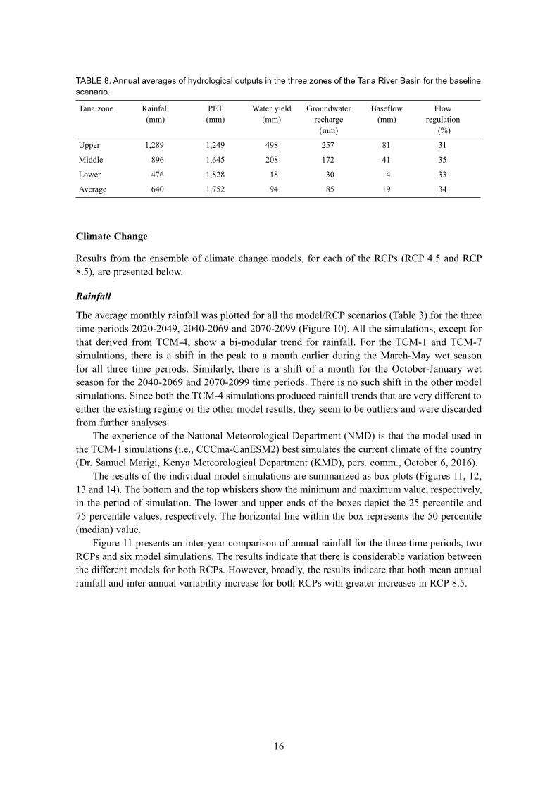
Since the aim of the SWAT modelling was to understand the impact of climate change on the hydrology of the Tana River Basin and specifically on type 1 ESs, we investigated four characteristics that influence the performance of built infrastructure in the basin: water yield, groundwater recharge, baseflow and flow regulation (Table 2). The spatial variation of the average annual values (1983-2011) for these hydrological variables are shown in Figure 9 and summarized in Table 8.

FIGURE 9. Spatial distribution of the annual average hydrological outputs from the SWAT model for the Tana River Basin for the baseline scenario. (a) water yield, (b) groundwater recharge, (c) baseflow, and (d) flow regulation.

(a) (b)

(c) (d)

As shown in Figures 2(a) and 3(c), rainfall is low and the evaporative water demand is higher in the lower basin than at higher elevations. The average annual water yield in the lower zone is only 4% of the annual rainfall. This compares to 37% in the upper zone and 23% in the middle zone. Another reason for higher water yield in the upper zone is topography; the greater slope in the upper zone results in higher runoff than in the middle and lower zones. Annual groundwater recharge in the upper zone is about 20% of the annual rainfall, and 19% for the middle zone and just 6% in the lower zone. The contribution of baseflow to water yield is 16% in the upper zone and 20% in both the middle and lower zones.

LegendRiver network

Sub-basin boundary

Flow regulation (%)0-15

15-25

25-35

35-40

40-50

>50

No data

16

TABLE 8. Annual averages of hydrological outputs in the three zones of the Tana River Basin for the baseline scenario.

Tana zone Rainfall PET Water yield Groundwater Baseflow Flow (mm) (mm) (mm) recharge (mm) regulation (mm) (%)

Upper 1,289 1,249 498 257 81 31

Middle 896 1,645 208 172 41 35

Lower 476 1,828 18 30 4 33

Average 640 1,752 94 85 19 34

climate change

Results from the ensemble of climate change models, for each of the RCPs (RCP 4.5 and RCP 8.5), are presented below.

Rainfall

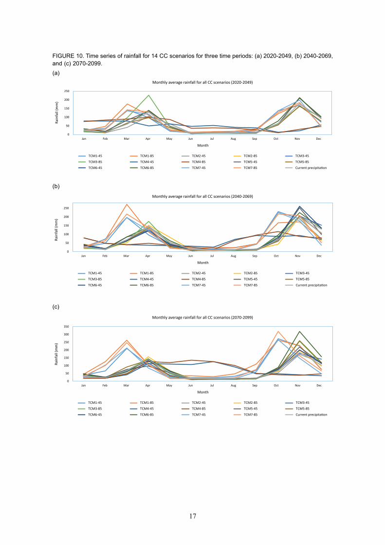
The average monthly rainfall was plotted for all the model/RCP scenarios (Table 3) for the three time periods 2020-2049, 2040-2069 and 2070-2099 (Figure 10). All the simulations, except for that derived from TCM-4, show a bi-modular trend for rainfall. For the TCM-1 and TCM-7 simulations, there is a shift in the peak to a month earlier during the March-May wet season for all three time periods. Similarly, there is a shift of a month for the October-January wet season for the 2040-2069 and 2070-2099 time periods. There is no such shift in the other model simulations. Since both the TCM-4 simulations produced rainfall trends that are very different to either the existing regime or the other model results, they seem to be outliers and were discarded from further analyses.

The experience of the National Meteorological Department (NMD) is that the model used in the TCM-1 simulations (i.e., CCCma-CanESM2) best simulates the current climate of the country (Dr. Samuel Marigi, Kenya Meteorological Department (KMD), pers. comm., October 6, 2016).

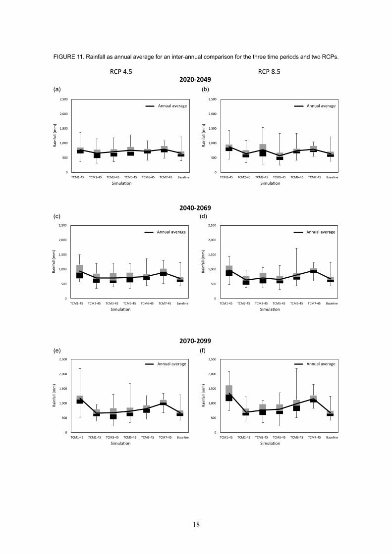
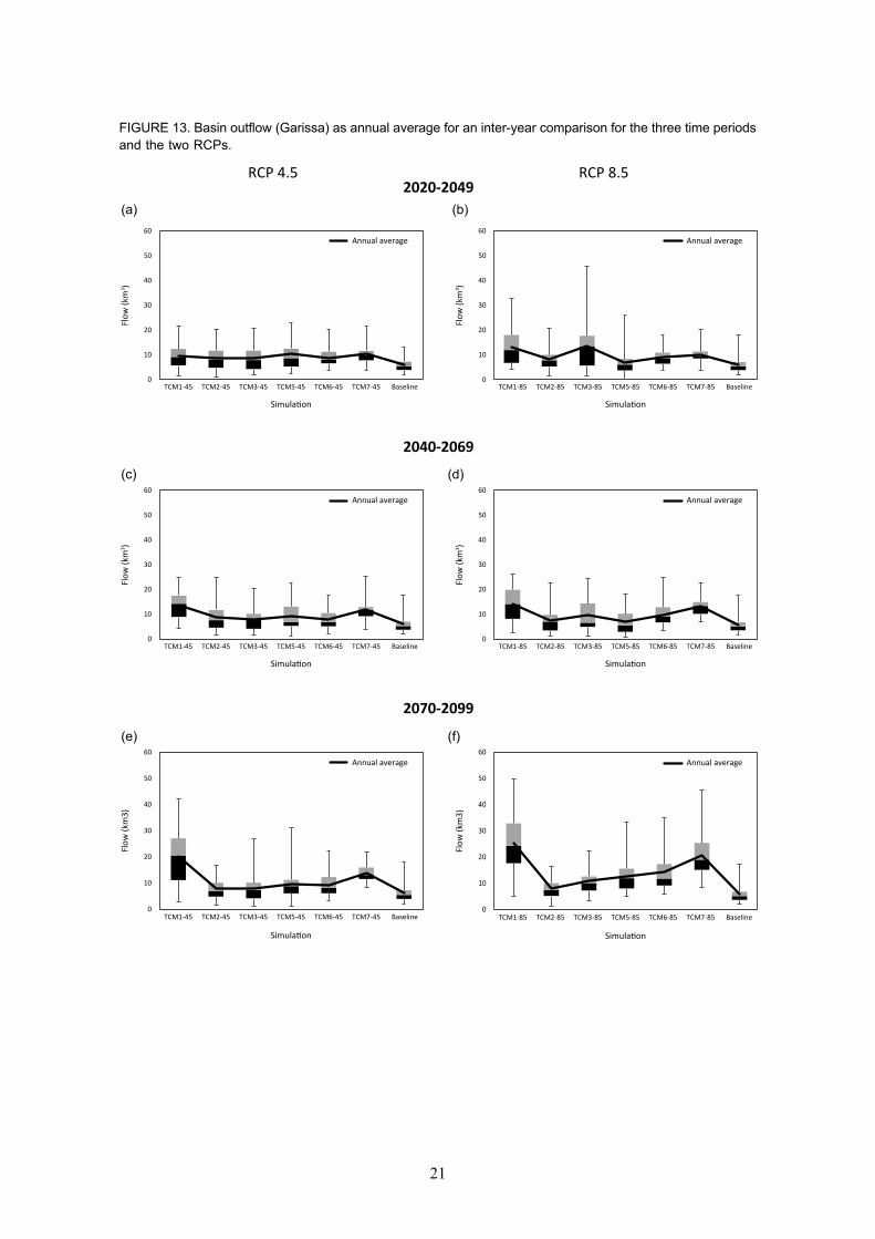
The results of the individual model simulations are summarized as box plots (Figures 11, 12, 13 and 14). The bottom and the top whiskers show the minimum and maximum value, respectively, in the period of simulation. The lower and upper ends of the boxes depict the 25 percentile and 75 percentile values, respectively. The horizontal line within the box represents the 50 percentile (median) value.

Figure 11 presents an inter-year comparison of annual rainfall for the three time periods, two RCPs and six model simulations. The results indicate that there is considerable variation between the different models for both RCPs. However, broadly, the results indicate that both mean annual rainfall and inter-annual variability increase for both RCPs with greater increases in RCP 8.5.

17

FIGURE 10. Time series of rainfall for 14 CC scenarios for three time periods: (a) 2020-2049, (b) 2040-2069, and (c) 2070-2099.(a)

(b)

(c)

0

50

100

150

200

250


Rain

fall

(mm

)

Month

Monthly average rainfall for all CC scenarios (2020-2049)

TCM1-45 TCM1-85 TCM2-45 TCM2-85 TCM3-45


TCM6-45 TCM6-85 TCM7-45 TCM7-85 Current precipitation

0

50

100

150

200

250


Rain

fall

(mm

)

Month






Rain

fall

(mm

)

Month





0

50

100

150

200

250

300

350

18

FIGURE 11. Rainfall as annual average for an inter-annual comparison for the three time periods and two RCPs.

(a) (b)

(c) (d)

(e) (f)

RCP 4.5 RCP 8.5

0

500

1,000

1,500

2,000

2,500

TCM1-45 TCM2-45 TCM3-45 TCM5-45 TCM6-45 TCM7-45 Baseline

Rain

fall

(mm

)

Simulation

Annual average

0

500

1,000

1,500

2,000

2,500


Rain

fall

(mm

)

Simulation

Annual average

2020-2049

0

500

1,000

1,500

2,000

2,500


Rain

fall

(mm

)

Simulation

Annual average

0

500

1,000

1,500

2,000

2,500


Rain

fall

(mm

)

Simulation

Annual average

2040-2069

0

500

1,000

1,500

2,000

2,500


Rain

fall

(mm

)

Annual average

0

500

1,000

1,500

2,000

2,500


Rain

fall

(mm

)

SimulationSimulation

Annual average

2070-2099

19

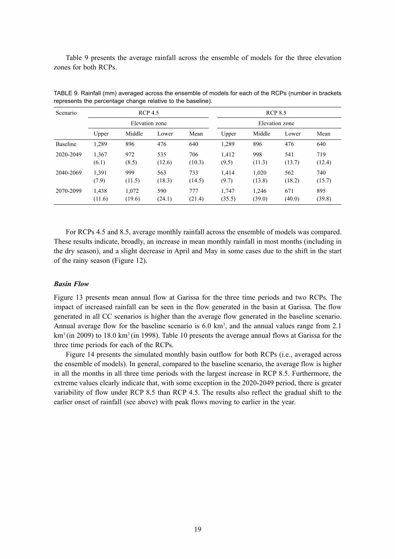
Table 9 presents the average rainfall across the ensemble of models for the three elevation zones for both RCPs.

For RCPs 4.5 and 8.5, average monthly rainfall across the ensemble of models was compared. These results indicate, broadly, an increase in mean monthly rainfall in most months (including in the dry season), and a slight decrease in April and May in some cases due to the shift in the start of the rainy season (Figure 12).

Basin Flow

Figure 13 presents mean annual flow at Garissa for the three time periods and two RCPs. The impact of increased rainfall can be seen in the flow generated in the basin at Garissa. The flow generated in all CC scenarios is higher than the average flow generated in the baseline scenario. Annual average flow for the baseline scenario is 6.0 km3, and the annual values range from 2.1 km3 (in 2009) to 18.0 km3 (in 1998). Table 10 presents the average annual flows at Garissa for the three time periods for each of the RCPs.

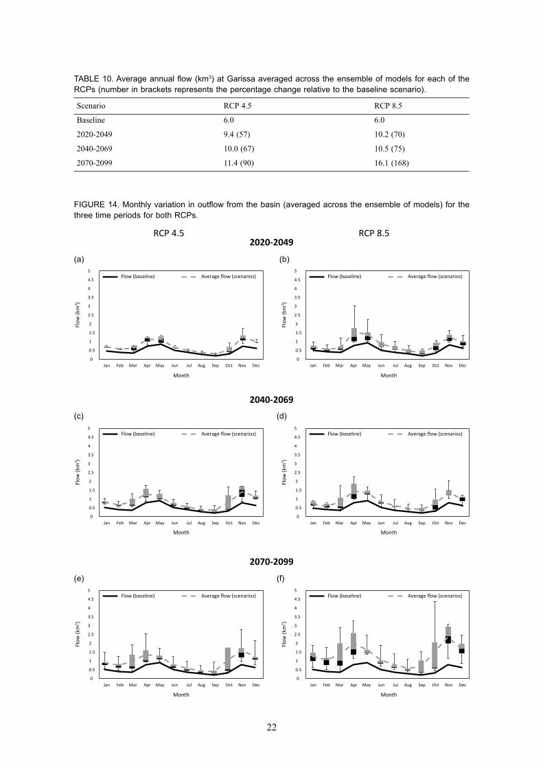
Figure 14 presents the simulated monthly basin outflow for both RCPs (i.e., averaged across the ensemble of models). In general, compared to the baseline scenario, the average flow is higher in all the months in all three time periods with the largest increase in RCP 8.5. Furthermore, the extreme values clearly indicate that, with some exception in the 2020-2049 period, there is greater variability of flow under RCP 8.5 than RCP 4.5. The results also reflect the gradual shift to the earlier onset of rainfall (see above) with peak flows moving to earlier in the year.

TABLE 9. Rainfall (mm) averaged across the ensemble of models for each of the RCPs (number in brackets represents the percentage change relative to the baseline).

Scenario RCP 4.5 RCP 8.5

Elevation zone Elevation zone

Upper Middle Lower Mean Upper Middle Lower Mean

Baseline 1,289 896 476 640 1,289 896 476 640

2020-2049 1,367 972 535 706 1,412 998 541 719 (6.1) (8.5) (12.6) (10.3) (9.5) (11.3) (13.7) (12.4)

2040-2069 1,391 999 563 733 1,414 1,020 562 740 (7.9) (11.5) (18.3) (14.5) (9.7) (13.8) (18.2) (15.7)

2070-2099 1,438 1,072 590 777 1,747 1,246 671 895 (11.6) (19.6) (24.1) (21.4) (35.5) (39.0) (40.0) (39.8)

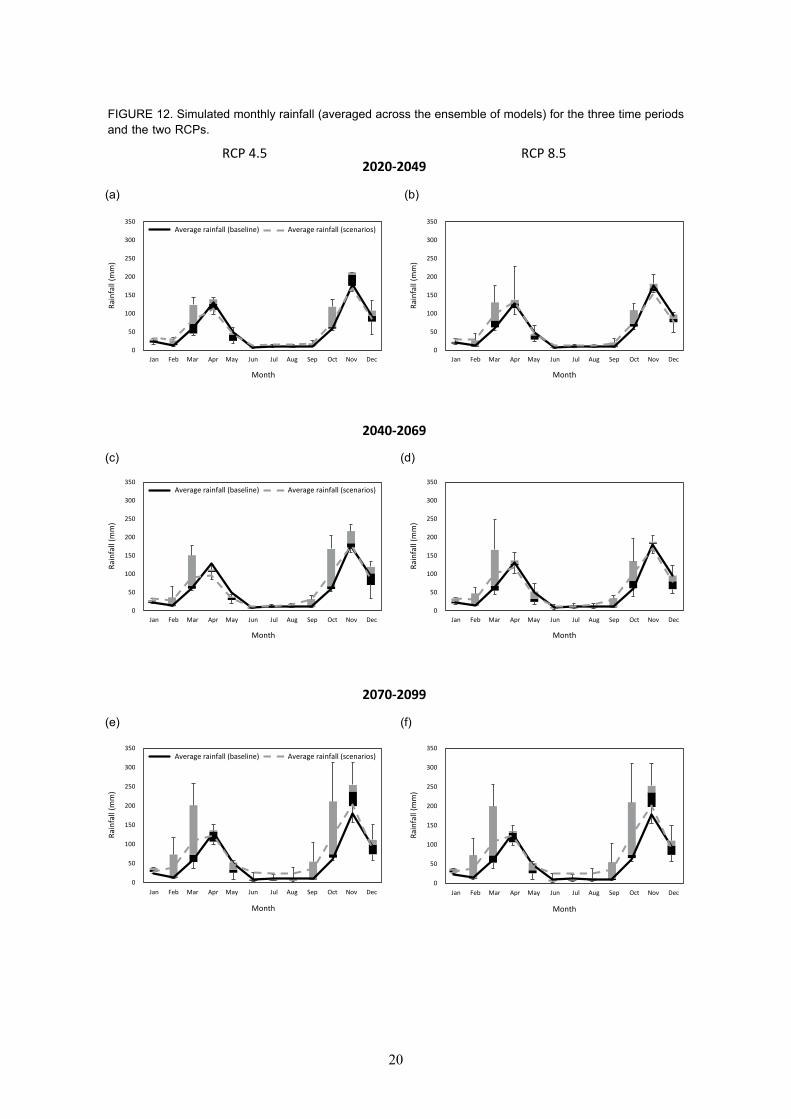
20

FIGURE 12. Simulated monthly rainfall (averaged across the ensemble of models) for the three time periods and the two RCPs.

0

50

100

150

200

250

300

350


Rain

fall

(mm

)

Month Month

Average rainfall (baseline) Average rainfall (scenarios)

0

50

100

150

200

250

300

350


Rain

fall

(mm

)

RCP 4.5 RCP 8.52020-2049

0

50

100

150

200

250

300

350


Rain

fall

(mm

)

Month Month


0

50

100

150

200

250

300

350


Rain

fall

(mm

)

2040-2069

0

50

100

150

200

250

300

350


Rain

fall

(mm

)

Month Month


0

50

100

150

200

250

300

350


Rain

fall

(mm

)

2070-2099

(a) (b)

(c) (d)

(e) (f)

21

(a) (b)

(c) (d)

(e) (f)

FIGURE 13. Basin outflow (Garissa) as annual average for an inter-year comparison for the three time periods and the two RCPs.

0

10

20

30

40

50

60


Flow

(km

3 )

Simulation

Annual average

0

10

20

30

40

50

60


Flow

(km

3 )

Simulation

Annual average

RCP 4.5 RCP 8.52020-2049

0

10

20

30

40

50

60


Flow

(km

3 )

Simulation

Annual average

0

10

20

30

40

50

60


Flow

(km

3 )

Simulation

Annual average

2040-2069

0

10

20

30

40

50

60


Flow

(km

3)

Simulation

Annual average

0

10

20

30

40

50

60


Flow

(km

3)

Simulation

Annual average

2070-2099

22

TABLE 10. Average annual flow (km3) at Garissa averaged across the ensemble of models for each of the RCPs (number in brackets represents the percentage change relative to the baseline scenario).

Scenario RCP 4.5 RCP 8.5

Baseline 6.0 6.0

2020-2049 9.4 (57) 10.2 (70)

2040-2069 10.0 (67) 10.5 (75)

2070-2099 11.4 (90) 16.1 (168)

FIGURE 14. Monthly variation in outflow from the basin (averaged across the ensemble of models) for the three time periods for both RCPs.

0

2

1.5

1

0.5

2.5

3

3.5

4

4.5

5


Flow

(km

3 )

Flow (baseline) Average flow (scenarios)

RCP 4.5 RCP 8.52020-2049

0

2

1.5

1

0.5

2.5

3

3.5

4

4.5

5


Flow

(km

3 )Flow (baseline) Average flow (scenarios)

0

2

1.5

1

0.5

2.5

3

3.5

4

4.5

5


Flow

(km

3 )


2040-2069

0

2

1.5

1

0.5

2.5

3

3.5

4

4.5

5


Flow

(km

3 )


0

2

1.5

1

0.5

2.5

3

3.5

4

4.5

5


Flow

(km

3 )


2070-2099

0

2

1.5

1

0.5

2.5

3

3.5

4

4.5

5


Flow

(km

3 )


Month Month

Month Month

Month Month

(a) (b)

(c) (d)

(e) (f)

23

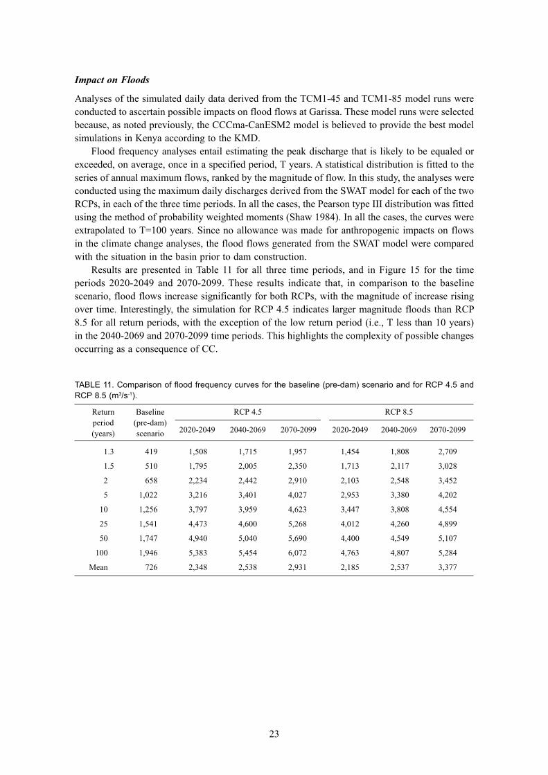
Impact on Floods

Analyses of the simulated daily data derived from the TCM1-45 and TCM1-85 model runs were conducted to ascertain possible impacts on flood flows at Garissa. These model runs were selected because, as noted previously, the CCCma-CanESM2 model is believed to provide the best model simulations in Kenya according to the KMD.

Flood frequency analyses entail estimating the peak discharge that is likely to be equaled or exceeded, on average, once in a specified period, T years. A statistical distribution is fitted to the series of annual maximum flows, ranked by the magnitude of flow. In this study, the analyses were conducted using the maximum daily discharges derived from the SWAT model for each of the two RCPs, in each of the three time periods. In all the cases, the Pearson type III distribution was fitted using the method of probability weighted moments (Shaw 1984). In all the cases, the curves were extrapolated to T=100 years. Since no allowance was made for anthropogenic impacts on flows in the climate change analyses, the flood flows generated from the SWAT model were compared with the situation in the basin prior to dam construction.

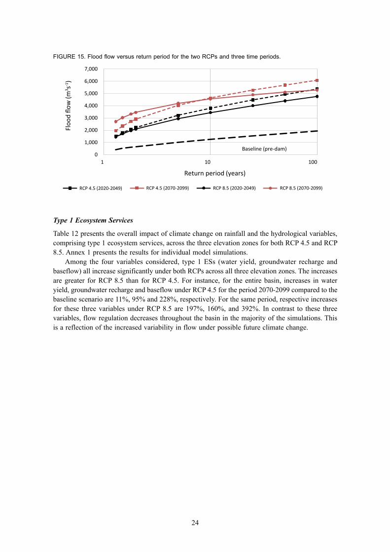
Results are presented in Table 11 for all three time periods, and in Figure 15 for the time periods 2020-2049 and 2070-2099. These results indicate that, in comparison to the baseline scenario, flood flows increase significantly for both RCPs, with the magnitude of increase rising over time. Interestingly, the simulation for RCP 4.5 indicates larger magnitude floods than RCP 8.5 for all return periods, with the exception of the low return period (i.e., T less than 10 years) in the 2040-2069 and 2070-2099 time periods. This highlights the complexity of possible changes occurring as a consequence of CC.

TABLE 11. Comparison of flood frequency curves for the baseline (pre-dam) scenario and for RCP 4.5 and RCP 8.5 (m3/s-1).

RCP 4.5 RCP 8.5

1.3 419 1,508 1,715 1,957 1,454 1,808 2,709

1.5 510 1,795 2,005 2,350 1,713 2,117 3,028

2 658 2,234 2,442 2,910 2,103 2,548 3,452

5 1,022 3,216 3,401 4,027 2,953 3,380 4,202

10 1,256 3,797 3,959 4,623 3,447 3,808 4,554

25 1,541 4,473 4,600 5,268 4,012 4,260 4,899

50 1,747 4,940 5,040 5,690 4,400 4,549 5,107

100 1,946 5,383 5,454 6,072 4,763 4,807 5,284

Mean 726 2,348 2,538 2,931 2,185 2,537 3,377

Return Baseline period (pre-dam) (years) scenario 2020-2049 2040-2069 2070-2099 2020-2049 2040-2069 2070-2099

24

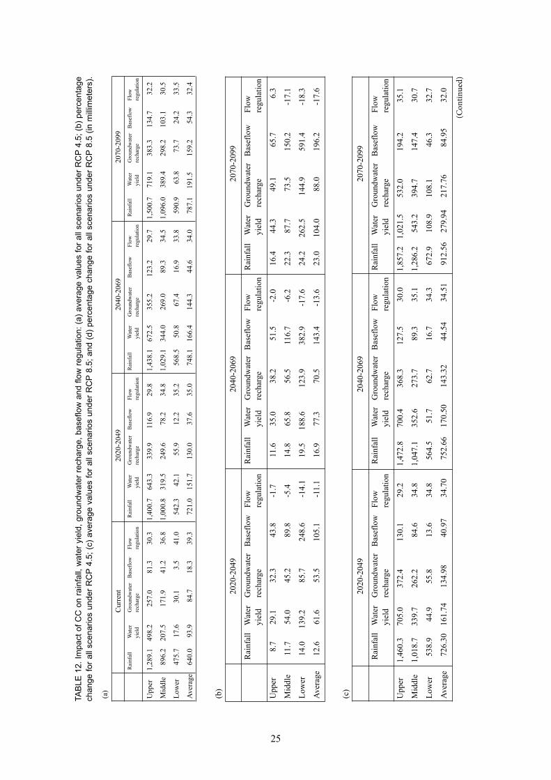
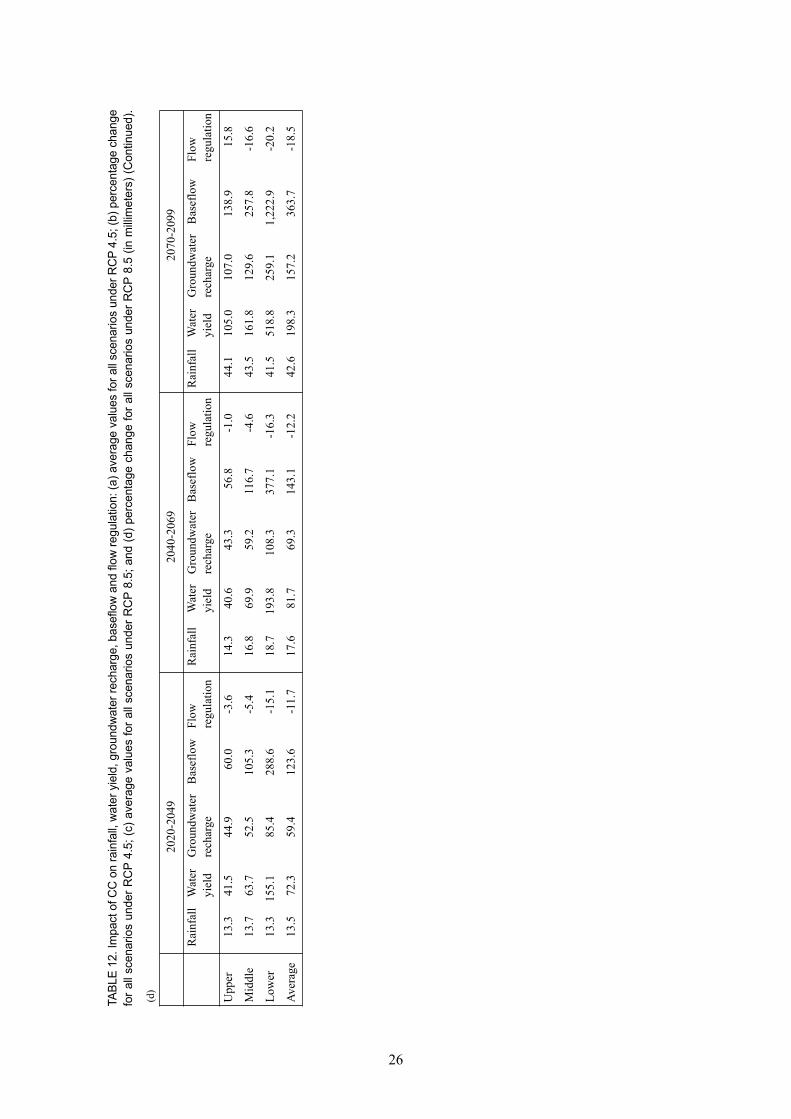
Type 1 Ecosystem Services

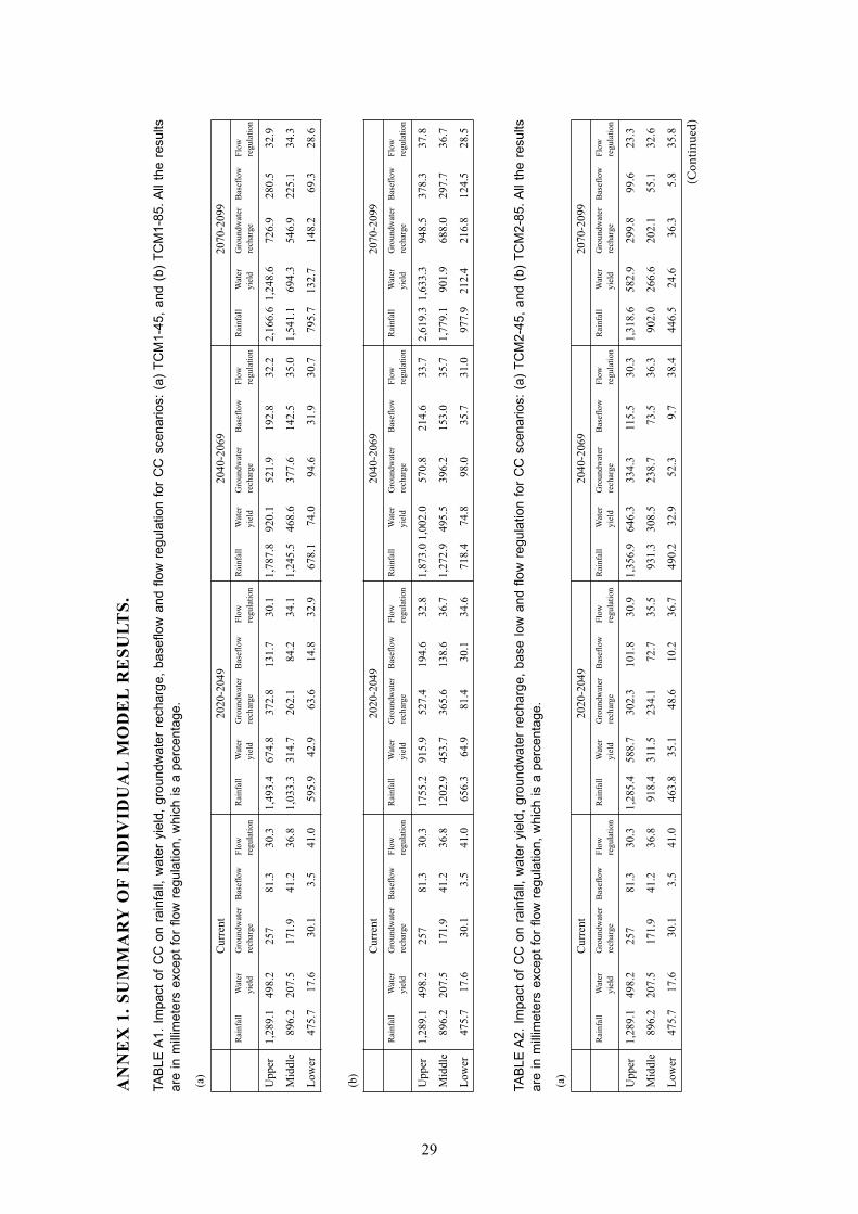
Table 12 presents the overall impact of climate change on rainfall and the hydrological variables, comprising type 1 ecosystem services, across the three elevation zones for both RCP 4.5 and RCP 8.5. Annex 1 presents the results for individual model simulations.

Among the four variables considered, type 1 ESs (water yield, groundwater recharge and baseflow) all increase significantly under both RCPs across all three elevation zones. The increases are greater for RCP 8.5 than for RCP 4.5. For instance, for the entire basin, increases in water yield, groundwater recharge and baseflow under RCP 4.5 for the period 2070-2099 compared to the baseline scenario are 11%, 95% and 228%, respectively. For the same period, respective increases for these three variables under RCP 8.5 are 197%, 160%, and 392%. In contrast to these three variables, flow regulation decreases throughout the basin in the majority of the simulations. This is a reflection of the increased variability in flow under possible future climate change.

FIGURE 15. Flood flow versus return period for the two RCPs and three time periods.

0

1,000

2,000

3,000

4,000

5,000

6,000

7,000

1 10 100

Floo

d flo

w (m

3 s-1)

Return period (years)

RCP 4.5 (2020-2049) RCP 4.5 (2070-2099) RCP 8.5 (2020-2049) RCP 8.5 (2070-2099)

Baseline (pre-dam)

25

TABL

E 12

. Im

pact

of C

C o

n ra

infa

ll, w

ater

yie

ld, g

roun

dwat

er re

char

ge, b

asef

low

and

flow

regu

latio

n: (a

) ave

rage

val

ues

for a

ll sc

enar

ios

unde

r RC

P 4.

5; (b

) per

cent

age

chan

ge fo

r all

scen

ario

s un

der R

CP

4.5;

(c) a

vera

ge v

alue

s fo

r all

scen

ario

s un

der R

CP

8.5;

and

(d) p

erce

ntag

e ch

ange

for a

ll sc

enar

ios

unde

r RC

P 8.

5 (in

milli

met

ers)

.

(a)

C

urre

nt

2020

-204

9 20

40-2

069

2070

-209

9

Rai

nfal

l W

ater

G

roun

dwat

er

Bas

eflo

w

Flow

R

ainf

all

Wat

er

Gro

undw

ater

B

asef

low

Fl

ow

Rai

nfal

l W

ater

G

roun

dwat

er

Bas

eflo

w

Flow

R

ainf

all

Wat

er

Gro

undw

ater

B

asef

low

Fl

ow

yiel

d re

char

ge

re

gula

tion

yi

eld

rech

arge

regu

latio

n

yiel

d re

char

ge

re

gula

tion

yi

eld

rech

arge

regu

latio

n

Upp

er

1,28

9.1

498.

2 25

7.0

81.3

30

.3

1,40

0.7

643.

3 33

9.9

116.

9 29

.8

1,43

8.1

672.

5 35

5.2

123.

2 29

.7

1,50

0.7

719.

1 38

3.3

134.

7 32

.2

Mid

dle

896.

2 20

7.5

171.

9 41

.2

36.8

1,

000.

8 31

9.5

249.

6 78

.2

34.8

1,

029.

1 34

4.0

269.

0 89

.3

34.5

1,

096.

0 38

9.4

298.

2 10

3.1

30.5

Low

er

475.

7 17

.6

30.1

3.

5 41

.0

542.

3 42

.1

55.9

12

.2

35.2

56

8.5

50.8

67

.4

16.9

33

.8

590.

9 63

.8

73.7

24

.2

33.5

Aver

age

640.

0 93

.9

84.7

18

.3

39.3

72

1.0

151.

7 13

0.0

37.6

35

.0

748.

1 16

6.4

144.

3 44

.6

34.0

78

7.1

191.

5 15

9.2

54.3

32

.4

(b)

20

20-2

049

2040

-206

9 20

70-2

099

R

ainf

all

Wat

er

Gro

undw

ater

B

asef

low

Fl

ow

Rai

nfal

l W

ater

G

roun

dwat

er

Bas

eflo

w

Flow

R

ainf

all

Wat

er

Gro

undw

ater

B

asef

low

Fl

ow

yiel

d re

char

ge

re

gula

tion

yi

eld

rech

arge

regu

latio

n

yiel

d re

char

ge

re

gula

tion

Upp

er

8.7

29.1

32

.3

43.8

-1

.7

11.6

35

.0

38.2

51

.5

-2.0

16

.4

44.3

49

.1

65.7

6.

3

Mid

dle

11.7

54

.0

45.2

89

.8

-5.4

14

.8

65.8

56

.5

116.

7 -6

.2

22.3

87

.7

73.5

15

0.2

-17.

1

Low

er

14.0

13

9.2

85.7

24

8.6

-14.

1 19

.5

188.

6 12

3.9

382.

9 -1

7.6

24.2

26

2.5

144.

9 59

1.4

-18.

3

Aver

age

12.6

61

.6

53.5

10

5.1

-11.

1 16

.9

77.3

70

.5

143.

4 -1

3.6

23.0

10

4.0

88.0

19

6.2

-17.

6

(c)

20

20-2

049

2040

-206

9 20

70-2

099

R

ainf

all

Wat

er

Gro

undw

ater

B

asef

low

Fl

ow

Rai

nfal

l W

ater

G

roun

dwat

er

Bas

eflo

w

Flow

R

ainf

all

Wat

er

Gro

undw

ater

B

asef

low

Fl

ow

yiel

d re

char

ge

re

gula

tion

yi

eld

rech

arge

regu

latio

n

yiel

d re

char

ge

re

gula

tion

Upp

er

1,46

0.3

705.

0 37

2.4

130.

1 29

.2

1,47

2.8

700.

4 36

8.3

127.

5 30

.0

1,85

7.2

1,02

1.5

532.

0 19

4.2

35.1

Mid

dle

1,01

8.7

339.

7 26

2.2

84.6

34

.8

1,04

7.1

352.

6 27

3.7

89.3

35

.1

1,28

6.2

543.

2 39

4.7

147.

4 30

.7

Low

er

538.

9 44

.9

55.8

13

.6

34.8

56

4.5

51.7

62

.7

16.7

34

.3

672.

9 10

8.9

108.

1 46

.3

32.7

Aver

age

726.

30

161.

74

134.

98

40.9

7 34

.70

752.

66

170.

50

143.

32

44.5

4 34

.51

912.

56

279.

94

217.

76

84.9

5 32

.0

(Con

tinued)

26

TABL

E 12

. Im

pact

of C

C o

n ra

infa

ll, w

ater

yie

ld, g

roun

dwat

er re

char

ge, b

asef

low

and

flow

regu

latio

n: (a

) ave

rage

val

ues

for a

ll sc

enar

ios

unde

r RC

P 4.

5; (b

) per

cent

age

chan

ge

for a

ll sc

enar

ios

unde

r RC

P 4.

5; (c

) ave

rage

val

ues

for a

ll sc

enar

ios

unde

r RC

P 8.

5; a

nd (d

) per

cent

age

chan

ge fo

r all

scen

ario

s un

der R

CP

8.5

(in m

illim

eter

s) (C

ontin

ued)

.

(d)

20

20-2

049

2040

-206

9 20

70-2

099

R

ainf

all

Wat

er

Gro

undw

ater

B

asef

low

Fl

ow

Rai

nfal

l W

ater

G

roun

dwat

er

Bas

eflo

w

Flow

R

ainf

all

Wat

er

Gro

undw

ater

B

asef

low

Fl

ow

yiel

d re

char

ge

re

gula

tion

yi

eld

rech

arge

regu

latio

n

yiel

d re

char

ge

re

gula

tion

Upp

er

13.3

41

.5

44.9

60

.0

-3.6

14

.3

40.6

43

.3

56.8

-1

.0

44.1

10

5.0

107.

0 13

8.9

15.8

Mid

dle

13.7

63

.7

52.5

10

5.3

-5.4

16

.8

69.9

59

.2

116.

7 -4

.6

43.5

16

1.8

129.

6 25

7.8

-16.

6

Low

er

13.3

15

5.1

85.4

28

8.6

-15.

1 18

.7

193.

8 10

8.3

377.

1 -1

6.3

41.5

51

8.8

259.

1 1,

222.

9 -2

0.2

Aver

age

13.5

72

.3

59.4

12

3.6

-11.

7 17

.6

81.7

69

.3

143.

1 -1

2.2

42.6

19

8.3

157.

2 36

3.7

-18.

5

27

concluSIon

A hydrological model, SWAT, was setup for the Tana River Basin in Kenya to generate outputs from an ensemble of climate models under RCP 4.5 and RCP 8.5. Results derived for three future time periods, 2020-2049, 2040-2069 and 2070-2099, were compared to a 1983-2011 baseline.

The results confirm the findings of others that there will likely be a reversal of recent historic trends of declining rainfall. Rather, rainfall is projected to increase across the basin over the remainder of the twenty-first century, with greater increases (up to 40% by the end of the century) under RCP 8.5 than RCP 4.5. The results also indicate an earlier onset of rainfall for both the long and the short rainy season under both RCPs.

A consequence of the increased rainfall is disproportionate increases in flow from the basin. The mean annual flow at Garissa increases significantly by 90% under RCP 4.5 and more than doubles under RCP 8.5 by the end of the twenty-first century. Flood flows and variability are also projected to increase significantly under both RCPs.

The modeling results indicate significant changes in type 1 ecosystem services. The impact of climate change on water yield, groundwater recharge, base flow and flow regulation were estimated. The first three variables (water yield, groundwater recharge and baseflow) progressively increase under both RCPs, but with greater increases under RCP 8.5 than 4.5. In contrast, natural flow regulation reduces across most of the basin in most future time periods, resulting in increased seasonal variability in flows and larger floods. The reductions in flow regulation are comparable under both RCPs.

Increases in rainfall and flow broadly indicate an improved water resource situation in the future, with opportunities for increasing benefits from built infrastructure (i.e., hydropower generation as well as irrigation and water supply diversions). However, declining natural flow regulation, increased variability, and significant increases in the frequency and magnitude of floods pose a significant risk that threatens to undermine development opportunities. Water resources management is likely to be more difficult than under historic climatic conditions. To build resilience, water resource managers need to adapt to changing conditions. Though working with natural processes is currently a challenge, better understanding of the role of natural infrastructure and explicit integration of type 1 ecosystem service will likely be a prerequisite for sustainable water resources management in the future.

28

referenceS

Abbaspour, K.C. 2011. SWAT-CUP4: SWAT Calibration and Uncertainty Programs: A user manual. Dübendorf, Switzerland: Department of Systems Analysis, Integrated Assessment Modelling (SIAM), Swiss Federal Institute of Aquatic Science and Technology (Eawag).

Abbaspour, K.C.; Yang, J.; Maximov, I.; Siber, R.; Bogner, K.; Mieleitner, J.; Zobrist, J.; Srinivasan, R. 2007. Modelling hydrology and water quality in the pre-alpine/alpine Thur watershed using SWAT. Journal of Hydrology 333(2-4): 413-430.

Arnold, J.G.; Srinivasan, R.; Muttiah, R.S.; Williams, J.R. 1998. Large area hydrologic modeling and assessment Part 1: Model development. Journal of the American Water Resources Association 34(1): 73-89.

Droogers, P.; Butterfield, R.; Dyszynski, J. 2009. Climate change and hydropower impact and adaptation costs: Case study Kenya. FutureWater Report 85. Wageningen, The Netherlands: FutureWater.

FAO (Food and Agriculture Organization of the United Nations); UNESCO (United Nations Educational, Scientific and Cultural Organization). 1995. The digital soil map of the world. Rome, Italy: Food and Agriculture Organization of the United Nations (FAO); Paris, France: United Nations Educational, Scientific and Cultural Organization (UNESCO).

Giorgi, F.; Gutowski, W.J. 2016. Coordinated experiments for projections of regional climate change. Current Climate Change Reports 2(4): 202-210.

GoK (Government of Kenya). 2012. National climate change action plan 2013-2017. Nairobi, Kenya: Ministry of Environment and Mineral Resources.

Leauthaud, C.; Belaud, G.; Duvail, S.; Moussa, R.; Grünberger, O.; Albergel, J. 2013. Characterizing floods in the poorly gauged wetlands of the Tana River Delta, Kenya, using a water balance model and satellite data. Hydrology and Earth System Sciences 17(8): 3059-3075.

McCartney, M.P.; Foudi, S.; Muthuwatta, L.; Sood, A.; Simons, G.; Hunink, J.; Vercruysse, K. Forthcoming. Water, natural and built infrastructure and ecosystem services in the Tana River Basin. Colombo, Sri Lanka: International Water Management Institute (IWMI). (IWMI Research Report).

Nakaegawa, T.; Wachana, C.; KAKUSHIN Team-3 Modeling Group. 2012. First impact assessment of hydrological cycle in the Tana River Basin, Kenya, under a changing climate in the late 21st century. Hydrological Research Letters 6: 29-34.

Nash, J.E.; Sutcliffe, J.V. 1970. River flow forecasting through conceptual models part I - A discussion of principles. Journal of Hydrology 10(3): 282-290.

Oates, N.; Marani, M. 2017. Making water infrastructure investment decisions in a changing climate: A political economy study of river basin development in Kenya. London, UK: Overseas Development Institute (ODI).

Shaw, E.M. 1984. Hydrology in Practice. Wokingham, UK: Van Nostrand Reinhold (UK) Ltd.

Sood, A.; Muthuwatta, L.; McCartney, M.P. 2013. Evaluating the effect of possible climate change on the hydrology of the Volta River Basin using the SWAT model. Water International 38(3): 297-311.

van Vuuren, D.P.; Edmonds, J.; Kainuma, M.; Riahi, K.; Thomson, A.; Hibbard, K.; Hurtt, G.C.; Kram, T.; Krey, V.; Lamarque, J-F.; Masui, T.; Meinshausen, M.; Nakicenovic, N.; Smith, S.J.; Rose, S.K. 2011. The representative concentration pathways: An overview. Climate Change 109: 5-31.

Wamuongo, J.; Okoti, M.; Mwara, J.; Isako, T. 2014. Piloting and upscaling appropriate adaptation strategies for resilience building in the ASALs of Kenya. Final report for Agricultural Productivity and Climate Change in Arid and Semi Arid Kenya. Nairobi, Kenya: Kenya Agricultural and Livestock Research Organization.

29

(Con

tinued)

An

ne

x 1

. Su

MM

Ar

y o

f In

dIV

Idu

Al

Mo

de

l r

eSu

ltS.

TABL

E A1

. Im

pact

of C

C o

n ra

infa

ll, w

ater

yie

ld, g

roun

dwat

er r

echa

rge,

bas

eflo

w a

nd fl

ow r

egul

atio

n fo

r C

C s

cena

rios:

(a)

TC

M1-

45, a

nd (

b) T

CM

1-85

. All

the

resu

lts

are

in m

illim

eter

s ex

cept

for f

low

regu

latio

n, w

hich

is a

per

cent

age.

(a)

C

urre

nt

2020

-204

9 20

40-2

069

2070

-209

9

Rai

nfal

l W

ater

G

roun

dwat

er

Bas

eflo

w

Flow

R

ainf

all

Wat

er

Gro

undw

ater

B

asef

low

Fl

ow

Rai

nfal

l W

ater

G

roun

dwat

er

Bas

eflo

w

Flow

R

ainf

all

Wat

er

Gro

undw

ater

B

asef

low

Fl

ow

yiel

d re

char

ge

re

gula

tion

yi

eld

rech

arge

regu

latio

n

yiel

d re

char

ge

re

gula

tion

yi

eld

rech

arge

regu

latio

n

Upp

er

1,28

9.1

498.

2 25

7 81

.3

30.3

1,

493.

4 67

4.8

372.

8 13

1.7

30.1

1,

787.

8 92

0.1

521.

9 19

2.8

32.2

2,

166.

6 1,

248.

6 72

6.9

280.

5 32

.9

Mid

dle

896.

2 20

7.5

171.

9 41

.2

36.8

1,

033.

3 31

4.7

262.

1 84

.2

34.1

1,

245.

5 46

8.6

377.

6 14

2.5

35.0

1,

541.

1 69

4.3

546.

9 22

5.1

34.3

Low

er

475.

7 17

.6

30.1

3.

5 41

.0

595.

9 42

.9

63.6

14

.8

32.9

67

8.1

74.0

94

.6

31.9

30

.7

795.

7 13

2.7

148.

2 69

.3

28.6

(b)

C

urre

nt

2020

-204

9 20

40-2

069

2070

-209

9

Rai

nfal

l W

ater

G

roun

dwat

er

Bas

eflo

w

Flow

R

ainf

all

Wat

er

Gro

undw

ater

B

asef

low

Fl

ow

Rai

nfal

l W

ater

G

roun

dwat

er

Bas

eflo

w

Flow

R

ainf

all

Wat

er

Gro

undw

ater

B

asef

low

Fl

ow

yiel

d re

char

ge

re

gula

tion

yi

eld

rech

arge

regu

latio

n

yiel

d re

char

ge

re

gula

tion

yi

eld

rech

arge

regu

latio

n

Upp

er

1,28

9.1

498.

2 25

7 81

.3

30.3

17

55.2

91

5.9

527.

4 19

4.6

32.8

1,

873.

0 1,

002.

0 57

0.8

214.

6 33

.7

2,61

9.3

1,63

3.3

948.

5 37

8.3

37.8

Mid

dle

896.

2 20

7.5

171.

9 41

.2

36.8

12

02.9

45

3.7

365.

6 13

8.6

36.7

1,

272.

9 49

5.5

396.

2 15

3.0

35.7

1,

779.

1 90

1.9

688.

0 29

7.7

36.7

Low

er

475.

7 17

.6

30.1

3.

5 41

.0

656.

3 64

.9

81.4

30

.1

34.6

71

8.4

74.8

98

.0

35.7

31

.0

977.

9 21

2.4

216.

8 12

4.5

28.5

TABL

E A2

. Im

pact

of C

C o

n ra

infa

ll, w

ater

yie

ld, g

roun

dwat

er r

echa

rge,

bas

e lo

w a

nd fl

ow r

egul

atio

n fo

r C

C s

cena

rios:

(a)

TC

M2-

45, a

nd (

b) T

CM

2-85

. All

the

resu

lts

are

in m

illim

eter

s ex

cept

for f

low

regu

latio

n, w

hich

is a

per

cent

age.

(a)

C

urre

nt

2020

-204

9 20

40-2

069

2070

-209

9

Rai

nfal

l W

ater

G

roun

dwat

er

Bas

eflo

w

Flow

R

ainf

all

Wat

er

Gro

undw

ater

B

asef

low

Fl

ow

Rai

nfal

l W

ater

G

roun

dwat

er

Bas

eflo

w

Flow

R

ainf

all

Wat

er

Gro

undw

ater

B

asef

low

Fl

ow

yiel

d re

char

ge

re

gula

tion

yi

eld

rech

arge

regu

latio

n

yiel

d re

char

ge

re

gula

tion

yi

eld

rech

arge

regu

latio

n

Upp

er

1,28

9.1

498.

2 25

7 81

.3

30.3

1,

285.

4 58

8.7

302.

3 10

1.8

30.9

1,

356.

9 64

6.3

334.

3 11

5.5

30.3

1,

318.

6 58

2.9

299.

8 99

.6

23.3

Mid

dle

896.

2 20

7.5

171.

9 41

.2

36.8

91

8.4

311.

5 23

4.1

72.7

35

.5

931.

3 30

8.5

238.

7 73

.5

36.3

90

2.0

266.

6 20

2.1

55.1

32

.6

Low

er

475.

7 17

.6

30.1

3.

5 41

.0

463.

8 35

.1

48.6

10

.2

36.7

49

0.2

32.9

52

.3

9.7

38.4

44

6.5

24.6

36

.3

5.8

35.8

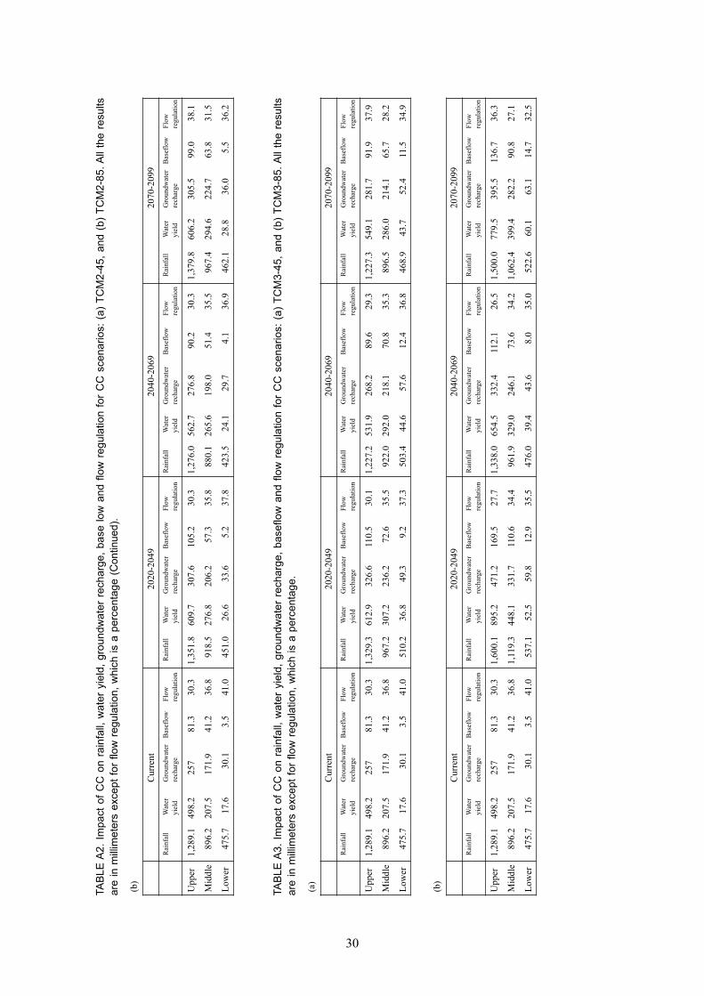
30

TABL

E A2

. Im

pact

of C

C o

n ra

infa

ll, w

ater

yie

ld, g

roun

dwat

er r

echa

rge,

bas

e lo

w a

nd fl

ow r

egul

atio

n fo

r C

C s

cena

rios:

(a)

TC

M2-

45, a

nd (

b) T

CM

2-85

. All

the

resu

lts

are

in m

illim

eter

s ex

cept

for f

low

regu

latio

n, w

hich

is a

per

cent

age

(Con

tinue

d).

(b)

C

urre

nt

2020

-204

9 20

40-2

069

2070

-209

9

Rai

nfal

l W

ater

G

roun

dwat

er

Bas

eflo

w

Flow

R

ainf

all

Wat

er

Gro

undw

ater

B

asef

low

Fl

ow

Rai

nfal

l W

ater

G

roun

dwat

er

Bas

eflo

w

Flow

R

ainf

all

Wat

er

Gro

undw

ater

B

asef

low

Fl

ow

yiel

d re

char

ge

re

gula

tion

yi

eld

rech

arge

regu

latio

n

yiel

d re

char

ge

re

gula

tion

yi

eld

rech

arge

regu

latio

n

Upp

er

1,28

9.1

498.

2 25

7 81

.3

30.3

1,

351.

8 60

9.7

307.

6 10

5.2

30.3

1,

276.

0 56

2.7

276.

8 90

.2

30.3

1,

379.

8 60

6.2

305.

5 99

.0

38.1

Mid

dle

896.

2 20

7.5

171.

9 41

.2

36.8

91

8.5

276.

8 20

6.2

57.3

35

.8

880.

1 26

5.6

198.

0 51

.4

35.5

96

7.4

294.

6 22

4.7

63.8

31

.5

Low

er

475.

7 17

.6

30.1

3.

5 41

.0

451.

0 26

.6

33.6

5.

2 37

.8

423.

5 24

.1

29.7

4.

1 36

.9

462.

1 28

.8

36.0

5.

5 36

.2

TABL

E A3

. Im

pact

of C

C o

n ra

infa

ll, w

ater

yie

ld, g

roun

dwat

er r

echa

rge,

bas

eflo

w a

nd fl

ow r

egul

atio

n fo

r C

C s

cena

rios:

(a)

TC

M3-

45, a

nd (

b) T

CM

3-85

. All

the

resu

lts

are

in m

illim

eter

s ex

cept

for f

low

regu

latio

n, w

hich

is a

per

cent

age.

(a)

C

urre

nt

2020

-204

9 20

40-2

069

2070

-209

9

Rai

nfal

l W

ater

G

roun

dwat

er

Bas

eflo

w

Flow

R

ainf

all

Wat

er

Gro

undw

ater

B

asef

low

Fl

ow

Rai

nfal

l W

ater

G

roun

dwat

er

Bas

eflo

w

Flow

R

ainf

all

Wat

er

Gro

undw

ater

B

asef

low

Fl

ow

yiel

d re

char

ge

re

gula

tion

yi

eld

rech

arge

regu

latio

n

yiel

d re

char

ge

re

gula

tion

yi

eld

rech

arge

regu

latio

n

Upp

er

1,28

9.1

498.

2 25

7 81

.3

30.3

1,

329.

3 61

2.9

326.

6 11

0.5

30.1

1,

227.

2 53

1.9

268.

2 89

.6

29.3

1,

227.

3 54

9.1

281.

7 91

.9

37.9

Mid

dle

896.

2 20

7.5

171.

9 41

.2

36.8

96

7.2

307.

2 23

6.2

72.6

35

.5

922.

0 29

2.0

218.

1 70

.8

35.3

89

6.5

286.

0 21

4.1

65.7

28

.2

Low

er

475.

7 17

.6

30.1

3.

5 41

.0

510.

2 36

.8

49.3

9.

2 37

.3

503.

4 44

.6

57.6

12

.4

36.8

46

8.9

43.7

52

.4

11.5

34

.9

(b)

C

urre

nt

2020

-204

9 20

40-2

069

2070

-209

9

Rai

nfal

l W

ater

G

roun

dwat

er

Bas

eflo

w

Flow

R

ainf

all

Wat

er

Gro

undw

ater

B

asef

low

Fl

ow

Rai

nfal

l W

ater

G

roun

dwat

er

Bas

eflo

w

Flow

R

ainf

all

Wat

er

Gro

undw

ater

B

asef

low

Fl

ow

yiel

d re

char

ge

re

gula

tion

yi

eld

rech

arge

regu

latio

n

yiel

d re

char

ge

re

gula

tion

yi

eld

rech

arge

regu

latio

n

Upp

er

1,28

9.1

498.

2 25

7 81

.3

30.3

1,

600.

1 89

5.2

471.

2 16

9.5

27.7

1,

338.

0 65

4.5

332.

4 11

2.1

26.5

1,

500.

0 77

9.5

395.

5 13

6.7

36.3

Mid

dle

896.

2 20

7.5

171.

9 41

.2

36.8

1,

119.

3 44

8.1

331.

7 11

0.6

34.4

96

1.9

329.

0 24

6.1

73.6

34

.2

1,06

2.4

399.

4 28

2.2

90.8

27

.1

Low

er

475.

7 17

.6

30.1

3.

5 41

.0

537.

1 52

.5

59.8

12

.9

35.5

47

6.0

39.4

43

.6

8.0

35.0

52

2.6

60.1

63

.1

14.7

32

.5

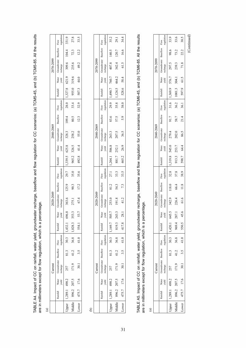
31

TABL

E A4

. Im

pact

of C

C o

n ra

infa

ll, w

ater

yie

ld, g

roun

dwat

er r

echa

rge,

bas

eflo

w a

nd fl

ow r

egul

atio

n fo

r C

C s

cena

rios:

(a)

TC

M5-

45, a

nd (

b) T

CM

5-85

. All

the

resu

lts

are

in m

illim

eter

s ex

cept

for f

low

regu

latio

n, w

hich

is a

per

cent

age.

(a)

C

urre

nt

2020

-204

9 20

40-2

069

2070

-209

9

Rai

nfal

l W

ater

G

roun

dwat

er

Bas

eflo

w

Flow

R

ainf

all

Wat

er

Gro

undw

ater

B

asef

low

Fl

ow

Rai

nfal

l W

ater

G

roun

dwat

er

Bas

eflo

w

Flow

R

ainf

all

Wat

er

Gro

undw

ater

B

asef

low

Fl

ow

yiel

d re

char

ge

re

gula

tion

yi

eld

rech

arge

regu

latio

n

yiel

d re

char

ge

re

gula

tion

yi

eld

rech

arge

regu

latio

n

Upp

er

1,28

9.1

498.

2 25

7 81

.3

30.3

1,

432.

1 69

6.8

363.

6 12

5.9

29.7

1,

339.

5 62

5.8

328.

3 10

9.4

28.0

1,

327.

8 62

1.9

309.

6 10

4.4

331.

9

Mid

dle

896.

2 20

7.5

171.

9 41

.2

36.8

1,

028.

3 35

3.3

275.

1 90

.3

35.0

96

5.2

326.

5 25

8.2

80.5

33

.4

955.

0 31

9.6

235.

6 72

.3

27.8

Low

er

475.

7 17

.6

30.1

3.

5 41

.0

554.

1 53

.7

67.4

17

.2

35.6

49

2.8

41.4

55

.0

12.3

32

.9

507.

3 44

.0

49.2

12

.2

33.5

(b)

C

urre

nt

2020

-204

9 20

40-2

069

2070

-209

9

Rai

nfal

l W

ater

G

roun

dwat

er

Bas

eflo

w

Flow

R

ainf

all

Wat

er

Gro

undw

ater

B

asef

low

Fl

ow

Rai

nfal

l W

ater

G

roun

dwat

er

Bas

eflo

w

Flow

R

ainf

all

Wat

er

Gro

undw

ater

B

asef

low

Fl

ow

yiel

d re

char

ge

re

gula

tion

yi

eld

rech

arge

regu

latio

n

yiel

d re

char

ge

re

gula

tion

yi

eld

rech

arge

regu

latio

n

Upp

er

1,28

9.1

498.

2 25

7 81

.3

30.3

1,

169.

7 50

5.7

253.

0 81

.2

27.1

1,

204.

1 50

6.8

263.

3 83

.6

29.9

1,

490.

7 76

0.7

407.

8 14

0.5

35.2

Mid

dle

896.

2 20

7.5

171.

9 41

.2

36.8

81

9.3

243.

3 19

1.8

54.3

33

.3

881.

7 25

2.1

207.

5 57

.5

35.8

1,

124.

5 46

4.2

342.

4 12

0.7

29.1

Low

er

475.

7 17

.6

30.1

3.

5 41

.0

417.

8 28

.1

41.2

7.

3 33

.5

465.

2 26

.9

36.5

5.

9 38

.0

528.

6 58

.4

61.5

16

.6

34.4

TABL

E A5

. Im

pact

of C

C o

n ra

infa

ll, w

ater

yie

ld, g

roun

dwat

er r

echa

rge,

bas

eflo

w a

nd fl

ow r

egul

atio

n fo

r C

C s

cena

rios:

(a)

TC

M6-

45, a

nd (

b) T

CM

6-85

. All

the

resu

lts

are

in m

illim

eter

s ex

cept

for f

low

regu

latio

n, w

hich

is a

per

cent

age.

(a)

C

urre

nt

2020

-204

9 20

40-2

069

2070

-209

9

Rai

nfal

l W

ater

G

roun

dwat

er

Bas

eflo

w

Flow

R

ainf

all

Wat

er

Gro

undw

ater

B

asef

low

Fl

ow

Rai

nfal

l W

ater

G

roun

dwat

er

Bas

eflo

w

Flow

R

ainf

all

Wat

er

Gro

undw

ater

B

asef

low

Fl

ow

yiel

d re

char

ge

re

gula

tion

yi

eld

rech

arge

regu

latio

n

yiel

d re

char

ge

re

gula

tion

yi

eld

rech

arge

regu

latio

n

Upp

er

1,28

9.1

498.

2 25

7 81

.3

30.3

1,

420.

1 64

5.5

342.

9 11

8.0

32.8

1,

319.

8 54

5.0

279.

4 91

.7

31.6

1,

369.

9 57

6.7

297.

5 98

.6

33.9

Mid

dle

896.

2 20

7.5

171.

9 41

.2

36.8

96

9.4

287.

1 22

6.4

66.4

37

.8

913.

3 25

3.7

202.

0 58

.7

36.2

10

01.3

30

4.1

239.

3 73

.2

33.6

Low

er

475.

7 17

.6

30.1

3.

5 41

.0

550.

5 45

.6

61.6

11

.8

38.9

59

8.7

64.4

86

.5

21.4

36

.1

597.

9 61

.5

71.8

22

.2

38.5

(Con

tinued)

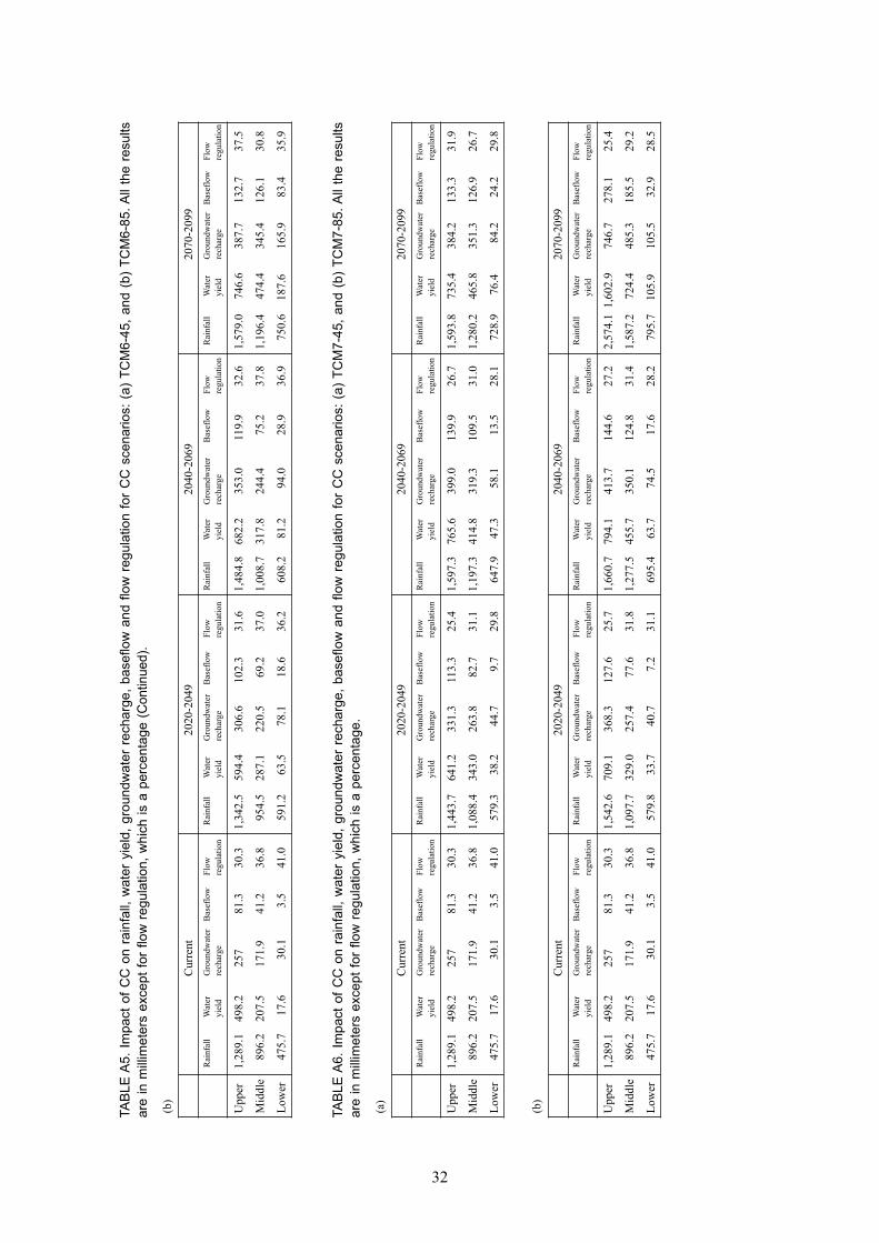
32

TABL

E A5

. Im

pact

of C

C o

n ra

infa

ll, w

ater

yie

ld, g

roun

dwat

er r

echa

rge,

bas

eflo

w a

nd fl

ow r

egul

atio

n fo

r C

C s

cena

rios:

(a)

TC

M6-

45, a

nd (

b) T

CM

6-85

. All

the

resu

lts

are

in m

illim

eter

s ex

cept

for f

low

regu

latio

n, w

hich

is a

per

cent

age

(Con

tinue

d).

(b)

C

urre

nt

2020

-204

9 20

40-2

069

2070

-209

9

Rai

nfal

l W

ater

G

roun

dwat

er

Bas

eflo

w

Flow

R

ainf

all

Wat

er

Gro

undw

ater

B

asef

low

Fl

ow

Rai

nfal

l W

ater

G

roun

dwat

er

Bas

eflo

w

Flow

R

ainf

all

Wat

er

Gro

undw

ater

B

asef

low

Fl

ow

yiel

d re

char

ge

re

gula

tion

yi

eld

rech

arge

regu

latio

n

yiel

d re

char

ge

re

gula

tion

yi

eld

rech

arge

regu

latio

n

Upp

er

1,28

9.1

498.

2 25

7 81

.3

30.3

1,

342.

5 59

4.4

306.

6 10

2.3

31.6

1,

484.

8 68

2.2

353.

0 11

9.9

32.6

1,

579.

0 74

6.6

387.

7 13

2.7

37.5

Mid

dle

896.

2 20

7.5

171.

9 41

.2

36.8

95

4.5

287.

1 22

0.5

69.2

37

.0

1,00

8.7

317.

8 24

4.4

75.2

37

.8

1,19

6.4

474.

4 34

5.4

126.

1 30

.8

Low

er

475.

7 17

.6

30.1

3.

5 41

.0

591.

2 63

.5

78.1

18

.6

36.2

60

8.2

81.2

94

.0

28.9

36

.9

750.

6 18

7.6

165.

9 83

.4

35.9

TABL

E A6

. Im

pact

of C

C o

n ra

infa

ll, w

ater

yie

ld, g

roun

dwat

er r

echa

rge,

bas

eflo

w a

nd fl

ow r

egul

atio

n fo

r C

C s

cena

rios:

(a)

TC

M7-

45, a

nd (

b) T

CM

7-85

. All

the

resu

lts

are

in m

illim

eter

s ex

cept

for f

low

regu

latio

n, w

hich

is a

per

cent

age.

(a)

C

urre

nt

2020

-204

9 20

40-2

069

2070

-209

9

Rai

nfal

l W

ater

G

roun

dwat

er

Bas

eflo

w

Flow

R

ainf

all

Wat

er

Gro

undw

ater

B

asef

low

Fl

ow

Rai

nfal

l W

ater

G

roun

dwat

er

Bas

eflo

w

Flow

R

ainf

all

Wat

er

Gro

undw

ater

B

asef

low

Fl

ow

yiel

d re

char

ge

re

gula

tion

yi

eld

rech

arge

regu

latio

n

yiel

d re

char

ge

re

gula

tion

yi

eld

rech

arge

regu

latio

n

Upp

er

1,28

9.1

498.

2 25

7 81

.3

30.3

1,

443.

7 64

1.2

331.

3 11

3.3

25.4

1,

597.

3 76

5.6

399.

0 13

9.9

26.7

1,

593.

8 73

5.4

384.

2 13

3.3

31.9

Mid

dle

896.

2 20

7.5

171.

9 41

.2

36.8

1,

088.

4 34

3.0

263.

8 82

.7

31.1

1,

197.

3 41

4.8

319.

3 10

9.5

31.0

1,

280.

2 46

5.8

351.

3 12

6.9

26.7

Low

er

475.

7 17

.6

30.1

3.

5 41

.0

579.

3 38

.2

44.7

9.

7 29

.8

647.

9 47

.3

58.1

13

.5

28.1

72

8.9

76.4

84

.2

24.2

29

.8

(b)

C

urre

nt

2020

-204

9 20

40-2

069

2070

-209

9

Rai

nfal

l W

ater

G

roun

dwat

er

Bas

eflo

w

Flow

R

ainf

all

Wat

er

Gro

undw

ater

B

asef

low

Fl

ow

Rai

nfal

l W

ater

G

roun

dwat

er

Bas

eflo

w

Flow

R

ainf

all

Wat

er

Gro

undw

ater

B

asef

low

Fl

ow

yiel

d re

char

ge

re

gula

tion

yi

eld

rech

arge

regu

latio

n

yiel

d re

char

ge

re

gula

tion

yi

eld

rech

arge

regu

latio

n

Upp

er

1,28

9.1

498.

2 25

7 81

.3

30.3

1,

542.

6 70

9.1

368.

3 12

7.6

25.7

1,

660.

7 79

4.1

413.

7 14

4.6

27.2

2,

574.

1 1,

602.

9 74

6.7

278.

1 25

.4

Mid

dle

896.

2 20

7.5

171.

9 41

.2

36.8

1,

097.

7 32

9.0

257.

4 77

.6

31.8

1,

277.

5 45

5.7

350.

1 12

4.8

31.4

1,

587.

2 72

4.4

485.

3 18

5.5

29.2

Low

er

475.

7 17

.6

30.1

3.

5 41

.0

579.

8 33

.7

40.7

7.

2 31

.1

695.

4 63

.7

74.5

17

.6

28.2

79

5.7

105.

9 10

5.5

32.9

28

.5

IWMI Working Papers

178 Understanding the Hydrological Impacts of Climate Change in the Tana River Basin, Kenya. Aditya Sood, Lal Muthuwatta, Nishchitha Sandeepana Silva and Matthew McCartney. 2017.

177 Sticks and Carrots: Managing Groundwater Over-abstraction in La Mancha, Spain. Alvar Closas, François Molle and Nuria Hernández-Mora. 2017.

176 Adapting Aquifer Storage and Recovery Technology to the Flood-prone Areas of Northern Ghana for Dry-season Irrigation. Seth Owusu, Olufunke O. Cofie, Paa Kofi Osei-Owusu, Vincent Awotwe-Pratt and Marloes L. Mul. 2017.

175 Public Participation in Environmental Impact Assessment of Hydropower Plants in Nepal: A Context-specific Approach. Jon Munch-Petersen. 2017.

174 Smallholder Irrigation Schemes in the Limpopo Province, South Africa. Barbara van Koppen, Luxon Nhamo, Xueliang Cai, Mary Jean Gabriel, Mosibudi Sekgala, Sydney Shikwambana, Khathu Tshikolomo, Shalon Nevhutanda, Boshomane Matlala and David Manyama. 2017.

173 Agro-climatic and Hydrological Characterization of Selected Watersheds in Northern Ghana. Davie M. Kadyampakeni, Marloes L. Mul, Emmanuel Obuobie, Richard Appoh, Afua Owusu, Benjamin Ghansah, Enoch Boakye-Acheampong and Jennie Barron. 2017.

172 Mapping Irrigated Areas in the Limpopo Province, South Africa. Xueliang Cai, James Magidi, Luxon Nhamo and Barbara van Koppen. 2017.

171 Multiple Uses of Small Reservoirs in Crop-livestock Agro-ecosystems of the Volta River Basin with an Emphasis on Livestock Management. Augustine. A. Ayantunde, Mawa Karambiri, Viviane Yameogo and Olufunke O. Cofie. 2016.

170 An Assessment of Integrated Watershed Management in Ethiopia. Gebrehaweria Gebregziabher, Dereje Assefa Abera, Girmay Gebresamuel, Meredith Giordano and Simon Langan. 2016.

169 Methods to Investigate the Hydrology of the Himalayan Springs: A Review. Pennan Chinnasamy and Sanmugam A. Prathapar. 2016.

168 Measuring Transboundary Water Cooperation: Learning from the Past to Inform the Sustainable Development Goals. Davison Saruchera and Jonathan Lautze. 2015.

IWMI provides free access to all its publications.Visit

www.iwmi.org/publications/index.aspx

ISSN: 2012-5763e-ISSN: 2478-1134ISBN: 978-92-9090-860-9

Postal AddressP O Box 2075ColomboSri Lanka

Location127 Sunil MawathaPelawattaBattaramullaSri Lanka

Telephone+94-11-2880000

Fax+94-11-2786854

[email protected]

Websitewww.iwmi.org

Documents

Understanding the hydrological impacts of climate change