Embed Size (px)
Citation preview

1
“Understanding the Effects of Violent Video Games on Violent Crime”
A. Scott Cunningham, Baylor University
Benjamin Engelstätter, ZEW Mannheim
Michael R. Ward, University of Texas at Arlington
April, 2011
ABSTRACT: Psychological studies invariably find a positive relationship between violent video game play and aggression. However, these studies cannot account for either aggressive effects of alternative activities video game playing substitutes for or the possible selection of relatively violent people into playing violent video games. That is, they lack external validity. We investigate the relationship between the prevalence of violent video games and violent crimes. Our results are consistent with two opposing effects. First, they support the behavioral effects as in the psychological studies. Second, they suggest a larger voluntary incapacitation effect in which playing either violent or non-violent games decrease crimes. Overall, violent video games lead to decreases in violent crime.
JEL Codes: D08, K14, L86
Keywords: Video Games, Violence, Crime

2
“Understanding the Effects of Violent Video Games on Violent Crime”
1. Introduction
From the sensational crime stories of the 19th
century (Comstock and Buckly 1883), to
the garish comic books of the early 20th
century, (Hadju 2009), to today‟s violent video
games, Americans have made efforts to reduce children‟s access to violent media because of
concerns over their social costs. These concerns may not be unfounded as numerous studies
purport to find that violent media of all sorts, including games, can cause increases in
measured aggression. Aided in part by mounting evidence that violent video game play cause
aggression, states have passed legislation criminalizing the distribution of violent video games
to minors.1
The research is not clear on how large the increase in aggression caused by these
games. Craig Anderson, a long-time researcher in the effect of violent media on aggression
has contended that "one possible contributing factor [to the Columbine High School killings
was the shooters‟ habits of playing] violent video games. [The shooters] enjoyed playing the
bloody shoot-`em-up video game Doom, a game licensed by the U.S. Army to train soldiers to
effectively kill" (quoted in Kutner and Olson 2009).2
If violent video games can be shown to cause violence, then laws aimed at reducing
access may benefit society at large. Yet to date, though there is ample evidence that violent
video games cause aggression in a laboratory setting, laboratory stings cannot address
selection or incapacitation. Ward (2010) shows that adolescents who are otherwise
predisposed to violence tend to select into video game play. Likewise, since the hours it takes
to "beat the game" substitute for some other activity, a complete analysis must consider the
1 In 2010, California passed a law making it a punishable offense for a distributor to sell a banned violent video
to a minor. The case is currently before the US Supreme Court. 2 In the opening paragraph of his literature review, Anderson (2004) suggested violent video games were
responsible for the recent wave of school shootings since the late 1990s.

3
opportunity cost of this time. Violence may fall because gamers engaged in virtual violence
are not simultaneously engaged in actual violence.
To date, there is no evidence that violent video games cause violence or crime. In fact,
two recently published studies analyzed the effect of violent media (movies and video game
stores) on crime, and found increased exposure may have caused crime rates to decrease
(Dahl and Dellavegna 2009; Ward 2011). These studies, unlike the laboratory studies, were
conducted with observational data, which poses unique scientific challenge to establishing
causality. However, since laboratory studies have never shown that video game violence
causes crime or violence, despite researchers out-of-sample predictions (Anderson 2004),
observational studies may be the only ethical and practical way to test for such a causal effect.
To many in this field, it is logical to assume that if exposure to violent media causes
aggression in the lab, that it will therefore cause aggression when exposure occurs non-
randomly outside the laboratory, including other outcomes associated with aggression, such as
crime and violence. In this paper, we argue that since laboratory experiments have not
examined the time use effects of video games, which incapacitate violent activity by drawing
individual gamers into extended gameplay, laboratory studies may be poor predictors of the
net effects of violent video games in society. Consequently, they overstate the importance of
video game induced aggression as a social cost. We argue that since both aggression and time
use are a consequence of playing violent video games, then the policy relevance of violent
video game regulation depends critically on the degree to which the one outweighs the other.
If, as we find in our study, the time use effect of violent video games reduce crime by more
than the aggression effects increase it, then the case for regulatory intervention becomes
weaker. While some early work has been done on the long-term effects of video game play,

4
nearly all the laboratory evidence that currently exists has only uncovered very short-term
effects, which is when time use effects could be the most important.3
As with Dahl and Dellavegna (2009) and Ward (2011), we use a proxy for individuals‟
exposure to violent video games – the volume of sales of violent video games in a week
among the top 50 best-selling video games from 2005-2008 – and relate it to a marker for
violent behaviors – weekly aggregate violent crime incidents from the National Incident
Based Reporting System (NIBRS). Using time series modeling, as well as an instrumental
variables approach, we estimate the effect of an increased volume of violent video game sales
over the period on the number of criminal incidents recorded to law enforcement at the
weekly level and find that increased violent video games are associated with decreases in
crime rates, similar to Dahl and Dellavegna (2009) and Ward (2011).
One advantage of our approach is that we can attempt to disentangle the separate
effects of both a behavioral change toward more aggression and incapacitation due to time
use. Our results provide some support for the psychological finding that, absent
incapacitation, violent video games lead to more violent crimes. However, our results also
indicate this is dominated by an incapacitation effect leading to a net reduction in violent
crimes. This approach can help guide investigators into the design of more holistic research
designs, such as field experimentation and other quasi-experimental methodologies, to
determine whether the net social costs of violent games are non-trivial. The shortcoming of
our approach is due to the limitations of our data on game sales. Unfortunately, the industry
does not report cross-sectional variation in game sales – only the national weekly sales of the
top 50 highest grossing games are available. As a result, our paper follows a methodology
3 In Anderson (2004), the author notes the glaring omission of longitudinal studies of effects of violent video
games on aggression in his conclusions on the state of the research, calling for more studies aimed at
investigating the long-term effects. If nothing else, though, this makes our point that the abundance of evidence
that we know does exist only speaks to short-term effects of violent video games on aggression, which is the
purpose of this study here.

5
similar to Dahl and Dellavegna (2009), who estimated the impact of violent movies, proxied
by daily ticket sales, on crime using only time series methods.
The paper is structured as follows: the second section presents our theoretical
modeling of the effect of violent video games on crime based on the general aggression model
(GAM) using Becker and Murphy‟s theory of addiction and Becker‟s theory time use. The
third section presents our data and methodology. The forth presents and discusses our results.
We conclude with a brief discussion of the implications for public policy.
II. Theory of Violent Video Games Effect on Crime
To make the theoretical concerns more transparent, we present versions of both the
leading psychological theory of violent video games‟ effect on aggression, as well as
canonical economic models that can incorporate psychological insights, to illustrate how
violent video game play can have ambiguous effects on crime and severe aggression despite a
positive effect on the aggressive tendencies of a person. We modify the Becker and Murphy
(1988) addition model to a video game setting to get a version of a general aggression model
(GAM). At the same time, a common observation is that new releases of popular video games
often results in long hours of play by gamers. We apply the time allocation model of Becker
(1965) to the video game setting to show that the resultant „voluntary incapacitation‟ could
reduce violent outcomes.
A. Incorporating GAM into a Rational Addiction Model
Though the empirical foundation of a causal effect of violent video games on
aggression has been carefully documented in decades of experimental work, social-
psychological theories explaining this empirical relationship is relatively new. Bushman and
Anderson (2002) and Anderson and Bushman (2002) present a psychological theory of such a
link that they call the general aggression model, or GAM. GAM hypothesizes that violent

6
media, including violent video games, increases a person‟s aggressive tendencies through a
process of social learning that occurs simultaneous to the exposure itself. Violent media
causes the person to mistakenly develop certain scripts, or rules of thumb, that are used to
interpret social situations both before they occur, as well as afterwards. GAM posits, in other
words, that violent video games cause aggression by biasing individuals towards forming
incorrect beliefs about relative danger that they are in. Perception biases towards hostility,
therefore, can in turn cause the person to respond in either a “fight or flight” fashion. It may
also permanently alter a person‟s point of view, creating an aggressive personality as an
outcome (Bushman and Anderson 2002).
The GAM is, in many ways, a description of a person‟s own production function in
which time inputs are mixed with virtual media to produce thoughts and sensations. The
accidental byproduct of this production, though, is that the exposure may also modify the
person‟s future capital stock for producing aggression such that current consumption can
change the future productivity of aggression.
The “rational addiction” model (Becker and Murphy 1988) encompasses behaviors
that may not meet a psychological definition of addiction. The key insight for GAM is that
consumption of a good in one period not only affects current utility directly and, through a
capital stock accumulation mechanism, but also affects future utility indirectly. For example,
drinking alcohol today builds up one‟s tolerance for alcohol (desensitization) that is modeled
as a stock variable that increases the marginal utility. Hence, current consumption increases
the agent‟s optimal level of future alcohol consumption. In our context, we do not model
video game play as addictive itself, but rather we consider that violent video game play could
affect future utility from aggressive behaviors.
The model primitives include per period utility:
7
( )
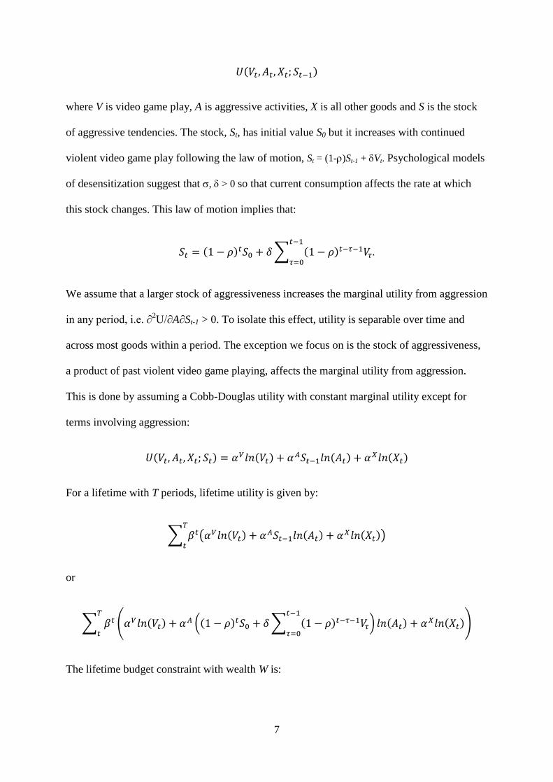
where V is video game play, A is aggressive activities, X is all other goods and S is the stock
of aggressive tendencies. The stock, St, has initial value S0 but it increases with continued
violent video game play following the law of motion, St = (1-)St-1 + Vt. Psychological models
of desensitization suggest that , > 0 so that current consumption affects the rate at which
this stock changes. This law of motion implies that:
( ) ∑ ( )
We assume that a larger stock of aggressiveness increases the marginal utility from aggression
in any period, i.e. ∂2U/∂A∂St-1 > 0. To isolate this effect, utility is separable over time and
across most goods within a period. The exception we focus on is the stock of aggressiveness,
a product of past violent video game playing, affects the marginal utility from aggression.
This is done by assuming a Cobb-Douglas utility with constant marginal utility except for
terms involving aggression:
( ) ( )
( ) ( )
For a lifetime with T periods, lifetime utility is given by:
∑ ( ( ) ( )
( ))
or
∑ ( ( ) (( ) ∑ ( )
) ( )
( ))
The lifetime budget constraint with wealth W is:

8
∑ (
)
Consistent with Becker and Murphy (1988), consumers are forward looking as to the
effect of video games on future aggression. Let be the Lagrange multiplier on the wealth
constraint. They maximize lifetime utility with respect to video game play and aggression in
each period subject to their wealth constraint. This yields 3T first-order conditions and 3T
unknowns. The first-order condition for video game play in period t is:
∑ ( ) ( )
The first term on the left represents the direct effect of video game play on current period
utility while the second represents an indirect effect of current video game play on utility in
all subsequent periods through its effect on the marginal utility from aggression. Agents
consider both effects when they respond to an exogenous shock to video game prices. All else
equal, a relatively lower current price of video games will imply relatively more current
period video game play. In the empirical model below, we identify a price reduction with an
exogenous increase in the quality of games.
The first-order condition for aggression in period t is:
(( ) ∑ ( )
)
This implies that agents choose to be more aggressive when their current stocks of aggressive
tendencies are higher. These stocks will be higher if they have recently consumed relatively
more video games because of relatively lower recent video game prices (or higher video game
quality). Thus, the dynamics are as follows. Even forward looking agents respond to
temporarily low video game prices with temporarily more video game play. This results in a

9
temporary increase in the stock of aggressive tendencies in subsequent periods and, thus, a
temporary increase in aggressive behaviors in subsequent periods.
While the model predicts specific inter-temporal linkages, it is silent on how long the
time horizon would be for an aggressive response to an exogenous increase in video game
play. Depending on how fast the stock parameter depreciates, the value of , it might be that
the aggression rises and falls over days, weeks or even years. To date the psychological
literature studying the impact of violent video games on aggression has focused primarily on
short-run, intra-day, responses as opposed to longitudinal outcomes (Anderson 2004). In our
empirical analysis below, we can only test over a few weeks‟ time. However, we note that we
are unaware of any empirical studies linking media violence to aggressive behavior more than
a few weeks later.4
B. Incorporating Violent Video Game Effects into a Time Use Model
The opportunity cost of playing a video game is not just pecuniary but also includes
lost time. In fact, for many gamers, the value of the time spent playing a game may be worth
much more than the pecuniary cost of the game. This time spent gaming cannot be spent on
other activities, both legitimate activities and illicit violent activities, if time use is rival in
consumption. Evidence for video game having a time use component can be found in
Stinebrickner and Stinebrickner (2008). The authors identified a causal effect of studying on
academic performance by utilizing the random assignment of college students to roommates
with a video game console, relative to the counterfactual, which caused students to study less
often, and in turn, to perform worse in school.
Even if a gamer is predisposed to being more aggressive due to gaming, he can
express this aggression only over a shorter time non-gaming period. In contrast to the
4 Ward (2011) does relate yearly variation in video game demand to annual changes in crimes and deaths.

10
heightened aggressive tendencies described in our modified GAM-addiction model,
„voluntary incapacitation‟ of the gamer while gaming would tend to reduce aggressive
outcomes, without necessarily a reduction in long-term aggressive tendencies.
To see this, we develop a simple model of time allocation (Becker (1965). Consider a
single period model in which agents get utility from playing video games, from acts of
aggression, and from all other goods, U(V, A, X). Consumption of one unit of any good
involves both pecuniary and time costs. For simplicity assume a linear consumption
technology in which consumption of one unit of good i entails a pecuniary price pi and a time
cost ri. In addition, the agent can convert time into income by working h hours at wage w.
Now agents face two constraints:
These two conditions can be combined through h to yield:
( ) ( ) ( )
Let be the Lagrange multiplier for this constraint. Optimality is determined from the first-
order conditions for utility maximization:
( )
( )
( )
( )
( )
( )
For standard utility functions, these four equations and four unknowns yield a unique interior
solution. One implication is that consumption of a good depends on the „full‟ price i.e., video
game demand depends on pV + wrV. A reduction in the pecuniary price of video games, pV,
will lead to an increase in consumption of video games. However, this increase in video game

11
play entails both pecuniary and time costs. It could be that video game play does not affect the
marginal utility from aggression, or indeed it may augment it, i.e., ∂2U/∂A∂X > 0. However, if
the ratio time costs to pecuniary costs of video games, rV/pV ,is relatively large, the consumer
will tend to substitute away from other activities with relatively high time to pecuniary cost
ratios. Committing acts of aggression tend to fit this description.
III. Data and Methodology
Randomized assignment of a treatment with comparison groups used to make
comparative counterfactuals is widely considered the “gold standard” in the social sciences
(Fisher 1935; Campbell and Stanley 1963; Rosenbaum 2002). Yet, it is widely known that
experimentalism may fail to identify true causal effects for a variety of reasons (Berk 2005;
Deaton, 2010; Heckman and Urzua, 2010; Imbens 2010). While others have noted the failure
of researchers in this literature to satisfy the rigorous conditions for establishing causality
(Ferguson and Kilburn 2008; Olson and Kuttner 2009) our article will focus on a separate
statistical challenge not mentioned in these earlier studies: the challenge of internal versus
external validity.
Finding of a positive effect of violent games on aggression does not therefore mean
that violent video games played will cause crime if the incapacitation effects from time use
swamp the marginal increase in aggression in the person. By design, laboratory studies – both
by ignoring alternative time use and by treating both treatment and control groups with this
separate effect – cannot be used to guide researchers as to what expect outside the lab. In this
sense, the studies have internal, but may not have external validity on the incidence of
socially costly aggression from violent video game play (Campbell and Stanley 1963). Quasi-

12
experimental methods, such as panel econometric methods, regression discontinuity and
instrumental variables, as well as field experimentation (Harrison and List 2004; Angrist
2006) may be more suitable estimating the social costs of violent video games since they
allow for the estimation of all known and unknown theoretical mechanisms. In this section,
we explain our research design and the data used to overcome some of the limitations of a
purely experimental methodology.
A. Empirical Methodology
These models of video game violence suggest that the effect of violent video game play
on crime will depend on whether a sizable stock of aggressive tendencies accumulates and on
the games‟ time use intensities. On the one hand, violent games that raised the players‟ stock
of aggression would cause crime rates to be increasing in the amount of violent video games
played, depending on the rate at which that stock eroded during nonuse. But because games
can be thought of as a kind of entertainment commodity that the agent consumes through time
usage, even violent games might decrease crime if voluntary incapacitation due to game play
crowds out time spent engaging in activities that lead to criminal acts.
Given that the theoretical predictions are ambiguous, the policy relevance of the
laboratory studies is unclear, suggesting that more empirical work outside of a laboratory
context is warranted. However, without experimental data, causal inference is problematic.
Correlations between video game play and crime may or may not reflect a causal relationship
if the unobserved determinants of crime are correlated with video game play. For instance,
bad weather such as rain or heavy snow which causes individuals to remain at home would
both increase the likelihood of playing video games and decrease the returns to crime through

13
higher chances of finding a resident at home.5 Hence, negative correlations between crime and
violent video game play could purely be a consequence of omitted variable bias.
One solution to omitted variable bias when there is time-variant heterogeneity is to
employ instrumental variables (IVs) assuming the researcher has an instrument that is
strongly correlated with individual game play but uncorrelated with the determinants of crime.
This approach exploits exogenous variation in video game play that is not due merely to
changes in the determinants of crime providing greater assurance that the estimated effect is
causal. We use the ratings of video games by a video games rating agency as IVs. Our IV
strategy exploits the variation in game sales correlated only with the variation in quality, and
thus is mostly free of variation due to factors related to crime.
Zhu and Zhang (2010) show that consumer reviews of video games are positively
related to game sales. Ratings are valuable pieces of information for video games because
games are complex experience goods for which gamers cannot know their preferences
without playing. Our data on professional ratings contain rich information that communicates
the kinds of information that gamers value in forecasting their beliefs about the game, and as
beliefs and anticipation are drivers of the game sales, we would expect these rating
institutions to play important roles in forming consumer prior beliefs about the game and
therefore their purchases. But we also have some evidence from other industries that would
suggest scores would independently cause purchases to rise, independent of the unobserved
factors that cause expert opinion and purchases to be highly correlated. Reinstein and Snyder
(2005) used exogenous variation in Siskel and Ebert ratings due to disruptions in their pair‟s
reviewing to determine a causal effect on movie demand. More recently, Hilger Rafert and
Villas-Boas (2010) found that randomly assigned expert scores on bottles of wine in a retail
5 While the example is a valid concern for measures of video game play, it may be less problematic for this study
given that we do not use high frequency game play as a measure of violent video game consumption. Rather, we
use sales in a week, which mitigates some of the concerns over weather given that it is the cumulative sales of
games that determines our measure of consumption, which should be relatively insensitive to changing weather
conditions on a given day.

14
grocery store caused an increase in sales for the higher rated, but less expensive, wines. While
these studies do not confirm that there are exogenous forces in video game ratings that drive
consumer purchases, they are suggestive.
We begin by estimating a standard multivariate regression model of the incidence of
various crimes as functions of, among other controls, the prevalence of non-violent and
violent video games. Our outcome variable of interest, Ct,, is the number of new and reported
criminal incidents in week t. While the dataset we use documents criminal offenses on a daily
basis, since the video game sales data are available only on a weekly basis, we aggregate
crimes into weekly measures to focus on same-week exposure. Accordingly, we employ a
simple least squares estimator so as to more easily instrument for video game exposure.6
Our main explanatory variables are aggregated current and lagged values of weekly
sales volumes for both non-violent and violent video games. Video games appear to
depreciate quickly. This may be because new games are played intensively for a few weeks
after purchase and are not replaced with a new game until after some diminishing returns have
been reached, or it may suggest that firms typically stagger the release dates of games. We
measure the cumulative effect of games with the sales volume of the current week‟s sales
along with the various lags of previous weeks‟ sales so as to capture the effect of higher
volume of gameplay with unknown time to triggered crime. Following the models developed
in section 2 the benchmark specification is:
( ) ( ) (
)
The number of crime incidents depends on the exposure to intensive violent video games
and not intensively violent games
. The coefficient can be interpreted as the
percent increase in crime incidents for each percent increase in intensively violent video
games sold in week t. can be interpreted accordingly covering the impact of not
6 Our empirical methodology is in large part based on Dellavegna and Dahl‟s (2008) study of the effect of movie
violence on crime.

15
intensively violent video games. The identification of the parameters is based on the time-
series variation in the style of violence in the video games. Comparing the estimates of
and a difference-in-difference estimate of the effect of intensely violent video games
versus not intensely violent games can be achieved. The benchmark specification contains
additionally seasonal controls in form of dummy variables for months and a time trend to
account for a general decline in crimes over time.
The measured effect from this specification can represent a confluence of many
effects. It is possible for there to be a positive behavioral effect, as found in the laboratory,
and a negative voluntary incapacitation effect. This specification could only measure the net
effect. It may be possible to disentangle the behavioral effects from the incapacitation effect
by addressing whether the mix of crimes becomes more or less violent as a result of violent
video game exposure. Using the FBI‟s classification of crimes as violent or non-violent, we
estimate:
( ) ( ) (
)
where VCt is the number of violent crimes. This specification measures whether violent and
non-violent video game play has a larger effect on violent or non-violent crimes. A positive
estimated value of would indicate that the violent video games have a positive effect on
violent crimes relative to all crimes. Under the assumption that incapacitation results equally
for violent and non-violent crimes, this would indicate that violent video games induce
behaviors toward violent crimes.
Besides the benchmark specification we employ two additional specifications as
robustness checks. The specifications cover specific segments of the population we expect to
be more frequent gamers, e.g. people aged between 15 and 30 years and high school and
college students. For each crime incident, NIRBS provides information on the age of the
offender and on the location of the incident. In the first robustness check, we select our
sample for offenders aged between 15 and 30 years and compare these results to the results

16
obtained from the sample of offenders who are 35 to 50 years old. In our second check, we
extend our estimation procedure to compare the effects on the number of incidents reported
on school campuses to the number committed at other locations.
B. Video Game Sales Data
Our treatment variables for video game play are derived from video game unit sales
volume data from VGChartz7. Beginning consistently in 2005, this site has provided unit sales
volume information for each of the top 50 selling video console games each week. Sales
volumes are reported for several geographical areas including worldwide reports and amounts
for specific countries like USA, Japan, Europe, Middle East, Africa or Asia. In addition,
VGChartz provides information about the publisher and the console for each game. In our
sample period 2005 to 2008 the VGChartz dataset contains 1,091 different titles over the 208
weeks for the US with some of these titles being the same game for different gaming
consoles. In sum, the games are provided from 47 different publishers and designed for nine
different gaming consoles. While VGChartz includes the top 50 selling games each week, it
only covers a portion of all sales in the US video game market. A game‟s week of release is
almost always its top selling week. Figure 1 indicates that most games stay in the top 50 for
only a few weeks. Moreover, as Figure 2 indicates, the top selling games sell much more than
even the lower ranked top 50 games. These features suggest that there is considerable week-
to-week variation in the games, and the types of games, being played. According to the
Entertainment Software Association (ESA)8 VGChartz account for about one-quarter of the
2005 units (ESA Annual Report, 2010). This fraction rises to almost one-half in 2008.
Our measure of violent videogame content stems from the Entertainment Software
Rating Board (ESRB).9 This non-profit body independently assigns a technical rating (E, E10,
T, M, and A) which defines the audience the game is appropriate for where E classifies games
7 http://www.vgchartz.com/
8 http://www.theesa.com – The reported numbers from ESA also include games for personal computers which
amount to about 10 percent of the market each year and are intentionally not included in VGChartz. 9 http://www.esrb.org

17
for everybody, E10 for everyone aged 10 and up, T for teens, M games for a mature audience,
and A for adult content. In addition, ESRB provides detailed description of the content in each
game on which the rating was made, including the style of violence, e. g. language, violence,
or adult themes. For all of the 1,091 titles in our sample we collected the appropriate ESRB-
rating and all content descriptors. Based on this content information we identify 762 non-
violent and 329 violent games, of which 105 titles are described as intensely violent. Almost
all violent games are mostly rated T or M. All intensely violent games are rated M. Merging
both data sources together we can construct measures of the aggregate unit sales of non-
violent, violent, and intensely violent video games for each week. The weekly sales are
pictured in Figure 3 for all games and intensely violent games. Overall, the two graphs follow
a similar pattern with a peak around the Christmas gift purchasing period. In the mid of 2008,
however, the intense violent games seem to account for almost all sales of the violent games.
As argued in section 2, the prevalence of video games in a week is not randomly
distributed over the sample and therefore may be endogenous. For instance, if changing
economic conditions caused unemployment to rise, and in turn crime rates, as well as caused
leisure activities like video games to rise, then we might observe positive correlations
between video game play and crime that is driven purely by these changing economic factors
(Raphael and Winter-Ebmer 2001; Gould, Weinberg and Mustard 2002). We address the
potential endogeneity of video games with instrumental variables using expert review of each
title as an instrument for purchases.
Our expert review data comes from the GameSpot website.10
GameSpot provides
news, reviews, previews, downloads and other information for video games. Launched in
May 1996 GameSpot‟s main page has links to the latest news, reviews, previews and portals
for all current platforms. It also includes a list of the most popular games on the site and a
search engine for users to track down games of interest. The GameSpot staff reviewed almost
10
http://www.gamespot.com

18
every game in our sample and rated the quality of the titles on a scale from 1 to 10 with 10
being the best possible rank. These so called GameSpot-scores assigned to each game are
intended to provide an at-a-glance sense of the overall quality of the game. The overall rating
we employ is based on evaluations of graphics, sound, gameplay, replay value and reviewer‟s
tilt. A possible issue with this measure is that GameSpot changed the rating system in mid of
2007 to employ guidelines and a philosophy focusing more on a prospective customer rather
than a hardcore-fan that the reviewers had focused on before. Nevertheless, the five
mentioned aspects are essential parts of a game that are still reviewed in detail by a GameSpot
reviewer but will not get an own rating score anymore. We do not consider this change in the
GameSpot focus to noticeably affect the overall GameSpot-score.
We expect the quality rating of the games to be positively correlated with their sales as
better-rated games usually are more highly demanded. It is possible that some games have the
opposite relationship if they are based on a popular tie-in from a movie, e. g. Harry Potter, or
sequels, e. g. the Final Fantasy series. Developers know that these games will sell well due to
their popular tie-in which may lower the returns to investment in game quality. However, in
table 2 we show that, a game title‟s weekly sales are positively related to the Game Spot score
for games of different violence profiles.
C. Crime Data
For our measure of weekly crime, we used the National Incident Based Reporting
System, or NIBRS. NIBRS is a federal data collection program begun by the Bureau of
Justice Statistics in 1991 for gathering and distributing detailed information on criminal
incidents for participating jurisdictions and agencies. Participating agencies and states submit
detailed information about criminal incidents not contained in other data sets, such as the
Uniform Crime Reports. For instance, whereas the Uniform Crime Reports contain
information on all arrests and cleared offenses for the eight Index crimes, NIBRS consists of
individual incident records for all eight index crimes and the 38 other offenses (Part II

19
offenses) at the calendar date and hourly level (Rantala and Edwards 2001). Because of the
detailed information about the incident, including the precise time and date of the incident,
economists such as Dahl and Dellavegna (2009), Card and Dahl (2009), Jacob and Moretti
(2003) and Lefgren, Jacobs and Moretti (2007) have used it for event studies. In our case, we
exploit detailed information about the age of offenders and the crime‟s location – on school
campuses or not – for our robustness checks.
Crimes follow a seasonal pattern. Figure 4 indicates a consistent pattern of gradual
increases in both violent and non-violent crimes from winter to summer. Our method was
developed to account for seasonality in both of our main variables of interest crime and
games. Much of the seasonality in crimes is believed to be due to weather while seasonality in
games is likely due to holiday gift giving (Lefgren, Jacobs and Moretti 2007). Failure to
address this will likely lead to spurious correlations. As indicated above, we accommodate
this in two ways. First, month dummy variables should capture much of the seasonality.
Second, using Game Spot scores as IVs should isolate the variation in game sales due to game
quality.
Our final sample includes 208 weekly observations on video games sales and crimes
from early 2005 through 2008. However, eight observations are excluded from final
regressions because of the use of lagged video game sales. Table 3 reports basic descriptive
statistics for our sample.
IV. Results
A. Basic Results
Our basic regression results are presented in Tables 4 and 5. Table 4 reports estimates
of various specifications of the effect video games sales on all crimes from equation (1)
above. Video games are separated between those that the ESRB rated as “intensely violent”

20
and those that are not. Recall that the lesser rating of merely “violent” does not warrant an
ESRB rating of “M.”11
Control variables include month dummies to capture seasonality and a
time trend to capture any secular trend. The columns from left to right add more lags of video
games to the specification so as to measure possible inter-temporal effects of game purchase
in one week affecting crime in subsequent weeks through continued play. Finally, each
regression employs a 2SLS estimator with the same set of current and eight lags of Game
Spot scores averaged over intensely violent games and over games that are not intensely
violent. Since the specifications are over-identified, we test for possible endogeneity of the
instrument set. As expected, in all cases, we fail to reject the exogeneity of Game Spot scores
with respect to the level of crime.
The estimated effect of video games sales in any single week is small. Most individual
coefficient estimates are negative but few are significantly different from zero. It appears that
lags of up to five weeks of video game sales may be associated with current crime. It is not
clear from this table whether violent games have a different effect from those that are not
violent. For ease of comparison, we report the sum of the coefficients for various lags for both
in the top panel of Table 6 to calculate the cumulative effect of a change in video games over
time. Here it becomes clear that video games are estimated to have an overall negative effect
on crime for specifications that include from one to five lags. That is, both violent and non-
violent games are associated with reductions in crimes. However, the effect is small. Since
our specification is double log, these estimates can be interpreted as elasticities with values of
up to -0.025 for non-violent games and -0.010 for violent games. These estimates suggest
that, over all the mechanisms through which videogame play can affect crime, the net effect is
to reduce crime.
11
Unreported regressions comparing games that are either “intensely violent” or “violent” versus all other games
generally yield much less precisely estimated parameters.

21
These estimates may also allow us to make some inferences that distinguish between
mechanisms. While both violent and non-violent games are hypothesized to have
incapacitation effects, only violent games are hypothesized to alter behaviors. Indeed, the top
panel of Table 6 indicates that the difference in effects between violent and non-violent games
is for violent games to reduce crime by a smaller amount and that this difference is
statistically significant for specifications that include between two and six lags. Moreover, it
is not testable but it is likely that the incapacitation effect for violent games is even greater
than for non-violent games. If so, the difference of these estimates may represent a
downwardly biased estimate of a behavioral effect. This provides some support for the
laboratory findings of a reinforcing behavioral effect that partially counterbalances the
incapacitation effect.
Table 5 repeats these specifications for equation (2) where the dependent variable is
now the log of fraction of crimes that are violent. By doing so, we attempt to control for any
effect the video games might have on overall crime and concentrate on whether the
composition of crime toward more violent crimes is affected by video game play. Again, we
include various lags for the effects of video games and, again, more individual estimates are
negative than positive but few are significantly different from zero. The bottom panel of Table
6 reports the aggregation of the lagged video game coefficients to calculate the cumulative
effects. From this panel we usually find an overall negative effect of video games on the
fraction of crimes that are violent, but that this effect is not statistically different from zero for
specifications that include more than two lags and, for the others, is only marginally so. With
that caveat, these estimates indicate that video game play is generally associated with
reductions in the violent nature of the crimes committed.
The test for a difference in the effects for violent and non-violent games may be more
informative. There are no known previously hypothesized mechanisms through which non-

22
violent games would affect the violent composition of crimes. We can speculate that non-
violent games “teach good behavior” but this has not been proposed before. Whatever the
mechanism, this suggests that the appropriate test for violent video games affecting violent
behavior is the difference in these effects by game type. In this case, the marginal effect
violent video games is to increase the violent nature of crimes, but this difference in effects is
only marginally significant in the second column and the estimated difference is small with an
implicit elasticity of 0.02. That is, if intensely violent game sales doubled, then apart from any
incapacitation effect or any “teaching good behavior” effect, this would lead to an increase in
violent crimes of up to 2%.
B. Age of Offender Results
A potential robustness check is to examine the effects of video games on criminal
offenders by age of offender. While the age profile of video game players is increasing, video
games are still primarily played by children, teens and younger adults. For most offenses, the
NIBRS data records information on the age of the offenders for an incident. We separately
examine the effects of video game sales on those aged 15-30, the prime video game playing
population, versus those 35-50, a population for which video game play is not as popular. If
our basic results were spurious and did not reflect any direct link between video game play
and criminal acts, we would have no reason to expect a differential spurious effect by age
group. In contrast, under our hypotheses, we would expect larger effects for the younger
group.
Table 7 reports cumulative estimates from estimating equation (1) for both these
younger and older groups. The specifications are otherwise identical to those reported in
Table 4. However, rather than report the individual estimates as in Tables 4 and 5, we report
the estimated sums over all lags as in Table 6. As before, specifications with lags from
between two and five achieve some level of statistical significance for both the young and the

23
old. The estimated effects of both violent and non-violent video games are both negative, as
before. And, as before, violent video games decrease crime by less than do non-violent video
games. That is, there are few, if any, qualitative differences across the two groups.
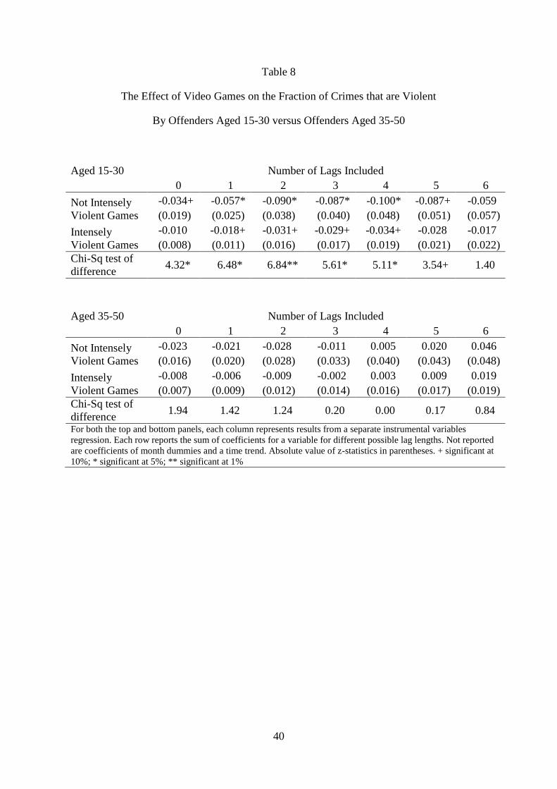
Table 8 reports cumulative estimates from estimating equation (2), where the
dependent variable is the logarithm of the fraction of crimes that are violent, for both these
younger and older groups. The specifications are otherwise identical to those reported in
Table 5 and again we report the estimated sum of effects over all lags as in Table 6. Now,
there are noticeable differences across the two groups. None of the estimates for the older
group approach traditional levels of statistical significance. In contrast, the estimates for the
younger group are generally larger (in absolute value) than those in the lower panel of Table 6
and more often reach statistical significance. In addition, the differences in estimates between
violent and nonviolent games are larger and are more often statistically significant. We again
find that, for the younger group, non-violent games, as well as violent games, reduce the
fraction of crimes that are violent. As before we are unsure what the mechanism is that would
lead non-violent games to reduce violent crimes, but we hypothesize that, in addition to this
mechanism, violent games also could increase gamers violent behaviors as indicated by the
laboratory experiments. In these specifications, this is measured by the difference between the
coefficients in the two rows which is measured to be as large as 0.07. Thus, this is evidence
that the behavioral effect of violent video games on violent behavior is found only within the
population that plays video games more intensively.
C. On Campus Results
Another potential robustness check is to distinguish between crimes committed at
schools and colleges and those committed elsewhere. Schools and colleges tend to aggregate
people who are of video game playing age. The NIBRS data record the location of each
incident as a categorical variable where one possible choice out of eleven is “school or college

24
campus.” One advantage of this variable over the age of offender variable is that it is recorded
for all incidents while the age of offender can be missing if no one witnessed the incident in
progress. One disadvantage is that crimes committed at schools and colleges need not be
committed by a member of the younger video game playing demographic, though most are.
Perhaps a bigger problem is that many of the younger video game playing population commit
crimes away from schools. Finally, since such a small number of crimes are committed on
campus, we may lose statistical power for that sub-sample while the off-campus sub-sample
will be quite similar to the overall sample.
Table 9 reports cumulative estimates from estimating equation (1) for both crimes
committed on campuses and those committed off-campus. The specifications are otherwise
identical to those reported in Table 4 but we report the estimated cumulative effect over all
lags as in Table 6. As before, specifications with lags from between two and five achieve
some level of statistical significance for both the young and the old. The pattern of estimated
effects for both violent and non-violent video games is similar to before except that they are
much larger for on-campus crimes than off-campus. In the lower panel, the estimates are
qualitatively similar to the base results in Table 6. However, the upper panel estimates are
about five times larger. Other than the difference in magnitudes, the pattern of effects on-
campus is unchanged. There is still a negative effect for non-violent video games in columns
2-5 that we interpret as an incapacitation effect. The estimated effect for violent video games
is statistically significantly smaller (in absolute value) and we interpret the difference as a
possible estimate of a behavioral effect of violent video games on crime.
Table 10 reports cumulative estimates from estimating equation (2), where the
dependent variable is the logarithm of the fraction of crimes that are violent, for both crimes
on and off campus. The specifications are otherwise identical to those reported in Table 2 and
again we report the estimated sum of effects over all lags as in Table 6. In this case, few

25
effects are estimated to be significantly different from zero. In contrast to before, non-violent
games may increase the violent composition of crimes on campus, holding all crimes constant
but only in column 1. As expected, the off-campus results are more similar our basic results
reported in the bottom panel of Table 6.
V. Conclusion
Regulation of the video game industry is usually predicated on the notion that the
industry has large and negative social costs through games‟ effect on aggression. Many
researchers have argued that these games may also have caused extreme violence, such as
school shootings, because laboratory evidence has found an abundance of evidence linking
gameplay to aggression. Yet few studies before this one had examined the impact of these
games on crime, with the exception of Ward (2011) and Dahl and Dellavegna (2009).
Consistent with these studies, we find that the social costs of violent video games may be
considerably lower, or even non-existent, once one incorporates the time use effect into
analysis.
These analyses are suggestive of the hypothesis that violent video games, like all video
games, paradoxically may reduce violence while increasing the aggressiveness of individuals
by simply shifting these individuals out of alternative activities where crime is more likely to
occur. Insofar as our findings suggest that the operating mechanism by which violent
gameplay causes crime to fall is the gameplay itself, and not the violence, then regulations
should be carefully designed so as to avoid inadvertently reducing the time intensity, or the
appeal, of video games.
Our findings also suggest unique challenges to game regulations. Because GAM
proposes that the individual playing violent video games is developing, accidentally, a biased

26
hermeneutic towards people wherein they believe they are in danger, then the decrease in
violent outcomes that we observe in our study – the incapacitation effect from time use – may
be masking the long-run harm to society if these violent behaviors are developing within
gamers. This suggests that regulation aimed at reducing violent imagery and content in games
could in the long-run reduce the aggression capital stock among gamers, but potentially also
cause crime to increase in the short-run if the marginal player is being drawn out of violent
activities. This may be too costly a tradeoff, and may not pass any cost-benefit test. But
another possibility is that individuals who play games could be regularly taught to recognize
these errors in their framing of situations, which theoretically would reduce the aggressive
capital and thus reduce any negative outcome that is determined by the amount of aggression
the person has built up, without losing the short-run gains from crime reduction.

27
References
Anderson, Craig A. (2004). “An update on the effects of playing violent video games,”
Journal of Adolescence 27, 113–122.
Anderson, Craig A, Douglas A. Gentile, Katherine E. Buckley. (2007) Violent video game
effects on children and adolescents: theory, research and public policy. Oxford
University Press, 1st edition.
Anderson, C. A. and B. J. Bushman. 2002. “Human aggression.” Annual Review of
Psychology, 53:27–51.
Angrist, J. D. (2006). “Instrumental variables methods in experimental criminological
research: what, why and how.” Journal of Experimental Criminology 2: 23–44.
Becker, Gary S. (1965). “A theory of the allocation of time.” Economic Journal 75 (299), pp.
493-517.
Becker, Gary and Kevin M. Murphy (1988). “A theory of rational addiction.” The Journal of
Political Economy 96: p. 675-700.
Berk, R (2005). “Randomized experiments as the bronze standard.” Journal of Experimental
Criminology. 1:417-433.
B. J. Bushman and C. A. Anderson (2002). “Violent video games and hostile expectations: a
test of the general aggression model.” Personality and Social Psychology Bulletin 28
(12): 1679-1686.
D. T. Campbell and J. C. Stanley (1963). Experimental and quasi-experimental designs for
research. Chicago: Rand McNally.
Card, David and Gordon B. Dahl (2011). “Family violence and football: the effect of
unexpected emotional cues on violent behaviour.” Quarterly Journal of Economics
(forthcoming).
Comstock, Anthony and J. M. Buckley (1883) Traps for the young. Republished in 1967 by
Beknap Press, First Edition edition.
Dahl, Gordon and Stefano DellaVigna (2009). “Does movie violence increase violent crime?”
Quarterly Journal of Economics, 124(2) 637–675.
Deaton, A. (2010). “Instruments, randomization, and learning about development.” Journal of
Economic Literature 48: 424–455.
Ferguson, C. J. and J. Kilburn (2008). “The public health risks of media violence: a meta-
analytic review.” The Journal of Pediatrics 154(4): 759−763.
Fisher, R. A. (1935). The design of experiments. Oliver and Boyd, Edinburgh.
Gould, E. D., B. A. Weinberg and D. B. Mustard (2002). “Crime rates and local labor market
opportunities in the united states: 1979–1997.” The Review of Economics and
Statistics 84(1): 45–61
Hadju David (2009), The ten-cent plague: the great comic-book scare and how it changed
america. New York: Farrar, Strauss and Giroux.

28
Harrison, G. W. and J. A. List (2004). “Field experiments.” Journal of Economic Literature
42(4): 1013-1059.
Heckman, J. and S. Urzua (2010) “Comparing IV with structural models: what simple IV can
and cannot identify.” Journal of Econometrics 156 (1): 27-37.
Imbens, G. W. (2010). Better LATE Than Nothing: Some Comments on Deaton (2009) and
Heckman and Urzua (2009). Journal of Economic Literature 48(2): 399-423.
Hilger, James, Greg Rafert and Sofia Villas-Boas (2010). “Expert opinion and the demand for
experience goods: an experimental approach in the retail wine market.” Review of Economics
& Statistics, forthcoming.
Jacob, B. A., and E. Moretti (2003). “Are idle hands the devil's workshop? incapacitation,
concentration, and juvenile crime.” The American Economic Review 93 (5): 1560-
1577.
Jacob, B. A., L. Lefgren and E Moretti (2007). “The dynamics of criminal behavior: evidence
from weather shocks.” Journal of Human Resources 42 (3): 489–527.
Kutner, Lawrence and Cheryl Olson (2008). Grand theft childhood: the surprising truth about
violent video games and what parents can do. Simon & Schuster.
Rantala, Ramona R and Thomas J. Edwards (2000). “Effects of NIBRS on crime statistics”.
NCJ Publication 178890. US Department of Justice.
Raphael, S. and R. Winter-Ebmer (2001). “Identifying the effect of unemployment on crime.”
Journal of Law and Economics 44: 259-283.
Reinstein, D. and C. Snyder (2005). “The influence of expert reviews on consumer demand
for experience goods: A case study of movie critics.” Journal of Industrial Economics
53(1): 27–51.
Rosenbaum, P. R. (2002) Observational studies. New York: Springer.
Rosenbaum, P. R. (2002). “Covariance adjustment in randomized experiments and
observational studies.” Statistical Science 17(3): 286–304.
Stinebrickner, Ralph Todd R. Stinebrickner (2008). “The causal effect of studying on
academic performance.” The B.E. Journal of Economic Analysis & Policy: Frontiers
8(1) Article 14.
Ward, Michael R. (2010). “Video games and adolescent fighting.” Journal of Law and
Economics, 53(3) 611-628.
Ward, Michael R. (2011). “Video games and crime.” Contemporary Economic Policy. 29(2)
261-273.
Zhu, Feng and Xiaoquan (Michael) Zhang (2010). “Impact of online consumer reviews on
sales: the moderating role of product and consumer characteristics.” Journal of
Marketing, Vol. 74 (March 2010), 133–148.

29
Figure 1

30
Figure 2

31
Figure 3

32
Figure 4

33
Table 1
Unit Sales of Video Games (millions) from VGChartz and ESA
Year VGChartz ESA Pct
2005 56.7 240.7 23.6%
2006 76.2 267.8 28.5%
2007 107.0 298.2 35.9%
2008 141.3 273.5 51.7%
VGChartz from authors‟ calculations and ESA from
http://www.theesa.com/facts/pdfs/VideoGames21stCentury_2010.pdf.

34
Table 2
The Effect of Game Quality (Game Spot Score) on Log Sales
All Intensely Violent Not Intensely Violent
Games Games Games
GameSpot
Score
0.0803** 0.1221** 0.0769**
(0.0060) (0.0181) (0.0065)
Week of
Release
-0.0039** -0.0081** -0.0036**
(0.0002) (0.0008) (0.0003)
Trend 0.0058** 0.0040** 0.0060**
(0.0001) (0.0003) (0.0001)
February -0.0902* -0.2169* -0.0663+
(0.0361) (0.1020) (0.0385)
March -0.0212 -0.0576 -0.0081
(0.0348) (0.0967) (0.0371)
April -0.1770** -0.3466** -0.1361**
(0.0344) (0.0945) (0.0369)
May -0.2838** -0.4069** -0.2485**
(0.0355) (0.1004) (0.0378)
June -0.1663** -0.3593** -0.1217**
(0.0363) (0.1036) (0.0386)
July -0.2251** -0.5266** -0.1732**
(0.0358) (0.1059) (0.0378)
August -0.3607** -0.6881** -0.3126**
(0.0364) (0.1151) (0.0381)
September -0.2700** -0.4117** -0.2422**
(0.0358) (0.1200) (0.0374)
October -0.1326** 0.0065 -0.1333**
(0.0365) (0.1159) (0.0383)
November 0.6122** 0.6812** 0.6051**
(0.0361) (0.1052) (0.0382)
December 1.2038** 1.1363** 1.2153**
(0.0349) (0.1073) (0.0367)
Constant -4.8503** -0.5994 -5.3472**
(0.2957) (0.8309) (0.3189)
Observations 10,648 1,345 9,303
R-squared 0.38 0.40 0.38
Standard errors in parentheses
+ significant at 10%; * significant at 5%; ** significant at 1%

35
Table 3
Summary Statistics
Variable Mean Std. Dev.
Ln All Video Game Sales 0.407 0.632
Ln Intensely Violent Video Game Sales -1.900 1.037
Ln Not Intensely Violent Video Game Sales 0.781 0.340
Average GameSpot Score 7.634 0.435
Average Intensely Violent GameSpot Score 8.546 0.646
Average Not Intensely Violent GameSpot Score 7.506 0.468
Ln All Crimes 10.889 0.085
Ln Violent Share of All Crimes 3.689 0.028
Ln All Crimes on Campuses 7.463 0.421
Ln Violent Share of All Crimes on Campuses 3.796 0.107
Ln All Crimes Not on Campuses 10.852 0.091
Ln Violent Share of All Crimes Not on Campuses 3.683 0.028
Ln All Crimes Offender Aged 15-30 9.854 0.068
Ln Violent Share of All Crimes Offender 15-30 4.117 0.024
Ln All Crimes Offender Aged 35-50 9.040 0.082
Ln Violent Share of All Crimes Offender 35-50 4.172 0.022
Descriptive statistics of the 200 observations used in later tables.

36
Table 4
The Effects of Video Game Sales on the Log of both Violent and Non-Violent Crime
(1) (2) (3) (4) (5) (6) (7)
Ln Video Game Sales
Not Intensely Violent
-0.028 0.029 0.030 0.041 0.042 0.032 0.044
(0.60) (0.50) (0.44) (0.54) (0.52) (0.40) (0.55)
Ln VG Sales Not
Intensely Violent lag 1
-0.130+ -0.110 -0.090 -0.089 -0.099 -0.088
(1.92) (1.35) (1.03) (1.03) (1.15) (1.02)
Ln VG Sales Not
Intensely Violent lag 2
-0.131+ -0.098 -0.095 -0.044 -0.040
(1.71) (1.16) (1.13) (0.50) (0.46)
Ln VG Sales Not
Intensely Violent lag 3
-0.068 -0.067 -0.064 -0.075
(0.91) (0.88) (0.86) (0.90)
Ln VG Sales Not
Intensely Violent lag 4
0.010 0.042 0.029
(0.12) (0.53) (0.35)
Ln VG Sales Not
Intensely Violent lag 5
-0.125+ -0.126+
(1.73) (1.72)
Ln VG Sales Not
Intensely Violent lag 6
0.026
(0.30)
Ln Intensely Violent
Video Game Sales
-0.009 0.014 0.019 0.030 0.031 0.023 0.026
(0.44) (0.56) (0.64) (0.94) (0.94) (0.71) (0.81)
Ln Intensely Violent
VG Sales lag 1
-0.055+ -0.043 -0.029 -0.029 -0.034 -0.027
(1.77) (1.11) (0.70) (0.69) (0.83) (0.65)
Ln Intensely Violent
VG Sales lag 2
-0.063+ -0.044 -0.042 -0.021 -0.017
(1.72) (1.06) (1.02) (0.49) (0.39)
Ln Intensely Violent
VG Sales lag 3
-0.048 -0.047 -0.047 -0.051
(1.41) (1.27) (1.29) (1.22)
Ln Intensely Violent
VG Sales lag 4
0.001 0.011 0.006
(0.04) (0.29) (0.15)
Ln Intensely Violent
VG Sales lag 5
-0.036 -0.032
(1.10) (0.91)
Ln Intensely Violent
VG Sales lag 6
-0.000
(0.01)
Sample includes 200 weekly observations from 2004-2008. Month dummy variables and a time trend were also
included but are not reported. Average GameSpot scores for intensely violent and not for the current period and eight
lags are used as IVs. The Sargon statistic for over-identification always fails to reject the exogeneity of the instrument
set. Absolute value of z-statistics in parentheses. + significant at 10%; * significant at 5%; ** significant at 1%.

37
Table 5
The Effects of Video Game Sales on the Log of the Fraction of Crime that is Violent
(1) (2) (3) (4) (5) (6) (7)
Ln Video Game Sales
Not Intensely Violent
-0.033+ -0.024 -0.020 -0.043 -0.041 -0.047 -0.050
(1.72) (1.05) (0.78) (1.51) (1.39) (1.48) (1.55)
Ln VG Sales Not
Intensely Violent lag 1
-0.021 -0.023 -0.014 -0.013 -0.013 -0.017
(0.77) (0.79) (0.43) (0.40) (0.37) (0.50)
Ln VG Sales Not
Intensely Violent lag 2
-0.015 -0.038 -0.036 -0.053 -0.051
(0.53) (1.21) (1.15) (1.52) (1.41)
Ln VG Sales Not
Intensely Violent lag 3
0.065* 0.067* 0.070* 0.064+
(2.34) (2.36) (2.33) (1.87)
Ln VG Sales Not
Intensely Violent lag 4
0.001 -0.010 0.000
(0.04) (0.31) (0.00)
Ln VG Sales Not
Intensely Violent lag 5
0.052+ 0.048
(1.79) (1.59)
Ln VG Sales Not
Intensely Violent lag 6
0.014
(0.40)
Ln Intensely Violent
Video Game Sales
-0.015+ -0.015 -0.015 -0.022+ -0.021+ -0.023+ -0.023+
(1.88) (1.45) (1.38) (1.84) (1.70) (1.72) (1.71)
Ln Intensely Violent
VG Sales lag 1
-0.004 -0.006 -0.000 0.000 -0.001 -0.004
(0.36) (0.43) (0.01) (0.01) (0.07) (0.24)
Ln Intensely Violent
VG Sales lag 2
-0.003 -0.017 -0.016 -0.023 -0.023
(0.26) (1.13) (1.06) (1.36) (1.30)
Ln Intensely Violent
VG Sales lag 3
0.026* 0.028* 0.029* 0.025
(2.03) (2.01) (1.99) (1.47)
Ln Intensely Violent
VG Sales lag 4
-0.002 -0.010 -0.006
(0.14) (0.69) (0.35)
Ln Intensely Violent
VG Sales lag 5
0.025+ 0.021
(1.93) (1.44)
Ln Intensely Violent
VG Sales lag 6
0.011
(0.63)
Sample includes 200 weekly observations from 2004-2008. Month dummy variables and a time trend were also
included but are not reported. Average GameSpot scores for intensely violent and not for eight lags are used as IVs.
The Sargon statistic for over-identification always fails to reject the exogeneity of the instrument set. Absolute
value of z-statistics in parentheses. + significant at 10%; * significant at 5%; ** significant at 1%.

38
Table 6
The Cumulative Effect of Video Games on Crimes
Aggregate Effect on all Crimes (from Table 1)
Number of Lags Included
0 1 2 3 4 5 6
Not Intensely
Violent Coefs.
-0.028 -0.101 -0.210* -0.214* -0.200 -0.256* -0.229
(0.046) (0.062) (0.096) (0.105) (0.122) (0.124) (0.140)
Intensely
Violent Coefs.
-0.009 -0.041 -0.087* -0.092* -0.086+ -0.104* -0.095
(0.020) (0.027) (0.040) (0.044) (0.049) (0.050) (0.056)
Chi-Sq test of
difference 0.44 2.67 4.69* 3.76+ 2.33 4.07* 2.46
Aggregate Effect on all Fraction of Crimes that are Violent (from Table 2)
Violent/
All Crimes
Number of Lags Included
0 1 2 3 4 5 6
Not Intensely
Violent Games
-0.033+ -0.045+ -0.058+ -0.030 -0.022 -0.001 0.007
(0.019) (0.025) (0.035) (0.039) (0.045) (0.050) (0.057)
Intensely
Violent Games
-0.015+ -0.019+ -0.024+ -0.014 -0.011 0.002 0.001
(0.008) (0.011) (0.015) (0.016) (0.018) (0.020) (0.022)
Chi-Sq test of
difference 2.22 2.95+ 2.60 0.48 0.17 0.00 0.03
For both the top and bottom panels, each column represents results from a separate instrumental variables
regression. Each row reports the sum of coefficients for a variable for different possible lag lengths. Not
reported are coefficients of month dummies and a time trend. Absolute value of z-statistics in parentheses. +
significant at 10%; * significant at 5%; ** significant at 1%

39
Table 7
The Effect of Video Games on both Violent and Non-Violent Crimes
By Offenders Aged 15-30 versus Offenders Aged 35-50
Aged 15-30 Number of Lags Included
0 1 2 3 4 5 6
Not Intensely
Violent Games
-0.028 -0.098 -0.182* -0.178+ -0.167 -0.218+ -0.214
(0.046) (0.061) (0.092) (0.100) (0.115) (0.117) (0.134)
Intensely
Violent Games
-0.012 -0.043 -0.079* -0.081+ -0.077+ -0.093* -0.093+
(0.019) (0.026) (0.039) (0.042) (0.046) (0.047) (0.054)
Chi-Sq test of
difference 0.32 2.31 3.56+ 2.62 1.66 3.04+ 2.18
Aged 35-50 Number of Lags Included
0 1 2 3 4 5 6
Not Intensely
Violent Games
-0.020 -0.089 -0.236* -0.210+ -0.214 -0.243+ -0.235
(0.049) (0.068) (0.112) (0.117) (0.136) (0.138) (0.157)
Intensely
Violent Games
-0.014 -0.042 -0.103* -0.096* -0.098+ -0.105+ -0.102
(0.021) (0.029) (0.047) (0.049) (0.055) (0.056) (0.062)
Chi-Sq test of
difference 0.05 1.37 4.01* 2.63 1.99 2.69 1.91
For both the top and bottom panels, each column represents results from a separate instrumental variables
regression. Each row reports the sum of coefficients for a variable for different possible lag lengths. Not reported
are coefficients of month dummies and a time trend. Absolute value of z-statistics in parentheses. + significant at
10%; * significant at 5%; ** significant at 1%
40
Table 8
The Effect of Video Games on the Fraction of Crimes that are Violent
By Offenders Aged 15-30 versus Offenders Aged 35-50
Aged 15-30 Number of Lags Included
0 1 2 3 4 5 6
Not Intensely
Violent Games
-0.034+ -0.057* -0.090* -0.087* -0.100* -0.087+ -0.059
(0.019) (0.025) (0.038) (0.040) (0.048) (0.051) (0.057)
Intensely
Violent Games
-0.010 -0.018+ -0.031+ -0.029+ -0.034+ -0.028 -0.017
(0.008) (0.011) (0.016) (0.017) (0.019) (0.021) (0.022)
Chi-Sq test of
difference 4.32* 6.48* 6.84** 5.61* 5.11* 3.54+ 1.40
Aged 35-50 Number of Lags Included
0 1 2 3 4 5 6
Not Intensely
Violent Games
-0.023 -0.021 -0.028 -0.011 0.005 0.020 0.046
(0.016) (0.020) (0.028) (0.033) (0.040) (0.043) (0.048)
Intensely
Violent Games
-0.008 -0.006 -0.009 -0.002 0.003 0.009 0.019
(0.007) (0.009) (0.012) (0.014) (0.016) (0.017) (0.019)
Chi-Sq test of
difference 1.94 1.42 1.24 0.20 0.00 0.17 0.84
For both the top and bottom panels, each column represents results from a separate instrumental variables
regression. Each row reports the sum of coefficients for a variable for different possible lag lengths. Not reported
are coefficients of month dummies and a time trend. Absolute value of z-statistics in parentheses. + significant at
10%; * significant at 5%; ** significant at 1%

41
Table 9
The Aggregate Effect of Video Games on both Violent and Non-Violent Crimes
By Crimes Located at Schools and Not at Schools
Crimes on
Campus
Number of Lags Included
0 1 2 3 4 5 6
Not Intensely
Violent Games
-0.050 -0.442 -0.841* -1.135* -1.108+ -1.396* -0.976
(0.265) (0.307) (0.415) (0.484) (0.567) (0.595) (0.724)
Intensely
Violent Games
0.016 -0.177 -0.342* -0.468* -0.461* -0.563* -0.399
(0.112) (0.132) (0.175) (0.202) (0.230) (0.240) (0.289)
Chi-Sq test of
difference 0.16 2.06 4.07* 5.24* 3.50+ 5.24* 1.70
Crimes off
Campus
Number of Lags Included
0 1 2 3 4 5 6
Not Intensely
Violent Games
-0.024 -0.086 -0.189* -0.185+ -0.171 -0.221+ -0.207
(0.045) (0.061) (0.094) (0.103) (0.120) (0.121) (0.137)
Intensely
Violent Games
-0.008 -0.035 -0.078* -0.080+ -0.075 -0.090+ -0.087
(0.019) (0.026) (0.040) (0.043) (0.048) (0.049) (0.055)
Chi-Sq test of
difference 0.31 2.00 3.87* 2.87+ 1.73 3.13+ 2.06
For both the top and bottom panels, each column represents results from a separate instrumental variables
regression. Each row reports the sum of coefficients for a variable for different possible lag lengths. Not
reported are coefficients of month dummies and a time trend. Absolute value of z-statistics in parentheses. +
significant at 10%; * significant at 5%; ** significant at 1%

42
Table 10
The Effect of Video Games on the Fraction of Crimes that are Violent
By Crimes Located at Schools and Not at Schools
Crimes on
Campus Number of Lags Included
0 1 2 3 4 5 6
Not Intensely
Violent Games
0.086 0.057 0.077 0.072 0.141 0.111 0.165
(0.057) (0.070) (0.098) (0.104) (0.123) (0.132) (0.158)
Intensely
Violent Games
0.020 0.002 0.012 0.009 0.034 0.026 0.049
(0.024) (0.030) (0.042) (0.043) (0.050) (0.053) (0.063)
Chi-Sq test of
difference 3.54+ 1.65 1.23 1.02 2.03 1.12 1.43
Crimes off
Campus Number of Lags Included
0 1 2 3 4 5 6
Not Intensely
Violent Games
-0.037+ -0.047+ -0.061+ -0.030 -0.024 -0.000 0.007
(0.020) (0.026) (0.037) (0.042) (0.048) (0.054) (0.061)
Intensely
Violent Games
-0.016+ -0.020+ -0.025 -0.013 -0.011 -0.002 0.001
(0.009) (0.011) (0.015) (0.017) (0.020) (0.022) (0.025)
Chi-Sq test of
difference 2.58 3.06+ 2.68 0.46 0.19 0.00 0.02
For both the top and bottom panels, each column represents results from a separate instrumental variables
regression. Each row reports the sum of coefficients for a variable for different possible lag lengths. Not
reported are coefficients of month dummies and a time trend. Absolute value of z-statistics in parentheses. +
significant at 10%; * significant at 5%; ** significant at 1%


![Teens & Video Games - BubbleUp Classroom€¦ · “Playing [violent video games] can and does stir hostile urges and mildly aggressive behavior in the short term. Moreover, youngsters](https://img.pdfslide.us/doc/110x75/5f057e147e708231d4133b72/teens-video-games-bubbleup-classroom-aoeplaying-violent-video-games-can.jpg)