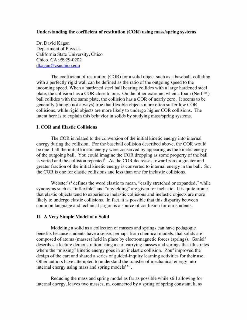
Understanding the coefficient of restitution (COR) using mass/spring systems Dr. David Kagan Department of Physics California State University, Chico Chico, CA 95929-0202 dkagan@csuchico.edu

The coefficient of restitution (COR) for a solid object such as a baseball, colliding with a perfectly rigid wall can be defined as the ratio of the outgoing speed to the incoming speed. When a hardened steel ball bearing collides with a large hardened steel plate, the collision has a COR close to one. On the other extreme, when a foam (Nerft™) ball collides with the same plate, the collision has a COR of nearly zero. It seems to be generally (though not always) true that flexible objects more often suffer low COR collisions, while rigid objects are more likely to undergo higher COR collisions. The intent here is to explain this behavior in solids by studying mass/spring systems.

I. COR and Elastic Collisions

The COR is related to the conversion of the initial kinetic energy into internal

energy during the collision. For the baseball collision described above, the COR would be one if all the initial kinetic energy were conserved by appearing as the kinetic energy of the outgoing ball. You could imagine the COR dropping as some property of the ball is varied and the collision repeated1. As the COR decreases toward zero, a greater and greater fraction of the initial kinetic energy is converted to internal energy in the ball. So, the COR is one for elastic collisions and less than one for inelastic collisions.

Webster’s2 defines the word elastic to mean, “easily stretched or expanded,” while

synonyms such as “inflexible” and “unyielding” are given for inelastic. It is quite ironic that elastic objects tend to experience inelastic collisions and inelastic objects are more likely to undergo elastic collisions. In fact, it is possible that this disparity between common language and technical jargon is a source of confusion for our students.

II. A Very Simple Model of a Solid Modeling a solid as a collection of masses and springs can have pedagogic benefits because students have a sense, perhaps from chemical models, that solids are composed of atoms (masses) held in place by electromagnetic forces (springs). Ganiel3 describes a lecture demonstration using a cart carrying masses and springs that illustrates where the “missing” kinetic energy goes in an inelastic collision. Zou4 improved the design of the cart and shared a series of guided-inquiry learning activities for their use. Other authors have attempted to understand the transfer of mechanical energy into internal energy using mass and spring models5,6,7.

Reducing the mass and spring model as far as possible while still allowing for internal energy, leaves two masses, m, connected by a spring of spring constant, k, as

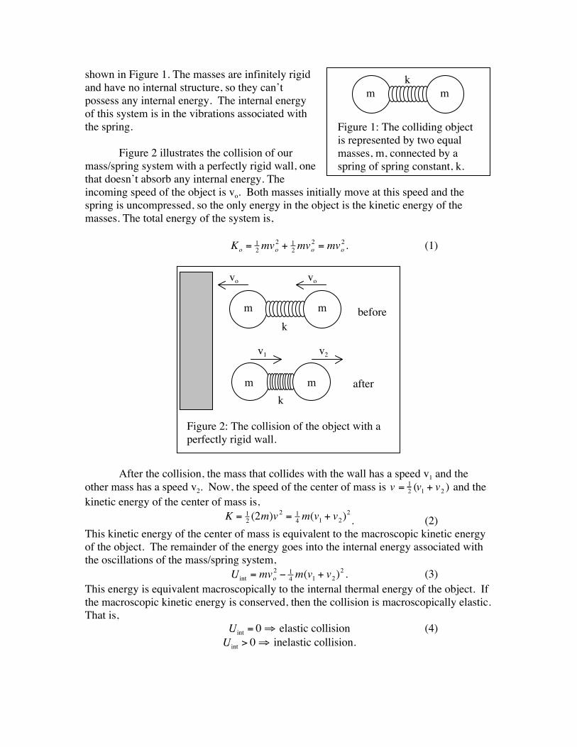
shown in Figure 1. The masses are infinitely rigid and have no internal structure, so they can’t possess any internal energy. The internal energy of this system is in the vibrations associated with the spring. Figure 2 illustrates the collision of our mass/spring system with a perfectly rigid wall, one that doesn’t absorb any internal energy. The incoming speed of the object is vo. Both masses initially move at this speed and the spring is uncompressed, so the only energy in the object is the kinetic energy of the masses. The total energy of the system is,

€

Ko = 12mvo

2 + 12mvo

2 = mvo2. (1)

After the collision, the mass that collides with the wall has a speed v1 and the

other mass has a speed v2. Now, the speed of the center of mass is

€

v = 12 (v1 + v2 ) and the

kinetic energy of the center of mass is,

€

K = 12 (2m)v

2 = 14 m(v1 + v2)

2. (2)

This kinetic energy of the center of mass is equivalent to the macroscopic kinetic energy of the object. The remainder of the energy goes into the internal energy associated with the oscillations of the mass/spring system,

€

U int = mvo2 − 1

4 m(v1 + v2)2 . (3)

This energy is equivalent macroscopically to the internal thermal energy of the object. If the macroscopic kinetic energy is conserved, then the collision is macroscopically elastic. That is,

€

Uint = 0⇒ elastic collision (4)

€

Uint > 0⇒ inelastic collision.

k

Figure 1: The colliding object is represented by two equal masses, m, connected by a spring of spring constant, k.

m m

k

vo vo

k

v1 v2

before

after

Figure 2: The collision of the object with a perfectly rigid wall.

m m

m m

The COR of the collision is the ratio of the center of mass velocity after the collision to the center of mass velocity before,

€

COR = −vcm, fvcm,i

= −12 (v1 + v2)12 (vo + vo)

= −v1 + v22vo

. (5)

The COR can be related directly to the kinetic energies,

€

COR =KKo

. (6)

Therefore, the COR is one for elastic collisions. As the COR gets smaller, more and more of the initial kinetic energy is converted to the internal energy in the mass/spring system resulting in a COR less than one. For the remainder of this discussion we will focus on the COR keeping in mind that it is a surrogate for the energy transferred to internal energy. III. A Naïve Model of a Collision

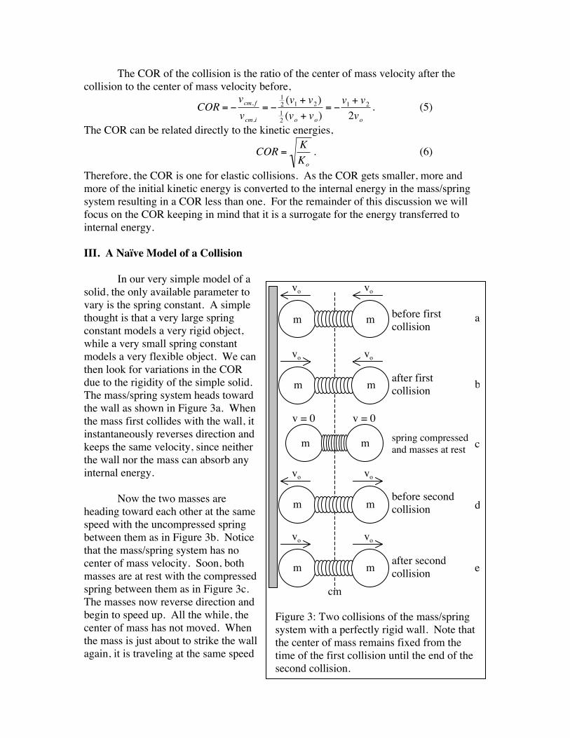
In our very simple model of a solid, the only available parameter to vary is the spring constant. A simple thought is that a very large spring constant models a very rigid object, while a very small spring constant models a very flexible object. We can then look for variations in the COR due to the rigidity of the simple solid. The mass/spring system heads toward the wall as shown in Figure 3a. When the mass first collides with the wall, it instantaneously reverses direction and keeps the same velocity, since neither the wall nor the mass can absorb any internal energy.

Now the two masses are heading toward each other at the same speed with the uncompressed spring between them as in Figure 3b. Notice that the mass/spring system has no center of mass velocity. Soon, both masses are at rest with the compressed spring between them as in Figure 3c. The masses now reverse direction and begin to speed up. All the while, the center of mass has not moved. When the mass is just about to strike the wall again, it is traveling at the same speed

Figure 3: Two collisions of the mass/spring system with a perfectly rigid wall. Note that the center of mass remains fixed from the time of the first collision until the end of the second collision.

cm

vo vo

before first collision

a m m

vo vo

before second collision d m m

vo vo

after first collision b m m

vo vo

after second collision e m m

v = 0 v = 0

spring compressed and masses at rest c m m

it had before the first collision. Meanwhile the other mass has the same speed as before, but has reversed direction as shown in Figure 3d. The spring is now uncompressed. The mass collides with the wall and reverses direction again. Now, both masses are headed away from the wall with the same speed as they arrived and the spring is uncompressed between them as in Figure 3e.

The COR for this collision appears to be zero after the first bounce off the wall

because the center of mass of the system in Figures 3b, 3c, and 3d is at rest and all of the energy is in the internal motion of the mass/spring system. However, after the second bounce, the COR is one and the collision is elastic regardless of the spring constant. Our naïve idea that the rigidity of an object can be modeled by varying the internal spring constant seems doomed8. However, the force exerted by the wall on the mass during the collision is actually far more complex than the instantaneous impulse we have assumed. The “devil is in the details” of the collision which can be modeled using the speed of compressional waves that travel along the spring. Roura9 presents a very clean conceptual discussion of this issue. IV. Toward a Better Model

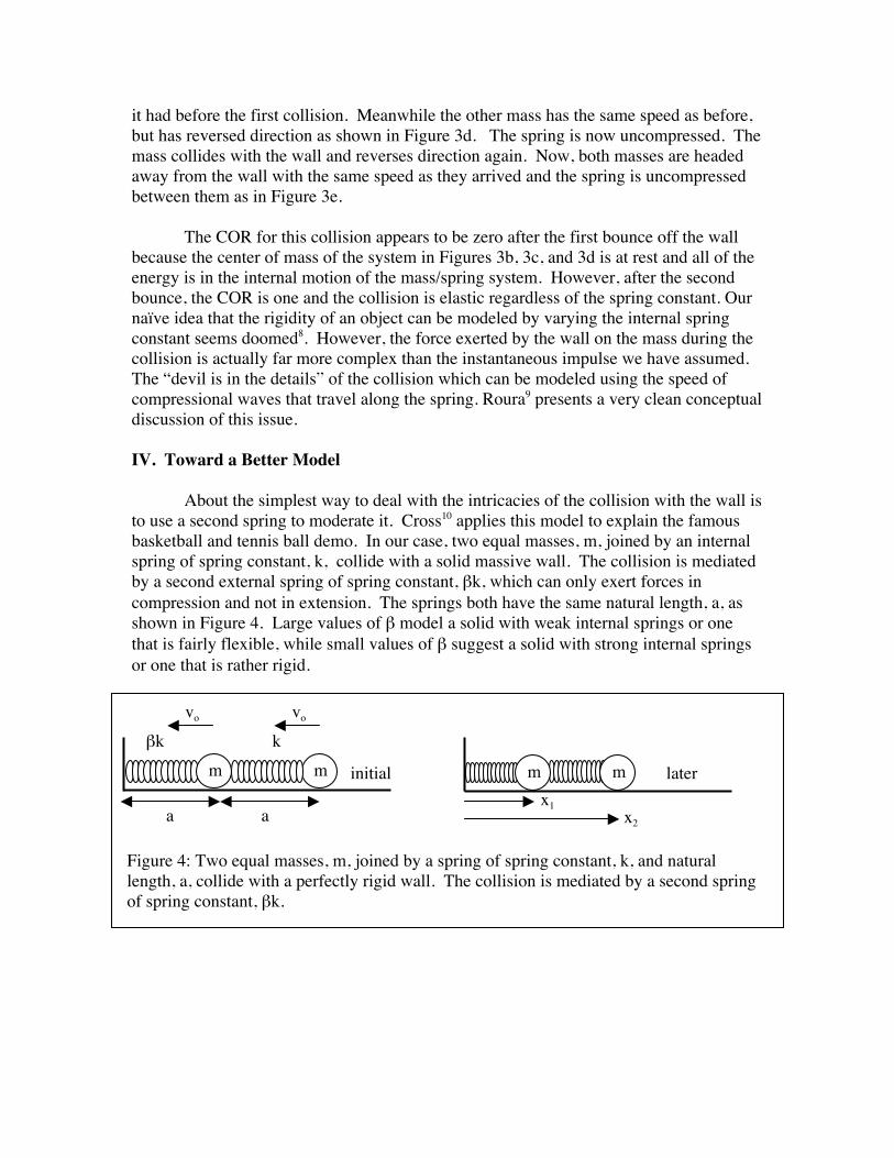
About the simplest way to deal with the intricacies of the collision with the wall is

to use a second spring to moderate it. Cross10 applies this model to explain the famous basketball and tennis ball demo. In our case, two equal masses, m, joined by an internal spring of spring constant, k, collide with a solid massive wall. The collision is mediated by a second external spring of spring constant, βk, which can only exert forces in compression and not in extension. The springs both have the same natural length, a, as shown in Figure 4. Large values of β model a solid with weak internal springs or one that is fairly flexible, while small values of β suggest a solid with strong internal springs or one that is rather rigid.

m m βk

k

a a

vo vo

initial m m x1

x2

later

Figure 4: Two equal masses, m, joined by a spring of spring constant, k, and natural length, a, collide with a perfectly rigid wall. The collision is mediated by a second spring of spring constant, βk.

The goal is to follow the motion of the system until it stops interacting with the wall (x1 > a). Then find the center of mass speed of the system to calculate the COR for the collision. Writing Newton’s Second Law for each mass when x1 < a,

€

m d2x1dt 2

= βk(a − x1) − k[a − (x2 − x1)] (7)

€

m d2x2dt 2

= +k[a − (x2 − x1)]. (8)

When the system is not interacting with the wall (x1 > a), the Second Law equations are the same except β = 0. Equations 7 and 8 are subject to the initial conditions,

€

x1(0) = a,

€

x2(0) = 2a ,

€

˙ x 1(0) = −vo , and

€

˙ x 2(0) = −vo. (9) If you are enamored with elegance, closed form

solutions, and advanced mathematics, you can solve these equations by the method of normal modes11. If you are less skilled and willing to tolerate numerical round off errors, you can solve them numerically. This author naturally chose the later.

By varying the value of β, you can go from a

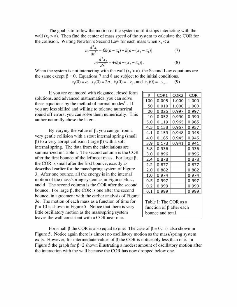
very gentle collision with a stout internal spring (small β) to a very abrupt collision (large β) with a soft internal spring. The data from the calculations are summarized in Table I. The second column is the COR after the first bounce of the leftmost mass. For large β, the COR is small after the first bounce, exactly as described earlier for the mass/spring system of Figure 3. After one bounce, all the energy is in the internal motion of the mass/spring system as in Figures 3b, c, and d. The second column is the COR after the second bounce. For large β, the COR is one after the second bounce, in agreement with the earlier analysis of Figure 3e. The motion of each mass as a function of time for β = 10 is shown in Figure 5. Notice that there is very little oscillatory motion as the mass/spring system leaves the wall consistent with a COR near one.

For small β the COR is also equal to one. The case of β = 0.1 is also shown in Figure 5. Notice again there is almost no oscillatory motion as the mass/spring system exits. However, for intermediate values of β the COR is noticeably less than one. In Figure 5 the graph for β=2 shown illustrating a modest amount of oscillatory motion after the interaction with the wall because the COR has now dropped below one.

β COR1 COR2 COR 100 0.005 1.000 1.000 50 0.010 1.000 1.000 20 0.025 0.997 0.997 10 0.052 0.990 0.990

5.0 0.119 0.965 0.965 4.5 0.138 0.957 0.957 4.1 0.159 0.948 0.948 4.0 0.165 0.945 0.945 3.9 0.173 0.941 0.941 3.8 0.936 0.936 3.0 0.896 0.896 2.4 0.878 0.878 2.2 0.877 0.877 2.0 0.882 0.882 1.0 0.974 0.974 0.5 0.997 0.997 0.2 0.999 0.999 0.1 0.999 0.999 Table I: The COR as a function of β after each bounce and total.

COR vs. β

0.8 0.82 0.84 0.86 0.88 0.9

0.92 0.94 0.96 0.98

1

0.1 1 10 100 β

COR

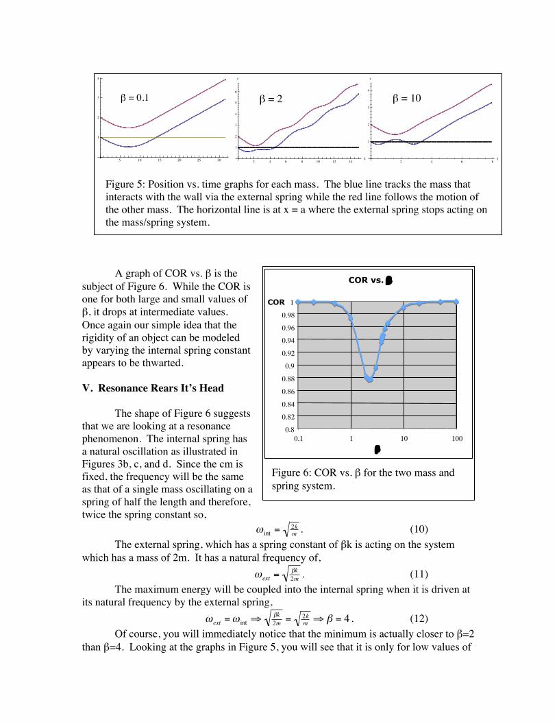
Figure 6: COR vs. β for the two mass and spring system.

A graph of COR vs. β is the

subject of Figure 6. While the COR is one for both large and small values of β, it drops at intermediate values. Once again our simple idea that the rigidity of an object can be modeled by varying the internal spring constant appears to be thwarted.

V. Resonance Rears It’s Head

The shape of Figure 6 suggests

that we are looking at a resonance phenomenon. The internal spring has a natural oscillation as illustrated in Figures 3b, c, and d. Since the cm is fixed, the frequency will be the same as that of a single mass oscillating on a spring of half the length and therefore, twice the spring constant so,

€

ω int = 2km . (10)

The external spring, which has a spring constant of βk is acting on the system which has a mass of 2m. It has a natural frequency of,

€

ωext = βk2m . (11)

The maximum energy will be coupled into the internal spring when it is driven at its natural frequency by the external spring,

€

ωext =ω int ⇒βk2m = 2k

m ⇒β = 4 . (12) Of course, you will immediately notice that the minimum is actually closer to β=2

than β=4. Looking at the graphs in Figure 5, you will see that it is only for low values of

5 10 15 20 25 30

1

2

3

4

2 4 6 8t

1

2

3

4

x

2 4 6 8 10 12 14t

1

2

3

4

5

6

x

β = 10 β = 0.1 β = 2

Figure 5: Position vs. time graphs for each mass. The blue line tracks the mass that interacts with the wall via the external spring while the red line follows the motion of the other mass. The horizontal line is at x = a where the external spring stops acting on the mass/spring system.

β that the motion of the external spring is close to simple harmonic. For higher values of β the motion is more complex and therefore so is the force exerted by the external spring on the mass/spring system. The mass/spring system could be treated as a forced harmonic oscillator.

VI. The Forced Harmonic Oscillator

To treat the mass/spring system as a forced oscillator let’s go back to the Second

Law equations (equations 7 and 8) and replace the external spring with a time dependent force,

€

m d2x1dt 2

= F(t) − k[a − (x2 − x1)] (13)

€

m d2x2dt 2

= +k[a − (x2 − x1)]. (14)

Rewriting in terms of the center of mass and the displacement of the masses from their equilibrium separation,

€

xcm ≡x1 +x22 and

€

xrel ≡ a − (x2 − x1) . (15) The Second Law equations become,

€

2m d2xcmdt 2

= F(t) and (16)

€

m d2xreldt 2

+ 2kxrel = F(t) . (17)

Equation 16 is simply a statement that the force exerted by the wall, F(t) , divided by the total mass, 2m, is equal to the acceleration of the center of mass. Newton would be pleased. Equation 17 is the equation for the forced oscillation of our oscillator, which has a natural frequency of

€

2km , in agreement with Equation 10. The energy absorbed by

the mass/spring system during the collision will appear as oscillations at this resonant frequency.

At this point we could begin the traditional forced oscillator problem12. However, that complex mathematics will obscure the point. We just need to understand that the force exerted on the mass/spring system transmitted by the external spring, F(t), changes the center of mass motion of the system and excites oscillations within the system. This forcing function contains different frequencies. The amount of oscillation excited depends upon the amount of the resonant frequency contained in the forcing function. As a result, we should not be surprised that Equation 12 only gives an approximate prediction for the frequency of the minimum COR.

The interaction with the wall causing resonant oscillations in the mass/spring system not only explains the location of the COR minimum, it explains the low β (strong internal spring) and high β (weak internal spring) results. For low β, the internal spring is strong and has a high resonant frequency. The weak external spring means a long collision time with the wall, so the forcing function is predominantly composed of a few low frequencies. The result is a mismatch with the high resonant frequency of the oscillator, very little oscillation will be excited, and a COR will be near one.

For high β it is a bit more complicated. The internal spring is weak and has a low resonant frequency. The strong external spring has a very short collision time with the wall, so the forcing function is composed of broad collection of frequencies some of which are bound to be close enough to the resonant frequency of the oscillator causing oscillations in the system. These can be seen in Table I after the first bounce, the COR is small.

However, the system interacts with the wall a second time. The time at which this happens is predominantly determined by the oscillation time of the internal spring. The second collision again results in a forcing function that has the same broad collection of frequencies some of which are again close enough to the resonant frequency of the internal spring. However, since the internal spring in now nearly half way through it’s oscillation, this second excitation is almost exactly out of phase with the first, canceling the oscillatory motion resulting in a COR that is close to one. This is essentially the message of figure 3.

Our two-mass/one-spring system has only one natural frequency,

€

2km . Since the

forcing function is a composed of a collection of frequencies, if we allow our system to have more natural resonances, something interesting is bound to happen. VII. More Masses and Springs We can create more natural resonances, if we add more masses and springs to our system. So, let the fun begin! Each time we add a spring and a mass to the right hand side we add another coupled equation to the equations of motion. This creates an additional natural frequency and increases the complexity of the forcing function. Since we don’t actually need the normal mode frequencies anyway (we just need to understand that they exist) and we have been able to use numerical solutions to this point, let’s just madly calculate. The result is the COR versus β curve shown in Figure 7. Each added natural frequency allows the mass/spring system to absorb more internal energy because of the added natural frequency. In the three mass system you can begin to see that the COR for high β is no longer tending toward one. By the time you get to four masses, the strongly suggestive single resonance shape of the two-mass system is entirely gone. At last, we begin to see the general trend we have been seeking, rigid low β objects tending to have higher COR’s than flexible high β objects. All the curves show some structural features owing to the natural resonances of the system.

For low β, the internal springs are strong and have a collection of high resonant frequencies. The weak external spring means a long collision time with the wall, so the forcing function is predominantly composed of low frequencies. The result is a mismatch with the high resonant frequencies of the oscillator, very little oscillation will be excited, and a COR will be near one regardless of the number of masses and springs.

For high β, the internal springs are weak and have a collection of low resonant

frequencies. The strong external spring has a short collision time with the wall, so the forcing function is composed of broad collection of frequencies some of which are close enough to the resonant frequencies of the oscillator to cause oscillations in the system.

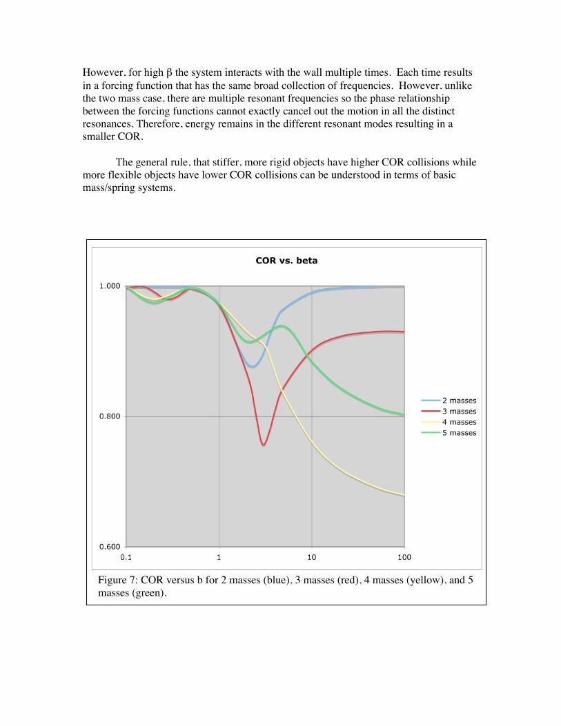
However, for high β the system interacts with the wall multiple times. Each time results in a forcing function that has the same broad collection of frequencies. However, unlike the two mass case, there are multiple resonant frequencies so the phase relationship between the forcing functions cannot exactly cancel out the motion in all the distinct resonances. Therefore, energy remains in the different resonant modes resulting in a smaller COR.

The general rule, that stiffer, more rigid objects have higher COR collisions while

more flexible objects have lower COR collisions can be understood in terms of basic mass/spring systems.

Figure 7: COR versus b for 2 masses (blue), 3 masses (red), 4 masses (yellow), and 5 masses (green).

1 D. T. Kagan, “The coefficient of restitution of baseballs as a function of relative humidity” Phys. Teach. 42, 330 (2004). 2 Webster’s New Collegiate Dictionary (G. & C. Merriam Co., Springfield, MA, 1974). 3 U. Ganiel, “Elastic and inelastic collisions: A model,” Phys. Teach. 30, 18-19 (1992). 4 X. Zou, “Making internal thermal energy visible” Phys. Teach. 42, 343-345(2003). 5 N. D. Newby Jr., “Linear collisions with harmonic oscillator forces: The inverse scattering problem,” Am. J. Phys., 47 (2), 161-165 (1979). 6 J. M. Aguirregabiria, A. Hernandez, and M. Rivas, “A simple model for inelastic collisions,” Am. J. Phys., 76 (11), 1071-1073 (2008). 7 R. Gruebel, J. Dennis, and L. Choate, “A variable coefficient of restitution experiment on a linear air track,” Am. J. Phys., 39 (4), 447-449 (1971). Actually this paper uses a pendulum to represent the internal energy. 8 Reference 4 uses the naïve model and gets interesting results. However, instead of varying the spring constant, the mass of the non-colliding ball is varied. This is unsatisfying because this model makes it appear as though the COR depends upon the mass of the colliding object. The same holds for reference 5 where the COR depends upon the mass at the end of the pendulum that represents the internal energy. 9 P. Roura, “Collision Duration in the Elastic Regime,” Phys. Teach. 35, 435-436 (1997). 10 R. Cross, “Vertical bounce of two vertically aligned balls,” Am. J. Phys., 75 (11), 1009-1016 (2007). 11 F. S. Crawford, Waves – Berkeley Physics Course v.3 (McGraw-Hill, New York, 1968), pp. 101-154. 12M. L. Boas, Mathematical Methods in the Physical Sciences (John Wiley & Sons, New York, 1966), pp. 348-350