Understanding terrestrial water storage variations in ...pubman.mpdl.mpg.de/pubman/item/escidoc:2506137:6/component/es… · 4064 T. Trautmann et al.: Understanding terrestrial water

Hydrol. Earth Syst. Sci., 22, 4061–4082, 2018https://doi.org/10.5194/hess-22-4061-2018© Author(s) 2018. This work is distributed underthe Creative Commons Attribution 4.0 License.

Understanding terrestrial water storage variationsin northern latitudes across scalesTina Trautmann1,2, Sujan Koirala1, Nuno Carvalhais1,3, Annette Eicker4, Manfred Fink5, Christoph Niemann1,5, andMartin Jung1

1Department of Biogeochemical Integration, Max-Planck-Institute for Biogeochemistry, 07745 Jena, Germany2International Max Planck Research School for Global Biogeochemical Cycles, 07745 Jena, Germany3CENSE, Departamento de Ciências e Engenharia do Ambiente, Faculdade de Ciências e Tecnologia,Universidade Nova de Lisboa, Caparica, 2829-516, Portugal4HafenCity University, 20457 Hamburg, Germany5Department of Geography, Friedrich-Schiller University, 07743 Jena, Germany

Correspondence: Tina Trautmann ([email protected])

Received: 27 November 2017 – Discussion started: 29 November 2017Revised: 30 May 2018 – Accepted: 11 July 2018 – Published: 27 July 2018

Abstract. The GRACE satellites provide signals of total ter-restrial water storage (TWS) variations over large spatialdomains at seasonal to inter-annual timescales. While theGRACE data have been extensively and successfully used toassess spatio-temporal changes in TWS, little effort has beenmade to quantify the relative contributions of snowpacks, soilmoisture, and other components to the integrated TWS sig-nal across northern latitudes, which is essential to gain a bet-ter insight into the underlying hydrological processes. There-fore, this study aims to assess which storage component dom-inates the spatio-temporal patterns of TWS variations in thehumid regions of northern mid- to high latitudes.

To do so, we constrained a rather parsimonious hydrolog-ical model with multiple state-of-the-art Earth observationproducts including GRACE TWS anomalies, estimates ofsnow water equivalent, evapotranspiration fluxes, and grid-ded runoff estimates. The optimized model demonstratesgood agreement with observed hydrological spatio-temporalpatterns and was used to assess the relative contributions ofsolid (snowpack) versus liquid (soil moisture, retained water)storage components to total TWS variations. In particular,we analysed whether the same storage component dominatesTWS variations at seasonal and inter-annual temporal scales,and whether the dominating component is consistent acrosssmall to large spatial scales.

Consistent with previous studies, we show that snow dy-namics control seasonal TWS variations across all spatialscales in the northern mid- to high latitudes. In contrast, wefind that inter-annual variations of TWS are dominated byliquid water storages at all spatial scales. The relative contri-bution of snow to inter-annual TWS variations, though, in-creases when the spatial domain over which the storages areaveraged becomes larger. This is due to a stronger spatial co-herence of snow dynamics that are mainly driven by tempera-ture, as opposed to spatially more heterogeneous liquid wateranomalies, that cancel out when averaged over a larger spa-tial domain. The findings first highlight the effectiveness ofour model–data fusion approach that jointly interprets multi-ple Earth observation data streams with a simple model. Sec-ondly, they reveal that the determinants of TWS variations insnow-affected northern latitudes are scale-dependent. In par-ticular, they seem to be not merely driven by snow variability,but rather are determined by liquid water storages on inter-annual timescales. We conclude that inferred driving mech-anisms of TWS cannot simply be transferred from one scaleto another, which is of particular relevance for understandingthe short- and long-term variability of water resources.

Published by Copernicus Publications on behalf of the European Geosciences Union.

4062 T. Trautmann et al.: Understanding terrestrial water storage variations in northern latitudes across scales

1 Introduction

Since the start of the mission in 2002, measurements from theGravity Recovery and Climate Experiment (GRACE) pro-vide unprecedented estimates of changes in the terrestrial wa-ter storage (TWS) across large spatial domains (Tapley et al.,2004; Wahr et al., 2004). Due to their global coverage andindependence from surface conditions, the data represent aunique opportunity to quantify spatio-temporal variations ofthe Earth’s water resources (Alkama et al., 2010; Werth et al.,2009). Therefore, GRACE data have been widely used to di-agnose patterns of hydrological variability (Seo et al., 2010;Rodell et al., 2009; Ramillien et al., 2006; Feng et al., 2013),to validate and improve model simulations (Döll et al., 2014;Güntner, 2008; Werth and Güntner, 2010; Chen et al., 2017;Eicker et al., 2014; Girotto et al., 2016; Schellekens et al.,2017), and to enhance our understanding of the water cycleon regional to global scales (Syed et al., 2009; Felfelani etal., 2017).

Despite the high potential of GRACE data for hydrolog-ical applications (Döll et al., 2015; Werth et al., 2009), themeasured signal vertically integrates over all water storageson and within the land surface, which challenges the inter-pretation of the driving mechanism behind TWS variations.To facilitate insight into the underlying processes, hydrolog-ical models are frequently used to separate the measuredTWS into its different components such as groundwater,soil moisture, and snowpacks (Felfelani et al., 2017). How-ever, as a consequence of uncertain model structure, forcing,and parametrization, model-based partitioning is ambiguous(Güntner, 2008) and may lead to diverging conclusions, es-pecially on regional scale (Long et al., 2015; Schellekens etal., 2017).

While the uncertainties of catchment-scale hydrologicalmodels are commonly reduced by calibrating the model pa-rameters against discharge measurements, the majority ofmacro-scale models rely on a priori parametrization. So far,only a few models used to assess hydrological processes oncontinental to global scales are constrained by observations,and if so, they are mainly calibrated against the observed dis-charge of large river basins (Long et al., 2015; Döll et al.,2015). Recently, several studies showed the benefits of ad-ditionally including GRACE TWS data in model calibration(Werth and Güntner, 2010; Xie et al., 2012; Chen et al., 2017)or by means of data assimilation (Eicker et al., 2014; Formanet al., 2012; Kumar et al., 2016). However, although theseapproaches improve model simulations, they do not reducethe uncertainty in the partitioning of TWS due to the pa-rameter equifinality problem (Güntner, 2008). Therefore, it isdesirable to include multiple observations, ideally of severalhydrological storages and fluxes, to constrain model results(Syed et al., 2009).

Nowadays, the increasing number and quality of Earth-observation-based products provides valuable information ona variety of hydrological variables over large scales, and thus

facilitates the constraint of model simulations with multi-ple data streams simultaneously. While this can provide amore robust understanding of how variations in water stor-ages translate into the observed TWS (Werth and Güntner,2010), it is very challenging in practice and has rarely beenimplemented.

On the one hand, this is due to the limitations and in-herent uncertainties of each Earth-observation-based productthat need to be considered when comparing simulations andobservations. For example, satellite-based soil moisture re-trievals only capture the upper 5 cm of soil under snow-freeconditions and therefore are difficult to compare to modelledsoil water (Lettenmaier et al., 2015), while large-scale obser-vations of snow mass based on passive microwave sensorsare known to suffer from uncertainties in deep and wet snowconditions (Niu et al., 2007), and multispectral sensors solelyprovide estimates of snow cover in the absence of clouds(Lettenmaier et al., 2015).

On the other hand, the application of multi-criteria cali-bration approaches is limited by the increasing complexityof most macro-scale hydrological models over time (Döll etal., 2015). This high model complexity is not only associ-ated with conceptual issues related to over-parametrization(Jakeman and Hornberger, 1993) and large computational de-mand, but has also been shown to not necessarily improvemodel performance (Orth et al., 2015). Therefore, it is de-sirable to implement a rather parsimonious model structure(Sorooshian et al., 1993), especially in multi-criteria model–data fusion approaches.

Applying multiple observational constraints is particularlybeneficial in regions where hydrological dynamics are poorlyunderstood and thus their representation in models varieswidely. This is the case for snow-dominated regions as thenorthern high latitudes (Schellekens et al., 2017), which areamong the areas most prone to the impacts of climate change(Tallaksen et al., 2015). These regions have been experienc-ing the strongest surface warming over the last century glob-ally (IPCC, 2014), a trend which is expected to be exacer-bated in the future and to significantly change hydrologi-cal patterns (AMAP, 2017). Therefore, solid understandingof present hydrological processes and variations is crucial,yet the effect of complex snow dynamics on other storagesand water resources is relatively unknown (van den Hurk etal., 2016; Kug et al., 2015). While it has been shown thatsnow mass is the primary component of seasonal variationsof TWS in large northern basins (Niu et al., 2007; Rangelovaet al., 2007), it is not known what drives the TWS variationson inter-annual or longer timescales in these regions. More-over, most analysis has so far focused on individual riverbasins and do not provide a comprehensive picture over largespatial scales.

In this study, we therefore aim to investigate the contri-butions of snow compared to other (liquid) water reservoirsto spatio-temporal variations of TWS in the northern mid- tohigh latitudes. To do so, we establish a model–data fusion ap-

Hydrol. Earth Syst. Sci., 22, 4061–4082, 2018 www.hydrol-earth-syst-sci.net/22/4061/2018/

T. Trautmann et al.: Understanding terrestrial water storage variations in northern latitudes across scales 4063

Figure 1. Experiment design and considered time periods for forcing and analysis (grey) as well as model calibration and evaluation (orange).

proach that integrates multiple Earth-observation-based datastreams including GRACE TWS along with estimates ofsnow water equivalent (SWE), evapotranspiration, and runoffinto a rather simple hydrological model. This model is de-signed as a combination of standard model formulations yetaims to maintain low complexity in order to facilitate multi-criteria calibration and to focus on variables that can be con-strained by observations.

First, we explain the applied methods, including the imple-mented model, the data used, and the multi-criteria calibra-tion approach. The following section presents and discussesthe results obtained with the optimized model. In the results,we describe the calibrated model parameters and evaluate themodel performance with respect to observed patterns of TWSand SWE. Subsequently, the relative contributions of snowand liquid water storages to TWS variations are assessedon seasonal and inter-annual scales. Thereby we first focuson spatially integrated values across the study domain, andsecondly on the composition on local grid scale. Finally, wesummarize our findings and draw the conclusions.

2 Data and methods

The following section provides an overview on the experi-mental set-up, followed by a more detailed description of themodel, the input data, and the methods for model calibrationand analysis.

2.1 Experiment design

To assess the composition of TWS variations in northernmid- to high latitudes, we optimized a simple hydrologicalmodel on daily time steps at a 1◦× 1◦ latitude–longitude res-olution. We defined the area of interest as humid land sur-face north of 40◦ N, excluding Greenland as well as gridswith > 90 % permanent snow cover and > 50 % water frac-tion. Humid areas are derived based on an aridity indexAI≥ 0.65, which was calculated as the ratio of precipitationand potential evapotranspiration (United Nations Environ-ment, 1992). Therefore, we used the same precipitation andpotential evapotranspiration data as for model forcing (seeSect. 2.3). To mask out grids with > 90 % permanent snow

cover and > 50 % water fraction, we applied the SYNMAPland cover classification (Jung et al., 2006). This dataset hasan original resolution of 1 km and was used to determine thefraction of land cover classes within each 1◦× 1◦ grid cell.

Forced with global observation-based climate data, themodel parameters were constrained for a subset of the studydomain by multiple Earth observation data products using amulti-criteria calibration approach. These products includeterrestrial water storage anomalies as seen by the GRACEsatellites (Watkins et al., 2015; Wiese, 2015), measurementsof snow water equivalent obtained in the GlobSnow project(Luojus et al., 2014), evapotranspiration fluxes based onFLUXCOM (Tramontana et al., 2016), and runoff estimatesfor Europe from E-RUN based on E-OBS (Gudmundssonand Seneviratne, 2016). Once the model parameters were cal-ibrated, we evaluated the model against the same data, tak-ing into account the entire study domain. Finally we appliedthe calibrated model to quantify the contributions of snowand liquid water storages to the integrated TWS. Thereby weconsidered different spatial domains (local grid cell and spa-tially aggregated) and temporal scales (mean seasonal andinter-annual variations).

Due to the differences in the temporal coverage of the ob-servational data streams, model calibration and evaluationwere conducted for the period 2002–2012, while analysis ofTWS components covers the whole period of 2000–2014.

An overview on the experiment design and the selectedtime periods is provided by Fig. 1, while the following sec-tions give a detailed description of the individual steps.

2.2 Model description

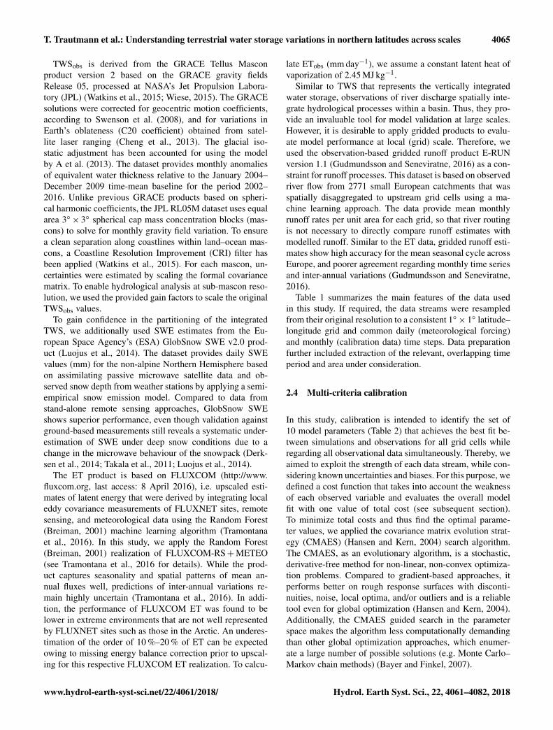
We designed a conceptual hydrological model with low com-plexity and a total number of 10 adjustable parameters. Themodel considers major hydrological fluxes such as snowmelt,sublimation, infiltration, evapotranspiration, and (delayed)runoff and includes water storages in the snowpack, in thesoil, and due to delay in runoff (Fig. 2). It is forced by pre-cipitation (P ), air temperature (T ), and net radiation (Rn)and calculates all hydrological processes on daily time stepsfor individual grid cells. A simple schematic diagram of the

www.hydrol-earth-syst-sci.net/22/4061/2018/ Hydrol. Earth Syst. Sci., 22, 4061–4082, 2018


Figure 2. Schematic structure of the model with calculation ofTWS. Boxes denote the water storages (mm): snow water equiv-alent SWE, soil moisture SM, retained water RW, liquid wa-ter W and total terrestrial water storage TWS. Fluxes are rep-resented by arrows. Red colour identifies forcing data: precipita-tion P (mm day−1), air temperature T (◦C), and net radiation Rn(MJ m−2 day−1); green colour indicates variables constrainedby observations: evapotranspiration ET (mm day−1), runoff Q(mm day−1), SWE (mm), and TWS (mm).

model is shown in Fig. 2, while a detailed description of mod-elled processes is provided in Sect. S1 in the Supplement.

In the first step, precipitation P is partitioned into liq-uid precipitation (rainfall) and snowfall based on a temper-ature threshold of 0◦ C. Accumulating snowfall increases thesnowpack represented by the snow water equivalent (mm),which depletes by sublimation and melt if T exceeds 0 ◦C.We calculate sublimation based on the GLEAM model (Mi-ralles et al., 2011) and apply an extended degree-day ap-proach to estimate snowmelt (Kustas et al., 1994). Since thepresence of snow can be highly variable in one grid cell, wemodel the fractional snow cover (–) following Balsamo etal. (2009), which is used to scale snowmelt and sublimation.

Similar to the WaterGAP model (Döll et al., 2002), incom-ing water from rain and snowmelt is allocated to soil mois-ture (SM) and land runoff (Qs) depending on soil moistureconditions (Bergström, 1991). SM is represented by a one-layer bucket storage that depletes by evapotranspiration (ET).We calculate ET as the minimum of demand-limited poten-tial ET following the Priestley–Taylor formula (Priestley andTaylor, 1972) and supply-limited ET following Teuling etal. (2006).

As land runoff results from an effective soil water rechargeformulation, the calculated runoff is essentially all the waterthat cannot be stored in the soil. Thus, it implicitly containsboth surface and subsurface runoff as well as the percola-tion to deeper water storages such as groundwater, as wellas contributions from surface water bodies. To account forrunoff contributions from slow-varying storages, we calcu-

late runoff from each grid cell (Q) by applying an expo-nential delay function on Qs (Orth et al., 2013). Based onmass balance, we derive the amount of retained land runoff(RW), which implicitly accounts for the effects of severalwater pools that are not explicitly represented in the model(groundwater, lakes, wetlands, and the river storage). Thesum of RW and SM is then taken as the total liquid water stor-age (W ). Frozen soil water is not explicitly included in themodel. Further, the model does not account for lateral flowof water among grid cells and does not consider river routingexplicitly. While the effect of the routing can be significantin large river basins of humid regions (Kim et al., 2009), itis negligible on the spatial scale of a grid cell (as also shownby small influence of the delayed storage component), and atthe temporal scale of monthly aggregated values. To ensurethat the model calibration is not affected by river routing, wedo not compare simulated runoff to measured river dischargeof large basins in our model–data fusion approach.

Finally, the sum of liquid water storage and snow is takenas the modelled terrestrial water storage (TWSmod) of a gridcell for the given time step. Since the delayed runoff contri-bution is minor at the monthly timescale, we, for simplicity,only focus on the contributions of SWE and total W to TWSin this study.

2.3 Input data

As meteorological forcing we used globally available, dailycumulated gridded precipitation sums (mm day−1), aver-age air temperature (◦C), and net radiation (MJ m−2) fromMarch 2000 to December 2014.

Precipitation values originate from the 1◦ daily precipita-tion product version 1.2 of the Global Precipitation Clima-tology Project (GPCP-1DD) (Huffman et al., 2000; Huffmanand Bolvin, 2013), which combines remotely sensed pre-cipitation and observations from gauges. Temperature wasobtained from the CRUNCEP version 6.1 dataset (Viovy,2015), which is a merged product of Climate ResearchUnit (CRU) TS.3.23 observation-based monthly climatol-ogy (1901–2013) (New et al., 2000) and the National Cen-ter for Environmental Prediction (NCEP) 6-hourly reanal-ysis data (1948–2014) (Kalnay et al., 1996). Net radiationis based on radiation fluxes of the SYN1deg Ed3A dataproduct of the Clouds and the Earth’s Radiant Energy Sys-tems (CERES) program of the US National Aeronautics andSpace Administration (NASA) (Wielicki et al., 1996).

Rather than using a single data stream, e.g. discharge mea-surements at the outlet of large continental catchments asused in traditional large-scale hydrological studies, we cal-ibrated the model against multiple observation-based datastreams on the grid scale. The integrated datasets include ter-restrial water storage anomalies (TWSobs) (mm), snow wa-ter equivalent (SWEobs) (mm), evapotranspiration (ETobs)(mm day−1), and gridded runoff estimates for Europe (Qobs)(mm day−1).



TWSobs is derived from the GRACE Tellus Masconproduct version 2 based on the GRACE gravity fieldsRelease 05, processed at NASA’s Jet Propulsion Labora-tory (JPL) (Watkins et al., 2015; Wiese, 2015). The GRACEsolutions were corrected for geocentric motion coefficients,according to Swenson et al. (2008), and for variations inEarth’s oblateness (C20 coefficient) obtained from satel-lite laser ranging (Cheng et al., 2013). The glacial iso-static adjustment has been accounted for using the modelby A et al. (2013). The dataset provides monthly anomaliesof equivalent water thickness relative to the January 2004–December 2009 time-mean baseline for the period 2002–2016. Unlike previous GRACE products based on spheri-cal harmonic coefficients, the JPL RL05M dataset uses equalarea 3◦× 3◦ spherical cap mass concentration blocks (mas-cons) to solve for monthly gravity field variation. To ensurea clean separation along coastlines within land–ocean mas-cons, a Coastline Resolution Improvement (CRI) filter hasbeen applied (Watkins et al., 2015). For each mascon, un-certainties were estimated by scaling the formal covariancematrix. To enable hydrological analysis at sub-mascon reso-lution, we used the provided gain factors to scale the originalTWSobs values.

To gain confidence in the partitioning of the integratedTWS, we additionally used SWE estimates from the Eu-ropean Space Agency’s (ESA) GlobSnow SWE v2.0 prod-uct (Luojus et al., 2014). The dataset provides daily SWEvalues (mm) for the non-alpine Northern Hemisphere basedon assimilating passive microwave satellite data and ob-served snow depth from weather stations by applying a semi-empirical snow emission model. Compared to data fromstand-alone remote sensing approaches, GlobSnow SWEshows superior performance, even though validation againstground-based measurements still reveals a systematic under-estimation of SWE under deep snow conditions due to achange in the microwave behaviour of the snowpack (Derk-sen et al., 2014; Takala et al., 2011; Luojus et al., 2014).

The ET product is based on FLUXCOM (http://www.fluxcom.org, last access: 8 April 2016), i.e. upscaled esti-mates of latent energy that were derived by integrating localeddy covariance measurements of FLUXNET sites, remotesensing, and meteorological data using the Random Forest(Breiman, 2001) machine learning algorithm (Tramontanaet al., 2016). In this study, we apply the Random Forest(Breiman, 2001) realization of FLUXCOM-RS+METEO(see Tramontana et al., 2016 for details). While the prod-uct captures seasonality and spatial patterns of mean an-nual fluxes well, predictions of inter-annual variations re-main highly uncertain (Tramontana et al., 2016). In addi-tion, the performance of FLUXCOM ET was found to belower in extreme environments that are not well representedby FLUXNET sites such as those in the Arctic. An underes-timation of the order of 10 %–20 % of ET can be expectedowing to missing energy balance correction prior to upscal-ing for this respective FLUXCOM ET realization. To calcu-

late ETobs (mm day−1), we assume a constant latent heat ofvaporization of 2.45 MJ kg−1.

Similar to TWS that represents the vertically integratedwater storage, observations of river discharge spatially inte-grate hydrological processes within a basin. Thus, they pro-vide an invaluable tool for model validation at large scales.However, it is desirable to apply gridded products to evalu-ate model performance at local (grid) scale. Therefore, weused the observation-based gridded runoff product E-RUNversion 1.1 (Gudmundsson and Seneviratne, 2016) as a con-straint for runoff processes. This dataset is based on observedriver flow from 2771 small European catchments that wasspatially disaggregated to upstream grid cells using a ma-chine learning approach. The data provide mean monthlyrunoff rates per unit area for each grid, so that river routingis not necessary to directly compare runoff estimates withmodelled runoff. Similar to the ET data, gridded runoff esti-mates show high accuracy for the mean seasonal cycle acrossEurope, and poorer agreement regarding monthly time seriesand inter-annual variations (Gudmundsson and Seneviratne,2016).

Table 1 summarizes the main features of the data usedin this study. If required, the data streams were resampledfrom their original resolution to a consistent 1◦× 1◦ latitude–longitude grid and common daily (meteorological forcing)and monthly (calibration data) time steps. Data preparationfurther included extraction of the relevant, overlapping timeperiod and area under consideration.

2.4 Multi-criteria calibration

In this study, calibration is intended to identify the set of10 model parameters (Table 2) that achieves the best fit be-tween simulations and observations for all grid cells whileregarding all observational data simultaneously. Thereby, weaimed to exploit the strength of each data stream, while con-sidering known uncertainties and biases. For this purpose, wedefined a cost function that takes into account the weaknessof each observed variable and evaluates the overall modelfit with one value of total cost (see subsequent section).To minimize total costs and thus find the optimal parame-ter values, we applied the covariance matrix evolution strat-egy (CMAES) (Hansen and Kern, 2004) search algorithm.The CMAES, as an evolutionary algorithm, is a stochastic,derivative-free method for non-linear, non-convex optimiza-tion problems. Compared to gradient-based approaches, itperforms better on rough response surfaces with disconti-nuities, noise, local optima, and/or outliers and is a reliabletool even for global optimization (Hansen and Kern, 2004).Additionally, the CMAES guided search in the parameterspace makes the algorithm less computationally demandingthan other global optimization approaches, which enumer-ate a large number of possible solutions (e.g. Monte Carlo–Markov chain methods) (Bayer and Finkel, 2007).


http://www.fluxcom.org



Table 1. Overview on data applied for meteorological forcing and multi-criteria calibration and model evaluation (NH: Northern Hemi-sphere).

Variable Dataset Coverage and resolution Reference

Spatial Temporal

Meteorological forcing

P precipitation GPCP 1dd v1.2 1◦× 1◦ daily Huffman et al. (2000),global 1996–present Huffman et al. (2016)

T air CRUNCEP v6.1 0.5◦× 0.5◦ daily Viovy (2015)temperature global 1901–2014

Rn net radiation CERES SYN1deg Ed3A 1◦× 1◦ 3-hourly Wielicki et al. (1996)global Mar 2000–May 2015

Calibration and evaluation

TWS terrestrial GRACE Tellus JPL- 0.5◦× 0.5◦ monthly Watkins et al. (2015),water storage RL05M v2 global 2002–2016 Wiese et al. (2016b)anomalies

SWE snow water GlobSnow v2.0 0.25◦× 0.25◦ daily Luojus et al. (2014)equivalent non-alpine NH 1979–2012

ET evapotranspiration FLUXCOM 0.5◦× 0.5◦ daily Tramontana et al. (2016)global 1982–2013

Q runoff EU-RUN v1.1 0.5◦× 0.5◦ monthly Gudmundsson and Seneviratne (2016)Europe 1950–2015

Table 2. Adjustable model parameters, their meaning, calibration range (theoretical range in brackets), optimized value including estimateduncertainty, and the corresponding equation in S1.

Parameter Description Unit Range Optimized Eq.

(theoretical) value ± uncertainty (%)

Snow

psf scaling factor for snowfall – 0–3 (∞) 0.67 ±1× 10−3 (< 1 %) (S2)snc minimum SWE that ensures complete snow mm 0–500 (∞) 80 ±19 (24 %) (S3)

cover of the gridmt snowmelt factor for T mm K−1 day−1 0–10 2.63 ±0.26 (10 %) (S4)mr snowmelt factor for Rn mm MJ−1 day−1 0–3 0.90 ±0.05 (6 %) (S4)sna sublimation resistance – 0–3 0.44 ±0.01 (3 %) (S5)

Soil

sexp shape parameter of runoff–infiltration curve – 0.1–5 1.46 ±0.02 (2 %) (S12)smax maximum soil water holding capacity mm 10–1000 (0–∞) 515 ±9 (2 %) (S12)eta alpha coefficient in Priestley–Taylor formula – 0–3 1.20 ±0.01 (1 %) (S14)etsup ET sensitivity and/or SM fraction available for ET day−1 0–1 0.02 ±6× 10−5 (< 1 %) (S18)

Runoff

qt recession timescale for land runoff d 0.5 (0)–100 13 ±4 (31 %) (S20)

In order to keep computational demands low and to avoidoverfitting by a very small sample size, we perform cali-bration for a subset of 1000 randomly chosen grid cells.Within this iterative process, the model simulations are car-ried out on daily time steps, while costs are calculated basedon monthly values. Further, each model run includes an ini-tialization based on 10 random years that were selected a pri-ori.

Cost function

To objectively describe the goodness of fit, we defined acost function based on model efficiency (Nash and Sutcliffe,1970), but with explicit consideration of the uncertainty σi ofthe observed data stream as follows:



cost=

n∑i=1

(xobs,i−xmod,i)2

σi

n∑i=1

(xobs,i−xobs)2

σi

, (1)

where xobs,i is the observed data, xobs is the average of xobs,and xmod,i is the modelled data of each space–time point i.Similar to model efficiency, the criterion reflects the over-all fit in terms of variances and biases, yet with an optimalvalue of 0 and a range from 0 to ∞. Costs are calculatedfor each variable separately, considering only grid cells andtime steps with available observations, which vary for thedifferent data streams. Additionally, to overcome the sensi-tivity to outliers arising from data uncertainties or inconsis-tencies, we adopted a 5th-percentile outlier removal criterion(Trischenko, 2002), i.e. the data points with the highest 5 %residuals xobs–xmod were excluded in the cost function.

The costs of each observed variable and its modelled coun-terpart are then added equally to derive a single value of to-tal cost (Eq. 2). Since a perfect simulation would yield a to-tal cost of 0, calibration aims to find the global minimum ofcosttotal.

costtotal = costTWS+ costSWE+ costET+ costQ (2)

As the uncertainty σ of observational data in Eq. (1) isadapted to best reflect the strength of the individual datastream, we preselected the strongest aspect of the data tobe included in the cost function. Owing to the larger uncer-tainties of ETobs and Qobs on inter-annual scales, we onlyemployed the grid’s mean seasonal cycles, while the fullmonthly time series of gridded TWSobs and SWEobs weretaken into account.

As ETobs and Qobs do not explicitly provide uncertaintyestimates, we assume an uncertainty of 10 % and minimumof 0.1 mm, respectively. In order to define σ of TWSobswe utilized the spatially and temporally varying uncertaintyinformation provided with the GRACE data. Additionally,the monthly values of observed and modelled TWS datasetswere translated as anomalies to a common time-mean base-line of their overlapping period 1 January 2002–31 Decem-ber 2012 before calculating the cost for TWS.

For SWE, we applied an absolute uncertainty of 35 mmbased on reported differences to ground measurements (Liuet al., 2014; Luojus et al., 2014). Since GlobSnow SWE satu-rates above approx. 100 mm (Luojus et al., 2014), we do notpenalize model simulations when both SWEobs and SWEmodare larger than 100 mm in order to prevent the propagation ofdata biases to calibrated model parameters.

For maps of the temporal average uncertainties seeSect. S2.

2.5 Evaluation of model performance

Once the parameters were optimized, we applied the modelfor the entire study domain and evaluated its performance

regarding all grid cells (6050) in terms of Pearson correla-tion coefficient r and root mean square error RMSE for eachvariable with observational data. On the one hand, the over-all performance at local scale was assessed by calculating rand RMSE for the monthly time series of each grid individu-ally. On the other hand, the model performance over the en-tire study domain was evaluated by comparing the seasonaland inter-annual dynamics of the regional average. There-fore, we defined inter-annual variation (IAV) as the deviationof the monthly values from the mean seasonal cycle (MSC).As with the calibration, we focused on the common time pe-riod 2002–2012 and considered only the grid cells and timesteps with available observations.

In order to benchmark our model against current state-of-the-art hydrological models, we compared its simula-tions with the multi-model ensemble of the global hy-drological and land surface models of the eartH2Observedataset (Schellekens et al., 2017). This ensemble includesHTESSEL-CaMa (Balsamo et al., 2009), JULES (Best et al.,2011; Clark et al., 2011), LISFLOOD (van der Knijff et al.,2010), ORCHIDEE (Krinner et al., 2005; Ngo-Duc et al.,2007; d’Orgeval et al., 2008), SURFEX-TRIP (Alkama etal., 2010; Decharme et al., 2013), W3RA (van Dijk and War-ren, 2010; van Dijk et al., 2014), WaterGAP3 (Flörke et al.,2013; Döll et al., 2009), PCR-GLOBWB (van Beek et al.,2011; Wada et al., 2014), and SWBM (Orth et al., 2013). Forconsistency, we processed the model estimates in the samemanner as our model simulations to directly compare mod-elled SWE and TWS to observations from GlobSnow andGRACE, respectively. While each model provides simulatedSWE, they vary in the representation of other storage com-ponents. We calculated modelled TWS for each model bysumming up the available water storage components. Thus,the variables contributing to modelled TWS vary betweenthe models, which impedes detailed comparison. Addition-ally, we calculated the multi-model mean of SWE and TWSsimulations.

2.6 Analysis of TWS variations and composition

Finally, the contribution of snow and liquid water to seasonaland inter-annual TWS variability was quantified across spa-tial scales. For this, we ran the model with optimized pa-rameters for the entire study domain from 2000 to 2014 andtranslated simulated storages as anomalies to the time-meanbaseline. As in the model evaluation, the MSC and IAV ofSWEmod, W , and TWSmod anomalies were calculated at lo-cal scale for each grid individually and as spatial averageover all grid cells. To assess storage variability, the variancein the MSC and the IAV of each storage component was com-puted. Assuming negligible covariance of snow and liquidwater (see Sect. S8), their relative contribution to TWS vari-ance was calculated as the contribution ratio CR:



CR=var(W)

var(TWSmod)−

var(SWEmod)

var(TWSmod). (3)

While CR= 0 indicates equal contribution of snow and liq-uid water to TWS variability, positive (negative) values of CRimply that variations of TWSmod mainly result from vari-ations in liquid water (snowpack), with CR=+1 meaningthat all variation is explained by liquid water and CR=−1suggests determination solely by snow.

From Eq. (3) and the assumption that var(W)+var(SWE)= var(TWS), the percentage contribution of liq-uid water storages to the variability of TWS can be inferredas CW:

CW=var(W)

var(TWSmod)=

CR+ 12

. (4)

As this study intends to analyse the effects of storage com-ponents on TWS at different spatial scales (local grid scaleand large (regional) spatial averages), the difference in spa-tial heterogeneities of these components is considered. Somestorage components, e.g. soil moisture anomalies, have muchlarger spatial variability than others. Due to this high small-scale heterogeneity, the effect on larger regional scale mightbe smaller than expected, as different local scale hetero-geneities compensate for each other when the regional av-erages are calculated (Jung et al., 2017). Thus, we assessedthe spatial coherence of simulated patterns of SWE and Wby calculating the proportion of total positive and total neg-ative covariances among grid cells (Eqs. 4 and 5 in Jung etal., 2017). If the sum of positive covariances outweighs thesum of negative covariances, it implies some degree of spa-tial coherence of the anomalies. Spatial coherence of anoma-lies then causes a larger variance in the averaged anomaliescompared to the sum of the variances of individual grid cells.This assessment of spatial coherence of SWE andW anoma-lies allows for understanding different contributions of SWEand W to TWS variability at local scale compared to the re-gional scale.

3 Results and discussion

The following sections present and discuss the results ob-tained with the calibrated model. First, we review the cali-bration approach and the optimized parameter values. Thenthe model is validated with respect to its overall perfor-mance at grid scale, as well as the reproduction of averageseasonal (MSC) and inter-annual (IAV) dynamics. Subse-quently, we assess the driving component of spatially inte-grated TWS variations and the relative contributions of snowand liquid water to TWS variability on local scale. Finally,we summarize the results across spatio-temporal scales.

3.1 Model optimization

Optimization of the model identifies the parameter valueslisted in Table 2 as being most suitable regarding all dataconstraints simultaneously. The CMAES search algorithmconverged after 3272 function evaluations as no further im-provement of coststotal could be achieved, which suggests areliable estimate of the global optimal parameter set. The in-dividual cost terms obtained with default and optimized pa-rameter values are contrasted in Table S1 in the Supplement.Overall, this parameter set obtained for a subset of 1000 ran-dom grids is reasonable with respect to reported “plausible”parameter ranges, with none of them reaching their physi-cally and/or technically defined upper and lower calibrationbounds.

In detail, snowfall is reduced by psf to 67 % of precip-itation occurring at T < 0 ◦C. This reduction agrees withBehrangi et al. (2016), who found that GPCP overestimatedsnowfall over Eurasian high latitudes by about 20 % com-pared to other precipitation products. Similar, overestimationof precipitation undercatch correction in GPCP has been re-ported by Swenson (2010). Taking into account the mismatchin temporal and spatial domains, as well as the experimentaldefinitions, reducing GPCP snowfall in our study by 33 %is roughly consistent with both studies. Therefore, psf al-lows the reduction of inconsistencies between the precipi-tation forcing and the water storages as given by GlobSnowSWE and GRACE TWS.

Further, each grid is assumed to be completely covered bysnow if SWE≥ 80 mm (snc). On the one hand, the snowpackcan be reduced by sublimation, with sna = 0.44 indicatingrelatively high sublimation resistance, compared to a defaultof sna = 0.95 proposed by Miralles et al. (2011). The diver-gence probably results from interaction with snowmelt, asnet radiation also contributes to melt with 0.9 mm MJ−1 (mr)if T exceeds 0 ◦C. On the other hand, melt is mainly inducedby temperature, as the estimated degree-day factor (mt ) is2.63 mm K−1, which is close to typical values of 3 mm K−1

(Müller Schmied et al., 2014; Stacke, 2011). These parameterinteractions underline an equifinality issue between modelledsnowmelt and sublimation due to missing data constraints,resulting in larger parameter uncertainties for sna , mr, andmt . However, for the objective of this study it is not primarilyrelevant whether sublimation- or radiation-induced melt de-creases the snowpack, as the total snow loss amount remainsrelatively unchanged for different parameter combinations.

The maximum soil water holding capacity is set to 515 mmafter calibration, a comparatively high value that is likelyto include storages in surface water bodies such as lakesand wetlands within our study domain. The optimized valueof sexp is 1.46, which suggests a non-linear relationship be-tween soil moisture storage and runoff generation. For thesame amount of incoming water (rainfall and snowmelt), thenon-linear relationship produces a smaller runoff and largerinfiltration than a linear relationship (sexp = 1).



Regarding evapotranspiration, the alpha coefficient (eta) inthe Priestley–Taylor formula is generally taken as 1.26 forwell-watered crops based on experimental observations(Priestley and Taylor, 1972; Eichinger et al., 1996). Thus,the optimized value of 1.20 for eta reflects a plausible value.Further, etsup indicates that 2 % of the available soil moisturecan evaporate per day (including transpiration), which lieswithin the range of site-specific ET sensitivities from 0.001to 0.5 day−1 and is close to the median value (5 %) (Teulinget al., 2006).

Finally, the calibrated recession timescale that delays landrunoff is 13 days (qt ). Compared to much smaller alpinecatchments for which Orth et al. (2013) reported qt of 2days, the longer delay coefficients are reasonable at a spa-tial resolution of 1◦× 1◦ grids, because the elevation gra-dients are much smaller within a large spatial area. At firstglance, 13 days appear to be quite a short effective time pe-riod, as the delay is supposed to comprise contributions frommuch slower depleting reservoirs, such as lakes and deepgroundwater. However, implementing and calibrating a sim-ple groundwater storage, which is recharged with some pro-portion of land runoff and linearly depletes over time, led tosimilar retardation times.

The uncertainty in the optimized parameter vector was es-timated by quantifying each parameter’s standard error as thesquare root of the product between the diagonal elements ofthe parameters’ covariance matrix (calculated from the Ja-cobian matrix) and the sum of residual squares according toOmlin and Reichert (1999) and Draper and Smith (1981).The resulting relative parameter uncertainty is particularlyinstructive for comparing how well individual parameterscould be constrained.

Most parameters were well constrained (Table 2), sug-gesting that our model–data fusion method, fed by multipleobservation streams, succeeded in reducing the initial the-oretical parameter ranges (up to 500 %) to much narrowerranges. Nonetheless, some parameters have a larger uncer-tainty range than others (e.g. qt , snc, mt ), which may high-light a limitation in suitable observations to constrain them,as well as a lower sensitivity of the model results and thecost function used. Further, given that the model only consid-ers the spatial variability of climate, the uncertainty in globalparameters obtained from inversion may reflect the naturalvariations in these parameters that arise from differences inlocal land surface characteristics such as topography or landcover.

We adopted the calibrated parameter values as global con-stants for model simulations over the entire study domain.Even though the globally uniform parameters may not pro-vide perfect simulation for all grids over a large study do-main, this approach represents a compromise between a pri-ori parametrization of the model and its calibration at localor regional (e.g. basin) scale. While local and regional modelcalibration enables good adaption to geographic characteris-tics, it easily leads to overfitting of the model and thus propa-

gates the constraints’ inherent errors and uncertainties in themodelling result. As these uncertainties often vary in space,globally uniform parameter values diminish overfitting un-certainties. In addition, calibration for several independentgrids is computationally demanding and subsequently re-quires a parameter regionalization approach (He et al., 2011).Since such approaches are not commonly accepted (Sood andSmakhtin, 2015; Bierkens et al., 2015), macro-scale modelsmostly apply a priori parameters based on empirical valuesor on expert knowledge, which may yet lead to suboptimalsimulations (Beck et al., 2016; Sood and Smakhtin, 2015).

3.2 Model performance

For model validation, we used the optimized parameter val-ues to simulate hydrological fluxes and states of the 2002–2012 period over the entire study domain and evaluated themodel results against the observation-based data of TWS,SWE, ET, and Q.

In general, all observed patterns are reproduced very well,taking into account the specific data weaknesses. We achievea “near-perfect” correlation of 0.99 and 0.94 for mean sea-sonal variations of ET and Q, respectively. The medianRMSE of mean seasonal ET is 11 and 9.5 mm month−1

for Q, which represent 15 % resp. 17 % of the average ob-served annual amplitude. At the inter-annual scale, though,larger discrepancies exist, which at least partly arise fromlarger uncertainties in ETobs and Qobs (Sect. S4). Thus, weassume high confidence in modelled ET and Q fluxes andsubsequently focus on evaluation of the water storages TWSand SWE.

3.2.1 Performance on local grid scale

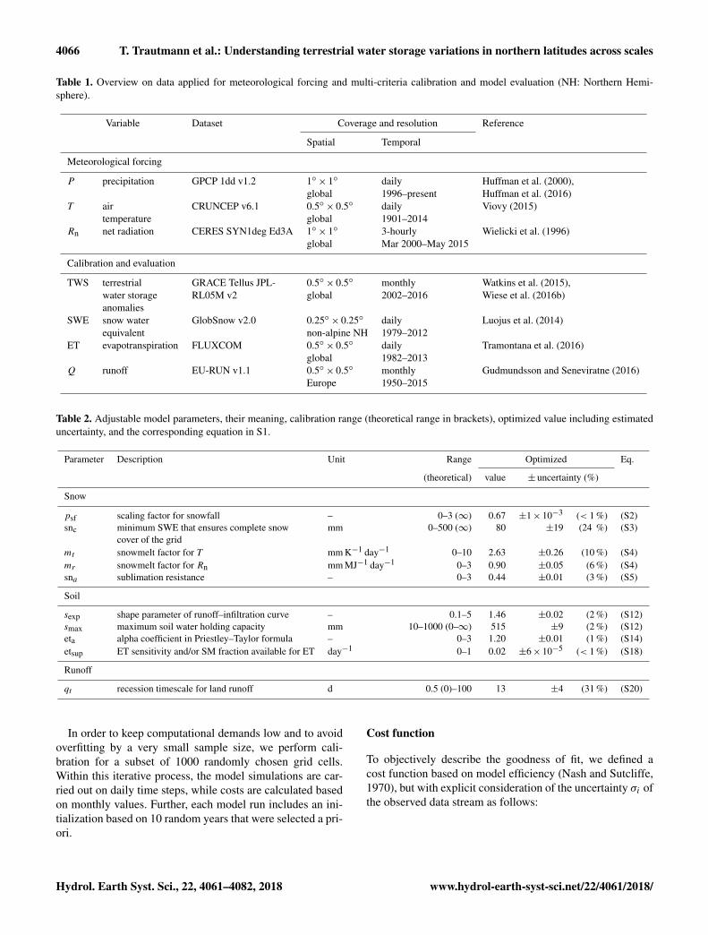
Overall, the model performs well compared to the observa-tions of monthly time series of SWE and TWS (Fig. 3). Morethan half of the grid cells obtain correlation values higherthan 0.74 between SWEobs and SWEmod. In general, the me-dian RMSE is 20 mm, which is smaller than the averageuncertainty of 35 mm in SWEobs. The correlation reducesin lower latitudes where seasonal snow accumulation andthus variability is small. Further, the correlation is also rela-tively weaker in arctic North America and the Rocky Moun-tains, while larger deviations between observed and modelledsnow quantities centre around mountainous and coastal re-gions (e.g. Rocky Mountains, Kamchatka), and regions withthe largest seasonal snow accumulation (Labrador Peninsula,North Siberian Lowland and northern West Siberian Plain).There are several reasons for this relatively poorer perfor-mance. First, the GlobSnow measurements do not covermountainous areas due to the sub-grid variability of snowdepth and high uncertainties in the microwave measurementsin complex alpine terrains (Takala et al., 2011). As the re-sampling and the coarse resolution of each grid in this studycompound a distinct alpine or non-alpine classification, these



Figure 3. Pearson correlation coefficient r (a, c) and root mean square error RMSE (b, d) between monthly values of modelled SWE andGlobSnow SWE (a, b), as well as modelled TWS and GRACE TWS (c, d) for the period 2002–2012 and for each 1◦× 1◦ grid cell of thestudy domain. Values of r are truncated to the range 0–1 (a, c), and values of RMSE to the range 0–100 mm (b, d).

uncertainties leak to the surrounding areas. Second, neitherthe input forcing data nor our model include the sub-gridscale heterogeneity of climate (e.g. precipitation and temper-ature) and hydrological processes, which may be significantin near-mountain or coastal regions. Additionally, the accu-racy of observed large snow accumulation is limited as theradar-retrieval methods tend to saturate at large SWEobs val-ues, which then leads to large RMSE of the model simula-tion.

Similar to SWE, more than half of the grid cells showa strong correlation of 0.71 between TWSobs and TWSmod,which reflects a realistic temporal variation in the model sim-ulation. Compared to SWE, the RMSE of TWS is somewhathigher, yet the median of 43 mm still reflects the range of±22 mm average uncertainty in GRACE TWSobs of the studydomain (Wiese, 2015). However, when comparing GRACE

TWS with model simulations, several aspects have to beconsidered. First, TWSobs as an integrated signal comprisesall water storages, not all of which are (sufficiently) rep-resented in the model structure. Second, although GRACETWS passed through various pre-processing steps, the mod-els that account for postglacial rebound or leakage betweenneighbouring grid cells, for example, introduce their own un-certainties and do not remove the effects completely. Further,with a native resolution of 3◦, uncertainties remain for gridsthat comprise large variability at sub-grid scale and dependon the model used to estimate GRACE scaling factors (Wieseet al., 2016a). Altogether this is reflected in higher RMSEin arctic regions (e.g. surrounding the Hudson Bay), as wellas in heterogeneous coastal and mountainous regions. Addi-tionally, our model shows a weaker performance in subarcticand arctic wetlands, and in central North America and east-



1 2 3 4 5 6 7 8 9 10 11 12Month

0

25

50

75

100

[mm

]

MSC

SWEobs SWEmod consistent SWEmod all

2003 2004 2005 2006 2007 2008 2009 2010 2011 2012Year

-20

10

0

10

20

[mm

]

IAV

1 2 3 4 5 6 7 8 9 10 11 12Month

-80

-40

0

40

80

[mm

]

MSC

TWSobs uncertainty TWSobs monthly value TWSobs TWSmod

2003 2004 2005 2006 2007 2008 2009 2010 2011 2012Year

-20

10

0

10

20

[mm

]

IAV

r = 0.95 r = 0.39

SWE 2002–2012(a)

r = 0.91 r = 0.72

TWS 2002–2012(b)

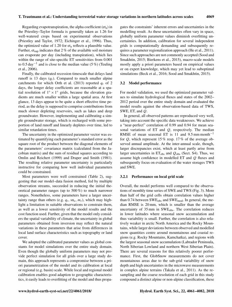
Figure 4. Spatially averaged mean seasonal cycle (MSC) of the period 2002–2012 as well as inter-annual variability (IAV, difference betweenmonthly values and the MSC) for (a) SWE and (b) TWS. In (a), SWEmod consistent refers to modelled SWE considering only data pointswith available SWEobs, while SWEmod all incorporates all time steps for all grids of the study domain. Correlation r is calculated only forconsistent data points. In (b) IAV, TWSobs monthly value shows the original IAV of individual TWSobs months, while TWSobs and TWSmodare smoothed using a 3-month average moving window filter. Correlation r refers to the smoothed values. For the MSC in (b) no smoothingis applied.

ern Eurasia. The latter are both relatively dry regions that arerather dominated by inter-annual TWS variations (Humphreyet al., 2016). Discrepancies between TWSobs and TWSmodthus relate to a low signal-to-noise ratio in TWSobs due tosmall seasonal TWS variations. However, the anthropogenicinfluence for irrigational withdrawal is very large in these re-gions, yet such processes are not considered in our model.We also lack explicit surface water storages (including wet-land dynamics), which may be the reason for poorer perfor-mance, especially in North American wetland regions.

3.2.2 Performance of the spatially integratedsimulations

Since the aim of this study is to analyse the composition ofTWS across temporal scales, we additionally evaluated aver-age (spatially integrated) MSC and IAV of SWE and TWS(Fig. 4). While the mean seasonal variations of both observa-tional data streams are relatively robust and have been usedfor model evaluation before (Alkama et al., 2010; Döll et

al., 2014; Schellekens et al., 2017; Zhang et al., 2017), theirinter-annual variations are more uncertain and contain con-siderable noise. This clearly reduces the information contentin the observational data, so that we evaluate the IAV in morequalitative terms.

As with the comparison at grid scale, the spatially av-eraged SWEmod compares well to SWEobs, with a corre-lation of 0.95 suggesting a good reproduction of seasonalsnow accumulation and ablation processes (Fig. 4a). Owingto the high uncertainty of SWEobs peaks due to signal sat-uration, the higher amplitude of SWEmod seems reasonable.Although inter-annual variations are not as well representedas the MSC, general tendencies, e.g. increasing/decreasingpositive/negative anomalies, coincide.

Similar to SWE, the spatial average of TWS shows highcorrelation of 0.91 for seasonal variations, with positiveanomalies from December to May–June and negative anoma-lies during summer and autumn months (Fig. 4b). Eventhough the modelled amplitude is slightly larger than the ob-served one, it stays within the uncertainty range of TWSobs



for most months, suggesting reliable simulations. However,TWSmod precedes TWSobs on average by 1 month, reach-ing the maximum in March instead of April, and the mini-mum in August instead of September. A similar phase shiftof 1 month between GRACE TWS and modelled TWS hasbeen reported by several state-of-the-art global models (Döllet al., 2014; Schellekens et al., 2017). It should be notedthat some areas such as eastern North America, Kamchatka,Scandinavia, and western Europe do not show phase differ-ences, while the lag in south-eastern Eurasia is even larger,as already suggested by lower overall correlation (Fig. S5).In general, the disagreement in timing is attributed to thelack of sufficient water storages and the delay mechanismwithin the model, so that the modelled system reacts too fast(Schellekens et al., 2017; Döll et al., 2014; Schmidt et al.,2008). Thus, we implemented model variants with an ex-plicit groundwater storage to delay depletion of TWS, withspatially varying soil properties to better represent hetero-geneous infiltration and runoff rates, as well as a variantthat applied a more sophisticated approach to calculate snowdynamics based on energy balance. Despite the efforts, weachieved no improvement in terms of reducing the phaseshift. Therefore, the question arose as to whether it is not pri-marily the model formulation that prevents correction of thetemporal delay, but rather the combination of forcing dataand observational constraints. To further preclude possibleerrors due to such data inconsistencies, e.g. between GRACETWS and GlobSnow SWE, we excluded GlobSnow SWEdata from calibration. Although this could slightly improvethe agreement of TWS MSC, it led to unrealistic behaviourof snow dynamics, and thus did not offer any advantages.Besides, we found no major differences in the magnitude orspatial distribution of the phase shift resulting from the pre-cipitation forcing (GPCP vs. WFDEI) or compared to otherGRACE solutions (Sect. S6). Further, the lag in TWS sim-ulation can occur due to several mechanisms and processesthat are not yet considered in the current model structure,such as lateral flow and surface storages (wetland and lakes),vegetation processes, glacier melt, and human influence withdams and reservoirs. However, we do not observe a generalor systematic relationship with either elevation, land covertype, soil properties, or the occurrence of lakes and wetlands.There is a tendency that larger negative lags occur more fre-quently in regions with sporadic permafrost, but the ranges ofpermafrost fractions are large for both short and long lags inTWS, suggesting a complex interaction between permafrostextent and its effect on lag in seasonal TWS dynamics. Fi-nally, potential biases in the timing of ET due to snow coverand/or vegetation processes may also affect the timing ofthe depletion of SM and TWS. Additionally, high uncertain-ties of the precipitation forcing and GlobSnow SWE prod-uct in (near-)mountain regions, as well as leakage errors inthe GRACE signal influence the accuracy of both TWSobsand TWSmod. Although these shortcomings should be keptin mind, we assumed that they do not significantly affect our

results regarding to the relative contributions of snow andliquid water to TWS.

In terms of inter-annual variations, the variance in monthlyTWSobs values is highly underestimated by modelled TWS,which on the one hand relates to noise within the GRACEsignal, but on the other hand may again reflect missing pro-cess representation in the model. To reduce the noise, weapplied a 3-month moving-average filter on the monthlytime series. The smoothed time series then shows fairlygood agreement of inter-annual dynamics, with correlationr = 0.68 (Fig. 4b, solid lines). Only the amplitude of thelarge negative anomaly in 2003 is not captured by the model.While the spatial pattern of this negative TWS anomaly canbe simulated, the forcing data do not show large anomaliesin 2003, so that the model fails to reproduce the magnitudeof observed TWS, especially in North America. Issues withthe precipitation forcing are further suggested by a negativeSWE anomaly of on average 5 mm (see Fig. 4a), indicatedin the GlobSnow data, that is not captured by the model, ei-ther. The reason why this snow anomaly is not captured bythe forcing remains unclear at this point – it persists whenusing the WFDEI forcing dataset. Besides, the agreementbetween GRACE and modelled TWS IAV gets substantiallybetter when isolating inter-annual variations by removing thetrends in both TWS time series (increase in correlation rfrom to 0.77). This suggests that the trend in GRACE TWSis to some extent either subject to observational issues or rep-resents a process that is not captured by the model.

3.2.3 Comparison with the eartH2Observe modelensemble

Compared to the model ensemble of the eartH2Observedataset, we achieve an equally good or better performance forthe spatially integrated SWE and TWS on both MSC and IAVscales (Figs. 5 and S6). Besides, the majority of the modelensemble obtains similar spatial patterns of performance cri-teria for SWE as well as for TWS (not shown).

The average observed MSC of SWE is captured with a cor-relation in the range of 0.79 (PCR-GLOBWB) to 0.99 (OR-CHIDEE), whereby only ORCHIDEE shows a better corre-lation than our model (r = 0.95). However, modelled snowaccumulation exceeds that of SWEobs for the majority of themodels, which is also reflected in higher RMSE (Figs. S6–S8). On IAV scales, the correlation is lower in general, yetagain we obtain a better fit (r = 0.39) than the model en-semble (r = 0.12 – ORCHIDEE – to 0.28 – LISFLOOD).However, it remains uncertain whether the discrepancies be-tween SWEobs and SWEmod represent model deficiencies orevolve from issues related to the GlobSnow SWE retrieval(Schellekens et al., 2017).

Regarding average seasonal TWS variations, our modelperforms as well as the model ensemble (r = 0.91), withthe range of the eartH2Observe ensemble spanning fromr = 0.83 (ORCHIDEE) to r = 1.00 (PCR-GLOBWB). The



Comparison of Pearson correlation

MSC IAV MSC IAV0.1

0.2

0.3

0.4

0.5

0.6

0.7

0.8

0.9

1

eartH2Observe model ensembleModel meanThis study

(a) SWE (b) TWS

Figure 5. Pearson correlation for the spatially integrated SWE (a)and TWS (b) achieved by this study compared to the model ensem-ble of the eartH2Observe dataset across temporal scales. In eachbox, the edges represent the 25 % and 75 % percentiles of the modelensemble, while the solid black line marks the performance of theensemble mean.

amplitudes in the MSC of TWSmod (95 to 156 mm) arecomparable to the observed amplitude of 118 mm, exceptfor SWBM, whose amplitude is twice as large as that ofTWSobs. This discrepancy is reflected in relatively highRMSE values for SWBM (Fig. S8). The model ensemble pre-cedes observed seasonal TWS variations by 1 to 1.4 months,similar to our estimates of TWSmod (−1.1 month). OnlyPCR-GLOBWB, with a higher correlation than other mod-els, shows a smaller average lag of less than 1 month(−0.3 months). This minor difference results from balanc-ing out the preceding and succeeding of TWSmod in differentregions over the study domain. Additionally, Schellekens etal. (2017) found that PCR-GLOBWB shows unrealistic snowaccumulation over time in Europe and boreal North Amer-ica. Except for PCR-GLOBWB, the majority of the modelsobtain comparable spatial pattern of preceding TWS, withsmall differences at regional scales. Even though the differ-ence in the MSC is commonly attributed to the lack or inad-equate size and number of water storages (Kim et al., 2009),a relationship between model performance and model com-plexity is not obvious. Relatively complex models, such asHTESSEL, SURFEX, and JULES, show similar phase dif-ferences to simpler models, such as SWBM and our model(−1.0 and −1.1 months, respectively). Since Schellekens etal. (2017) found the largest phase differences in cold regions,they postulate the implementation of processes associatedwith snow as an important factor for this phase lag. In thiscontext, constraining the model with snow observations as

done in our study should increase confidence in the repre-sentation of snow processes. Nevertheless, we obtain a simi-lar phase difference, which points to the importance of otherhydrological processes and storages even in snow-affectedregions.

Although our modelling framework assimilates informa-tion from more data streams compared to the model sim-ulations in the EartH2Observe ensemble, e.g. GRACE andGlobSnow data, we only used a subset of 1000 randomgrid cells to constrain the model parameters. Despite this,our model performs better than the EartH2Observe ensem-ble over the whole domain (6050 grids). This improvementin model performance is also consistent among several mod-elled variables and not limited to storage components only.This suggests that remote sensing data, with larger spatialcoverage than site measurements, have large potential to im-prove hydrological simulations over a large domain. In ad-dition, remote sensing data also hold potential beyond theiruse as an observational constraint and can provide informa-tion on identifying and formulating functional relationshipsacross several spatial and temporal scales, which should beaddressed in future efforts.

All in all, we conclude that our simple model with a globaluniform parameter set achieves considerably good perfor-mance regarding observed patterns, especially compared towell-established, more complex models, and with respect toits simplicity and given uncertainties of forcing and calibra-tion data. Thus, we found the model results to be suitable toanalyse the composition of TWS across spatial and temporalscales.

3.3 TWS variation and composition

3.3.1 Spatially integrated

To assess the average composition of seasonal and inter-annual TWS variations, we spatially integrated mod-elled TWS anomalies as well as modelled anomalies ofsnow (SWE) and liquid water storages (W ) across all gridsof the study domain (Fig. 6).

Regarding the MSC, all water storages show a clear sea-sonal pattern. The maximum TWSmod in March coincideswith the maximum in SWEmod. On the contrary, W re-mains nearly constant throughout the winter, related to thelack of evapotranspiration losses and missing infiltrationdue to prevailing solid precipitation. Starting from March,snowmelt decreases SWEmod, and thus TWSmod, progres-sively. Thereby TWSmod declines with some delay, as posi-tiveW anomalies in April and May suggest buffering of meltwater in the soil and on the surface before being transferredto runoff or evapotranspirated. During the summer months,snow is absent, while W decreases due to higher summer-time evapotranspiration, and preceding runoff of temporar-ily stored water. With W and SWEmod being at their mini-mum in August–September, TWSmod reaches its minimum,



1 2 3 4 5 6 7 8 9 10 11 12Month

-80

-40

0

40

80[m

m]

MSC

TWSmod SWEmod Wmod

2001 2003 2005 2007 2009 2011 2013Year

-20

10

0

10

20

[mm

]

IAVTWS composition 2000–2014

Figure 6. Spatially averaged mean seasonal cycle (MSC) of the period 2000–2014 as well as inter-annual variability (IAV, difference betweenmonthly values and the MSC) for modelled TWS, SWE, and W anomalies to the time-mean of 2000–2014.

too, before starting to increase again in September–October.This rise relates to dropping evapotranspiration rates in com-bination with more precipitation input (increasing W ) andbeginning snow accumulation (increasing SWEmod). Despitethe interplay of SWEmod and W on seasonal variations ofthe integrated TWSmod, the amplitude of W (62 mm) isconsiderably lower than the one of SWEmod (92 mm) andTWSmod (144 mm). Thus, the seasonal accumulation of snowlargely determines the magnitude of TWSmod. Additionally,W anomalies at least partly result from snowmelt, whereasliquid water does not influence the snowpack. Thus, we con-clude that average seasonal TWS variations in northern mid-to high latitudes are mainly driven by annual snow accumu-lation and ablation processes. The CR (Eq. 3) based on thespatially averaged MSC underlines this, as CR=−0.26 in-dicates that variations in SWEmod explain 63 % of seasonalTWSmod variability (CW= 37 %). This agrees with previousfindings of Güntner et al. (2007), who found that SWE con-tributes to 68 % of seasonal TWS variations in cold regionsusing the WaterGAP model.

On IAV scales, the pattern seems less homogeneous(Fig. 6). In contrast to the MSC, CR= 0.25 suggests a largerinfluence from liquid water anomalies (CW= 62.5 %) thansnow anomalies on inter-annual TWS variations. Thereby,we found the main contributor to TWSmod anomalies be-ing dependent on the phase of previous precipitation anoma-lies, in that they define whether snowfall anomalies lead toanomalies in the SWEmod, or whether rain anomalies directlyinfluence W . Additionally, precipitation input shows largerinter-annual variability than evapotranspiration or runofflosses, and thus dominates the change in water storages onIAV scales (not shown). Large TWSmod anomalies, such asin 2005, 2010, and 2012, follow anomalies in wintertime pre-cipitation and go along with anomalies in SWEmod (Fig. 6).On the contrary, summertime anomalies related toW are usu-ally less pronounced in their magnitude (e.g. 2003, 2006).We attribute this to the accumulating effects of snow stor-

age anomalies over the cold period, as they integrate allanomalies of previous cold months while the impact ofevapotranspiration and runoff is reduced. Accordingly, thelargest TWSmod anomalies are obtained in early spring be-fore snowmelt starts and when snow accumulation is high-est. Nevertheless, since W is influenced by the quantityof snowmelt, anomalies in SWEmod implicate subsequentchanges in W . Additionally, snowpack anomalies are elim-inated each summer, while W anomalies dominate the sum-mer. As a result, W anomalies in any case affect TWSmodvariability on IAV scales when analysing the spatial averagecomposition.

Besides, Güntner et al. (2007) demonstrated a shift fromshort-term storages with high seasonality such as SWE onMSC scales towards storages with longer delay times onIAV scales. Although modelled W mainly represents soilmoisture, it implicitly includes surface water and groundwa-ter storages. Thus, its contribution of CW= 62.5 % to inter-annual TWS variations is roughly comparable to 55 % con-tribution from soil moisture (27 %) and surface water (28 %)in cold regions, found by Güntner et al. (2007). Despite this,the relatively large influence of surface water bodies shownby Güntner et al. (2007) suggests that the lack of explicitsurface water storages in this study may contribute to the re-maining discrepancies with GRACE and the lower magni-tude of modelled inter-annual TWS variability compared toGRACE estimates.

3.3.2 Local grid scale

Based on CR (Eq. 3), Fig. 7 shows the relative contribu-tion of SWEmod and W variances to total TWSmod variabil-ity on MSC and IAV timescales for each grid. Thereby, bluecolours represent prevailing SWEmod variations as indicatedby CR< 0, while red colours show the dominance of varia-tions in W (CR> 0).



Accordingly, variations in the MSC of TWSmod are mainlyinfluenced by snow in northern regions, with the meanCR=−0.30 indicating that on average 65 % of seasonalTWSmod variability can be explained by SWEmod (CW=35 %) (Fig. 7a). The contribution of the variation in liquidwater in general increases southwards and prevails seasonalTWSmod variability south of approximately 50◦ latitude. Anexception is Europe, where the influence of W reaches up to60◦ latitude, and where the transition to snow-dominated re-gions is more gradual. Since the calculated variations in RWare low, the majority of modelled W represents variabilityin SM.

This obtained pattern confirms earlier studies that showedthe dominance of snow in northern latitudes in North Amer-ica (Rangelova et al., 2007), and prevailing soil moisture dy-namics further south, e.g. in the Mississippi basin (Ngo-Ducet al., 2007; Güntner et al., 2007). Besides, the north extentof dominating W reflects the temperature gradient in NorthAmerica and Eurasia. Comparison with average annual tem-perature suggests that for T > 10 ◦C variability of W domi-nates, while for T < 0 ◦C SWEmod dynamics prevail. This isplausible, as temperature determines annual snow accumu-lation, and the relative contribution of liquid water increasesin the absence of snow. Yet, it further highlights the depen-dency on the temperature dataset used, especially in a modelthat calculates snowfall and snowmelt based on temperaturethresholds as ours does.

Opposed to the MSC, the variability of W dominatesTWSmod variations on IAV scales in the entire study domain,as is clearly indicated by average CR= 0.63 (Fig. 7b). Inter-annual variations of SWEmod seem to be relevant only in re-gions that receive the highest annual snow amounts, such asthe Canadian Arctic Archipelago, the northern west coast ofNorth America, north-eastern Siberia, and the northern WestSiberian Plain. Due to a prolonged cold period there, the timespan with rainfall and evapotranspiration is short, decreasingthe occurrence of potential variability in W . However, evenin these regions the influence of SWEmod is low compared tothe MSC. This reduced importance of snow on inter-annualscales again agrees with the findings of Güntner et al. (2007).

Apart from that, and since we already showed a linkbetween average TWSmod IAV and previous precipitationanomalies, and as precipitation represents the main modelforcing data, we investigated the relative contribution of rain-fall and snowfall to inter-annual variability of total precip-itation (Fig. 8). Similar to the composition of TWSmod onlocal scale, rain anomalies prevail for most of the grid cells(mean CR= 0.68). This is consistent when snowfall is notscaled by psf and thus suggests that the greater contributionof W to inter-annual variations of TWSmod on local scalerelates to highly variable (liquid) summertime precipitationevents. On the contrary, monthly snowfall seems less vari-able between years, resulting in less pronounced variationsin SWEmod compared to W . Exceptions are regions of highmaximum SWEmod, which accordingly show a considerable

relative contribution of snow to the inter-annual TWSmodvariability.

3.3.3 Comparison of different scales

Figure 9 summarizes the above-presented contributions toTWSmod variability across spatial and temporal scales. Asexplained in the previous sections, we obtained two scale-dependent differences in the relative contribution to TWSmodvariability: (1) in general between temporal scales, and(2) for inter-annual variability between spatial scales.

Regarding (1), Fig. 9 emphasizes again that seasonal vari-ations of TWSmod are mostly determined by seasonal snowdynamics, while on inter-annual scales TWSmod variabilitymainly originates from variations in liquid water. As previ-ously stated, determination by SWEmod dynamics on MSCscales relates to the pronounced magnitude of seasonal snowvariations in northern mid- to high latitudes. In comparison,average monthly changes in W were found to be minor andadditionally influenced by snow ablation. Thereby, the spa-tially integrated CR (black star) roughly agrees with the av-erage of local contributions (dashed line).

Concerning IAV scales, we found that the determination ofTWSmod variability byW relates to larger inter-annual varia-tions in liquid precipitation compared to snowfall. However,considerable differences between spatial scales exist (Fig. 9).Opposed to the MSC, the spatially integrated CR (black star)for IAV is not within the interquartile range of local CR.This indicates a relatively larger effect of SWEmod variationswhen looking on the spatially integrated values compared tolocal values. Liquid water storages are highly heterogeneousin space, mainly due to heterogeneous rainfall anomalies. Onthe contrary, snow variability is affected by fewer factors,and mainly regulated by a range of temperature values thatcontrol freezing and melting. Temperature anomalies in turnshow sizeable spatial coherence across large areas. To assessthe spatial coherence of W compared to SWEmod, we calcu-lated the proportion of total positive and total negative co-variances among grid cells (Fig. 10).

For inter-annual variations of SWEmod, the sum of pos-itive covariances prevails (Fig. 10a), whereas positive andnegative values are more in balance for W (Fig. 10b). Thissuggests that SWEmod anomalies are more spatially coher-ent than anomalies of W . Thus, when spatially averaging,the more homogeneous snow anomaly patterns gain impor-tance. On the contrary, opposed anomalies of W compensatefor each other more strongly. This leads to a relatively largerinfluence of SWEmod to the spatially integrated inter-annualTWSmod variability compared to when analysing the localgrid scale. Since positive covariation clearly dominates fortemperature anomalies, the spatial coherence of SWEmod re-lates to their homogeneous patterns (Fig. 10c). Similar toW ,positive covariances only slightly outweigh year-to-year vari-ations in rainfall (Fig. 10d). The same is true for snowfall(not shown). Therefore, the spatial coherence of SWEmod



Figure 7. Relative contribution based on CR (Eq. 3) of modelled snow (SWE) and liquid water (W ) storage anomalies to (a) mean seasonalvariations from 2000 to 2014 of modelled TWS anomalies, and (b) inter-annual variations of modelled TWS anomalies for each grid cell ofthe study domain.

Figure 8. Relative contribution based on CR (Eq. 3) of modelledsnowfall and rainfall to total precipitation (P ) anomalies on inter-annual (IAV) scales for each grid cell of the study domain.

anomalies is less pronounced than for temperature, as snowis additionally influenced by snowfall anomalies. RegardingW anomalies, this indicates that the spatial heterogeneity inour model, which misses explicit information on soils, topog-raphy, etc., mainly results from inhomogeneous patterns inrainfall anomalies. Thereby, the slightly more balanced posi-tive and negative covariations forW compared to rainfall canbe ascribed to the additional impact of primarily radiation-driven evapotranspiration to SM.

In order to ensure that these results are not artificiallycaused by the forcing data, we did the same analysis runningthe model with rain and snowfall estimates of the WFDEI

Contribution to TWS variability

SWE

50:50

W

Local scale Spatially aggregated

CR

[-]

MSC IAV

-1.0

-0.5

0

0.5

1.0

Figure 9. Relative contribution of snow (SWE) and liquid wa-ter (W ) to TWS variability on different spatial (local grid scale, spa-tially integrated) and temporal (mean seasonal MSC, inter-annualIAV) scales based on CR (Eq. 3). The box plots represent the distri-bution of grid cell CR, with the dashed line marking the correspond-ing average. The star represents the CR calculated for the spatiallyintegrated values.

product (Weedon et al., 2014). Since we observed the samepatterns, we assume our findings to be robust (Sect. S7.1).

3.4 Limitations of the approach

Although the model of this study reproduces observed hy-drological patterns well and achieves comparable results tostate-of-the-art models, its low complexity and the applied



SWE anomalies

34 %

66 %

W anomalies

44 %

56 %

Temperature21 %

79 %

Rainfall

41 %

59 %

(a) (b)

(c) (d)

Figure 10. Proportion of total positive (grey) and negative (or-ange) covariances among grid cells for inter-annual variations of(a) snow (SWE), (b) liquid water storages (W ), (c) temperature,and (d) rainfall.

calibration approach are associated with limitations in termsof process understanding and predictive power.

First of all, the simple structure only allows inferenceson represented processes, which likely include effects offluxes and storages not considered explicitly. For example,the model does not resolve individual liquid water storagessuch as deep groundwater and surface water explicitly. Asdiscussed previously, our delayed land runoff comprises var-ious (intermediate) storages and delay times, and thus can-not be associated with one distinct storage component. Eventhough soil moisture is distinguished from these slowly vary-ing reservoirs, its quantity and pattern have not been directlyvalidated. Future research is required to increase confidenceby including remote-sensing-based data of soil moisture incalibration and/or validation. However, these satellite datastill have limited value as the microwave signals can onlycapture moisture in the upper 5 cm of soil and do not pro-vide estimates under snow cover and dense vegetation (Döllet al., 2015; Lettenmaier et al., 2015). Therefore, a multi-layer soil scheme is needed to compare model outputs tosatellite-derived soil moisture estimates, as was successfullydemonstrated by Albergel et al. (2017) for example.

Further, the model does not include any human-inducedchanges in water storages, which yet contribute to observedTWS variability in many regions (Döll et al., 2015; Rodell etal., 2015). Other simplified or ignored hydrological processesinclude the coincident occurrence of rain and snowfall, liquidwater capacity of snow, interception, freeze–thaw dynamicswithin the soil, capillary rise, and other surface-groundwaterinteractions, the effect of vegetation or other surface prop-erties, and lateral flow from one grid cell to another. In thedownstream areas of large basins especially, the latter repre-

sents a potential input that may significantly affect total TWS(Kim et al., 2009) and thus may contribute to the discrepancybetween TWSobs and TWSmod in some regions. Besides, themodel does not account for spatial variability of topographyand land surface characteristics.

With regards to model parameters, we apply a global uni-form parameter set and do not regionalize the parametersaccording to spatially distributed physio-geographical char-acteristics. In contrast, most macro-scale hydrological mod-els include spatially distributed soil properties to define pa-rameters related to infiltration, soil water holding capacity,and percolation, as well as vegetation types to assess theeffects of different plant functional types on evapotranspi-ration and canopy storage (Sood and Smakhtin, 2015). Ourmodel only implicitly considers the effects of vegetation, forexample on ET, but not its spatial variability, as the asso-ciated impacts are included in the observational constraint.Spatial variability of model parameters might affect the rel-ative contributions of different storage components to TWSvariability at different spatial scales. However, the compar-ison with eartH2Observe models, which generally involvespatial heterogeneity in model parameters, suggests that themain conclusions remain unchanged. Additionally, we wantto highlight that the spatial distribution of model parametersdepends on assumptions and some degree of simplificationas well and thus does not necessarily improve model perfor-mance compared to a global uniform parameter set obtainedfrom multiple observational data. Further, as we encounteredissues with parameter equifinality, especially between mod-elled snowmelt and sublimation, future efforts should includea stronger utilization of runoff data in the calibration andvalidation process. This would help to better constrain wa-ter fluxes to the atmosphere and liquid water fluxes, whichcan contribute to the runoff.

Finally, though the implemented cost function explicitlyaccounts for the uncertainty of the calibration data and addi-tional uncertainties of other input data, their processing andcharacteristics remain partly unaddressed.

4 Conclusion

In this study, we assessed the relative contributions of snow-pack versus soil and retained water variations to the vari-ability of total terrestrial water storage (TWS) for northernmid- to high latitudes. To do so, we constrained a parsi-monious hydrological model with multi-criteria calibrationagainst multiple Earth observation data streams, includingTWS from GRACE satellites and snowpack estimates fromGlobSnow. The optimized model showed considerably goodagreement with observed patterns of hydrological fluxes andstates, and was found to perform comparably to or betterthan simulations from state-of-the-art macro-scale hydrolog-ical models. This underlines the potential of simple hydro-logical models tied to observational data streams as powerful



tools to diagnose and understand large-scale water cycle pat-terns. Further, it highlights the benefits of considering mul-tiple complementary data constraints to overcome their indi-vidual shortcomings.

Consistent with previous studies, we found that seasonalTWS variations are dominated by the development of snow-packs during winter months in most places of the mid- tohigh northern latitudes. In contrast to this seasonal pattern,our study reveals that not snow but anomalies in liquid wa-ter storages, mainly comprising soil moisture, drive inter-annual TWS variations in almost the entire spatial domain.This counter-intuitive pattern was found to relate to largerrainfall anomalies compared to snowfall anomalies.

Apart from the timescale-dependent dominant controlson TWS variations, we additionally observed different be-haviour across spatial scales. In terms of seasonal variations,the spatially integrated contribution reflects the average ofthe spatial domain. However, and more interestingly, the rel-ative contribution of snowpack variations to total TWS inter-annual anomalies appears to be larger when spatially inte-grated than at local scale. We found this pattern results fromstronger spatial coherence of snowpack anomalies comparedto anomalies in other storages, such that the latter cancelout more strongly than the former when calculating an av-erage across large spatial domains. The stronger spatial co-herence of snowpack anomalies seems to be driven by thenature of spatially coherent temperature anomalies that de-termine snow accumulation and melt. These findings implythat patterns from large-scale integrated signals should notbe associated with locally operating processes, since spatialcovariations of climatic variables can confound the picture.

Overall, our study underlines the benefits of GRACE TWSas a model constraint, and moreover, stresses the importanceof temporal and spatial scale when assessing the determi-nants of TWS variability. Clearly, insights obtained at onescale cannot be transferred to another, as is often (uninten-tionally) done. Hence, TWS variations in northern latitudesseem to be not merely subject to snow variability, but ratherare driven by soil moisture on inter-annual scales – whichmay be of considerable importance when assessing long-term water availability in the context of climate changes.

Data availability. The hydrological model and all simulation re-sults from this study can be obtained from the corresponding au-thor on request. Due to the large size and quantity of the data,along with potentially few users of the “same” simulation resultsin the foreseeable future, it is not hosted on any public platform.The forcing and calibration data is publicly available as specifiedwith the corresponding citation. For ETobs, the subset of FLUX-COM (http://www.fluxcom.org, Jung and FLUXCOM team, 2016)data used in this study is available from the data portal of the MaxPlanck Institute for Biogeochemistry (https://www.bgc-jena.mpg.de/geodb/projects/Home.php) after registration.

The Supplement related to this article is availableonline at https://doi.org/10.5194/hess-22-4061-2018-supplement.

Author contributions. TT, SK, and MJ designed the research in ex-tensive collaboration with NC, AE, and MF. CN processed and inte-grated runoff estimates from E-RUN in model calibration. NC con-tributed to parameter estimation and uncertainty analysis. TT con-ducted the analysis. All co-authors contributed to the preparation ofthe paper.

Competing interests. The authors declare that they have no conflictof interest.

Special issue statement. This article is part of the special issue “In-tegration of Earth observations and models for global water re-source assessment”. It does not belong to a conference.

Acknowledgements. This research was carried out within theinitiative for the development of the SINDBAD (Strategies toIntegrate Data and Biogeochemical models) framework.

The article processing charges for this open-accesspublication were covered by the Max Planck Society.

Edited by: Jean-Christophe CalvetReviewed by: Vincent Humphrey and one anonymous referee

References

A, G., Wahr, J., and Zhong, S.: Computations of the vis-coelastic response of a 3-D compressible Earth to sur-face loading: an application to Glacial Isostatic Adjustmentin Antarctica and Canada, Geophys. J. Int., 192, 557–572,https://doi.org/10.1093/gji/ggs030, 2013.

Albergel, C., Munier, S., Leroux, D. J., Dewaele, H., Fairbairn, D.,Barbu, A. L., Gelati, E., Dorigo, W., Faroux, S., Meurey, C.,Le Moigne, P., Decharme, B., Mahfouf, J.-F., and Calvet, J.-C.:Sequential assimilation of satellite-derived vegetation and soilmoisture products using SURFEX_v8.0: LDAS-Monde assess-ment over the Euro-Mediterranean area, Geosci. Model Dev., 10,3889–3912, https://doi.org/10.5194/gmd-10-3889-2017, 2017.

Alkama, R., Decharme, B., Douville, H., Becker, M., Cazenave, A.,Sheffield, J., Voldoire, A., Tyteca, S., and Le Moigne, P.: GlobalEvaluation of the ISBA-TRIP Continental Hydrological System.Part I: Comparison to GRACE Terrestrial Water Storage Esti-mates and In Situ River Discharges, J. Hydrometeorol., 11, 583–600, https://doi.org/10.1175/2010jhm1211.1, 2010.

AMAP: Snow, Water, Ice and Permafrost in the Arctic(SWIPA) 2017, Arctic Monitoring and Assessment Pro-gramme (AMAP), Oslo, Norway, xiv+269, 2017.

Balsamo, G., Beljaars, A., Scipal, K., Viterbo, P., van denHurk, B., Hirschi, M., and Betts, A. K.: A Revised Hy-



https://www.bgc-jena.mpg.de/geodb/projects/Home.php


https://doi.org/10.5194/hess-22-4061-2018-supplement

https://doi.org/10.5194/hess-22-4061-2018-supplement

https://doi.org/10.1093/gji/ggs030

https://doi.org/10.5194/gmd-10-3889-2017

https://doi.org/10.1175/2010jhm1211.1


drology for the ECMWF Model: Verification from FieldSite to Terrestrial Water Storage and Impact in the In-tegrated Forecast System, J. Hydrometeorol., 10, 623–643,https://doi.org/10.1175/2008jhm1068.1, 2009.

Bayer, P. and Finkel, M.: Optimization of concentration controlby evolution strategies: Formulation, application, and assess-ment of remedial solutions, Water Resour. Res., 43, W02410,https://doi.org/10.1029/2005WR004753, 2007.

Beck, H. E., v. Dijk, A. I. J. M., d. Roo, A., Mi-ralles, D. G., McVicar, T. R., Schellekens, J., and Brui-jnzeel, L. A.: Global-scale regionalization of hydrologicmodel parameters, Water Resour. Res., 52, 3599–3622,https://doi.org/10.1002/2015WR018247, 2016.

Behrangi, A., Christensen, M., Richardson, M., Lebsock, M.,Stephens, G., Huffman, G. J., Bolvin, D., Adler, R. F.,Gardner, A., Lambrigtsen, B., and Fetzer, E.: Status ofhigh-latitude precipitation estimates from observationsand reanalyses, J. Geophys. Res.-Atmos., 121, 4468–4486,https://doi.org/10.1002/2015jd024546, 2016.

Bergström, S.: Principles and Confidence in Hydrological Mod-elling, Nord. Hydrol., 22, 123–136, 1991.

Best, M. J., Pryor, M., Clark, D. B., Rooney, G. G., Essery, R.L. H., Ménard, C. B., Edwards, J. M., Hendry, M. A., Porson,A., Gedney, N., Mercado, L. M., Sitch, S., Blyth, E., Boucher,O., Cox, P. M., Grimmond, C. S. B., and Harding, R. J.: TheJoint UK Land Environment Simulator (JULES), model descrip-tion – Part 1: Energy and water fluxes, Geosci. Model Dev., 4,677–699, https://doi.org/10.5194/gmd-4-677-2011, 2011.

Bierkens, M. F. P., Bell, V. A., Burek, P., Chaney, N., Condon,L. E., David, C. H., de Roo, A., Döll, P., Drost, N., Famigli-etti, J. S., Flörke, M., Gochis, D. J., Houser, P., Hut, R., Ke-une, J., Kollet, S., Maxwell, R. M., Reager, J. T., Samaniego,L., Sudicky, E., Sutanudjaja, E. H., van de Giesen, N., Win-semius, H., and Wood, E. F.: Hyper-resolution global hydrolog-ical modelling: what is next?, Hydrol. Process., 29, 310–320,https://doi.org/10.1002/hyp.10391, 2015.

Breiman, L.: Random Forests, Mach. Learn., 45, 5–32,https://doi.org/10.1023/a:1010933404324, 2001.

Chen, X., Long, D., Hong, Y., Zeng, C., and Yan, D.: Improvedmodeling of snow and glacier melting by a progressive two-stagecalibration strategy with GRACE and multisource data: Howsnow and glacier meltwater contributes to the runoff of the UpperBrahmaputra River basin?, Water Resour. Res., 53, 2431–2466,https://doi.org/10.1002/2016wr019656, 2017.

Cheng, M., Tapley, B. D., and Ries, J. C.: Deceleration in theEarth’s oblateness, J. Geophys. Res.-Solid Ea., 118, 740–747,https://doi.org/10.1002/jgrb.50058, 2013.

Clark, D. B., Mercado, L. M., Sitch, S., Jones, C. D., Gedney, N.,Best, M. J., Pryor, M., Rooney, G. G., Essery, R. L. H., Blyth,E., Boucher, O., Harding, R. J., Huntingford, C., and Cox, P.M.: The Joint UK Land Environment Simulator (JULES), modeldescription – Part 2: Carbon fluxes and vegetation dynamics,Geosci. Model Dev., 4, 701–722, https://doi.org/10.5194/gmd-4-701-2011, 2011.

Decharme, B., Martin, E., and Faroux, S.: Reconciling soilthermal and hydrological lower boundary conditions in landsurface models, J. Geophys. Res.-Atmos., 118, 7819–7834,https://doi.org/10.1002/jgrd.50631, 2013.

Derksen, C., Lemmetyinen, J., Toose, P., Silis, A., Pulliainen, J.,and Sturm, M.: Physical properties of Arctic versus subarcticsnow: Implications for high latitude passive microwave snow wa-ter equivalent retrievals, J. Geophys. Res.-Atmos., 119, 7254–7270, https://doi.org/10.1002/2013jd021264, 2014.

Döll, P., Mueller Schmied, H., Schuh, C., Portmann, F. T.,and Eicker, A.: Global-scale assessment of groundwater de-pletion and related groundwater abstractions: Combining hy-drological modeling with information from well observationsand GRACE satellites, Water Resour. Res., 50, 5698–5720,https://doi.org/10.1002/2014wr015595, 2014.

Döll, P., Kaspar, F., and Lehner, B.: A global hydrological modelfor deriving water availability indicators: model tuning and vali-dation, J. Hydrol., 270, 105–134, 2002.

Döll, P., Fiedler, K., and Zhang, J.: Global-scale analysis of riverflow alterations due to water withdrawals and reservoirs, Hydrol.Earth Syst. Sci., 13, 2413–2432, https://doi.org/10.5194/hess-13-2413-2009, 2009.

Döll, P., Fritsche, M., Eicker, A., and Müller Schmied, H.: Sea-sonal Water Storage Variations as Impacted by Water Abstrac-tions: Comparing the Output of a Global Hydrological Modelwith GRACE and GPS Observations, Surv. Geophys., 35, 1311–1331, https://doi.org/10.1007/s10712-014-9282-2, 2014.

Döll, P., Douville, H., Güntner, A., Müller Schmied, H., andWada, Y.: Modelling Freshwater Resources at the GlobalScale: Challenges and Prospects, Surv. Geophys., 37, 195–221,https://doi.org/10.1007/s10712-015-9343-1, 2015.

d’Orgeval, T., Polcher, J., and de Rosnay, P.: Sensitivity ofthe West African hydrological cycle in ORCHIDEE to in-filtration processes, Hydrol. Earth Syst. Sci., 12, 1387–1401,https://doi.org/10.5194/hess-12-1387-2008, 2008.

Draper, N. and Smith, H.: Applied Regression Analysis, John Wiley,New York, 1981.

Eichinger, W. E., Parlange, M. B., and Stricker, H.: On the conceptof equilibrium evaporation and the value of the Priestely–Taylorcoefficient, Water Resour. Res., 32, 161–164, 1996.

Eicker, A., Schumacher, M., Kusche, J., Döll, P., and Müller-Schmied, H.: Calibration/data assimilation approach for in-tegrating GRACE data into the WaterGAP global hydrologymodel (WGHM) using an ensemble Kalman filter: First results,Surv. Geophys., 35, 1285–1309, https://doi.org/10.1007/s10712-014-9309-8, 2014.

Felfelani, F., Wada, Y., Longuevergne, L., and Pokhrel, Y. N.: Natu-ral and human-induced terrestrial water storage change: A globalanalysis using hydrological models and GRACE, J. Hydrol., 553,105–118, https://doi.org/10.1016/j.jhydrol.2017.07.048, 2017.

Feng, W., Zhong, M., Lemoine, J.-M., Biancale, R., Hsu, H.-T.,and Xia, J.: Evaluation of groundwater depletion in North Chinausing the Gravity Recovery and Climate Experiment (GRACE)data and ground-based measurements, Water Resour. Res., 49,2110–2118, https://doi.org/10.1002/wrcr.20192, 2013.

Flörke, M., Kynast, E., Bärlund, I., Eisner, S., Wimmer, F.,and Alcamo, J.: Domestic and industrial water uses of thepast 60 years as a mirror of socio-economic development: Aglobal simulation study, Global Environ. Change, 23, 144–156,https://doi.org/10.1016/j.gloenvcha.2012.10.018, 2013.

Forman, B. A., Reichle, R. H., and Rodell, M.: Assim-ilation of terrestrial water storage from GRACE in a


https://doi.org/10.1175/2008jhm1068.1

https://doi.org/10.1029/2005WR004753

https://doi.org/10.1002/2015WR018247

https://doi.org/10.1002/2015jd024546

https://doi.org/10.5194/gmd-4-677-2011

https://doi.org/10.1002/hyp.10391

https://doi.org/10.1023/a:1010933404324

https://doi.org/10.1002/2016wr019656

https://doi.org/10.1002/jgrb.50058

https://doi.org/10.5194/gmd-4-701-2011

https://doi.org/10.5194/gmd-4-701-2011

https://doi.org/10.1002/jgrd.50631

https://doi.org/10.1002/2013jd021264

https://doi.org/10.1002/2014wr015595

https://doi.org/10.5194/hess-13-2413-2009


https://doi.org/10.1007/s10712-014-9282-2

https://doi.org/10.1007/s10712-015-9343-1


https://doi.org/10.1007/s10712-014-9309-8

https://doi.org/10.1007/s10712-014-9309-8

https://doi.org/10.1016/j.jhydrol.2017.07.048

https://doi.org/10.1002/wrcr.20192

https://doi.org/10.1016/j.gloenvcha.2012.10.018


snow-dominated basin, Water Resour. Res., 48, W01507,https://doi.org/10.1029/2011wr011239, 2012.

Girotto, M., De Lannoy, G. J. M., Reichle, R. H., and Rodell, M.:Assimilation of gridded terrestrial water storage observationsfrom GRACE into a land surface model, Water Resour. Res., 52,4164–4183, https://doi.org/10.1002/2015wr018417, 2016.

Gudmundsson, L. and Seneviratne, S. I.: Observation-based grid-ded runoff estimates for Europe (E-RUN version 1.1), Earth Syst.Sci. Data, 8, 279–295, https://doi.org/10.5194/essd-8-279-2016,2016.

Güntner, A.: Improvement of Global Hydrological Mod-els Using GRACE Data, Surv. Geophys., 29, 375–397,https://doi.org/10.1007/s10712-008-9038-y, 2008.

Güntner, A., Stuck, J., Werth, S., Döll, P., Verzano, K., and Merz,B.: A global analysis of temporal and spatial variations incontinental water storage, Water Resour. Res., 43, W05416,https://doi.org/10.1029/2006WR005247, 2007.

Hansen, N. and Kern, S.: Evaluating the CMA Evolution Strategyon Multimodal Test Functions, in: Parallel Problem Solving fromNature – PPSN VIII, edited by: Yao, X., Burke, E., Lozano, J. A.,Smith, J., Merelo-Guervós, J. J., Bullinaria, J. A., Rowe, J., Tino,P., Kabán, A., and Schwefel, H.-P., Springer, Berlin, 2004.

He, Y., Bárdossy, A., and Zehe, E.: A review of regionalisation forcontinuous streamflow simulation, Hydrol. Earth Syst. Sci., 15,3539–3553, https://doi.org/10.5194/hess-15-3539-2011, 2011.

Huffman, G. J. and Bolvin, D.: Version 1.2 GPCP One-DegreeDaily Precipitation Data Set Documentation, NASA, GoddardSpace Flight Center, Greenbelt, MD, USA https://rda.ucar.edu/datasets/ds728.3/#!docs (last access: July 2018), 2013.

Huffman, G. J., Adler, R., Morrissey, M. M., Bolvin, D., Curtis,S., Joyce, R., McGavock, B., and Susskind, J.: Global Precipita-tion at One-Degree Resolution from Multisatellite Observations,J. Hydrometeorol., 2, 36–50, 2000.

Huffman, G. J., Bolvin, D. T., and Adler, R. F.: GPCP Version 1.2One-Degree Daily Precipitation Data Set, Research Data Archiveat the National Center for Atmospheric Research, Computa-tional and Information Systems Laboratory, https://doi.org/10.5065/D6D50K46, 2016.

Humphrey, V., Gudmundsson, L., and Seneviratne, S. I.: Assess-ing Global Water Storage Variability from GRACE: Trends, Sea-sonal Cycle, Subseasonal Anomalies and Extremes, Surv. Geo-phys., 37, 357–395, https://doi.org/10.1007/s10712-016-9367-1,2016.

IPCC: Climate Change 2014: Synthesis Report, in: Contributionof Working Groups I, II and III to the Fifth Assessment Re-port of the Intergovernmental Panel on Climate Change, Geneva,Switzerland, 3–87, 2014.

Jakeman, A. J. and Hornberger, G. M.: How much complexity iswarranted in a rainfall-runoff model?, Water Resour. Res., 29,2637–2649, 1993.

Jung, M. and FLUXCOM team: FLUXCOM (RS+METEO)Global Land Carbon Fluxes using CRUNCEP climate data,FLUXCOM Data Portal, https://www.bgc-jena.mpg.de/geodb/projects/Home.php, 2016.

Jung, M., Henkel, K., Herold, M., and Churkina, G.: Ex-ploiting synergies of global land cover products for car-bon cycle modeling, Remote Sens. Environ., 101, 534–553,https://doi.org/10.1016/j.rse.2006.01.020, 2006.

Jung, M., Reichstein, M., Schwalm, C. R., Huntingford, C.,Sitch, S., Ahlstrom, A., Arneth, A., Camps-Valls, G., Ciais,P., Friedlingstein, P., Gans, F., Ichii, K., Jain, A. K., Kato,E., Papale, D., Poulter, B., Raduly, B., Rodenbeck, C., Tra-montana, G., Viovy, N., Wang, Y. P., Weber, U., Zaehle, S.,and Zeng, N.: Compensatory water effects link yearly globalland CO2 sink changes to temperature, Nature, 541, 516–520,https://doi.org/10.1038/nature20780, 2017.

Kalnay, E., Kanamitsu, M., Kistler, R., Collins, W., Deaven, D.,Gandin, L., Iredell, M., Saha, S., White, G., and Woollen, J.: TheNCEP/NCAR 40-year reanalysis project, B. Am. Meteorol. Soc.,77, 437–471, 1996.

Kim, H., Yeh, P. J. F., Oki, T., and Kanae, S.: Role ofrivers in the seasonal variations of terrestrial water stor-age over global basins, Geophys. Res. Lett., 36, L17402,https://doi.org/10.1029/2009GL039006, 2009.

Krinner, G., Viovy, N., de Noblet-Ducoudré, N., Ogée, J., Polcher,J., Friedlingstein, P., Ciais, P., Sitch, S., and Prentice, I. C.:A dynamic global vegetation model for studies of the cou-pled atmosphere-biosphere system, Global Biogeochem. Cy., 19,GB1015, https://doi.org/10.1029/2003GB002199, 2005.

Kug, J.-S., Jeong, J.-H., Jang, Y.-S., Kim, B.-M., Folland, C. K.,Min, S.-K., and Son, S.-W.: Two distinct influences of Arcticwarming on cold winters over North America and East Asia, Nat.Geosci., 8, 759–763, https://doi.org/10.1038/ngeo2517, 2015.

Kumar, S. V., Zaitchik, B. F., Peters-Lidard, C. D., Rodell, M., Re-ichle, R., Li, B., Jasinski, M., Mocko, D., Getirana, A., Lannoy,G. D., Cosh, M. H., Hain, C. R., Anderson, M., Arsenault, K.R., Xia, Y., and Ek, M.: Assimilation of Gridded GRACE Ter-restrial Water Storage Estimates in the North American LandData Assimilation System, J. Hydrometeorol., 17, 1951–1972,https://doi.org/10.1175/jhm-d-15-0157.1, 2016.

Kustas, W. P., Rango, A., and Uijlenhoet, R.: A simple energy bud-get algorithm for the snowmelt runoff model, Water Resour. Res.,30, 1515–1527, 1994.

Lettenmaier, D. P., Alsdorf, D., Dozier, J., Huffman, G. J., Pan, M.,and Wood, E. F.: Inroads of remote sensing into hydrologic sci-ence during the WRR era, Water Resour. Res., 51, 7309–7342,https://doi.org/10.1002/2015wr017616, 2015.

Liu, J., Li, Z., Huang, L., and Tian, B.: Hemispheric-scale comparison of monthly passive microwave snow wa-ter equivalent products, J. Appl. Remote Sens., 8, 084688,https://doi.org/10.1117/1.JRS.8.084688, 2014.

Long, D., Longuevergne, L., and Scanlon, B. R.: Global anal-ysis of approaches for deriving total water storage changesfrom GRACE satellites, Water Resour. Res., 51, 2574–2594,https://doi.org/10.1002/2014wr016853, 2015.

Luojus, K., Pulliainen, J., Takala, M., Lemmetyinen, J., Kangwa,M., Eskelinen, M., Metsämäki, S., Solberg, R., Salberg,A.-B., Bippus, G., Ripper, E., Nagler, T., Derksen, C.,Wiesmann, A., Wunderle, S., Hüsler, F., Fontana, F., andFoppa, N.: GlobSnow2 – Final Report, European SpaceAgency study contract report, Finnish Meteorological In-stitute, Helsinki, http://www.globsnow.info/docs/GlobSnow_2_Final_Report_release.pdf (last access: July 2018), 2014.

Miralles, D. G., Holmes, T. R. H., De Jeu, R. A. M., Gash, J. H.,Meesters, A. G. C. A., and Dolman, A. J.: Global land-surfaceevaporation estimated from satellite-based observations, Hydrol.


https://doi.org/10.1029/2011wr011239

https://doi.org/10.1002/2015wr018417

https://doi.org/10.5194/essd-8-279-2016

https://doi.org/10.1007/s10712-008-9038-y

https://doi.org/10.1029/2006WR005247


https://rda.ucar.edu/datasets/ds728.3/#!docs

https://rda.ucar.edu/datasets/ds728.3/#!docs

https://doi.org/10.5065/D6D50K46

https://doi.org/10.5065/D6D50K46

https://doi.org/10.1007/s10712-016-9367-1



https://doi.org/10.1016/j.rse.2006.01.020

https://doi.org/10.1038/nature20780

https://doi.org/10.1029/2009GL039006

https://doi.org/10.1029/2003GB002199

https://doi.org/10.1038/ngeo2517

https://doi.org/10.1175/jhm-d-15-0157.1

https://doi.org/10.1002/2015wr017616

https://doi.org/10.1117/1.JRS.8.084688

https://doi.org/10.1002/2014wr016853

http://www.globsnow.info/docs/GlobSnow_2_Final_Report_release.pdf

http://www.globsnow.info/docs/GlobSnow_2_Final_Report_release.pdf


Earth Syst. Sci., 15, 453–469, https://doi.org/10.5194/hess-15-453-2011, 2011.

Müller Schmied, H., Eisner, S., Franz, D., Wattenbach, M.,Portmann, F. T., Flörke, M., and Döll, P.: Sensitivity ofsimulated global-scale freshwater fluxes and storages to in-put data, hydrological model structure, human water useand calibration, Hydrol. Earth Syst. Sci., 18, 3511–3538,https://doi.org/10.5194/hess-18-3511-2014, 2014.

Nash, J. E.,and Sutcliffe, J. V.: River flow forecasting through con-ceptual models Part I – A discussion of principles, J. Hydrol., 10,282–290, 1970.

New, M., Hulme, M., and Jones, P.: epresenting twentieth-centuryspace-time climate variability. Part II: Development of 1901–96monthly grids of terrestrial surface climate, J. Climate, 13, 2217–2238, 2000.

Ngo-Duc, T., Laval, K., Ramillien, G., Polcher, J., andCazenave, A.: Validation of the land water storage simulatedby Organising Carbon and Hydrology in Dynamic Ecosys-tems (ORCHIDEE) with Gravity Recovery and Climate Ex-periment (GRACE) data, Water Resour. Res., 43, W04427,https://doi.org/10.1029/2006WR004941, 2007.

Niu, G.-Y., Seo, K.-W., Yang, Z.-L., Wilson, C., Su, H., Chen, J.,and Rodell, M.: Retrieving snow mass from GRACE terrestrialwater storage change with a land surface model, Geophys. Res.Lett., 34, L15704, https://doi.org/10.1029/2007gl030413, 2007.

Omlin, M. and Reichert, P.: A comparison of techniques for theestimation of model prediction uncertainty, Ecol. Model., 115,45–59, https://doi.org/10.1016/S0304-3800(98)00174-4, 1999.

Orth, R., Koster, R. D., and Seneviratne, S. I.: Inferring SoilMoisture Memory from Streamflow Observations Using a Sim-ple Water Balance Model, J. Hydrometeorol., 14, 1773–1790,https://doi.org/10.1175/jhm-d-12-099.1, 2013.

Orth, R., Staudinger, M., Seneviratne, S. I., Seibert, J., and Zappa,M.: Does model performance improve with complexity? A casestudy with three hydrological models, J. Hydrol., 523, 147–159,https://doi.org/10.1016/j.jhydrol.2015.01.044, 2015.

Priestley, C. H. B. and Taylor, R. J.: On the assessment of surfaceheat flux and evaporation using large-scale parameters, Mon.Weather Rev., 100, 81–92, 1972.

Ramillien, G., Lombard, A., Cazenave, A., Ivins, E. R., Llubes,M., Remy, F., and Biancale, R.: Interannual variations ofthe mass balance of the Antarctica and Greenland icesheets from GRACE, Global Planet. Change, 53, 198–208,https://doi.org/10.1016/j.gloplacha.2006.06.003, 2006.

Rangelova, E., van der Wal, W., Braun, A., Sideris, M. G., andWu, P.: Analysis of Gravity Recovery and Climate Experimenttime-variable mass redistribution signals over North Americaby means of principal component analysis, J. Geophys. Res.-Ea. Surf., 112, F03002, https://doi.org/10.1029/2006JF000615,2007.

Rodell, M., Velicogna, I., and Famiglietti, J. S.: Satellite-based esti-mates of groundwater depletion in India, Nature, 460, 999–1002,https://doi.org/10.1038/nature08238, 2009.

Rodell, M., Beaudoing, H. K., L’Ecuyer, T. S., Olson, W. S.,Famiglietti, J. S., Houser, P. R., Adler, R., Bosilovich, M. G.,Clayson, C. A., Chambers, D., Clark, E., Fetzer, E. J., Gao,X., Gu, G., Hilburn, K., Huffman, G. J., Lettenmaier, D. P.,Liu, W. T., Robertson, F. R., Schlosser, C. A., Sheffield, J.,and Wood, E. F.: The Observed State of the Water Cycle in

the Early Twenty-First Century, J. Climate, 28, 8289–8318,https://doi.org/10.1175/jcli-d-14-00555.1, 2015.

Schellekens, J., Dutra, E., Martínez-de la Torre, A., Balsamo,G., van Dijk, A., Sperna Weiland, F., Minvielle, M., Cal-vet, J.-C., Decharme, B., Eisner, S., Fink, G., Flörke, M.,Peßenteiner, S., van Beek, R., Polcher, J., Beck, H., Orth,R., Calton, B., Burke, S., Dorigo, W., and Weedon, G. P.: Aglobal water resources ensemble of hydrological models: theeartH2Observe Tier-1 dataset, Earth Syst. Sci. Data, 9, 389–413,https://doi.org/10.5194/essd-9-389-2017, 2017.

Schmidt, R., Petrovic, S., Güntner, A., Barthelmes, F., Wünsch, J.,and Kusche, J.: Periodic components of water storage changesfrom GRACE and global hydrology models, J. Geophys. Res.-Solid Ea., 113, B08419, https://doi.org/10.1029/2007JB005363,2008.

Seo, K.-W., Ryu, D., Kim, B.-M., Waliser, D. E., Tian, B., and Eom,J.: GRACE and AMSR-E-based estimates of winter season solidprecipitation accumulation in the Arctic drainage region, J. Geo-phys. Res., 115, D20117, https://doi.org/10.1029/2009jd013504,2010.

Sood, A. and Smakhtin, V.: Global hydrological mod-els: a review, Hydrolog. Sci. J., 60, 549–565,https://doi.org/10.1080/02626667.2014.950580, 2015.

Sorooshian, S., Duan, Q., and Gupta, V. K.: Calibration of rainfall-runoff models: Application of global optimization to the Sacra-mento Soil Moisture Accounting Model, Water Resour. Res., 29,1185–1194, 1993.

Stacke, T.: Development of a dynamical wetlands hydrologyscheme and its application under different climate conditions,Max-Planck-Institute for Meteorology, Hamburg, 2011.

Swenson, S.: Assessing High-Latitude Winter Precipitation fromGlobal Precipitation Analyses Using GRACE, J. Hydrometeo-rol., 11, 405–420, https://doi.org/10.1175/2009jhm1194.1, 2010.

Swenson, S., Chambers, D., and Wahr, J.: Estimating geo-center variations from a combination of GRACE andocean model output, J. Geophys. Res., 113, B08410,https://doi.org/10.1029/2007jb005338, 2008.

Syed, T. H., Famiglietti, J. S., and Chambers, D. P.: GRACE-Based Estimates of Terrestrial Freshwater Discharge fromBasin to Continental Scales, J. Hydrometeorol., 10, 22–40,https://doi.org/10.1175/2008jhm993.1, 2009.

Takala, M., Luojus, K., Pulliainen, J., Derksen, C., Lemmetyi-nen, J., Kärnä, J.-P., Koskinen, J., and Bojkov, B.: Estimatingnorthern hemisphere snow water equivalent for climate researchthrough assimilation of space-borne radiometer data and ground-based measurements, Remote Sens. Environ., 115, 3517–3529,https://doi.org/10.1016/j.rse.2011.08.014, 2011.

Tallaksen, L. M., Burkhart, J. F., Stordal, F., Berntsen, T. K., Bryn,A., Etzelmüller, B., Hagen, J. O. M., Hamran, S.-E., Halvorsen,R., Kääb, A., Kristjánsson, J. E., Krüger, K., Lande, T. S.,Schuler, T. V., Westermann, S., Wisland, D., and Xu, C.-Y.: LandAtmosphere Interactions in Cold Environments (LATICE): Therole of Atmpshere–Biosphere–Cryosphere–Hydrosphere interac-tions in a changing climate, EGU General Assembley, Vienna,Austria, 2015.

Tapley, B. D., Bettadpur, S., Watkins, M., and Reigber,C.: The gravity recovery and climate experiment: Missionoverview and early results, Geophys. Res. Lett., 31, L09607,https://doi.org/10.1029/2004gl019920, 2004.





https://doi.org/10.1029/2006WR004941

https://doi.org/10.1029/2007gl030413

https://doi.org/10.1016/S0304-3800(98)00174-4

https://doi.org/10.1175/jhm-d-12-099.1

https://doi.org/10.1016/j.jhydrol.2015.01.044

https://doi.org/10.1016/j.gloplacha.2006.06.003

https://doi.org/10.1029/2006JF000615

https://doi.org/10.1038/nature08238

https://doi.org/10.1175/jcli-d-14-00555.1

https://doi.org/10.5194/essd-9-389-2017

https://doi.org/10.1029/2007JB005363

https://doi.org/10.1029/2009jd013504

https://doi.org/10.1080/02626667.2014.950580

https://doi.org/10.1175/2009jhm1194.1

https://doi.org/10.1029/2007jb005338

https://doi.org/10.1175/2008jhm993.1

https://doi.org/10.1016/j.rse.2011.08.014

https://doi.org/10.1029/2004gl019920


Teuling, A. J., Seneviratne, S. I., Williams, C., and Troch,P. A.: Observed timescales of evapotranspiration re-sponse to soil moisture, Geophys. Res. Lett., 33, L23403,https://doi.org/10.1029/2006gl028178, 2006.

Tramontana, G., Jung, M., Schwalm, C. R., Ichii, K., Camps-Valls,G., Ráduly, B., Reichstein, M., Arain, M. A., Cescatti, A., Kiely,G., Merbold, L., Serrano-Ortiz, P., Sickert, S., Wolf, S., andPapale, D.: Predicting carbon dioxide and energy fluxes acrossglobal FLUXNET sites with regression algorithms, Biogeo-sciences, 13, 4291–4313, https://doi.org/10.5194/bg-13-4291-2016, 2016.

Trischenko, A. P.: Removing Unwanted Fluctuations in the AVHRRThermal Calibration Data Using Robust Techniques, J. Atmos.Ocean. Tech., 19, 1939–1953, 2002.

United Nations Environment: World atlas of desertification/UNEP,United Nations Environment Programme, Edward Arnold, Lon-don, Baltimore, 1992.

van Beek, L. P. H., Wada, Y., and Bierkens, M. F. P.:Global monthly water stress: 1. Water balance andwater availability, Water Resour. Res., 47, W07517,https://doi.org/10.1029/2010WR009791, 2011.

van den Hurk, B., Kim, H., Krinner, G., Seneviratne, S. I., Derk-sen, C., Oki, T., Douville, H., Colin, J., Ducharne, A., Cheruy,F., Viovy, N., Puma, M. J., Wada, Y., Li, W., Jia, B., Alessan-dri, A., Lawrence, D. M., Weedon, G. P., Ellis, R., Hagemann,S., Mao, J., Flanner, M. G., Zampieri, M., Materia, S., Law, R.M., and Sheffield, J.: LS3MIP (v1.0) contribution to CMIP6: theLand Surface, Snow and Soil moisture Model IntercomparisonProject – aims, setup and expected outcome, Geosci. Model Dev.,9, 2809–2832, https://doi.org/10.5194/gmd-9-2809-2016, 2016.

van der Knijff, J. M., Younis, J., and De Roo, A. P. J.: LISFLOOD:A GIS-based distributed model for river basin scale water bal-ance and flood simulation, Int. J. Geogr. Inform. Sci., 24, 189–212, https://doi.org/10.1080/13658810802549154, 2010.

van Dijk, A. I. J. M. and Warren, G.: The Australian Water Re-sources Assessment System, Technical Report 4, LandscapeModel (version 0.5) Evaluation against observations, CSIRO,Water for a Healthy Country National Research Flagship, Clay-ton, Australia, 2010.

van Dijk, A. I. J. M., Renzullo, L. J., Wada, Y., and Tregoning,P.: A global water cycle reanalysis (2003–2012) merging satel-lite gravimetry and altimetry observations with a hydrologicalmulti-model ensemble, Hydrol. Earth Syst. Sci., 18, 2955–2973,https://doi.org/10.5194/hess-18-2955-2014, 2014.

Viovy, N.: CRU-NCEPv6.1 Dataset, http://dods.extra.cea.fr/data/p529viov/cruncep/, last access: 15 September 2015.

Wada, Y., Wisser, D., and Bierkens, M. F. P.: Global modelingof withdrawal, allocation and consumptive use of surface wa-ter and groundwater resources, Earth Syst. Dynam., 5, 15–40,https://doi.org/10.5194/esd-5-15-2014, 2014.

Wahr, J., Swenson, S., Zlotnicki, V., and Velicogna, I.: Time-variable gravity from GRACE: First results, Geophys. Res. Lett.,31, L11501, https://doi.org/10.1029/2004gl019779, 2004.

Watkins, M. M., Wiese, D. N., Yuan, D. N., Boening, C., and Lan-derer, F. W.: Improved methods for observing Earth’s time vari-able mass distribution with GRACE using spherical cap mas-cons, J. Geophys. Res., 120, 2648–2671, 2015.

Weedon, G. P., Balsamo, G., Bellouin, N., Gomes, S., Best,M. J., and Viterbo, P.: The WFDEI meteorological forcingdata set: WATCH Forcing Data methodology applied to ERA-Interim reanalysis data, Water Resour. Res., 50, 7505–7514,https://doi.org/10.1002/2014wr015638, 2014.

Werth, S. and Güntner, A.: Calibration analysis for water storagevariability of the global hydrological model WGHM, Hydrol.Earth Syst. Sci., 14, 59–78, https://doi.org/10.5194/hess-14-59-2010, 2010.

Werth, S., Güntner, A., Petrovic, S., and Schmidt, R.: In-tegration of GRACE mass variations into a global hy-drological model, Earth Planet. Sc. Lett., 277, 166–173,https://doi.org/10.1016/j.epsl.2008.10.021, 2009.

Wielicki, B. A., Barkstrom, B. R., Harrison, E. F., Lee, R. B. I.,Smith, L. G., and Cooper, J. E.: Clouds and the Earths RadiantEnergy System (CERES): An Earth Observing System Experi-ment, B. Am. Meteorol. Soc., 77, 853–868, 1996.

Wiese, D. N.: GRACE monthly global water mass grids NETCDFRELEASE 5.0 Ver. 5.0 Mascon Ver. 2, PO.DAAC, CA, USA,2015.

Wiese, D. N., Landerer, F. W., and Watkins, M. M.: Quan-tifying and reducing leakage errors in the JPL RL05MGRACE mascon solution, Water Resour. Res., 52, 7490–7502,https://doi.org/10.1002/2016wr019344, 2016a.

Wiese, D. N., Yuan, D.-N., Boening, C., Landerer, F. W., andWatkins, M. M.: JPL GRACE Mascon Ocean, Ice, and Hy-drology Equivalent Water Height RL05M.1 CRI Filtered Ver-sion 2, Ver. 2, PO.DAAC, CA, USA, http://dx.doi.org/10.5067/TEMSC-2LCR5, 2016b.

Xie, H., Longuevergne, L., Ringler, C., and Scanlon, B. R.: Cal-ibration and evaluation of a semi-distributed watershed modelof Sub-Saharan Africa using GRACE data, Hydrol. Earth Syst.Sci., 16, 3083–3099, https://doi.org/10.5194/hess-16-3083-2012,2012.

Zhang, L., Dobslaw, H., Stacke, T., Güntner, A., Dill, R., andThomas, M.: Validation of terrestrial water storage variations assimulated by different global numerical models with GRACEsatellite observations, Hydrol. Earth Syst. Sci., 21, 821–837,https://doi.org/10.5194/hess-21-821-2017, 2017.


https://doi.org/10.1029/2006gl028178

https://doi.org/10.5194/bg-13-4291-2016

https://doi.org/10.5194/bg-13-4291-2016

https://doi.org/10.1029/2010WR009791

https://doi.org/10.5194/gmd-9-2809-2016

https://doi.org/10.1080/13658810802549154


http://dods.extra.cea.fr/data/p529viov/cruncep/

http://dods.extra.cea.fr/data/p529viov/cruncep/

https://doi.org/10.5194/esd-5-15-2014

https://doi.org/10.1029/2004gl019779

https://doi.org/10.1002/2014wr015638



https://doi.org/10.1016/j.epsl.2008.10.021

https://doi.org/10.1002/2016wr019344

http://dx.doi.org/10.5067/TEMSC-2LCR5

http://dx.doi.org/10.5067/TEMSC-2LCR5



Documents

Understanding terrestrial water storage variations in ...pubman.mpdl.mpg.de/pubman/item/escidoc:2506137:6/component/es… · 4064 T. Trautmann et al.: Understanding terrestrial water