Understanding Regressions with Observations Collected

at High Frequency over Long Span∗

Yoosoon Chang

Department of Economics

Indiana University

Ye Lu

School of Economics

University of Sydney

Joon Y. Park

Department of Economics

Indiana University

and Sungkyunkwan University

July 8, 2021

Abstract

In this paper, we analyze regressions with observations collected at small timeintervals over a long period of time. For the formal asymptotic analysis, weassume that samples are obtained from continuous time stochastic processes, andlet the sampling interval δ shrink down to zero and the sample span T increaseup to infinity. In this setup, we show that the standard Wald statistic divergesto infinity and the regression becomes spurious as long as δ → 0 sufficiently fastrelative to T → ∞. Such a phenomenon is indeed what is frequently observedin practice for the type of regressions considered in the paper. In contrast, ourasymptotic theory predicts that the spuriousness disappears if we use the robustversion of the Wald test with an appropriate longrun variance estimate. This issupported, strongly and unambiguously, by our empirical illustration.

JEL Classification: C13, C22

Keywords and phrases: high frequency regression, spurious regression, continuous timemodel, asymptotics, longrun variance estimation

∗Earlier versions of this paper have been circulated since 2014. We are grateful to Co-Editor, Asso-ciate Editor and three anonymous referees for helpful comments and suggestions. We would also like tothank Donald Andrews, Federico Bandi, Barbara Rossi, and Jihyun Kim for helpful discussions, and to theparticipants at 2013 Princeton-QUT-SMU Conference on Measuring Risk (Princeton), 2013 MEG Meeting(Bloomington), 2014 SETA (Taipei), 2014 Conference on Econometrics for Macroeconomics and Finance(Hitotsubashi), 2015 Financial Econometrics Conference (Toulouse), 2015 Workshop on Development inTime Series Econometrics (Cambridge), 2015 Frontiers of Theoretical Econometrics (Konstanz), and 2015World Congress of Econometric Society (Montreal), and the seminar attendants at University of Washing-ton, Michigan, NYU, Yale, Bank of Portugal, Carlos III University of Madrid, UPF, and CEMFI for usefuldiscussions.

1

1. Introduction

A great number of economic and financial time series are now collected and made available at

high frequencies, and naturally many empirical researchers find it difficult to decide at what

frequency they collect the samples to estimate and test their models. Naturally we may think

that we should use all available observations, since neglecting any available observations

means a loss in information. Nevertheless, this is not the usual practice in applied empirical

research. In most cases, samples used in practical applications are obtained at a frequency

lower than the maximum frequency available. For instance, many time series models in

financial economics are fitted using monthly observations, when their daily samples or even

intra-day samples are available at no extra costs. Some researchers seem to believe, rather

vaguely, that high frequency observations include excessive noise or erratic volatilities, and

that they do not bring in any significant amount of marginal information. Others keep

silent on this issue, and seem to simply choose the sampling frequency that yields sensible

results.

In the paper, we formally investigate the effect of sampling frequency on the standard

tests for a class of high frequency regressions.1 For our analysis, we consider the standard

regression model for continuous time stochastic processes, and assume that the regression

is fitted by discrete time observations collected at varying time intervals. It is supposed

that the discrete samples are collected at sampling interval δ over sample span T , and we

let δ → 0 and T → ∞ jointly to establish our asymptotics. Our asymptotics are therefore

more relevant to regressions with observations collected at high frequency over long span.

Both stationary and nonstationary continuous time regression models are analyzed. The

former is the continuous time version of the standard stationary time series regression,

whereas the latter is a continuous time analogue of the cointegrating regression model.

Our assumptions are very mild and accommodate a large class of regression models, and

therefore, our asymptotics are expected to be widely applicable in practical applications.

One of the main findings from our analysis is that both types of regressions eventually

become spurious as the sampling frequency increases. Even under the correct null hypoth-

esis, the standard test statistics, such as the t-ratios and Wald statistics, increase up to

infinity as the sampling interval decreases down to zero. Therefore, they would always lead

us to reject the correct null hypothesis if the sampling interval is sufficiently small. This

is completely analogous to the conventional spurious regression in econometrics, which was

first studied through simulations by Granger and Newbold (1974) and studied theoretically

1As will be explained later, we only consider the class of high frequency regressions consisting of ‘stock’variables in the paper. We have other classes of high frequency regressions relying on ‘flow’ variables, forwhich our analysis here does not apply.

2

later by Phillips (1986). The spuriousness in the conventional spurious regression is due to

the presence of a unit root in the regression error that generates strong serial dependence.

The same problem arises in the regressions we consider. The regression error from a con-

tinuous time process becomes strongly dependent as the sampling interval decreases, which

yields the same type of spuriousness in the conventional spurious regression.

In time series regressions, we often use the robust version of standard tests with a longrun

variance estimator in place of the usual variance estimator, to allow for the presence of serial

dependence. Our asymptotic theory shows that the robust test may or may not diverge to

infinity under the correct null hypothesis, depending upon how we choose the bandwidth

parameter in our longrun variance estimator used in the test.2 If it is chosen appropriately,

the test becomes valid at high frequency and the spuriousness at high frequency disappears.

However, with a conventional choice of bandwidth made in the discrete time setup, the test

diverges as the sampling interval decreases like in the case of the standard tests, resulting

in the spuriousness at high frequency. The use of data-dependent bandwidth choice also

has a critical effect on the validity of robust tests. For instance, the test becomes generally

valid if the bandwidth selection is made using the procedure by Andrews (1991), while the

spuriousness at high frequency arises if the method proposed by Newey and West (1994)

is employed. In all actual regressions we consider in the paper, the tests behave exactly as

predicted by our asymptotic theory.

It seems possible to find a discrete time model, which yields a particular feature of our

asymptotics based on the continuous time regression. For instance, we may use a near-unit

root model to demonstrate how and why a test fails to perform properly in the presence

of strong persistence, similarly as we observe in our analysis. This possibility is explored

by Muller (2005) for the test of stationarity. However, the near-unit root model cannot

generate any other features of high frequency regressions that our framework and analysis

reveal. A majority of previous works, which use continuous time models to study discrete

time observations, rely on the limit approximation by a continuous time process of a discrete

time series model varying with the sample size n like the near-unit root model, see, e.g.,

Perron (1991a,b). Our framework is totally different: we assume that discrete samples are

collected from a given continuous time model. In our analysis, we fix a continuous time

model, and study the characteristics of discrete samples as we change the sampling interval

2The basic asymptotics of HAC estimation in continuous time is developed in Lu and Park (2019), whichwas written concurrently with this paper. This paper uses some of their results. In this paper, however, wefully analyze the data-dependent procedures in HAC estimation, which requires quite subtle and innovativeasymptotic analysis in continuous time. Moreover, this paper establishes general sufficient conditions forthe discretization errors being negligible asymptotically, and they are widely valid for both stationary andnonstationary continuous time regressions.

3

δ and the sample span T .

The rest of the paper is organized as follows. Section 2 explains the background and

motivation of our analysis in the paper. In particular, we provide some illustrative examples

that are analyzed throughout the paper to show the practical relevancy of our asymptotic

theory. Section 3 introduces the regression models, the setup for our asymptotics and

some preliminaries. The spuriousness of the high frequency regressions are derived and

investigated in Section 4. In particular, we establish under fairly general conditions that

the coefficient in the first order autoregression of the regression error converges to unity as

the sampling interval decreases. Section 5 presents the limit theory for the robust versions

of the Wald test statistic defined with longrun variance estimators. We also demonstrate

that the bandwidth selection is important, and that the modified tests may or may not yield

spurious results depending upon the bandwidth choice. An empirical illustration is provided

in Section 6, the simulations reported in Section 7 demonstrate the practical relevance of our

asymptotic theory. Section 8 concludes the paper, and Appendices provide mathematical

proofs, additional simulation results and additional figures.

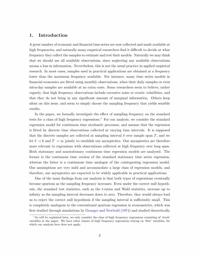
2. Background and Motivation

It is widely observed that test results are critically dependent upon the choice of sampling

frequency in many time series regressions. To illustrate more explicitly the dependency on

the sampling interval of test results, we consider a simple bivariate regression of (yi) on (xi)

written as yi = β0 + β1xi + ui, where β0 and β1 are respectively the intercept and slope

parameters and (ui) are the regression errors. For (yi) and (xi), we consider the following

four pairs:

Model (yi) (xi)

I 10-year T-bond rates 3-month T-bill rates

II 3-month Eurodollar rates 3-month T-bill rates

III log US/UK exchange rates forward log US/UK exchange rates spot

IV log S&P 500 index futures log S&P 500 index

We consider Models I/II primarily as stationary regressions, and Models III/IV as coin-

tegrating regressions. However, whether or not Models I/II and Models III/IV are truly

specified respectively as stationary and cointegrating regressions is not important. Our

asymptotics accommodate both types of regressions.

4

Fig. 1. Data Plots for Models I–IV

1970 1980 1990 2000 20100

5

10

15

20

3-month T-bill10-year T-bond

1975 1980 1985 1990 1995 2000 2005 2010 2015-5

0

5

10

15

20

25

3-month T-bill3-month Eurodollar rates

1980 1985 1990 1995 2000 2005 2010 20150

0.1

0.2

0.3

0.4

0.5

0.6

0.7

0.8

0.9

Spot US/UKForward US/UK

2000 2005 2010 20156.5

7

7.5

8

S&P500S&P500 future

Notes: Presented are daily sample paths of the regressand y and the regressor x used for the empiricalillustrations of Models I–IV. Top-left panel presents the 10-year T-bond rate and 3-month T-bill rate fromJanuary 3, 1962 to March 29, 2018. Top-right panel presents the 3-month Eurodollar rate and 3-monthT-bill rate from January 1, 1971 to October 7, 2016. Bottom-left panel presents the log US/UK 3-monthforward exchange rate and log US/UK spot exchange rate from January 2, 1979 to December 29, 2017.Bottom-right panel presents the log S&P 500 Index future and log S&P 500 Index from September 10, 1997to March 29, 2018.

The plots for (yi) and (xi) in Models I-IV are given in Figure 1.3 In all models, possibly

except for Model I, two series (yi) and (xi) move very closely with each other. Therefore, the

most natural hypothesis to be tested appears to be H0 : β0 = 0 and β1 = 1. The hypothesis

may or may not hold. In particular, the null hypothesis β0 = 0 does not necessarily hold

when there are differences in the term or liquidity premium as well as the general risk

premium between two assets represented by (yi) and (xi). However, in the paper, we do

not intend to provide any answers to whether or not the hypothesis should hold in any of

3The S&P index futures used here and elsewhere in the paper are the log prices of the E-mini S&P 500contracts expiring in the front month (the nearest delivery month) downloaded from Investing.com. TheE-mini S&P 500 contract represents one-fifth of the value of the standard-size futures contract, and it istraded electronically on the Chicago Mercantile Exchange (CME). The E-mini contract has been tradedmuch more actively and widely than the standard contract, and it has become the primary futures tradingvehicle for the S&P 500 index since the inception its trading on September 9, 1997.

5

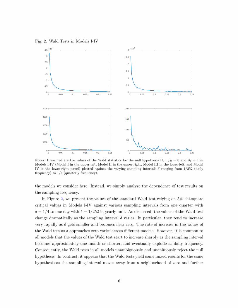
Fig. 2. Wald Tests in Models I-IV

0 0.05 0.1 0.15 0.2 0.250

0.5

1

1.5

2

2.5

3

3.5×104

0 0.05 0.1 0.15 0.2 0.250

0.5

1

1.5

2

2.5

3×104

0 0.05 0.1 0.15 0.2 0.250

1000

2000

3000

4000

5000

0 0.05 0.1 0.15 0.2 0.250

50

100

150

200

Notes: Presented are the values of the Wald statistics for the null hypothesis H0 : β0 = 0 and β1 = 1 inModels I-IV (Model I in the upper-left, Model II in the upper-right, Model III in the lower-left, and ModelIV in the lower-right panel) plotted against the varying sampling intervals δ ranging from 1/252 (dailyfrequency) to 1/4 (quarterly frequency).

the models we consider here. Instead, we simply analyze the dependence of test results on

the sampling frequency.

In Figure 2, we present the values of the standard Wald test relying on 5% chi-square

critical values in Models I-IV against various sampling intervals from one quarter with

δ = 1/4 to one day with δ = 1/252 in yearly unit. As discussed, the values of the Wald test

change dramatically as the sampling interval δ varies. In particular, they tend to increase

very rapidly as δ gets smaller and becomes near zero. The rate of increase in the values of

the Wald test as δ approaches zero varies across different models. However, it is common to

all models that the values of the Wald test start to increase sharply as the sampling interval

becomes approximately one month or shorter, and eventually explode at daily frequency.

Consequently, the Wald tests in all models unambiguously and unanimously reject the null

hypothesis. In contrast, it appears that the Wald tests yield some mixed results for the same

hypothesis as the sampling interval moves away from a neighborhood of zero and further

6

increases.4

The dependency of the test results on the sampling frequency is of course extremely un-

desirable, since in most cases the hypothesis of interest is not specific to sampling frequency

and we expect it to hold for all samples collected at any sampling interval. Subsequently,

we consider a continuous time regression model and build up an appropriate framework to

analyze this dependency of the test results on the sampling frequency. We find that what

we observe here as the common feature of the Wald tests is not an anomaly. From our

asymptotic analysis relying on δ → 0 as well as T → ∞, it actually becomes clear that

the test is expected to diverge up to infinity with probability one as δ decreases down to

zero. Roughly, this happens since the serial correlation at any finite lag of discrete sam-

ples converges to unity as the sampling frequency increases if the samples are taken from

continuous time stochastic processes. We may allow for the presence of jumps, if the jump

activity is regular and there are only a finite number of jumps in any time interval.

3. The Model, Setup and Preliminaries

Consider the standard regression model

yi = x′iβ + ui (1)

for i = 1, . . . , n, where (yi) and (xi) are respectively the regressand and regressor, β is the

regression coefficient and (ui) are the regression errors. Though it is possible to analyze

more general regressions, the simple model we consider here is sufficient to illustrate the

main issue dealt with in the paper. Throughout, we denote by β the OLS estimator of β.

The general linear hypothesis on β, formulated typically as Rβ = r with known matrix R

and vector r of conformable dimensions, is often tested using the Wald statistic defined by

F (β) = (Rβ − r)′R( n∑

i=1

xix′i

)−1R′

−1 (Rβ − r)/σ2, (2)

where σ2 is the usual estimator for the error variance obtained from the OLS residuals (ui).

In the presence of serial correlation in (ui), the Wald statistic introduced in (2) is in general

4We expect that the Wald tests relying on chi-square critical values are subject to nonnegligible sizedistortions, due mainly to the presence of persistency in the regressors and regression errors of our models.Nevertheless, we will not pay attention to this and other related problems of the Wald tests because, asdiscussed, the focus of this paper is to analyze their frequency dependence, not their performance at anyparticular frequency.

7

not applicable. Therefore, in this case, modified versions of the Wald statistic such as

G(β) = (Rβ − r)′R( n∑

i=1

xix′i

)−1R′

−1 (Rβ − r)/ω2, (3)

where ω2 is a consistent estimator for the longrun variance of (ui) based on (ui), or

H(β) = (Rβ − r)′R( n∑

i=1

xix′i

)−1nΩ

(n∑i=1

xix′i

)−1R′

−1 (Rβ − r), (4)

where Ω is a consistent estimator for the longrun variance of (xiui) based on (xiui). We

consider two different types of regressions given by (1): stationary type regression and

cointegration type regression. The test based on (4) is generally more appropriate for the

stationary type regression, whereas only the test based on (3) is sensible for the cointegration

type regression.5

We analyze regression (1), when (yi) and (xi) are high frequency observations.6 For the

subsequent analysis, we let (yi) and (xi) be samples collected at discrete time intervals from

the underlying continuous time processes denoted respectively by Y = (Yt) and X = (Xt),

i.e., we let

yi = Yiδ and xi = Xiδ

for i = 1, . . . , n be discrete samples from the continuous time processes Y and X over time

[0, T ] collected at the sampling interval with length δ > 0, where T = nδ. Our asymptotics

will be obtained by letting δ → 0 and T →∞ jointly. Under our setup, the regression model

introduced in (1) can be analyzed using the corresponding continuous time regression

Yt = X ′tβ + Ut (5)

for 0 ≤ t ≤ T , where Y and X are the regressand and regressor processes, and U = (Ut) is

the error process, from which (ui) are defined similarly as (yi) and (xi) are defined from Y

and X respectively.

The underlying continuous time model in (5), which we rewrite as Yt = α+βXt +Ut in

its simplest form for our discussions below, is introduced to study the type of high frequency

regressions we consider in Section 2. There are other continuous time models that are more

5Note that the longrun variance of (xiui) does not exist if (xi) is nonstationary.6In the paper, high frequency observations are defined to be samples collected at sampling intervals which

are small relative to their time span. For instance, five years of daily observations are considered to be highfrequency observations.

8

suitable to analyze different types of regressions relying on high frequency observations.

Most notably, we may consider a continuous time regression given by

dYt = (α+ βXt)dt+ dUt, (6)

where dU = (dUt) is a martingale differential error, which is often specified further as dUt =

σtdWt for t ≥ 0 with instantaneous volatility σ = (σt) and Brownian motion W = (Wt).

This type of regression is used in Choi et al. (2016) to investigate stock return predictability.

Moreover, we may also look at a continuous time regression of the form

dYt = αdt+ βdXt + dUt, (7)

where dU is defined as in (6). See, e.g., Chang et al. (2016), which uses regression in (7) to

evaluate factor pricing models.

In continuous time regressions, the differentials dY and dX should be used to represent

flow variables like stock or portfolio returns over an infinitesimal interval, whereas the

levels Y and X are more appropriate to specify stock variables such as stock prices, interest

rates and predictive ratios. Also note that we need the dt term to include a constant term

or to relate any stock variable X to a flow variable dY . In the paper, we only consider

the continuous time regression in levels, which is useful to analyze the high frequency

regression modeling a relationship between a ‘stock’ variable and other ‘stock’ covariates.

Therefore, we focus on the continuous time regression (5), and will not consider other types

of continuous time regressions such as (6) and (7). The asymptotics of these continuous

time regressions are quite distinct from our asymptotics in the paper.

For any stochastic process Z = (Zt) appearing in the paper, we assume that Z = Zc+Zd,

where Zc is the continuous part and Zd the jump part defined as Zdt =∑

0≤s≤t ∆Zs with

∆Zt = Zt − Zt−.

Assumption A. Let Z be any element in U2, XX ′ or XU . We have∑0≤t≤T

E|∆Zt| = O(T ).

Moreover, if we define ∆δ,T (Z) = sup0≤s,t≤T sup|t−s|≤δ |Zct − Zcs |, then

max

(δ,δ

Tsup

0≤t≤T|Zt|

)= Op

(∆δ,T (Z)

)

9

as δ → 0 and T →∞.

The conditions in Assumption A are very mild and they are satisfied by virtually all stochas-

tic processes used in both theoretical and empirical applications. The first condition is met,

for instance, for all processes with compound Poisson type jumps as long as their sizes are

bounded in L1 and their intensity is proportional to T . The second condition holds trivially

for a wide class of stochastic processes. If T is fixed, ∆δ,T (Z) represents the usual modulus

of continuity of the stochastic process Z. On the other hand, we let T → ∞ in our setup

and therefore it may be regarded as the global modulus of continuity. Typically, we have

∆δ,T (Z) = δ1/2−ελT (8)

for some ε ≥ 0 and a nonrandom sequence (λT ) of T that is bounded away from zero and,

as an example, the condition is clearly satisfied if sup0≤t≤T |Zt| = Op(T ),7 regardless of how

we set δ and T as long as δ → 0 and T → ∞. The condition holds in any case as long as

δ → 0 fast enough relative to T →∞.8

The following lemma allows us to approximate the sample moments in discrete time by

the corresponding sample moments in continuous time. Here and elsewhere in the paper,

we use ‖ · ‖ to denote the Euclidian norm for a vector or a matrix.

Lemma 3.1. Let Assumption A hold. If we define Z = U2, XX ′ or XU and zi = Ziδ for

i = 1, . . . , n, we have

1

n

n∑i=1

zi =1

T

∫ T

0Ztdt+Op

(∆δ,T (‖Z‖)

)for all small δ and large T .

In our subsequent analysis, we impose a set of sufficient conditions to ensure the asymptotic

negligibility of the approximation error ∆δ,T (‖Z‖), for Z = U2, XX ′ and XU , so that we

may approximate all relevant sample moments by their continuous analog without affecting

their asymptotics. Once the approximations are made, the rest of our asymptotics rely

entirely on the asymptotics of moments in continuous time. This will be introduced below.

7Note that we have sup0≤t≤T |Zt| = Op(√T ) if Z is Brownian motion. Therefore, the condition here is

very mild and expected to be satisfied even by some explosive processes.8This is a necessary condition to guarantee that discretization errors become negligible asymptotically

and our asymptotics are determined solely by those of the underlying continuous time processes. If, forinstance, we set δ → 0 slowly relative to T → ∞, our asymptotics in the paper will not be applicable.Sufficient conditions for the applicability of our asymptotics are dependent on the underlying model andstatistical procedure we use, and they will be introduced later.

10

Assumption B. T−1∫ T

0U2t dt→p σ

2 for some σ2 > 0 as T →∞.

Needless to say, Assumption B holds for a wide variety of asymptotically stationary stochas-

tic processes.

As discussed, we consider two different types of regressions. Below we introduce as-

sumptions for each of these regressions. We denote by D[0, 1] the space of cadlag functions

endowed with the usual Skorohod topology.

Assumption C1. We assume that

(a) T−1∫ T0 XtX

′tdt→p M as T →∞ for some nonrandom matrix M > 0, and

(b) we have

T−1/2∫ T

0XtUtdt→d N(0,Π)

as T →∞, where Π = limT→∞ T−1E

(∫ T0 XtUtdt

)(∫ T0 XtUtdt

)′> 0, which is assumed to

exist.

Assumption C2. We assume that

(a) for XT defined as

XTt = Λ−1T XTt

on [0, 1] with an appropriate nonsingular normalizing sequence (ΛT ) of matrices, we have

XT →d X in the product space of D[0, 1] as T → ∞ with linearly independent limit

process X, and

(b) if we define UT on [0, 1] as

UTt = T−1/2∫ Tt

0Usds,

then UT →d U in D[0, 1] jointly with XT →d X

in the product space of D[0, 1] as T →∞,

where U is Brownian motion with variance π2 = limT→∞ T−1E

(∫ T0 Utdt

)2> 0, which is

assumed to exist.

Both Assumptions C1 and C2 are expected to hold for a wide class of stationary and nonsta-

tionary regressions. Assumption C1 is the continuous analog of the standard assumptions

for stationary regressions in discrete time. Assumption C2(a) is satisfied for general null

recurrent diffusions and jump diffusions, as shown by Jeong and Park (2011), Jeong and

Park (2014) and Kim and Park (2017). Moreover, Assumption C2(b) is the continuous time

version of the usual invariance principle. Note that we assume in Assumption C1 that X

11

and U are uncorrelated as in the standard regression model. However, in Assumption C2,

we allow X and U to be dependent with each other in an arbitrary manner.

In parallel with Assumptions C1 and C2, respectively for the stationary and cointegrat-

ing regressions, we introduce Assumptions D1 and D2 below.

Assumption D1. ∆δ,T (U2),∆δ,T (‖XX ′‖)→p 0 and√T∆δ,T (‖XU‖)→p 0 as δ → 0 and

T →∞.

Assumption D2. ∆δ,T (U2), ‖ΛT ‖2∆δ,T (‖XX ′‖) →p 0 and√T‖ΛT ‖∆δ,T (‖XU‖) →p 0

as δ → 0 and T →∞.

The conditions in Assumptions D1 and D2 hold if δ → 0 fast enough relative to T → ∞.

If the sample paths of U and X are bounded and differentiable with bounded derivatives,

then ∆δ,T (‖Z‖) = Op(δ) for Z = U2, XX ′ and XU and ‖ΛT ‖ = Op(1). In this case, it

suffices to have δ = o(T−1/2). Generally, we require δ → 0 faster relative to T → ∞ if

the underlying processes U and X are more volatile locally and more explosive globally.

If they behave all like Brownian motion, for instance, then we may easily deduce that

∆δ,T (‖Z‖) = Op(δ1/2−εT 1/2+ε

)with an arbitrarily small ε > 0 for Z = U2, XX ′ and XU

from, e.g., Kanaya et al. (2018). Therefore, the conditions in Assumption D1 are met if we

set δ = O(T−2−ε

)for any ε > 0 arbitrarily small. To satisfy the conditions in Assumption

D2, we should have δ → 0 faster, but so much unlessX is overly explosive. If ‖ΛT ‖ = O(√T )

as in the case of X being given by Brownian motion, we only need to require δ = O(T−3−ε

)for ε > 0 arbitrarily small. In sum, our conditions here are not very stringent.

In our asymptotic analysis, we let δ → 0 and T → ∞ jointly, under either Assumption

D1 or D2. Our asymptotics are joint, not sequential, in δ and T . We allow δ → 0 and

T →∞ jointly, as long as δ and T satisfy an appropriate condition specified in Assumption

D1 or D2. In both of these assumptions, we require δ → 0 sufficiently fast relative to

T → ∞. It is therefore expected that our joint asymptotics yield the same results as the

sequential asymptotics relying on δ → 0 followed by T →∞.

4. Spuriousness of Regression at High Frequency

In this section, we establish the asymptotics of the OLS estimator β of β in regression (1)

and analyze the asymptotic behaviors of the standard Wald test based on the test statistic

F (β) in (2) under the null hypothesis H0 : Rβ = r.

12

Theorem 4.1. Assume Rβ = r and let Assumptions A and B hold.

(a) Under Assumption C1, we have

√T (β − β)→d N

δF (β)→d N′R′(RM−1R′

)−1RN/σ2,

where N =d N(0,M−1ΠM−1

), as δ → 0 and T →∞ satisfying Assumption D1.

(b) Under Assumptions C2, we have

√TΛ′T (β − β)→d P

δF (β)→d P′R′(RQ−1R′

)−1RP/σ2

where P =(∫ 1

0 XtX′t dt

)−1 ∫ 10 X

t dU

t and Q =

∫ 10 X

tX′t dt, as δ → 0 and T →∞ satisfy-

ing Assumption D2.

For both stationary and cointegration type regressions, the OLS estimator β is generally

consistent for β under our asymptotics relying on δ → 0 sufficiently fast relative to T →∞.

It is crucial that we have T → ∞ for the consistency of β. If, for instance, T is fixed,

δ → 0 alone is not sufficient for its consistency. On the other hand, for both stationary and

cointegration type regressions, we have

F (β)→p ∞

as δ → 0 and T → ∞. This implies that the Wald test always leads us to reject the null

hypothesis when it is correct, and the asymptotic size becomes unity, as δ → 0 and T →∞.

The regressions therefore become spurious in this sense.

It is easy to see why this happens. Suppose that the law of large numbers and the

central limit theorem hold for U , as we assume in Assumption C1 or C2. Moreover, we

let Assumption A hold for U , and set ∆δ,T (U) →p 0 or more strongly√T∆δ,T (U) →p 0 if

needed as δ → 0 and T →∞. We may easily deduce that

1

n

n∑i=1

ui =1

T

∫ T

0Utdt+ op(1)→p 0

as n→∞ (with δ → 0 and T →∞), and therefore, the law of large numbers holds for (ui).

13

However, we have

1√n

n∑i=1

ui =1√δ

[1√T

∫ T

0Utdt+ op(1)

]→p ∞

as n → ∞ (with δ → 0 and T → ∞), and consequently, the central limit theory fails to

hold for (ui). In fact, in our setup, (ui) becomes strongly dependent as δ → 0, since the

correlation between ui and ui−j for any i and j becomes unity as δ → 0. Therefore, it is

well expected that the central limit theory does not hold for (ui).

Our results here are very much analogous to those from the conventional spurious re-

gression, which was first investigated through simulations by Granger and Newbold (1974)

and explored later analytically by Phillips (1986). As is now well known, the regression of

two independent random walks, or more generally, integrated time series with no cointe-

gration, yields spurious results, and the Wald statistic for testing no longrun relationship

diverges to infinity, implying falsely the presence of cointegration. Granger and Newbold

(1974) originally suggest that this is due to the existence of strong serial dependence in the

regression error. On the other hand, we show in the paper that an authentic relationship in

stationary time series or the presence of cointegration among nonstationary time series is

always rejected if the test is based on the Wald statistic relying on observations collected at

high frequencies. Our spurious regression here is therefore in contrast with the conventional

spurious regression. True relationship is rejected and tested to be false in the former, while

false relationship is rejected and tested to be true in the latter. However, our regression

and the conventional spurious regression have the same reason why they yield nonsensical

results: They both have regression errors that are strongly dependent, and the central limit

theory does not hold for them.

To further analyze the serial dependency in (ui), we consider the AR(1) regression

ui = ρui−1 + εi, (9)

and introduce some additional assumptions in

Assumption E. (a) We let U c, the continuous part of U , be a semimartingale given

by U c = A + M , where A and M are respectively the bounded variation and martingale

components of U c satisfying

sup0≤s,t≤T

|At −As||t− s|

= Op(pT ) and sup0≤s,t≤T

∣∣[M ]t − [M ]s∣∣

|t− s|= Op(qT ),

14

and pT∆δ,T (U)→ 0 and (qT /√T )∆δ,T (U)→ 0 with δ = ∆2

δ,T (U) as δ → 0 and T →∞. (b)

Moreover, we assume that∑

0≤t≤T E(∆Ut)4 = O(T ) and T−1[U ]T →p τ

2 for some τ2 > 0

as T →∞.

The conditions introduced in Assumption E are mild and expected to hold for a wide

class of asymptotically stationary error processes. In Part (a), we require that both the

bounded variation component and the quadratic variation of the martingale component of

the continuous part of the error process U be Lipschitz continuous and δ be small enough

to allow their Lipschitz constants to increase with T . On the other hand, Part (b) holds,

for instance, if the number of jump increases at T -rate and jump size has finite fourth

moment, and if the instantaneous variance of U is asymptotically stationary. Note that

[U ]T = [U c]T +∑

0≤t≤T (∆Ut)2 and [U c]T = [M ]T .

The asymptotics for the estimated AR coefficient ρ of ρ in (9) are given as

Lemma 4.2. Under Assumption E, we have

ρ = 1− τ2

2σ2δ + op(δ)

as δ → 0 and T →∞.

It follows immediately from Lemma 4.2 that

ρ→p 1

particularly as δ → 0. Therefore, (ui) becomes strongly dependent, and the regression

becomes spurious as the sampling interval δ approaches 0. Our regression is completely

analogous to the conventional spurious regression, except that we let δ → 0 in contrast with

the conventional spurious regression requiring n → ∞. Therefore, the results in Theorem

4.1 may well be expected. Though we let T →∞, as well as δ → 0, to get a more explicit

limit of ρ as in Lemma 4.2, the condition T → ∞ is not essential for the spuriousness in

regression (1). This is clear from our proof of Lemma 4.2. If T is assumed to be fixed and

set at T = 1 without loss of generality, we have δ = 1/n and (ui) asymptotically reduces to

a near unit root process with AR coefficient ρ = 1− c/n with c = τ2/2σ2.

Of course, it is also possible to formulate and analyze the classical spurious regression

in continuous time. If the underlying regression error process U is indeed nonstationary

and has a stochastic trend, we have T−1∫ T0 U2

t dt →p ∞ as T → ∞. Therefore, we expect

that our regression becomes spurious as long as T is large even if δ is not small. In the

paper, however, we assume T−1∫ T0 U2

t dt →p σ2 as T → ∞, and let δ → 0 to analyze the

15

spuriousness generated by high frequency observations. In our setup, the regression error

(ui) becomes strongly persistent and the regression becomes spurious, simply because we

collect samples too frequently.

The speed at which ρ diverges away from the unity as δ increases depends on the ratio

τ2/σ2. Roughly, τ2 measures the mean local variation, while σ2 represents the mean global

variation of the error process U . Therefore, we may refer to it as the local-to-global variation

ratio. The larger the value of the ratio is, the slower ρ converges to the unity as δ → 0.

Note that the ratio becomes large if, in particular, either the existence of excessive volatility

makes local variation large, or the presence of strong mean reversion makes global variation

small. If U is the Ornstein-Uhlenbeck process given by dUt = −κUtdt + υdWt, we have

τ2 = υ2 and σ2 = υ2/2κ. Therefore, the ratio becomes τ2/σ2 = 2κ, which becomes larger if

we have stronger mean reversion. The local-to-global variation ratios of U estimated using

the fitted residuals of Models I-IV are 1.08, 14.30, 3.16 and 169.9, respectively. The ratio

is particularly large for Model IV, which explains why its estimated residual AR coefficient

is not quite close to the unity at the highest frequency, daily.

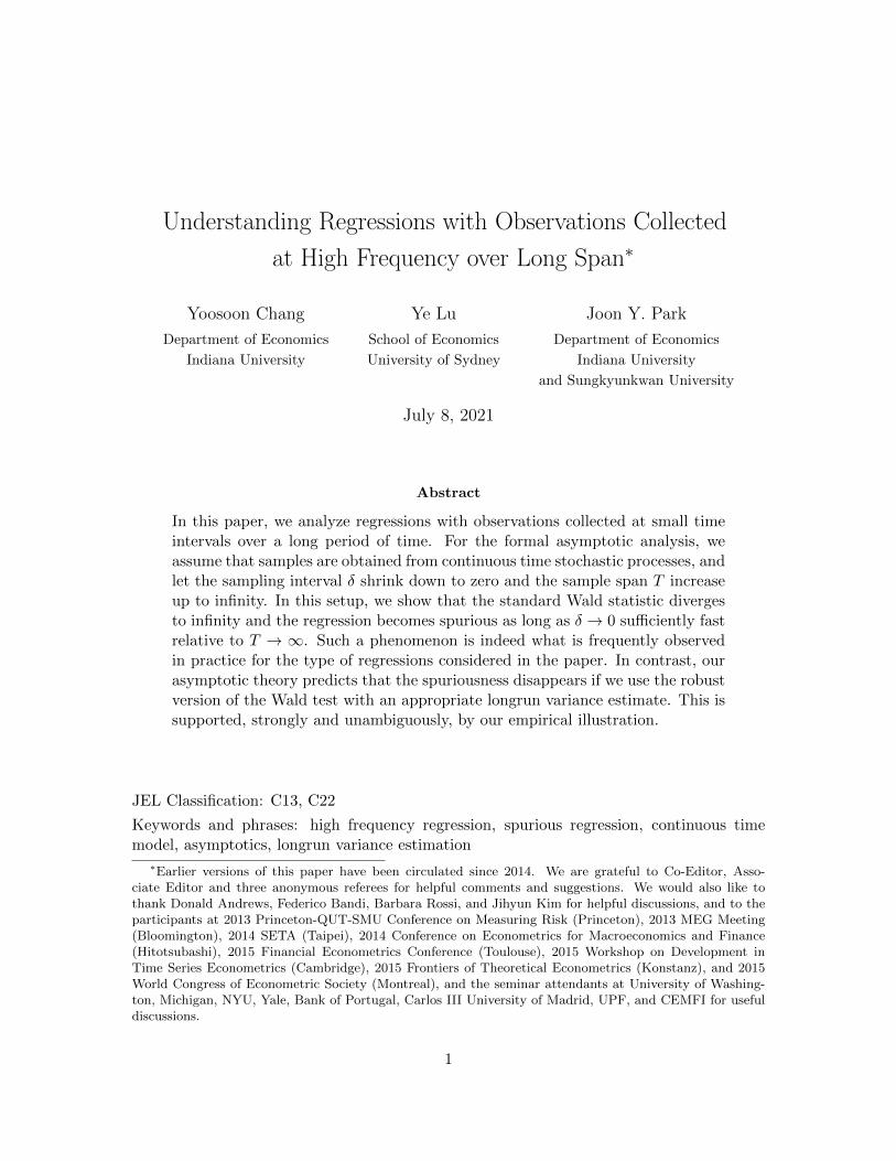
The actual estimates of the autoregressive coefficients for the fitted residuals from Models

I-IV are plotted in Figure 3 against various values of the sampling interval. It is clearly

seen that the estimates of the autoregressive coefficients tend to increase as the sampling

interval shrinks. In particular, except for Model IV, the estimates approach unity as the

sampling interval decreases. This is exactly what we expect from Lemma 4.2. Model IV

is rather exceptional. For Model IV, the estimated autoregressive coefficients do not show

any monotonous increasing trend, unlike all other models. In fact, Lemma 4.2 does not

seem to apply for Model IV, which alludes that Assumption E does not hold for Model

IV. This is perhaps due to more irregular and frequent jump activities present in stock

prices than are allowed in Assumption E. Of course, not all types of jumps are permitted

in our paper, though our assumptions on jumps are fairly general and weak. In particular,

we assume that the jump intensity is proportional to time span, following most of the

existing literature, which excludes the possibility of having jumps with intensity varying

with sampling frequency.

Needless to say, all our analysis for (ui) applies also to any linear combination of the

vector time series (xiui), (c′xiui) for an arbitrary nonrandom vector c, say, if we assume

the vector process c′XU satisfies the same conditions as those we impose on U above in

Assumption E.

16

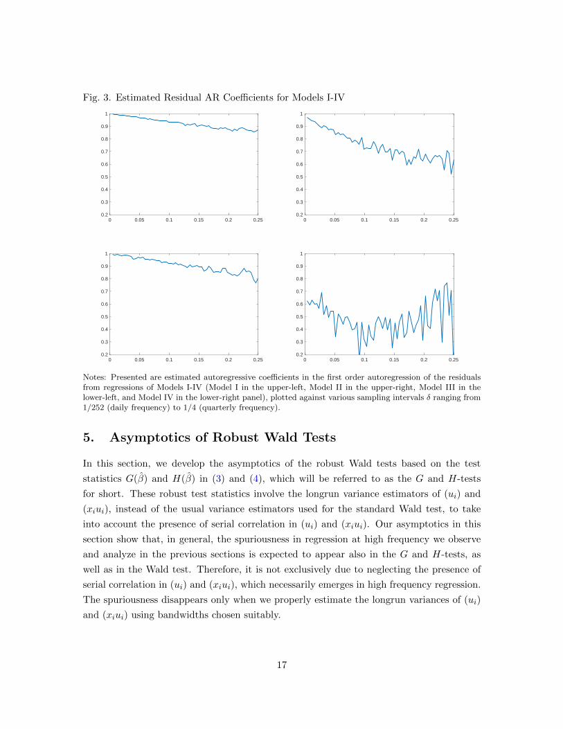
Fig. 3. Estimated Residual AR Coefficients for Models I-IV

0 0.05 0.1 0.15 0.2 0.250.2

0.3

0.4

0.5

0.6

0.7

0.8

0.9

1

0 0.05 0.1 0.15 0.2 0.250.2

0.3

0.4

0.5

0.6

0.7

0.8

0.9

1

0 0.05 0.1 0.15 0.2 0.250.2

0.3

0.4

0.5

0.6

0.7

0.8

0.9

1

0 0.05 0.1 0.15 0.2 0.250.2

0.3

0.4

0.5

0.6

0.7

0.8

0.9

1

Notes: Presented are estimated autoregressive coefficients in the first order autoregression of the residualsfrom regressions of Models I-IV (Model I in the upper-left, Model II in the upper-right, Model III in thelower-left, and Model IV in the lower-right panel), plotted against various sampling intervals δ ranging from1/252 (daily frequency) to 1/4 (quarterly frequency).

5. Asymptotics of Robust Wald Tests

In this section, we develop the asymptotics of the robust Wald tests based on the test

statistics G(β) and H(β) in (3) and (4), which will be referred to as the G and H-tests

for short. These robust test statistics involve the longrun variance estimators of (ui) and

(xiui), instead of the usual variance estimators used for the standard Wald test, to take

into account the presence of serial correlation in (ui) and (xiui). Our asymptotics in this

section show that, in general, the spuriousness in regression at high frequency we observe

and analyze in the previous sections is expected to appear also in the G and H-tests, as

well as in the Wald test. Therefore, it is not exclusively due to neglecting the presence of

serial correlation in (ui) and (xiui), which necessarily emerges in high frequency regression.

The spuriousness disappears only when we properly estimate the longrun variances of (ui)

and (xiui) using bandwidths chosen suitably.

17

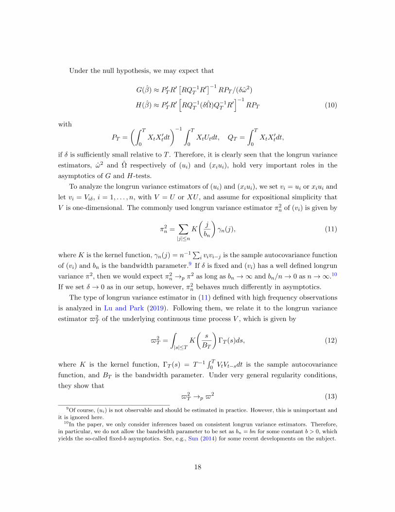
Under the null hypothesis, we may expect that

G(β) ≈ P ′TR′[RQ−1T R′

]−1RPT /(δω

2)

H(β) ≈ P ′TR′[RQ−1T (δΩ)Q−1T R′

]−1RPT (10)

with

PT =

(∫ T

0XtX

′tdt

)−1 ∫ T

0XtUtdt, QT =

∫ T

0XtX

′tdt,

if δ is sufficiently small relative to T . Therefore, it is clearly seen that the longrun variance

estimators, ω2 and Ω respectively of (ui) and (xiui), hold very important roles in the

asymptotics of G and H-tests.

To analyze the longrun variance estimators of (ui) and (xiui), we set vi = ui or xiui and

let vi = Viδ, i = 1, . . . , n, with V = U or XU , and assume for expositional simplicity that

V is one-dimensional. The commonly used longrun variance estimator π2n of (vi) is given by

π2n =∑|j|≤n

K

(j

bn

)γn(j), (11)

where K is the kernel function, γn(j) = n−1∑

i vivi−j is the sample autocovariance function

of (vi) and bn is the bandwidth parameter.9 If δ is fixed and (vi) has a well defined longrun

variance π2, then we would expect π2n →p π2 as long as bn →∞ and bn/n→ 0 as n→∞.10

If we set δ → 0 as in our setup, however, π2n behaves much differently in asymptotics.

The type of longrun variance estimator in (11) defined with high frequency observations

is analyzed in Lu and Park (2019). Following them, we relate it to the longrun variance

estimator $2T of the underlying continuous time process V , which is given by

$2T =

∫|s|≤T

K

(s

BT

)ΓT (s)ds, (12)

where K is the kernel function, ΓT (s) = T−1∫ T0 VtVt−sdt is the sample autocovariance

function, and BT is the bandwidth parameter. Under very general regularity conditions,

they show that

$2T →p $

2 (13)

9Of course, (ui) is not observable and should be estimated in practice. However, this is unimportant andit is ignored here.

10In the paper, we only consider inferences based on consistent longrun variance estimators. Therefore,in particular, we do not allow the bandwidth parameter to be set as bn = bn for some constant b > 0, whichyields the so-called fixed-b asymptotics. See, e.g., Sun (2014) for some recent developments on the subject.

18

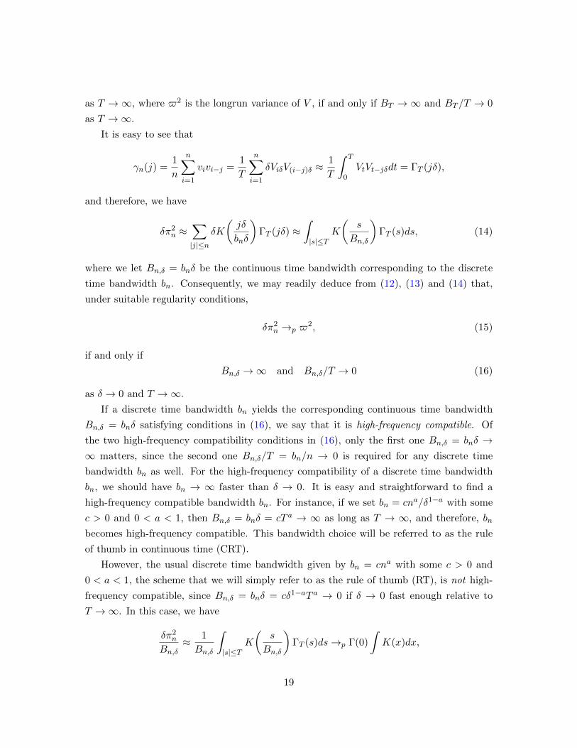
as T →∞, where $2 is the longrun variance of V , if and only if BT →∞ and BT /T → 0

as T →∞.

It is easy to see that

γn(j) =1

n

n∑i=1

vivi−j =1

T

n∑i=1

δViδV(i−j)δ ≈1

T

∫ T

0VtVt−jδdt = ΓT (jδ),

and therefore, we have

δπ2n ≈∑|j|≤n

δK

(jδ

bnδ

)ΓT (jδ) ≈

∫|s|≤T

K

(s

Bn,δ

)ΓT (s)ds, (14)

where we let Bn,δ = bnδ be the continuous time bandwidth corresponding to the discrete

time bandwidth bn. Consequently, we may readily deduce from (12), (13) and (14) that,

under suitable regularity conditions,

δπ2n →p $2, (15)

if and only if

Bn,δ →∞ and Bn,δ/T → 0 (16)

as δ → 0 and T →∞.

If a discrete time bandwidth bn yields the corresponding continuous time bandwidth

Bn,δ = bnδ satisfying conditions in (16), we say that it is high-frequency compatible. Of

the two high-frequency compatibility conditions in (16), only the first one Bn,δ = bnδ →∞ matters, since the second one Bn,δ/T = bn/n → 0 is required for any discrete time

bandwidth bn as well. For the high-frequency compatibility of a discrete time bandwidth

bn, we should have bn → ∞ faster than δ → 0. It is easy and straightforward to find a

high-frequency compatible bandwidth bn. For instance, if we set bn = cna/δ1−a with some

c > 0 and 0 < a < 1, then Bn,δ = bnδ = cT a → ∞ as long as T → ∞, and therefore, bn

becomes high-frequency compatible. This bandwidth choice will be referred to as the rule

of thumb in continuous time (CRT).

However, the usual discrete time bandwidth given by bn = cna with some c > 0 and

0 < a < 1, the scheme that we will simply refer to as the rule of thumb (RT), is not high-

frequency compatible, since Bn,δ = bnδ = cδ1−aT a → 0 if δ → 0 fast enough relative to

T →∞. In this case, we have

δπ2nBn,δ

≈ 1

Bn,δ

∫|s|≤T

K

(s

Bn,δ

)ΓT (s)ds→p Γ(0)

∫K(x)dx,

19

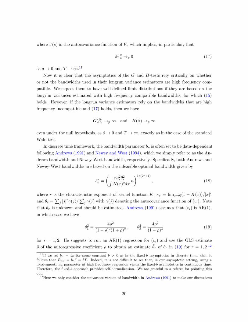
where Γ(s) is the autocovariance function of V , which implies, in particular, that

δπ2n →p 0 (17)

as δ → 0 and T →∞.11

Now it is clear that the asymptotics of the G and H-tests rely critically on whether

or not the bandwidths used in their longrun variance estimators are high frequency com-

patible. We expect them to have well defined limit distributions if they are based on the

longrun variances estimated with high frequency compatible bandwidths, for which (15)

holds. However, if the longrun variance estimators rely on the bandwidths that are high

frequency incompatible and (17) holds, then we have

G(β)→p ∞ and H(β)→p ∞

even under the null hypothesis, as δ → 0 and T →∞, exactly as in the case of the standard

Wald test.

In discrete time framework, the bandwidth parameter bn is often set to be data-dependent

following Andrews (1991) and Newey and West (1994), which we simply refer to as the An-

drews bandwidth and Newey-West bandwidth, respectively. Specifically, both Andrews and

Newey-West bandwidths are based on the infeasible optimal bandwidth given by

b∗n =

(rκ2rθ

2r∫

K(x)2dxn

)1/(2r+1)

, (18)

where r is the characteristic exponent of kernel function K, κr = limx→0(1 − K(x))/|x|r

and θr =∑

j |j|rγ(j)/∑

j γ(j) with γ(j) denoting the autocovariance function of (vi). Note

that θr is unknown and should be estimated. Andrews (1991) assumes that (vi) is AR(1),

in which case we have

θ21 =4ρ2

(1− ρ)2(1 + ρ)2, θ22 =

4ρ2

(1− ρ)4(19)

for r = 1, 2. He suggests to run an AR(1) regression for (vi) and use the OLS estimate

ρ of the autoregressive coefficient ρ to obtain an estimate θr of θr in (19) for r = 1, 2.12

11If we set bn = bn for some constant b > 0 as in the fixed-b asymptotics in discrete time, then itfollows that Bn,δ = bnδ = bT . Indeed, it is not difficult to see that, in our asymptotic setting, using afixed-smoothing parameter at high frequency regression yields the fixed-b asymptotics in continuous time.Therefore, the fixed-b approach provides self-normalization. We are grateful to a referee for pointing thisout.

12Here we only consider the univariate version of bandwidth in Andrews (1991) to make our discussions

20

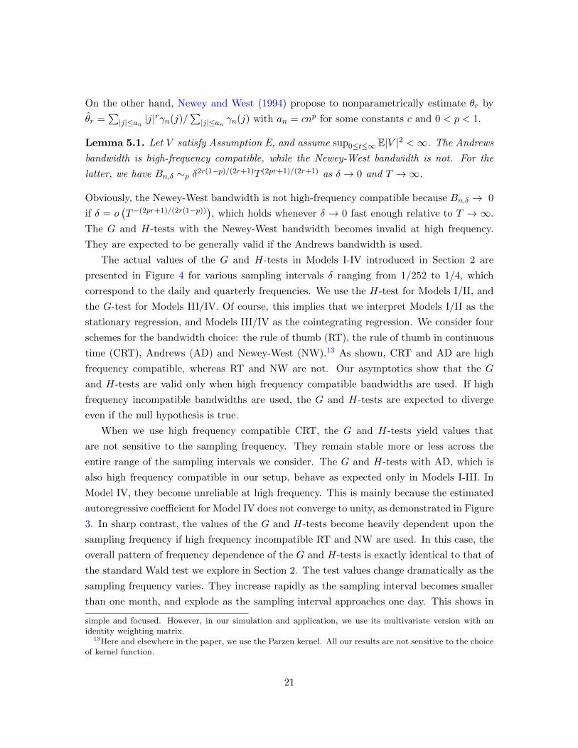
On the other hand, Newey and West (1994) propose to nonparametrically estimate θr by

θr =∑|j|≤an |j|

rγn(j)/∑|j|≤an γn(j) with an = cnp for some constants c and 0 < p < 1.

Lemma 5.1. Let V satisfy Assumption E, and assume sup0≤t≤∞ E|V |2 <∞. The Andrews

bandwidth is high-frequency compatible, while the Newey-West bandwidth is not. For the

latter, we have Bn,δ ∼p δ2r(1−p)/(2r+1)T (2pr+1)/(2r+1) as δ → 0 and T →∞.

Obviously, the Newey-West bandwidth is not high-frequency compatible because Bn,δ → 0

if δ = o(T−(2pr+1)/(2r(1−p))), which holds whenever δ → 0 fast enough relative to T → ∞.

The G and H-tests with the Newey-West bandwidth becomes invalid at high frequency.

They are expected to be generally valid if the Andrews bandwidth is used.

The actual values of the G and H-tests in Models I-IV introduced in Section 2 are

presented in Figure 4 for various sampling intervals δ ranging from 1/252 to 1/4, which

correspond to the daily and quarterly frequencies. We use the H-test for Models I/II, and

the G-test for Models III/IV. Of course, this implies that we interpret Models I/II as the

stationary regression, and Models III/IV as the cointegrating regression. We consider four

schemes for the bandwidth choice: the rule of thumb (RT), the rule of thumb in continuous

time (CRT), Andrews (AD) and Newey-West (NW).13 As shown, CRT and AD are high

frequency compatible, whereas RT and NW are not. Our asymptotics show that the G

and H-tests are valid only when high frequency compatible bandwidths are used. If high

frequency incompatible bandwidths are used, the G and H-tests are expected to diverge

even if the null hypothesis is true.

When we use high frequency compatible CRT, the G and H-tests yield values that

are not sensitive to the sampling frequency. They remain stable more or less across the

entire range of the sampling intervals we consider. The G and H-tests with AD, which is

also high frequency compatible in our setup, behave as expected only in Models I-III. In

Model IV, they become unreliable at high frequency. This is mainly because the estimated

autoregressive coefficient for Model IV does not converge to unity, as demonstrated in Figure

3. In sharp contrast, the values of the G and H-tests become heavily dependent upon the

sampling frequency if high frequency incompatible RT and NW are used. In this case, the

overall pattern of frequency dependence of the G and H-tests is exactly identical to that of

the standard Wald test we explore in Section 2. The test values change dramatically as the

sampling frequency varies. They increase rapidly as the sampling interval becomes smaller

than one month, and explode as the sampling interval approaches one day. This shows in

simple and focused. However, in our simulation and application, we use its multivariate version with anidentity weighting matrix.

13Here and elsewhere in the paper, we use the Parzen kernel. All our results are not sensitive to the choiceof kernel function.

21

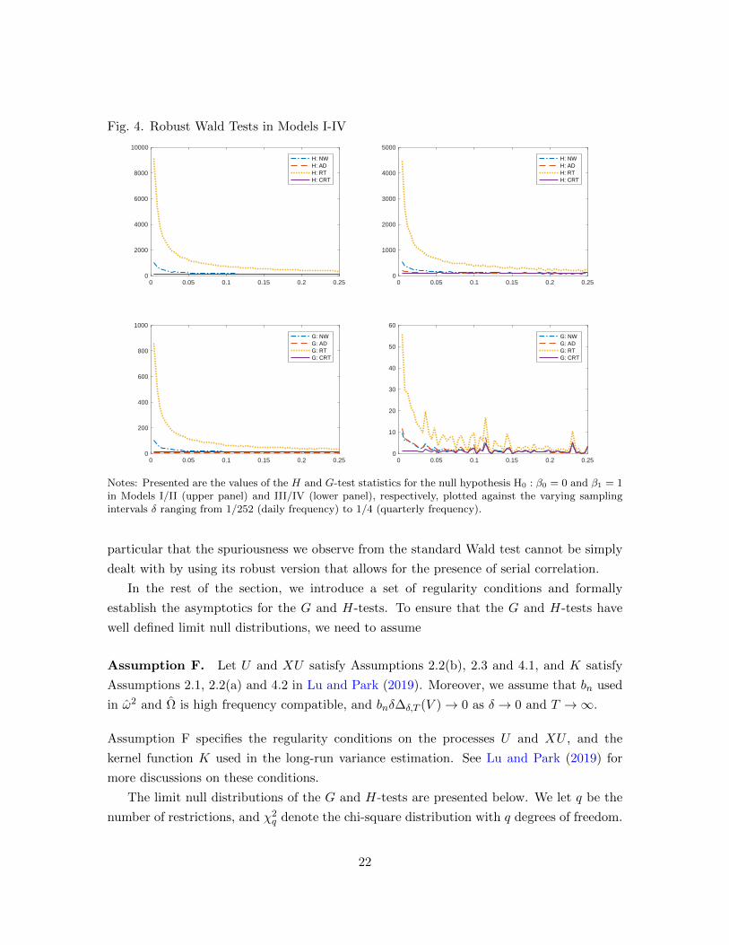
Fig. 4. Robust Wald Tests in Models I-IV

0 0.05 0.1 0.15 0.2 0.250

2000

4000

6000

8000

10000

H: NWH: ADH: RTH: CRT

0 0.05 0.1 0.15 0.2 0.250

1000

2000

3000

4000

5000

H: NWH: ADH: RTH: CRT

0 0.05 0.1 0.15 0.2 0.250

200

400

600

800

1000

G: NWG: ADG: RTG: CRT

0 0.05 0.1 0.15 0.2 0.250

10

20

30

40

50

60

G: NWG: ADG: RTG: CRT

Notes: Presented are the values of the H and G-test statistics for the null hypothesis H0 : β0 = 0 and β1 = 1in Models I/II (upper panel) and III/IV (lower panel), respectively, plotted against the varying samplingintervals δ ranging from 1/252 (daily frequency) to 1/4 (quarterly frequency).

particular that the spuriousness we observe from the standard Wald test cannot be simply

dealt with by using its robust version that allows for the presence of serial correlation.

In the rest of the section, we introduce a set of regularity conditions and formally

establish the asymptotics for the G and H-tests. To ensure that the G and H-tests have

well defined limit null distributions, we need to assume

Assumption F. Let U and XU satisfy Assumptions 2.2(b), 2.3 and 4.1, and K satisfy

Assumptions 2.1, 2.2(a) and 4.2 in Lu and Park (2019). Moreover, we assume that bn used

in ω2 and Ω is high frequency compatible, and bnδ∆δ,T (V )→ 0 as δ → 0 and T →∞.

Assumption F specifies the regularity conditions on the processes U and XU , and the

kernel function K used in the long-run variance estimation. See Lu and Park (2019) for

more discussions on these conditions.

The limit null distributions of the G and H-tests are presented below. We let q be the

number of restrictions, and χ2q denote the chi-square distribution with q degrees of freedom.

22

Theorem 5.2. Assume Rβ = r and let Assumptions A and F hold.

(a) Under Assumptions C1 and D1, we have

H(β)→d χ2q

as δ → 0 and T →∞.

(b) Under Assumptions C2 and D2, we have

G(β)→d P∗′R′

(RQ−1R′

)−1RP ∗

as δ → 0 and T → ∞, where P ∗ =(∫ 1

0 XtX′t dt

)−1 ∫ 10 X

t dU

∗t with standard Brownian

motion U∗ defined as U∗ = U/ω and Q =∫ 10 X

tX′t dt using the notations in Theorem 4.1.

Both G and H-tests have well defined limit null distributions respectively for general sta-

tionary and nonstationary regressions, if in particular we use high-frequency compatible

bandwidths for their longrun variance estimates. The H-test has the standard chi-square

limit null distribution for stationary regressions. On the other hand, the limit null dis-

tribution of the G-test is generally nonnormal and nonstandard. If, however, the limit

processes X and U are independent, then its limit null distribution reduces to chi-square

distribution.

6. An Empirical Illustration

In this section, we investigate the extent to which the interest rates of securities with time

varying maturities move together using the tests introduced in the previous section. To

eliminate default probabilities as a confounding factor, we consider U.S. treasury bonds

and study specifically interest rate co-movement along the U.S. treasury yield curve. Our

question can then be posed alternatively as to whether or not the slope of the yield curve

remains constant in response to an economic shock, for example an unexpected change in

monetary policy. We will say if interest rates along the yield curve move together that the

data supports the idea of a “parallel shift” in the yield curve. A parallel shift occurs when,

for example, a twenty-five basis point increase in the federal funds rate is associated with

a twenty-five basis point increase in the ten-year yield. We are agnostic as to whether a

parallel yield curve shift is associated with the state of the economy. This parallel shift may

therefore happen in normal times, characterized with a typical upward sloping yield curve

and also in bad times, when a flat or inverted yield curve is more common.

The consistent co-movement of long and short rates, should we establish this as a styl-

23

ized fact, would have important monetary policy implications. Such a finding would imply

that the U.S. Federal Reserve System (FED) could effectively control long rates simply by

manipulating the short-term policy rate, the federal funds rate (FFR), through traditional

open market operations. The targeting of rates had indeed been one of the conventional

monetary policy tools employed by the FED over the past four decades to execute its

dual mandate.14 The FED’s efforts to counter the negative shocks associated with the

financial market meltdown in 2008-9 were challenged by the fact that nominal rates had

fallen quite dramatically in the decade preceding the crisis, due in large part to persistently

low inflation expectations (Bernanke (2020)). In an environment with the policy rate at

or near the zero lower bound (ZLB), the FED was compelled to consider implementing

a set of non-conventional policy tools, including most notably quantitative easing (QE),

forward guidance, large scale asset purchases (LSAP), repurchase agreement (REPO), re-

verse REPO, negative interest rates and yield curve control. These non-conventional tools

would allow for the continued provision of an accommodative monetary policy despite the

constraints imposed by the ZLB.

The FED actually implemented many of these non-conventional monetary policy tools

during and after the 2008-9 financial crisis. With these non-conventional monetary policies,

the FED hoped to directly affect long rates in spite of its inability to further lower nomi-

nal short term rates - as the latter had been either at or near the zero lower bound since

the crisis.15 Long rates, of course, may change independently of the FED due to portfolio

reallocation strategies by investors that reflect state specific risk and expected return fore-

casts by asset class over the course of the business cycle. Nevertheless, the unconventional

policies, QE and forward guidance in particular, turned out to be effective for the FED

to achieve its dual mandate of achieving maximum employment and stable inflation not

only during the crisis but also for many years thereafter. Naturally the uncertainties about

the effectiveness of these non-conventional policies have been diminished, and these policy

tools seem no longer considered as non-conventional. Rather, they are now considered to

be effective policy tools that provide policy makers with even more operating flexibility to

support the economy and financial markets in times of great distress (Bernanke (2020)).

Now we test empirically if the FED has indeed controlled long rates by manipulating the

short term policy rate until the 2008-9 financial crisis. Specifically, we consider the simple

14The other monetary policy tool used is the targeting of monetary aggregates such as M2. The FEDChairman Alan Greenspan noted in July 1993 testimony to Congress that this policy tool was no longeruseful.

15Interest rates hit the zero lower bound in September 2008. The three-month secondary market rate was0.03% on September 17, 2008, and the FED made its first purchase of financial assets in November 2008.

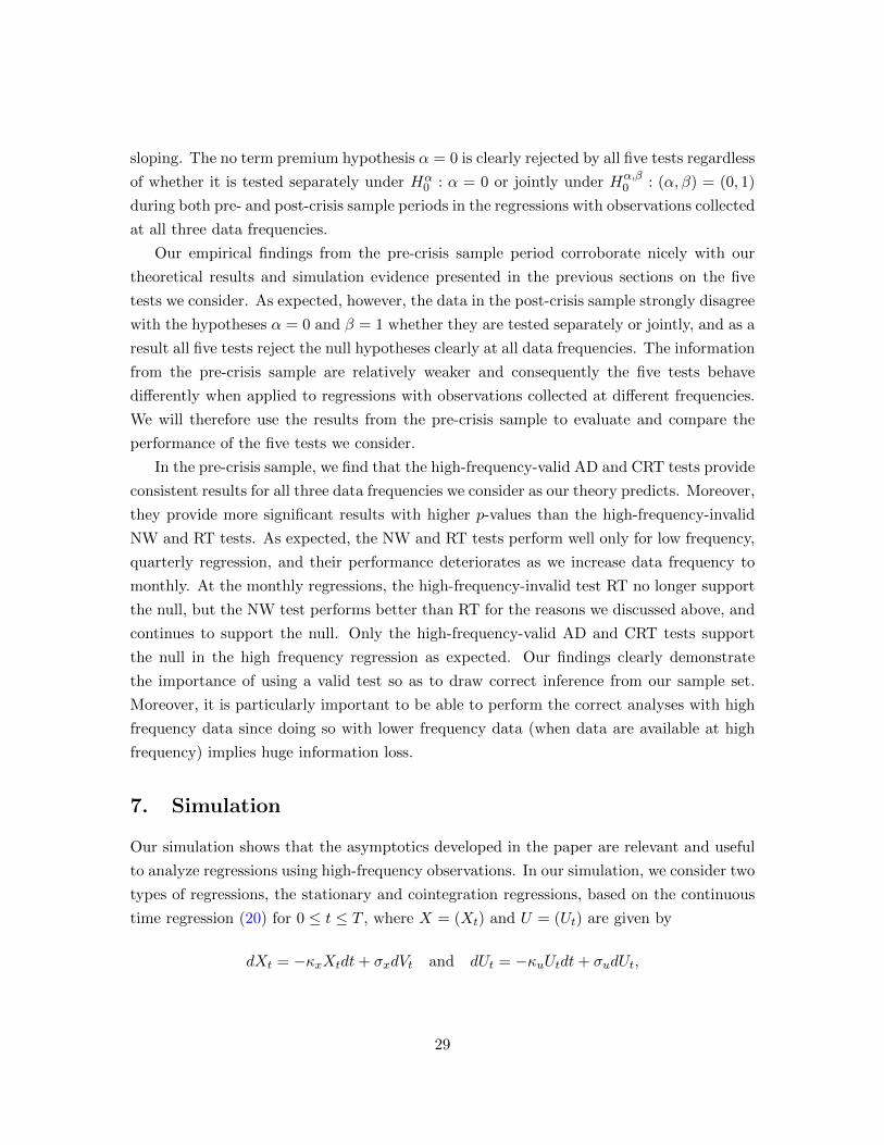
24

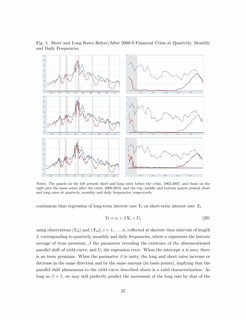
Fig. 5. Short and Long Rates Before/After 2008-9 Financial Crisis at Quarterly, Monthlyand Daily Frequencies

Notes: The panels on the left present short and long rates before the crisis, 1962-2007, and those on theright plot the same series after the crisis, 2008-2019, and the top, middle and bottom panels present shortand long rates at quarterly, monthly and daily frequencies, respectively.

continuous time regression of long-term interest rate Yt on short-term interest rate Xt

Yt = α+ βXt + Ut (20)

using observations (Yiδ) and (Xiδ), i = 1, . . . , n, collected at discrete time intervals of length

δ, corresponding to quarterly, monthly and daily frequencies, where α represents the historic

average of term premium, β the parameter revealing the existence of the aforementioned

parallel shift of yield curve, and Ut the regression error. When the intercept α is zero, there

is no term premium. When the parameter β is unity, the long and short rates increase or

decrease in the same direction and by the same amount (in basis points), implying that the

parallel shift phenomena to the yield curve described above is a valid characterization. As

long as β = 1, we may still perfectly predict the movement of the long rate by that of the

25

short rate conditional on the term premium. Therefore non-rejection of β = 1 may provide

an empirical justification for FED’s efforts to influence long rates through its usual open

market operations.

We use the interest rate on the ten-year U.S. Treasury bond for the long-term interest

rate (Yiδ), and the three-month U.S. Treasury bill secondary market rate for the short-term

rate (Xiδ). Both data series are obtained at quarterly, monthly and daily frequencies from

the Federal Reserve Economic Data (FRED) of St. Louis FED. The two interest rates at

quarterly, monthly and daily frequencies are plotted in Figure 5 where the panels on the

left and right are respectively for the sample periods before and after the 2008-9 financial

crisis, 1962-2007 and 2008-2019. The shaded areas indicate the NBER recessions. We start

from 1962 when the 10 year rate became available at daily frequency.

We test if α = 0 and β = 1 both separately and jointly under the null hypotheses

Hα0 : α = 0, Hβ

0 : β = 1, and Hα,β0 : (α, β) = (0, 1) for the pre- and post-crisis sample periods

using the four robust H-tests, AD, CRT, NW and RT, as well as the non-robust Wald test

introduced in the previous section. All tests are valid asymptotically for low frequency data.

The non-robust Wald test is valid only for the regressions with observations collected at

low frequency. For the regressions with observations collected at high frequency, however,

only two robust H-tests, AD and CRT, are valid according to our theoretical results and

simulation evidence. The other two robust tests, NW and RT, are valid only in low frequency

regressions. For easy reference, we call the AD and CRT as high-frequency-valid tests and

NW and RT as high-frequency-invalid tests.

To empirically demonstrate this point, we test our hypotheses using both low frequency

(quarterly) and high frequency (daily) data. Monthly data are also considered for compari-

son. In fact, they can be considered as either low or high frequency depending on the sample

size. Recall that our asymptotics are applicable only when δ → 0 sufficiently fast relative to

T →∞. High-frequency-invalid tests may behave well at monthly frequency if their diver-

gence rates are not too fast. As we show in our simulations, the high-frequency-invalid NW

test diverges more slowly as the sampling interval decreases than the other high-frequency-

invalid RT test, and thus it may perform better than RT at monthly frequency.

The test results from the quarterly, monthly and daily regressions are presented in

Figure 1, Figure 2 and Figure 3, respectively. The results from the pre- and post-crisis

samples are presented in the upper and lower panels in each table. The test values along

with the 1% and 5% critical values for the five tests considered are presented. For the

robust tests on Hβ0 for pre-crisis samples, the p-values are also provided. The test values

and the associated p-values are marked with one star (two stars) when the null hypothesis is

rejected at 5% (1%) significance level. Non-rejection of a null hypothesis at 5% significance

26

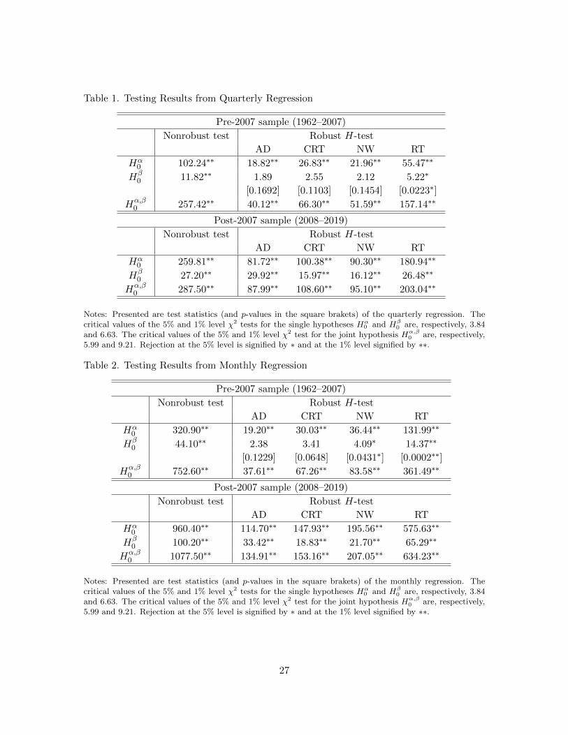
Table 1. Testing Results from Quarterly Regression

Pre-2007 sample (1962–2007)

Nonrobust test Robust H-test

AD CRT NW RT

Hα0 102.24∗∗ 18.82∗∗ 26.83∗∗ 21.96∗∗ 55.47∗∗

Hβ0 11.82∗∗ 1.89 2.55 2.12 5.22∗

[0.1692] [0.1103] [0.1454] [0.0223∗]

Hα,β0 257.42∗∗ 40.12∗∗ 66.30∗∗ 51.59∗∗ 157.14∗∗

Post-2007 sample (2008–2019)

Nonrobust test Robust H-test

AD CRT NW RT

Hα0 259.81∗∗ 81.72∗∗ 100.38∗∗ 90.30∗∗ 180.94∗∗

Hβ0 27.20∗∗ 29.92∗∗ 15.97∗∗ 16.12∗∗ 26.48∗∗

Hα,β0 287.50∗∗ 87.99∗∗ 108.60∗∗ 95.10∗∗ 203.04∗∗

Notes: Presented are test statistics (and p-values in the square brakets) of the quarterly regression. Thecritical values of the 5% and 1% level χ2 tests for the single hypotheses Hα

0 and Hβ0 are, respectively, 3.84

and 6.63. The critical values of the 5% and 1% level χ2 test for the joint hypothesis Hα,β0 are, respectively,

5.99 and 9.21. Rejection at the 5% level is signified by ∗ and at the 1% level signified by ∗∗.

Table 2. Testing Results from Monthly Regression

Pre-2007 sample (1962–2007)

Nonrobust test Robust H-test

AD CRT NW RT

Hα0 320.90∗∗ 19.20∗∗ 30.03∗∗ 36.44∗∗ 131.99∗∗

Hβ0 44.10∗∗ 2.38 3.41 4.09∗ 14.37∗∗

[0.1229] [0.0648] [0.0431∗] [0.0002∗∗]

Hα,β0 752.60∗∗ 37.61∗∗ 67.26∗∗ 83.58∗∗ 361.49∗∗

Post-2007 sample (2008–2019)

Nonrobust test Robust H-test

AD CRT NW RT

Hα0 960.40∗∗ 114.70∗∗ 147.93∗∗ 195.56∗∗ 575.63∗∗

Hβ0 100.20∗∗ 33.42∗∗ 18.83∗∗ 21.70∗∗ 65.29∗∗

Hα,β0 1077.50∗∗ 134.91∗∗ 153.16∗∗ 207.05∗∗ 634.23∗∗

Notes: Presented are test statistics (and p-values in the square brakets) of the monthly regression. Thecritical values of the 5% and 1% level χ2 tests for the single hypotheses Hα

0 and Hβ0 are, respectively, 3.84

and 6.63. The critical values of the 5% and 1% level χ2 test for the joint hypothesis Hα,β0 are, respectively,

5.99 and 9.21. Rejection at the 5% level is signified by ∗ and at the 1% level signified by ∗∗.

27

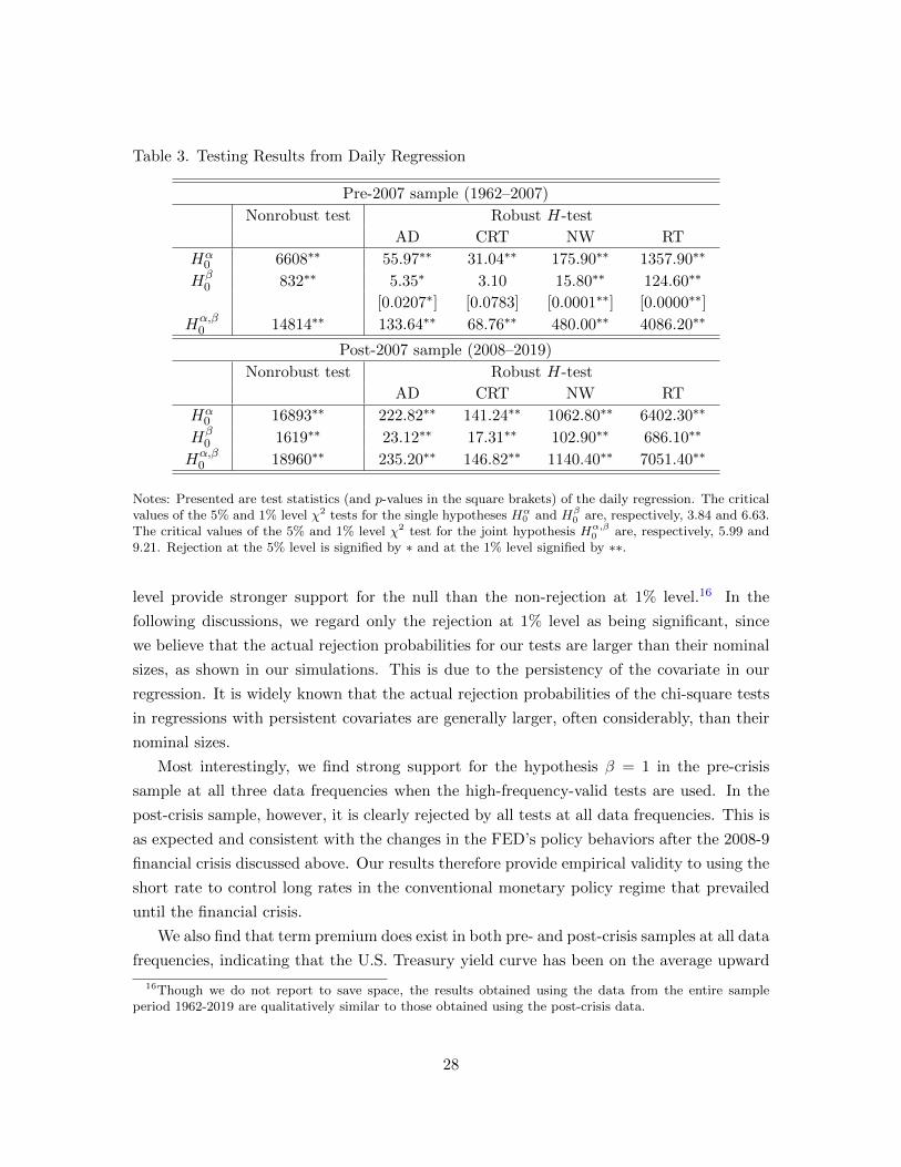
Table 3. Testing Results from Daily Regression

Pre-2007 sample (1962–2007)

Nonrobust test Robust H-test

AD CRT NW RT

Hα0 6608∗∗ 55.97∗∗ 31.04∗∗ 175.90∗∗ 1357.90∗∗

Hβ0 832∗∗ 5.35∗ 3.10 15.80∗∗ 124.60∗∗

[0.0207∗] [0.0783] [0.0001∗∗] [0.0000∗∗]

Hα,β0 14814∗∗ 133.64∗∗ 68.76∗∗ 480.00∗∗ 4086.20∗∗

Post-2007 sample (2008–2019)

Nonrobust test Robust H-test

AD CRT NW RT

Hα0 16893∗∗ 222.82∗∗ 141.24∗∗ 1062.80∗∗ 6402.30∗∗

Hβ0 1619∗∗ 23.12∗∗ 17.31∗∗ 102.90∗∗ 686.10∗∗

Hα,β0 18960∗∗ 235.20∗∗ 146.82∗∗ 1140.40∗∗ 7051.40∗∗

Notes: Presented are test statistics (and p-values in the square brakets) of the daily regression. The criticalvalues of the 5% and 1% level χ2 tests for the single hypotheses Hα

0 and Hβ0 are, respectively, 3.84 and 6.63.

The critical values of the 5% and 1% level χ2 test for the joint hypothesis Hα,β0 are, respectively, 5.99 and

9.21. Rejection at the 5% level is signified by ∗ and at the 1% level signified by ∗∗.

level provide stronger support for the null than the non-rejection at 1% level.16 In the

following discussions, we regard only the rejection at 1% level as being significant, since

we believe that the actual rejection probabilities for our tests are larger than their nominal

sizes, as shown in our simulations. This is due to the persistency of the covariate in our

regression. It is widely known that the actual rejection probabilities of the chi-square tests

in regressions with persistent covariates are generally larger, often considerably, than their

nominal sizes.

Most interestingly, we find strong support for the hypothesis β = 1 in the pre-crisis

sample at all three data frequencies when the high-frequency-valid tests are used. In the

post-crisis sample, however, it is clearly rejected by all tests at all data frequencies. This is

as expected and consistent with the changes in the FED’s policy behaviors after the 2008-9

financial crisis discussed above. Our results therefore provide empirical validity to using the

short rate to control long rates in the conventional monetary policy regime that prevailed

until the financial crisis.

We also find that term premium does exist in both pre- and post-crisis samples at all data

frequencies, indicating that the U.S. Treasury yield curve has been on the average upward

16Though we do not report to save space, the results obtained using the data from the entire sampleperiod 1962-2019 are qualitatively similar to those obtained using the post-crisis data.

28

sloping. The no term premium hypothesis α = 0 is clearly rejected by all five tests regardless

of whether it is tested separately under Hα0 : α = 0 or jointly under Hα,β

0 : (α, β) = (0, 1)

during both pre- and post-crisis sample periods in the regressions with observations collected

at all three data frequencies.

Our empirical findings from the pre-crisis sample period corroborate nicely with our

theoretical results and simulation evidence presented in the previous sections on the five

tests we consider. As expected, however, the data in the post-crisis sample strongly disagree

with the hypotheses α = 0 and β = 1 whether they are tested separately or jointly, and as a

result all five tests reject the null hypotheses clearly at all data frequencies. The information

from the pre-crisis sample are relatively weaker and consequently the five tests behave

differently when applied to regressions with observations collected at different frequencies.

We will therefore use the results from the pre-crisis sample to evaluate and compare the

performance of the five tests we consider.

In the pre-crisis sample, we find that the high-frequency-valid AD and CRT tests provide

consistent results for all three data frequencies we consider as our theory predicts. Moreover,

they provide more significant results with higher p-values than the high-frequency-invalid

NW and RT tests. As expected, the NW and RT tests perform well only for low frequency,

quarterly regression, and their performance deteriorates as we increase data frequency to

monthly. At the monthly regressions, the high-frequency-invalid test RT no longer support

the null, but the NW test performs better than RT for the reasons we discussed above, and

continues to support the null. Only the high-frequency-valid AD and CRT tests support

the null in the high frequency regression as expected. Our findings clearly demonstrate

the importance of using a valid test so as to draw correct inference from our sample set.

Moreover, it is particularly important to be able to perform the correct analyses with high

frequency data since doing so with lower frequency data (when data are available at high

frequency) implies huge information loss.

7. Simulation

Our simulation shows that the asymptotics developed in the paper are relevant and useful

to analyze regressions using high-frequency observations. In our simulation, we consider two

types of regressions, the stationary and cointegration regressions, based on the continuous

time regression (20) for 0 ≤ t ≤ T , where X = (Xt) and U = (Ut) are given by

dXt = −κxXtdt+ σxdVt and dUt = −κuUtdt+ σudUt,

29

where V = (Vt) and U = (Ut) are two independent Brownian motions. We let κu > 0 for

both types of regressions, and let κx > 0 and κx = 0 for the stationary and cointegrating

regressions, respectively.

For the stationary regression, we set the parameter values (κx, σx) = (0.1020, 1.5514)

and (κu, σu) = (6.9011, 2.7566), which are obtained from X and U in Model II fitted to our

simulation model. Both X and U are therefore specified as stationary Ornstein-Uhlenbeck

(OU) processes in our stationary regression. For the cointegrating regression, the parameter

values are given as (κx, σx) = (0, 0.0998) and (κu, σu) = (1.5718, 0.0097), which are identical

to the estimates from X and U in Model III fitted with restriction κx = 0 to our simulation

model. In our cointegrating regression, X therefore becomes a Brownian motion, while U is

a stationary OU process. We consider the test of the null hypothesis H0 : α = 0 and β = 1

using the H and G-tests respectively for the stationary and cointegrating regressions.

In the simulation, the exact transition densities of Brownian motion and OU process are

used to generate daily sample paths of X and U with 3,000 iterations. We collect discrete

samples at varying frequencies ranging from daily to quarterly levels, which correspond to

δ = 1/252 and 1/4, respectively. The long-run variance estimates in the test statistics are

obtained using Parzen kernel and the four different bandwidth choices, which are introduced

earlier in Section 5 and referred to as RT, CRT, AD and NW, respectively. As discussed,

CRT and AD are high frequency compatible, while RT and NW are not.

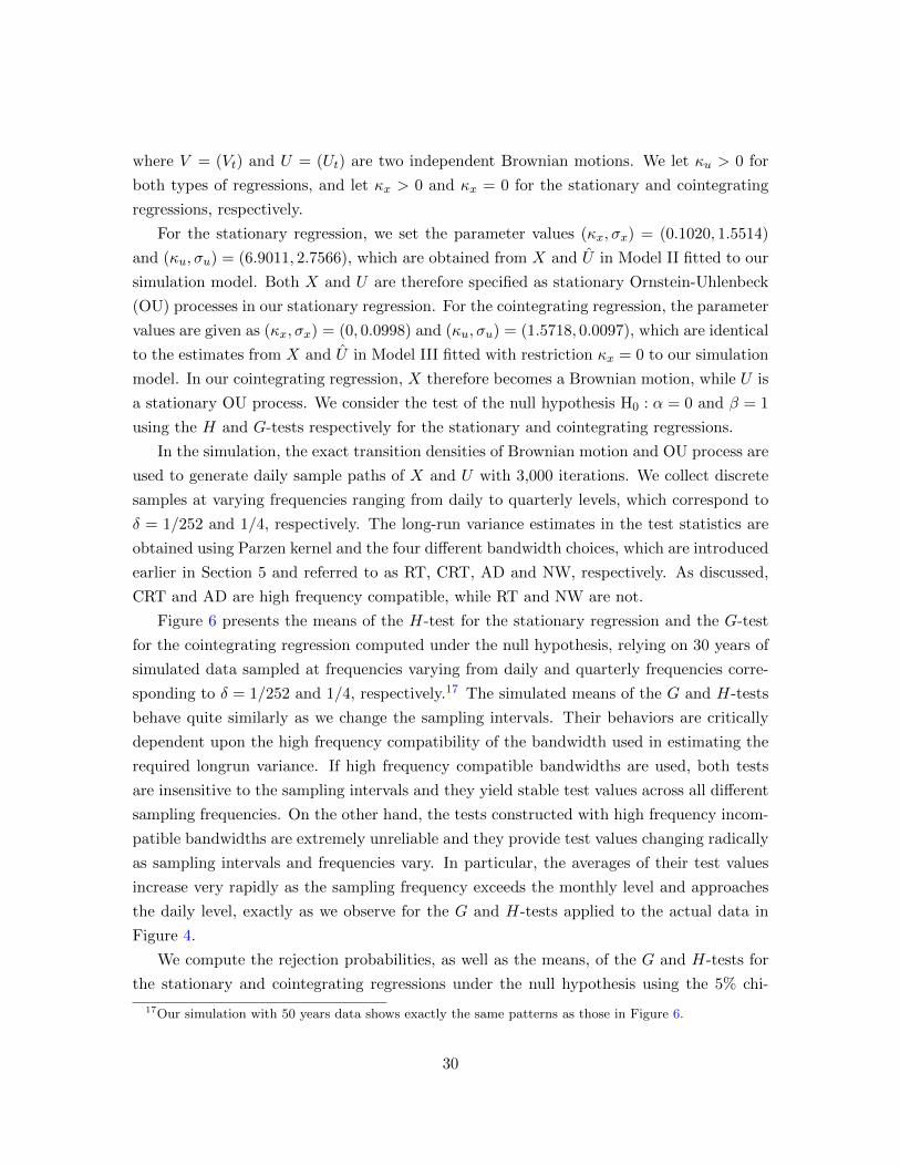
Figure 6 presents the means of the H-test for the stationary regression and the G-test

for the cointegrating regression computed under the null hypothesis, relying on 30 years of

simulated data sampled at frequencies varying from daily and quarterly frequencies corre-

sponding to δ = 1/252 and 1/4, respectively.17 The simulated means of the G and H-tests

behave quite similarly as we change the sampling intervals. Their behaviors are critically

dependent upon the high frequency compatibility of the bandwidth used in estimating the

required longrun variance. If high frequency compatible bandwidths are used, both tests

are insensitive to the sampling intervals and they yield stable test values across all different

sampling frequencies. On the other hand, the tests constructed with high frequency incom-

patible bandwidths are extremely unreliable and they provide test values changing radically

as sampling intervals and frequencies vary. In particular, the averages of their test values

increase very rapidly as the sampling frequency exceeds the monthly level and approaches

the daily level, exactly as we observe for the G and H-tests applied to the actual data in

Figure 4.

We compute the rejection probabilities, as well as the means, of the G and H-tests for

the stationary and cointegrating regressions under the null hypothesis using the 5% chi-

17Our simulation with 50 years data shows exactly the same patterns as those in Figure 6.

30

Fig. 6. Simulated Means of Robust Wald Tests

0 0.05 0.1 0.15 0.2 0.250

5

10

15

20

25

30

35

40

H: NWH: AD

0 0.05 0.1 0.15 0.2 0.250

5

10

15

20

25

30

35

40

H: RTH: CRT

0 0.05 0.1 0.15 0.2 0.250

5

10

15

20

G: NWG: AD

0 0.05 0.1 0.15 0.2 0.250

20

40

60

80

100

120

140

160

G: RTG: CRT

Notes: Presented are the simulated means of the H-test for the stationary regression (upper panel) and theG-test for the cointegrating regression (lower panel) computed under the null hypothesis. The bandwidthchoices are given by RT, CRT, AD and NW, and the sampling interval δ ranges from 1/252 (daily frequency)to 1/4 (quarterly frequency).

square critical value for T = 30 and 50. They are presented in Figure 7 in Appendix B. If

high frequency incompatible bandwidths are used, not only the means but also the rejection

probabilities of the tests become highly sensitive to the sampling frequency and increase

rapidly as the sampling interval decreases down below one month.18 In contrast, the rejec-

tion probabilities of the tests with high frequency compatible bandwidths are remarkably

stable across all sampling frequencies, and they tend closer to the nominal size of the tests

as T increases.

To see more clearly the effect of our double asymptotics relying on δ → 0 and T → ∞jointly, we set δ = (1/3)T−2 so that T changes simultaneously along with δ. Under this

setup, we simulate the means of the H and G-tests for the stationary and cointegrating

regressions under the null hypothesis, which is reported in Figure 8 in Appendix B. The

18The bandwidths given by RT and NW yield large size distortions even at relatively low frequencies forour stationary and cointegrating simulation models, respectively. However, they also have the tendency wedescribe here.

31

overall pattern of the frequency dependency remains the same as what we observe in Figure

6, which is obtained by changing only δ with T fixed. The only notable difference is that the

simulated means of the tests with high frequency compatible bandwidths, CRT and AD, now

show downward trends as the sampling interval gets smaller. As discussed, no such trends

appear when T is fixed. Therefore, we may conclude that the trends here are generated

not directly by varying δ but by T changing with δ. The downward trends emerging under

our double asymptotics just indicate that the tests have positive biases in our simulation

model when T is small. The simulated means of the tests with high frequency incompatible

bandwidths RT and NW behave similarly, regardless of T being fixed or varying with δ.

We conduct some additional simulations based on the models that can capture more

realistic features of the economic and financial series used in our empirical illustrations

presented in the previous section. Details of the additional simulation models are described

and the results obtained from these models are reported in Appendix C.

8. Conclusion

The Wald test is widely used to test for restrictions in regressions. However, the test is

extremely sensitive to the sampling frequency, and it is very likely that the test result

depends on the frequency of the samples we use for the test. This, of course, is highly

undesirable, since in most cases the sampling frequency has no bearing on the hypothesis

to be tested. The dependence of the Wald test on the sampling frequency is manifested

vividly in many time series regressions. In particular, when observations are used at high

frequency, the standard Wald test almost explodes and we are always led to reject the null

hypothesis no matter whether it is true or not. The problem, however, appears to have

long been either overlooked or neglected in the literature. Certainly, it has now become

increasingly more important as more economic and financial time series are collected and

made available at high frequencies.

In the paper, we develop a new continuous time framework and develop relevant asymp-

totics, relying on sampling interval δ and time span T jointly, to analyze various versions of

the Wald test in regressions with high frequency observations over long sample span. Our

framework accommodates both stationary and cointegrating regressions, and our asymp-

totics hold under mild regularity conditions. According to our asymptotic theory, the

standard Wald test is expected to diverge if δ → 0 fast enough relative to T →∞. This is

exactly what we observe in practice. The robust Wald tests, which use the longrun variance

estimates in place of the usual variance estimates, are expected to behave similarly unless

the bandwidths for their longrun variance estimates are appropriately chosen to be high

32

frequency compatible. The high frequency compatibility of a bandwidth ensures that the

resulting longrun variance estimate properly captures the clear and present serial correla-

tion at high frequency. Only when high frequency compatible bandwidths are used do the

robust Wald tests become valid and behave as expected under the null hypothesis.

References

Aıt-Sahalia, Y., Kimmel, R., 2007. Maximum likelihood estimation of stochastic volatilitymodels. Journal of Financial Economics 83 (2), 413–452.

Andrews, D. W. K., 1991. Heteroskedasticity and autocorrelation consistent covariancematrix estimation. Econometrica 59, 817–858.

Bernanke, B. S., 2020. The new tools of monetary policy. American Economic Review 110,943–983.

Chang, Y., Choi, Y., Kim, H., Park, J. Y., 2016. Evaluating factor pricing models usinghigh frequency panels. Quantitative Economics 7, 889–933.

Choi, Y., Jacewitz, S., Park, J. Y., 2016. A reexamination of stock return predictability.Journal of Econometrics 192, 168–189.

Granger, C. W. J., Newbold, P., 1974. Spurious regressions in econometrics. Journal ofEconometrics 2, 111–120.

Heston, S. L., 1993. A closed-form solution for options with stochastic volatility with appli-cations to bond and currency options. The Review of Financial Studies 6 (2), 327–343.

Jeong, M., Park, J. Y., 2011. Asymptotic theory of maximum likelihood estimator fordiffusion model, working Paper, Indiana University.

Jeong, M., Park, J. Y., 2014. Asymptotic theory of maximum likelihood estimator for jumpdiffusion model, working Paper, Indiana University.

Kanaya, S., Kim, J., Park, J. Y., 2018. On the modulus of continuity of brownian motion,working Paper, Indiana University.

Kim, J., Park, J. Y., 2017. Asymptotics for recurrent diffusions with application to highfrequency regression. Journal of Econometrics 196, 37–54.

Lu, Y., Park, J. Y., 2019. Estimation of longrun variance of continuous time stochasticprocess using discrete sample. Journal of Econometrics 210, 236–267.

Muller, U. K., 2005. Size and power of tests of stationarity in highly autocorrelated timeseries. Journal of Econometrics 128, 195–213.

Newey, W. K., West, K. D., 1994. Automatic lag selection in covariance matrix estimation.Review of Economic Studies 61, 631–653.

33

Perron, P., 1991a. A continuous-time approximation to the stationary first-order autore-gressive model. Econometric Theory 7, 236–252.

Perron, P., 1991b. A continuous-time approximation to the unstable first-order autoregres-sive model: The case without an intercept. Econometrica 59, 211–236.

Phillips, P. C. B., 1986. Understanding spurious regressions in econometrics. Journal ofEconometrics 33, 311–340.

Sun, Y., 2014. Let’s fix it: Fixed-b asymptotics versus small-b asymptotics in heteroskedas-ticity and autocorrelation robust inference. Journal of Econometrics 178, 659–677.

34

Appendices

A. Mathematical Proofs

Proof of Lemma 3.1 We may assume without loss of generality that Z is univariate bylooking at each component separately. Note that

1

T

∫ T

0Ztdt =

1

T

n∑i=1

∫ iδ

(i−1)δZtdt

1

n

n∑i=1

zi =1

T

n∑i=1

δZ(i−1)δ +δ

T(ZT − Z0),

from which it follows that

1

T

∫ T

0Ztdt−

1

n

n∑i=1

zi =1

T

n∑i=1

∫ iδ

(i−1)δ(Zt − Z(i−1)δ)dt+Op

(δ

Tsup

0≤t≤T|Zt|

).

However, we have

|Zt − Z(i−1)δ| ≤ |Zct − Zc(i−1)δ|+∑

(i−1)δ<s≤t

∆Zt

for all i = 1, . . . , n and t such that (i− 1)δ < t ≤ iδ. Consequently, we have∣∣∣∣∣ 1nn∑i=1

zi −1

T

∫ T

0Ztdt

∣∣∣∣∣ ≤ 1

T

n∑i=1

∫ iδ

(i−1)δ|Zt − Z(i−1)δ|dt+Op

(δ

Tsup

0≤t≤T|Zt|

)

and

1

T

n∑i=1

∫ iδ

(i−1)δ|Zt − Z(i−1)δ|dt ≤

1

T

n∑i=1

∫ iδ

(i−1)δ

|Zct − Zc(i−1)δ|+ ∑(i−1)δ<s≤t

|∆Zt|

dt

≤ 1

T

n∑i=1

∫ iδ

(i−1)δ

|Zct − Zc(i−1)δ|+ ∑(i−1)δ<s≤iδ

|∆Zt|

dt

≤

(sup|t−s|≤δ

|Zct − Zcs |

)+δ

T

∑0<t≤T

|∆Zt|

= Op

(∆δ,T (Z)

)+Op(δ),

and we may deduce the stated result immediately.

35

Proof of Theorem 4.1 Under Assumptions A and B, we have

1

n

n∑i=1

u2i =1

T

∫ T

0U2t dt+ op(1)→p σ

2

as δ → 0 and T →∞ with ∆δ,T (U) = o(1) as in Assumption D1 or D2.For the proof of part (a), we write

√T (β − β) =

(1

n

n∑i=1

xix′i

)−1 √δ√n

n∑i=1

xiui, (21)

and note that, under Assumptions A and C1, we have

1

n

n∑i=1

xix′i =

1

T

∫ T

0XtX

′tdt+ op(1)→p M > 0

√δ√n

n∑i=1

xiui =1√T

∫ T

0XtUtdt+ op(1)→d N(0,Π)

as δ → 0 and T →∞ satisfying Assumption D1, and that

σ2 =1

n

n∑i=1

u2i −1

T

(√δ√n

n∑i=1

uix′i

)(1

n

n∑i=1

xix′i

)−1(√δ√n

n∑i=1

xiui

)

=1

n

n∑i=1

u2i +Op(T−1).

Therefore, the stated results follow immediately.The proof of part (b) is completely analogous. We write

√TΛ′T (β − β) =

(1

n

n∑i=1

Λ−1T xix′iΛ−1′T

)−1 √δ√n

n∑i=1

Λ−1T xiui, (22)

and note that, under Assumptions A and C2, we have

1

n

n∑i=1

Λ−1T xix′iΛ−1′T =

1

T

∫ T

0Λ−1T XtX

′tΛ−1′dt+ op(1)

=

∫ 1

0XTt X

T ′t dt+ op(1)→d

∫ 1

0XtX

′t dt

36

and√δ√n

n∑i=1

Λ−1T xiui =1√T

∫ T

0Λ−1T XtUtdt+ op(1)

=

∫ 1

0XTt dU

Tt + op(1)→d

∫ 1

0Xt dU

t

as δ → 0 and T →∞ satisfying Assumption D2, and that

σ2 =1

n

n∑i=1

u2i −1

T

(√δ√n

n∑i=1

uix′iΛ−1′T

)(1

n

n∑i=1

Λ−1T xix′iΛ

1′T

)−1(√δ√n

n∑i=1

Λ−1T xiui

)

=1

n

n∑i=1

u2i +Op(T−1),

from which the stated results readily follow.

Proof of Lemma 4.2 Write

ρ− 1 =

n∑i=1

ui−1(ui − ui−1)

n∑i=1

u2i−1

. (23)

As shown earlier, we have n−1∑n

i=1 u2i−1 →p σ

2. Moreover, note that

ui−1 =1

2[(ui + ui−1)− (ui − ui−1)] ,

and therefore, we may deduce that

n∑i=1

ui−1(ui − ui−1) =1

2

[n∑i=1

(u2i − u2i−1)−n∑i=1

(ui − ui−1)2]

=1

2

(u2n − u20

)− 1

2

n∑i=1

(ui − ui−1)2,

which will be further analyzed subsequently.We have

(Uiδ − U(i−1)δ)2 = 2

∫ iδ

(i−1)δ(Ut− − U(i−1)δ)dU

ct +

([U c]iδ − [U c](i−1)δ

)+

∑(i−1)δ<t≤iδ

∆(Ut − U(i−1)δ)2, (24)

37

and

∆(Ut − U(i−1)δ)2 = (Ut − U(i−1)δ)

2 − (Ut− − U(i−1)δ)2

= (Ut − Ut−)(Ut + Ut− − 2U(i−1)δ)

= (Ut − Ut−)[(Ut − Ut−) + 2(Ut− − U(i−1)δ)

]= 2(Ut− − U(i−1)δ)∆Ut + (∆Ut)

2 (25)

for i = 1, . . . , n. Therefore, it follows from (24) and (25) that

n∑i=1

(Uiδ− − U(i−1)δ)2 = [U ]T + 2ZT , (26)

where Z = Zc + Zd with

ZcT =n∑i=1

∫ iδ

(i−1)δ(Ut− − U(i−1)δ)dU

ct

ZdT =n∑i=1

∑(i−1)δ<t≤iδ

(Ut− − U(i−1)δ)∆Ut.

Note that

[U ]T =n∑i=1

([U c]iδ − [U c](i−1)δ

)+∑

0<t≤T(∆Ut)

2

for any n and δ such that T = nδ. In what follows, we use

Ut− − U(i−1)δ = (U ct − U c(i−1)δ) +∑

(i−1)δ<s<t

∆Us, (27)

which holds for t, (i− 1)δ < t ≤ iδ, and all i = 1, . . . , n.To consider Zc, we write

Zc = Za + Zb, (28)

where

ZaT =

n∑i=1

∫ iδ

(i−1)δ(Ut− − U(i−1)δ)dAt

=n∑i=1

∫ iδ

(i−1)δ(U ct − U c(i−1)δ)dAt +

n∑i=1

∫ iδ

(i−1)δ

∑(i−1)δ<s<t

∆Us

dAt

38

and

ZbT =n∑i=1

∫ iδ

(i−1)δ(Ut− − U(i−1)δ)dBt

=n∑i=1

∫ iδ

(i−1)δ(U ct − U c(i−1)δ)dBt +

n∑i=1

∫ iδ

(i−1)δ

∑(i−1)δ<s<t

∆Us

dBt,

which we analyze subsequently. For Za, we have∣∣∣∣∣n∑i=1

∫ iδ

(i−1)δ(U ct − U c(i−1)δ)dAt

∣∣∣∣∣ ≤n∑i=1

∫ iδ

(i−1)δ|U ct − U c(i−1)δ||dAt|

≤ pTn∑i=1

∫ iδ

(i−1)δ|U ct − U c(i−1)δ|dt

≤ pT∆δ,T (U)

n∑i=1

∫ iδ

(i−1)δdt = Op

(pTT∆δ,T (U)

)and ∣∣∣∣∣∣

n∑i=1

∫ iδ

(i−1)δ

∑(i−1)δ<s<t

∆Us

dAt

∣∣∣∣∣∣ ≤n∑i=1

∫ iδ

(i−1)δ

∑(i−1)δ<s<t

|∆Us|

|dAt|≤ pT

n∑i=1

∑(i−1)δ<t≤iδ

|∆Ut|

∫ iδ

(i−1)δdt

= pT δ∑

0<t≤T|∆Ut| = Op(pTTδ),

from which it follows that

ZaT = Op(pTT∆δ,T (U)) +Op(pTTδ) = Op(pTT∆δ,T (U)), (29)

since δ = O(∆δ,T (U)).For Zb, it suffices to look at its quadratic variation, since it can be embedded into a

continuous martingale. However, we have

n∑i=1

∫ iδ

(i−1)δ(U ct − U c(i−1)δ)

2d[B]t ≤ qTn∑i=1

∫ iδ

(i−1)δ(U ct − U c(i−1)δ)

2dt

≤ qT∆2δ,T (U)

n∑i=1

∫ iδ

(i−1)δdt = Op

(qTT∆2

δ,T (U)).

39

Furthermore, it follows that

n∑i=1

∫ iδ

(i−1)δ

∑(i−1)δ<s<t

∆Us

2

d[B]t ≤ qTn∑i=1

∫ iδ

(i−1)δ

∑(i−1)δ<s<t

∆Us

2

dt,

and that

E

n∑i=1

∫ iδ

(i−1)δ

∑(i−1)δ<s<t

∆Us

2

dt

=n∑i=1

∫ iδ

(i−1)δE

∑(i−1)δ<s<t

∆Us

2

dt

=

n∑i=1

∫ iδ

(i−1)δ

∑(i−1)δ<s<t

E(∆Us)2

dt≤

n∑i=1

∑(i−1)δ<t≤iδ

E(∆Ut)2

∫ iδ

(i−1)δdt

= δ∑

0<t≤TE(∆Ut)

2 = O(δT ).

Therefore, we may deduce that

ZbT = Op

(√qTT∆δ,T (U)

)+Op

(√qTTδ

)= Op

(√qTT∆δ,T (U)

), (30)

since√δ = O(∆δ,T (U)). The order of Zc may now be easily obtained as

ZcT = Op (pTT∆δ,T (U)) +Op

(√qTT∆δ,T (U)

)= T

[Op (pT∆δ,T (U)) +Op

(√qT /T∆δ,T (U)

)](31)

from (29) and (30).To analyze Zd, we let

ZdT =

n∑i=1

∑(i−1)δ<t≤iδ

(Ut− − U(i−1)δ)∆Ut

=

n∑i=1

∑(i−1)δ<t≤iδ

(U ct − U c(i−1)δ)∆Ut +

n∑i=1

∑(i−1)δ<t≤iδ

∑(i−1)δ<s<t

∆Us

∆Ut

40

We have

E

n∑i=1

∑(i−1)δ<t≤iδ

(U ct − U c(i−1)δ)∆Ut

2

=

n∑i=1

∑(i−1)δ<t≤iδ

E(U ct − U c(i−1)δ)2E(∆Ut)

2

≤

[max1≤i≤n

sup(i−1)δ<t≤iδ

E(U ct − U c(i−1)δ)2

]n∑i=1

∑(i−1)δ<t≤iδ

E(∆Ut)2

=

[max1≤i≤n

sup(i−1)δ<t≤iδ

E(U ct − U c(i−1)δ)2

] ∑0<t≤T

E(∆Ut)2 = O

(T∆2

δ,T (U)). (32)

Moreover, we may easily deduce that

E

n∑i=1

∑(i−1)δ<t≤iδ

∑(i−1)δ<s<t

∆Us

∆Ut

2

=

n∑i=1

∑(i−1)δ<t≤iδ

E

∑(i−1)δ<s<t

∆Us

2

E(∆Ut)2

=n∑i=1

∑(i−1)δ<t≤iδ

∑(i−1)δ<s<t

E(∆Us)2

E(∆Ut)2

≤n∑i=1

∑(i−1)δ<s,t≤iδ

E(∆Us)2E(∆Ut)

2

≤n∑i=1

∑(i−1)δ<s,t≤iδ

E(∆Ut)4 =

∑0<t≤T

E(∆Ut)4 = O(T ). (33)

Therefore, it follows from (32) and (33) that

ZdT = Op

(√T∆δ,T (U)

)+Op(

√T ) = Op(

√T ) = op(T ) (34)

as δ → 0 and T →∞.

41

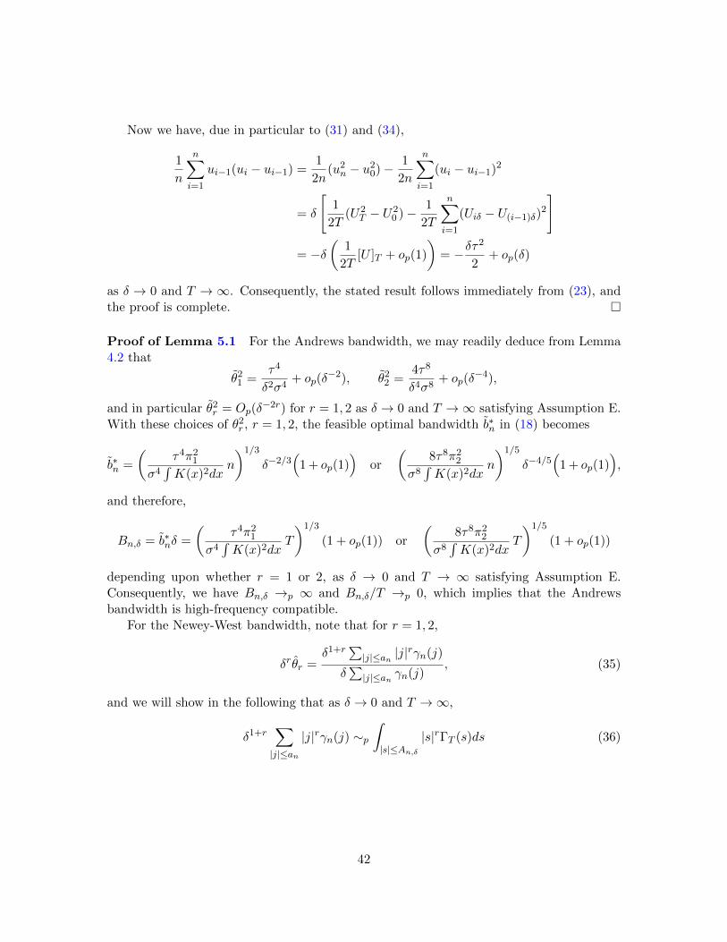
Now we have, due in particular to (31) and (34),

1

n

n∑i=1

ui−1(ui − ui−1) =1

2n(u2n − u20)−

1

2n

n∑i=1

(ui − ui−1)2

= δ

[1

2T(U2

T − U20 )− 1

2T

n∑i=1

(Uiδ − U(i−1)δ)2

]

= −δ(

1

2T[U ]T + op(1)

)= −δτ

2

2+ op(δ)

as δ → 0 and T → ∞. Consequently, the stated result follows immediately from (23), andthe proof is complete.

Proof of Lemma 5.1 For the Andrews bandwidth, we may readily deduce from Lemma4.2 that

θ21 =τ4

δ2σ4+ op(δ

−2), θ22 =4τ8

δ4σ8+ op(δ

−4),

and in particular θ2r = Op(δ−2r) for r = 1, 2 as δ → 0 and T →∞ satisfying Assumption E.

With these choices of θ2r , r = 1, 2, the feasible optimal bandwidth b∗n in (18) becomes

b∗n =

(τ4π21

σ4∫K(x)2dx

n

)1/3

δ−2/3(

1 + op(1))

or

(8τ8π22

σ8∫K(x)2dx

n

)1/5

δ−4/5(

1 + op(1)),

and therefore,

Bn,δ = b∗nδ =

(τ4π21

σ4∫K(x)2dx

T

)1/3

(1 + op(1)) or

(8τ8π22

σ8∫K(x)2dx

T

)1/5

(1 + op(1))

depending upon whether r = 1 or 2, as δ → 0 and T → ∞ satisfying Assumption E.Consequently, we have Bn,δ →p ∞ and Bn,δ/T →p 0, which implies that the Andrewsbandwidth is high-frequency compatible.

For the Newey-West bandwidth, note that for r = 1, 2,

δrθr =δ1+r

∑|j|≤an |j|

rγn(j)

δ∑|j|≤an γn(j)

, (35)

and we will show in the following that as δ → 0 and T →∞,

δ1+r∑|j|≤an

|j|rγn(j) ∼p∫|s|≤An,δ

|s|rΓT (s)ds (36)

42

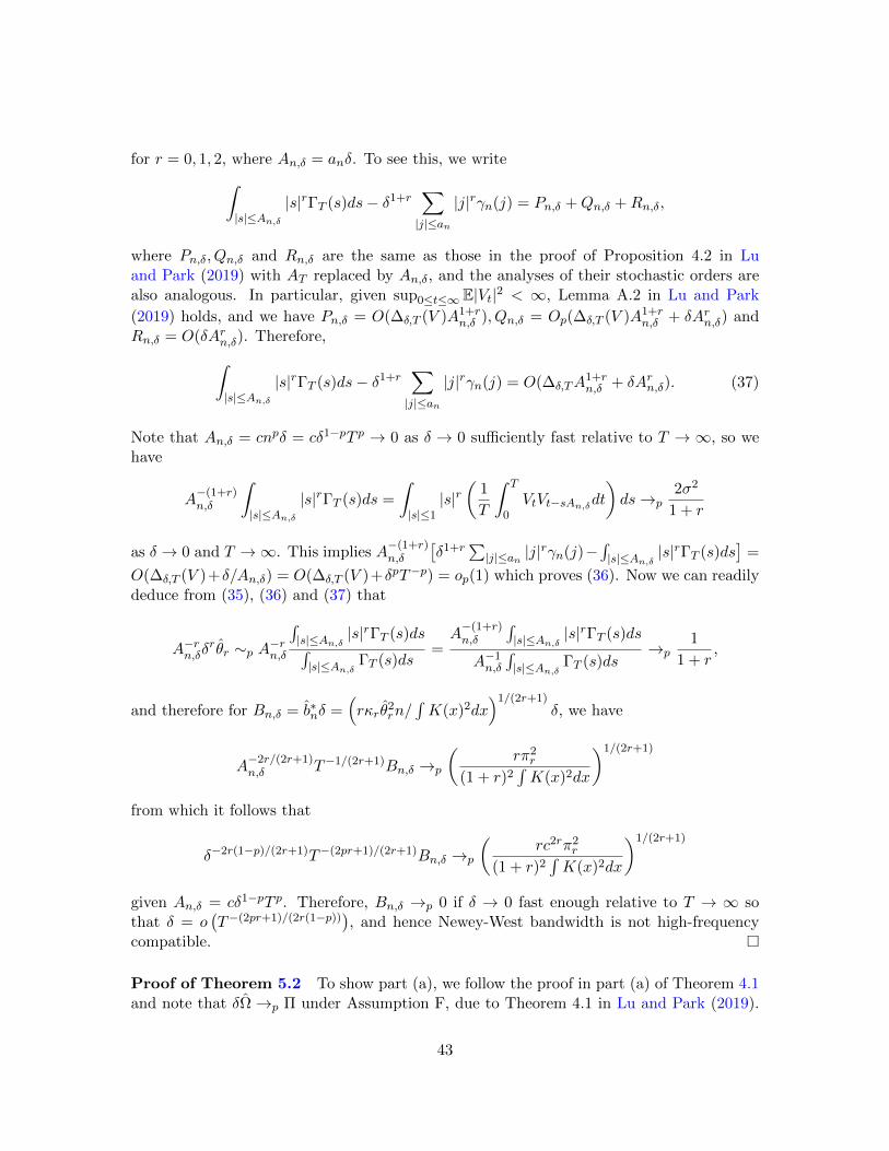
for r = 0, 1, 2, where An,δ = anδ. To see this, we write∫|s|≤An,δ

|s|rΓT (s)ds− δ1+r∑|j|≤an

|j|rγn(j) = Pn,δ +Qn,δ +Rn,δ,

where Pn,δ, Qn,δ and Rn,δ are the same as those in the proof of Proposition 4.2 in Luand Park (2019) with AT replaced by An,δ, and the analyses of their stochastic orders arealso analogous. In particular, given sup0≤t≤∞ E|Vt|2 < ∞, Lemma A.2 in Lu and Park

(2019) holds, and we have Pn,δ = O(∆δ,T (V )A1+rn,δ ), Qn,δ = Op(∆δ,T (V )A1+r

n,δ + δArn,δ) andRn,δ = O(δArn,δ). Therefore,∫

|s|≤An,δ|s|rΓT (s)ds− δ1+r

∑|j|≤an

|j|rγn(j) = O(∆δ,TA1+rn,δ + δArn,δ). (37)

Note that An,δ = cnpδ = cδ1−pT p → 0 as δ → 0 sufficiently fast relative to T → ∞, so wehave

A−(1+r)n,δ

∫|s|≤An,δ

|s|rΓT (s)ds =

∫|s|≤1|s|r

(1

T

∫ T

0VtVt−sAn,δdt

)ds→p

2σ2

1 + r

as δ → 0 and T →∞. This implies A−(1+r)n,δ

[δ1+r

∑|j|≤an |j|

rγn(j)−∫|s|≤An,δ |s|

rΓT (s)ds]

=

O(∆δ,T (V )+δ/An,δ) = O(∆δ,T (V )+δpT−p) = op(1) which proves (36). Now we can readilydeduce from (35), (36) and (37) that

A−rn,δδrθr ∼p A−rn,δ

∫|s|≤An,δ |s|

rΓT (s)ds∫|s|≤An,δ ΓT (s)ds

=A−(1+r)n,δ

∫|s|≤An,δ |s|

rΓT (s)ds

A−1n,δ∫|s|≤An,δ ΓT (s)ds

→p1

1 + r,

and therefore for Bn,δ = b∗nδ =(rκrθ

2rn/

∫K(x)2dx

)1/(2r+1)δ, we have

A−2r/(2r+1)n,δ T−1/(2r+1)Bn,δ →p

(rπ2r

(1 + r)2∫K(x)2dx

)1/(2r+1)

from which it follows that

δ−2r(1−p)/(2r+1)T−(2pr+1)/(2r+1)Bn,δ →p

(rc2rπ2r

(1 + r)2∫K(x)2dx

)1/(2r+1)

given An,δ = cδ1−pT p. Therefore, Bn,δ →p 0 if δ → 0 fast enough relative to T → ∞ sothat δ = o

(T−(2pr+1)/(2r(1−p))), and hence Newey-West bandwidth is not high-frequency

compatible.

Proof of Theorem 5.2 To show part (a), we follow the proof in part (a) of Theorem 4.1and note that δΩ →p Π under Assumption F, due to Theorem 4.1 in Lu and Park (2019).

43

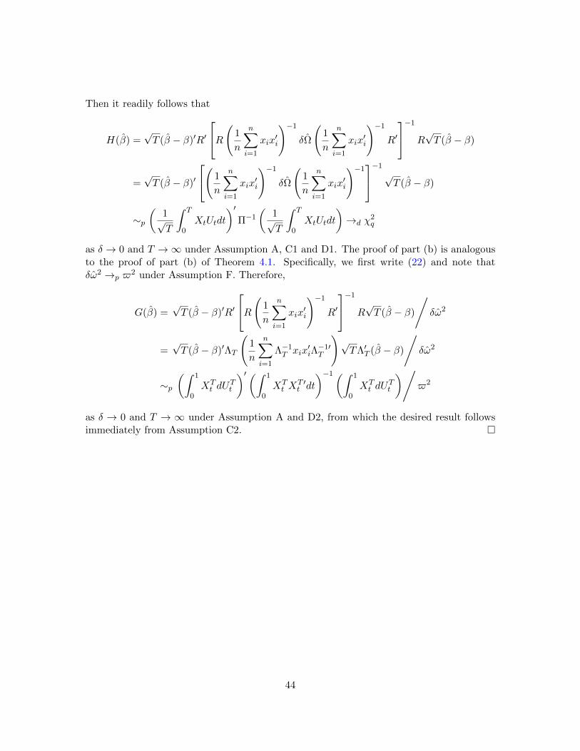
Then it readily follows that

H(β) =√T (β − β)′R′

R( 1

n

n∑i=1

xix′i

)−1δΩ

(1

n

n∑i=1

xix′i

)−1R′

−1R√T (β − β)

=√T (β − β)′

( 1

n

n∑i=1

xix′i

)−1δΩ

(1

n

n∑i=1

xix′i

)−1−1√T (β − β)

∼p(

1√T

∫ T

0XtUtdt

)′Π−1

(1√T

∫ T

0XtUtdt

)→d χ

2q

as δ → 0 and T →∞ under Assumption A, C1 and D1. The proof of part (b) is analogousto the proof of part (b) of Theorem 4.1. Specifically, we first write (22) and note thatδω2 →p $

2 under Assumption F. Therefore,

G(β) =√T (β − β)′R′

R( 1

n

n∑i=1

xix′i

)−1R′

−1R√T (β − β)

/δω2

=√T (β − β)′ΛT

(1

n

n∑i=1

Λ−1T xix′iΛ−1′T

)√TΛ′T (β − β)

/δω2

∼p(∫ 1

0XTt dU

Tt

)′(∫ 1

0XTt X

T ′t dt

)−1(∫ 1

0XTt dU

Tt

)/$2

as δ → 0 and T → ∞ under Assumption A and D2, from which the desired result followsimmediately from Assumption C2.

44

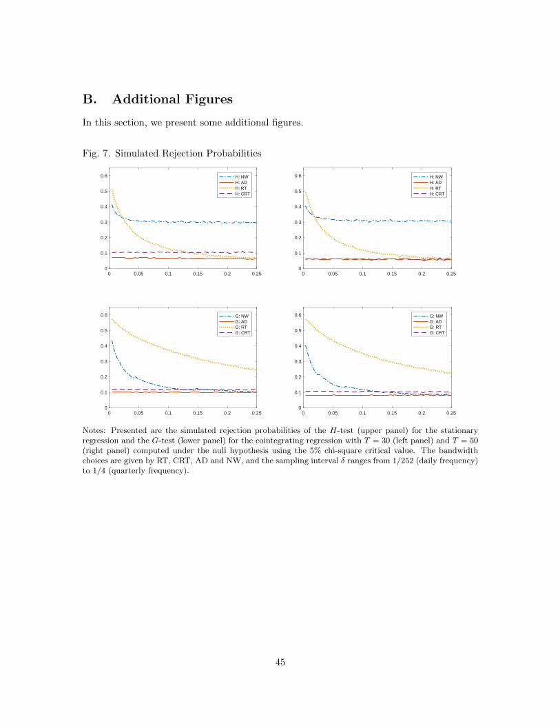
B. Additional Figures

In this section, we present some additional figures.

Fig. 7. Simulated Rejection Probabilities

0 0.05 0.1 0.15 0.2 0.250

0.1

0.2

0.3

0.4

0.5

0.6 H: NWH: ADH: RTH: CRT

0 0.05 0.1 0.15 0.2 0.250

0.1

0.2

0.3

0.4

0.5

0.6 G: NWG: ADG: RTG: CRT

0 0.05 0.1 0.15 0.2 0.250

0.1

0.2

0.3

0.4

0.5

0.6 H: NWH: ADH: RTH: CRT

0 0.05 0.1 0.15 0.2 0.250

0.1

0.2

0.3

0.4

0.5

0.6 G: NWG: ADG: RTG: CRT

Notes: Presented are the simulated rejection probabilities of the H-test (upper panel) for the stationaryregression and the G-test (lower panel) for the cointegrating regression with T = 30 (left panel) and T = 50(right panel) computed under the null hypothesis using the 5% chi-square critical value. The bandwidthchoices are given by RT, CRT, AD and NW, and the sampling interval δ ranges from 1/252 (daily frequency)to 1/4 (quarterly frequency).

45

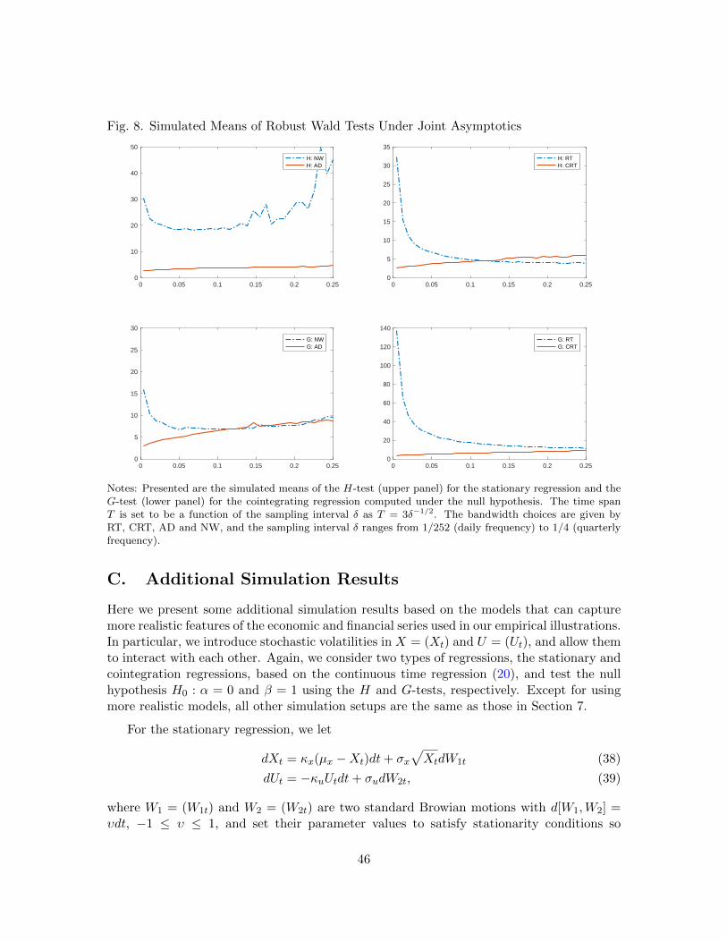
Fig. 8. Simulated Means of Robust Wald Tests Under Joint Asymptotics

0 0.05 0.1 0.15 0.2 0.250

10

20

30

40

50

H: NWH: AD

0 0.05 0.1 0.15 0.2 0.250

5

10

15

20

25

30

35

H: RTH: CRT

0 0.05 0.1 0.15 0.2 0.250

5

10

15

20

25

30

G: NWG: AD

0 0.05 0.1 0.15 0.2 0.250

20

40

60

80

100

120

140

G: RTG: CRT

Notes: Presented are the simulated means of the H-test (upper panel) for the stationary regression and theG-test (lower panel) for the cointegrating regression computed under the null hypothesis. The time spanT is set to be a function of the sampling interval δ as T = 3δ−1/2. The bandwidth choices are given byRT, CRT, AD and NW, and the sampling interval δ ranges from 1/252 (daily frequency) to 1/4 (quarterlyfrequency).

C. Additional Simulation Results

Here we present some additional simulation results based on the models that can capturemore realistic features of the economic and financial series used in our empirical illustrations.In particular, we introduce stochastic volatilities in X = (Xt) and U = (Ut), and allow themto interact with each other. Again, we consider two types of regressions, the stationary andcointegration regressions, based on the continuous time regression (20), and test the nullhypothesis H0 : α = 0 and β = 1 using the H and G-tests, respectively. Except for usingmore realistic models, all other simulation setups are the same as those in Section 7.

For the stationary regression, we let

dXt = κx(µx −Xt)dt+ σx√XtdW1t (38)

dUt = −κuUtdt+ σudW2t, (39)

where W1 = (W1t) and W2 = (W2t) are two standard Browian motions with d[W1,W2] =υdt, −1 ≤ υ ≤ 1, and set their parameter values to satisfy stationarity conditions so

46

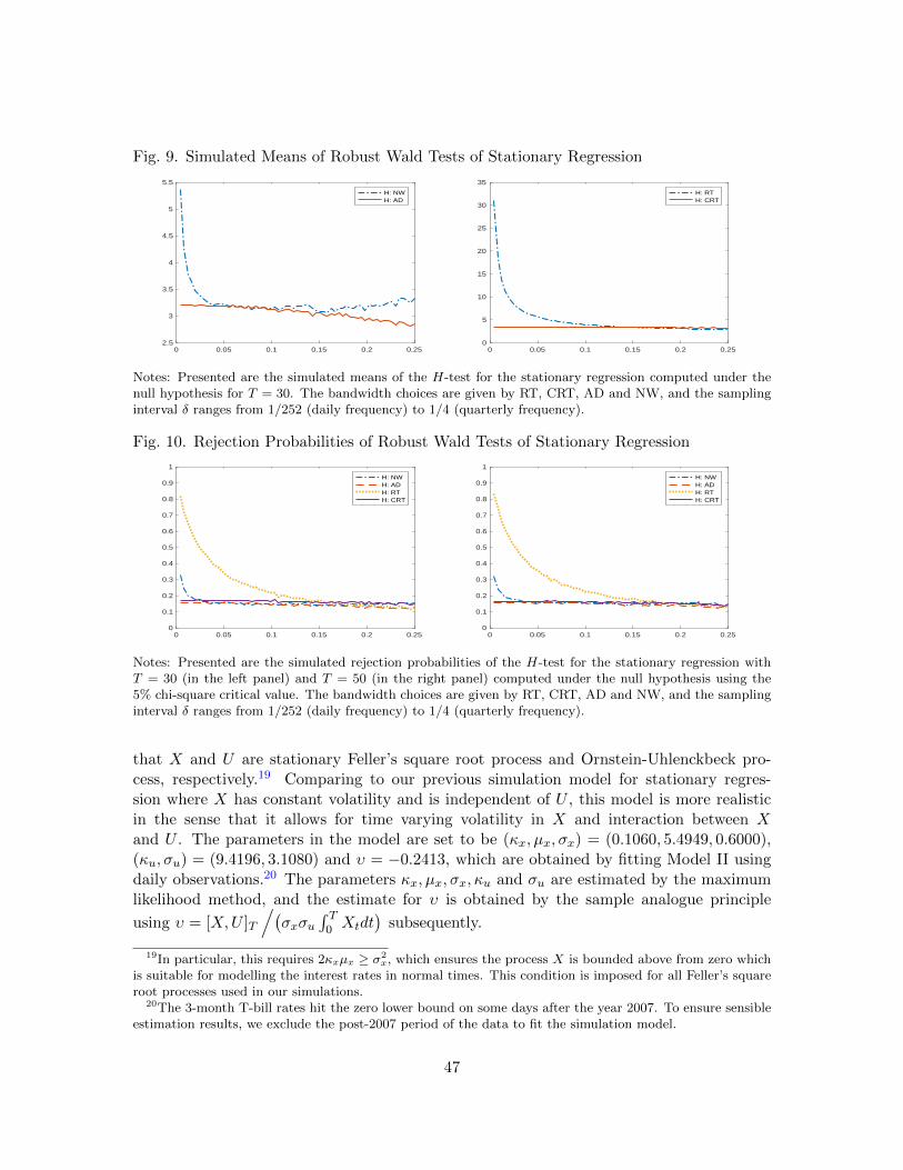
Fig. 9. Simulated Means of Robust Wald Tests of Stationary Regression

0 0.05 0.1 0.15 0.2 0.252.5

3

3.5

4

4.5

5

5.5

H: NWH: AD

0 0.05 0.1 0.15 0.2 0.250

5

10

15

20

25

30

35

H: RTH: CRT

Notes: Presented are the simulated means of the H-test for the stationary regression computed under thenull hypothesis for T = 30. The bandwidth choices are given by RT, CRT, AD and NW, and the samplinginterval δ ranges from 1/252 (daily frequency) to 1/4 (quarterly frequency).

Fig. 10. Rejection Probabilities of Robust Wald Tests of Stationary Regression

0 0.05 0.1 0.15 0.2 0.250

0.1

0.2

0.3

0.4

0.5

0.6

0.7

0.8

0.9

1

H: NWH: ADH: RTH: CRT

0 0.05 0.1 0.15 0.2 0.250

0.1

0.2

0.3

0.4

0.5

0.6

0.7

0.8

0.9

1

H: NWH: ADH: RTH: CRT

Notes: Presented are the simulated rejection probabilities of the H-test for the stationary regression withT = 30 (in the left panel) and T = 50 (in the right panel) computed under the null hypothesis using the5% chi-square critical value. The bandwidth choices are given by RT, CRT, AD and NW, and the samplinginterval δ ranges from 1/252 (daily frequency) to 1/4 (quarterly frequency).

that X and U are stationary Feller’s square root process and Ornstein-Uhlenckbeck pro-cess, respectively.19 Comparing to our previous simulation model for stationary regres-sion where X has constant volatility and is independent of U , this model is more realisticin the sense that it allows for time varying volatility in X and interaction between Xand U . The parameters in the model are set to be (κx, µx, σx) = (0.1060, 5.4949, 0.6000),(κu, σu) = (9.4196, 3.1080) and υ = −0.2413, which are obtained by fitting Model II usingdaily observations.20 The parameters κx, µx, σx, κu and σu are estimated by the maximumlikelihood method, and the estimate for υ is obtained by the sample analogue principle

using υ = [X,U ]T

/(σxσu

∫ T0 Xtdt

)subsequently.

19In particular, this requires 2κxµx ≥ σ2x, which ensures the process X is bounded above from zero which

is suitable for modelling the interest rates in normal times. This condition is imposed for all Feller’s squareroot processes used in our simulations.

20The 3-month T-bill rates hit the zero lower bound on some days after the year 2007. To ensure sensibleestimation results, we exclude the post-2007 period of the data to fit the simulation model.

47

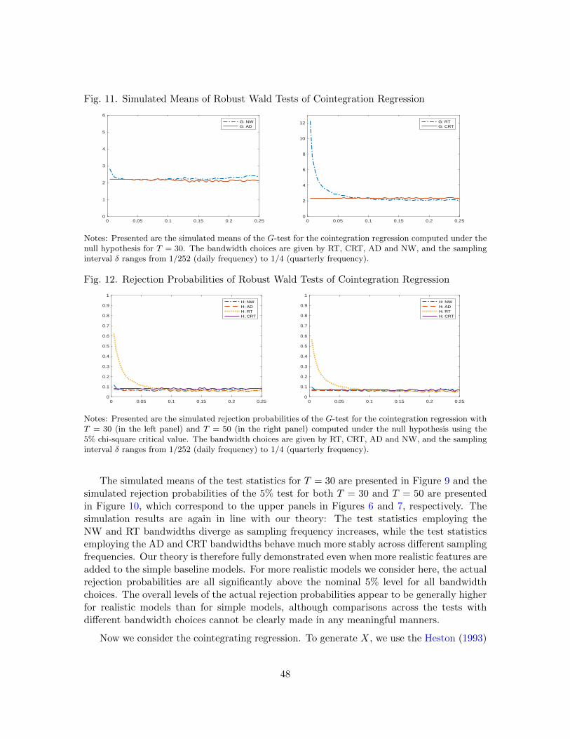
Fig. 11. Simulated Means of Robust Wald Tests of Cointegration Regression

0 0.05 0.1 0.15 0.2 0.250

1

2

3

4

5

6

G: NWG: AD

0 0.05 0.1 0.15 0.2 0.250

2

4

6

8

10

12 G: RTG: CRT

Notes: Presented are the simulated means of the G-test for the cointegration regression computed under thenull hypothesis for T = 30. The bandwidth choices are given by RT, CRT, AD and NW, and the samplinginterval δ ranges from 1/252 (daily frequency) to 1/4 (quarterly frequency).

Fig. 12. Rejection Probabilities of Robust Wald Tests of Cointegration Regression

0 0.05 0.1 0.15 0.2 0.250

0.1

0.2

0.3

0.4

0.5

0.6

0.7

0.8

0.9

1

H: NWH: ADH: RTH: CRT

0 0.05 0.1 0.15 0.2 0.250

0.1

0.2

0.3

0.4

0.5

0.6

0.7

0.8

0.9

1

H: NWH: ADH: RTH: CRT

Notes: Presented are the simulated rejection probabilities of the G-test for the cointegration regression withT = 30 (in the left panel) and T = 50 (in the right panel) computed under the null hypothesis using the5% chi-square critical value. The bandwidth choices are given by RT, CRT, AD and NW, and the samplinginterval δ ranges from 1/252 (daily frequency) to 1/4 (quarterly frequency).

The simulated means of the test statistics for T = 30 are presented in Figure 9 and thesimulated rejection probabilities of the 5% test for both T = 30 and T = 50 are presentedin Figure 10, which correspond to the upper panels in Figures 6 and 7, respectively. Thesimulation results are again in line with our theory: The test statistics employing theNW and RT bandwidths diverge as sampling frequency increases, while the test statisticsemploying the AD and CRT bandwidths behave much more stably across different samplingfrequencies. Our theory is therefore fully demonstrated even when more realistic features areadded to the simple baseline models. For more realistic models we consider here, the actualrejection probabilities are all significantly above the nominal 5% level for all bandwidthchoices. The overall levels of the actual rejection probabilities appear to be generally higherfor realistic models than for simple models, although comparisons across the tests withdifferent bandwidth choices cannot be clearly made in any meaningful manners.

Now we consider the cointegrating regression. To generate X, we use the Heston (1993)

48

model (see also in Aıt-Sahalia and Kimmel (2007)), which is often used for modelling thelog stock index price process X jointly with the spot variance process V x as

d

[Xt

V xt

]=

[(r − d) + bV x

t

κx(µx − V xt )

]dt+

[√(1− υ2)V x

t υ√V xt

0 σx√V xt

]d

[W x

1t

W x2t

], (40)

where r is the risk-free interest rate, d is the dividend yield of the stock index, and W x =(W x

1 ,Wx2 ) is standard bivariate Brownian motion. For simplicity, we let r and d be constant.

Note that the spot variance process V x is assumed to follow a stationary Feller’s square rootprocess. Moreover, −1 < υ < 0 represents the leverage effect, i.e., the negative correlationbetween the shocks to the stock price and its volatility. The parameter values used in oursimulations are obtained from X in Model IV fitted to the model in (40) using the methodproposed by Aıt-Sahalia and Kimmel (2007). In particular, we set κx = 3, µx = 0.1, σx =0.25, υ = −0.8 and b = 6.06. The values of r and d are set 2% and 1.5%, respectively.

For U , we also use a stochastic volatility model. We specify U jointly with its spotvariance process V u as

d

[UtV ut

]=

[−κUt

κu(µu − V ut )

]dt+

[√V ut 0

0 σu√V ut

]d

[W u

1t

W u2t

], (41)

where W u = (W u1 ,W

u2 ) is standard bivariate Brownian motion. Note that U is specified as

a zero-mean stationary process having stochastic volatility generated as the Feller’s squareroot process V u. The parameter values used in our simulations are from U in Model IV,estimated and fitted to the model in (41). In particular, we set κ = 20, κu = 2, µu = 0.0002and σu = 0.008. Each simulated data series is initialized with the instantaneous volatilitiesV x0 and V u

0 at their unconditional means, the log stock index price X0 at ln(100), and theerror process U0 at 0. The initial 500 observations are discarded to remove any potentialinitialization effects.

The simulated means of the test statistics for T = 30 are presented in Figure 11, and thesimulated rejection probabilities of the 5% test for both T = 30 and T = 50 are presentedin Figure 12. They correspond to the lower panels in Figures 6 and 7. Once again, oursimulation results are consistent with our theory. They clearly demonstrate that the testsemploying the NW and RT bandwidths tend to diverge as sampling frequency increases,whereas the tests employing the AD and CRT bandwidths do not show such a tendency.Such contrast in the limit behaviors of the tests is much more conspicuous between thetests with the RT and CRT bandwidths, than between the tests with the NW and ADbandwidths. We do not attempt to further interpret the details of our simulation resultshere. There are many aspects of our simulation models, including their parameter values,that could affect the performances of the tests with different choices of bandwidths indifferent ways, and we do not believe that we can unravel the individual effect of any oneof those aspects on the test with a particular choice of bandwidth.

49