1

Supporting information:

Understanding nitrate formation in a world with less sulfate.

1

Petros Vasilakos1, Armistead Russell2, Rodney Weber3, and Athanasios Nenes1,3,4,5†

1 School of Chemical and Biomolecular Engineering, Georgia Institute of Technology, Atlanta,

Georgia, 30332, USA

2School of Civil and Environmental Engineering, Georgia Institute of Technology, Atlanta,

Georgia, 30332, USA

3School of Earth and Atmospheric Sciences, Georgia Institute of Technology, Atlanta, Georgia,

30332, USA

4Institute of Chemical Engineering Sciences, Foundation for Research and Technology-Hellas,

Patras, GR 26504, Greece

5Institute for Environmental Research and Sustainable Development, National Observatory of

Athens, Palea Penteli, GR 15236, Greece

†Corresponding Author: A. Nenes (athanasios.nenes@gatech.edu)

2

3

2

4

Figure S1 - Yearly averaged predicted concentration fields of (a) 2001 NH4, (b) 2011 NH4, (c) 5

2001 SO4 (d) 2011 SO4, (e) 2001 NO3, (f) 2011 NO3. Color scales between years are kept the same 6

for parity, except for sulfate, due to its drastic reduction during the decade 7

8

Table S1 – Yearly domain averages and standard deviations for ammonium, sulfate and nitrate 9

in μg m-3 for 2001 & 2011 10

2001 NH4 SO4 NO3 2011 NH4 SO4 NO3

Domain

average 0.42 1.67 1.28

Domain

average 0.40 1.20 1.27

St.dev 0.47 1.02 1.43 St.dev 0.45 0.63 1.48

11

12

3

13

Figure S2 - Seasonally averaged pH over CONUS for the winter (January) of (a) 2001, (b) 2011, 14

the summer (July) of (d) 2001, (e) 2011. Panel (c) is difference between the simulation years for 15

the winter, and (f) is the difference for the summer. As in Figure 3, the study domain is highlighted. 16

17

4

18 Figure S3 – RH diurnal profiles for May (a), August (b), September (c) and November (d) at 19

JST/RS/GT, July (e) and December (f) at YRK and for the SOAS campaign period (g). Blue line 20

is the CMAQ predicted RH for 2001 and 2011, while the red line represents the measurements 21

22

5

23

Figure S4 – Total NVC diurnal profiles (Na+, Ca+2, K+ and Mg+2) for May (a), August (b), 24

September (c) and November (d) at JST/RS/GT, July (e) and December (f) at YRK and for the 25

SOAS campaign period (g). Blue and red lines are the CMAQ predicted NVCs for 2001 and 2011 26

respectively, while the shaded areas are one model standard deviation. 27

28

6

29

Figure S5 – pH diurnal profiles when not accounting for NVCs, for May (a), August (b), 30

September (c) and November (d) at JST/RS/GT, July (e) and December (f) at YRK and for the 31

SOAS campaign period (g). Blue and red lines are the CMAQ predicted pH for 2001 and 2011 32

respectively, while the shaded areas are one model standard deviation. Green line represents the 33

measurements and the shades area is standard error. 34

35

7

36

Figure S6 – pH diurnal profiles with assimilated RH when NVCs are included in the calculations, 37

for November at JST/RS/GT (a), the SOAS period (b) and July at YRK (c), and when NVCs are 38

not included for November at JST/RS/GT (d), the SOAS period (e) and July at YRK (f). Blue and 39

red lines are the CMAQ predicted pH for 2001 and 2011 respectively, while the shaded areas are 40

one model standard deviation. Green line represents the measurements and the shades area is 41

standard error. 42

43

8

Organic acids and pH 44

To determine the impact of organic compounds on acidity we tested a variety of scenarios 45

for our CMAQ results at the SEARCH sites, using the web-version of the Extended Aerosol 46

Inorganics Model (E-AIM) model (Wexler & Clegg 2002, Friese & Ebel 2010, Clegg et al. 1992) 47

(http://www.aim.env.uea.ac.uk/aim/aim.php). More specifically, we assumed that a set amount 48

(25 or 50% on a mole basis) of either oxalic, maleic, succinic or malonic acid already exists in the 49

aerosol phase but is not accounted for. Given the constant reductions in sulfate, we also tested the 50

potential of sulfate to be substituted by the same organics. To avoid the potential biases that NVCs 51

can incur on simulations, all runs were conducted without them. E-AIM was run using the 52

comprehensive Model IV configuration, in metastable mode. The baseline case that we used, was 53

the average composition, temperature and RH across all sites. 54

When comparing the total aerosol partitioning (particle to gas) for each SEARCH site 55

between ISORROPIA and E-AIM, they compare favorably, displaying an almost linear correlation 56

between the two (Fig. S7). For the low temperatures of December in Yorkville (T̿ ≤ 10oC) E-AIM 57

predicts a near complete absence of gas phase, in contrast to ISORROPIA, which is attributed to 58

the difference of how the activity coefficients are calculated between the two models (Wexler & 59

Clegg 2002, Friese & Ebel 2010, Clegg et al. 1992). Acidity between the two models differs, but 60

both predict sufficiently low values for pH for all sites (Table S2). 61

Initially, an amount of 25 or 50% of additional oxalic acid on a mole basis was added to 62

the baseline case, and then the pH was compared (Table S2). We find that for the cases presented 63

in this study, addition of organic compounds to the model did not have a significant impact on 64

acidity when compared to the baseline run, apart from the cases where RH was higher than 80% 65

and the mole fraction of organic acids in the aqueous phase is greater than 25%. pH remains rather 66

insensitive to the addition of oxalic acid for most cases, apart from the case that has the highest 67

RH=0.8, and subsequently the highest amount of liquid water. For all other cases, most of oxalic 68

acid partitions to the gas phase and its impact is negligible. Similarly, when other organic acids 69

are tested against the baseline, under the same conditions (maleic, succinic, malonic), they incur 70

a maximum 4% change on pH (Table S3). 71

For the substitution tests with oxalic acid, removal of sulfate from the system rapidly 72

decreases the amount of total water in the particulate phase (Fig. S8). This leads to the partitioning 73

of organics to the gas phase (Fig. S8), abating their impact on pH, since the relative composition 74

on a mole fraction basis remains largely the same. 75

The above analysis demonstrates that, for the cases presented in this paper, organics do not 76

have an appreciable impact on pH when only one liquid phase exists. Allowing more than one 77

liquid phase of different compositions to form, can still potentially impact pH (Pye et al. 2018). 78

9

79

80

Figure S7 –Nitrate (black) and total (red) particle-to-gas partitioning predicted between E-AIM 81

and ISORROPIA. 82

83

84

85

86

87

88

89

90

10

Table S2 – ISORROPIA, E-AIM and E-AIM with an additional 25 and 50% oxalic acid 91

predicted pH for all sites. 92

ISORROPIA

PH

pH

EAIM

pH 25%

OXALIC

pH 50%

OXALIC

-0.22 0.81 0.82 0.83

-0.30 0.92 0.92 0.91

0.55 1.31 1.32 1.25

-0.04 0.91 0.90 0.83

-0.01 0.55 0.55 0.55

0.07 0.34 0.34 0.34

0.14 0.53 0.53 0.52

-0.46 0.91 0.71 0.57

1.49 1.00 1.10 1.18

93

94

95

Figure S8 –Comparison of predicted particle-to-gas partitioning of oxalic acid (red) and total 96

water (black) between E-AIM and ISORROPIA as a function of sulfate substitution to oxalic 97

acid. 98

99

11

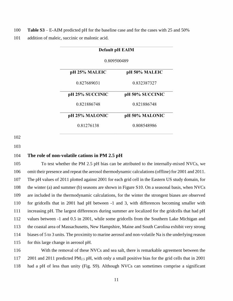
Table S3 – E-AIM predicted pH for the baseline case and for the cases with 25 and 50% 100

addition of maleic, succinic or malonic acid. 101

Default pH EAIM

0.809500489

pH 25% MALEIC pH 50% MALEIC

0.827689031 0.832387327

pH 25% SUCCINIC pH 50% SUCCINIC

0.821886748 0.821886748

pH 25% MALONIC pH 50% MALONIC

0.81276138 0.808548986

102

103

The role of non-volatile cations in PM 2.5 pH 104

To test whether the PM 2.5 pH bias can be attributed to the internally-mixed NVCs, we 105

omit their presence and repeat the aerosol thermodynamic calculations (offline) for 2001 and 2011. 106

The pH values of 2011 plotted against 2001 for each grid cell in the Eastern US study domain, for 107

the winter (a) and summer (b) seasons are shown in Figure S10. On a seasonal basis, when NVCs 108

are included in the thermodynamic calculations, for the winter the strongest biases are observed 109

for gridcells that in 2001 had pH between -1 and 3, with differences becoming smaller with 110

increasing pH. The largest differences during summer are localized for the gridcells that had pH 111

values between -1 and 0.5 in 2001, while some gridcells from the Southern Lake Michigan and 112

the coastal area of Massachusetts, New Hampshire, Maine and South Carolina exhibit very strong 113

biases of 5 to 3 units. The proximity to marine aerosol and non-volatile Na is the underlying reason 114

for this large change in aerosol pH. 115

With the removal of these NVCs and sea salt, there is remarkable agreement between the 116

2001 and 2011 predicted PM2.5 pH, with only a small positive bias for the grid cells that in 2001 117

had a pH of less than unity (Fig. S9). Although NVCs can sometimes comprise a significant 118

12

portion of PM2.5, as it was the case for the SOAS campaign (Allen et al. 2015, Bondy et al. 2017), 119

on average they should not be a major constituent of PM2.5 (Guo et al. 2015) over the Eastern 120

US, which is indicative of a portion of coarse mode dust being distributed to the smaller sized 121

aerosol in CMAQ , contrary to what has thus far been observed (Foroutan et al. 2017). While the 122

dust emissions were the same between the 2001 and 2011 simulations, given the same meteorology 123

for these years, and the fact that they were not scaled up/down in our model emissions, their impact 124

became much larger in 2011 due to the reductions in sulfate. NVCs on average account for 0.39 125

μg m-3 of CMAQ PM2.5 both in 2011 and 2001 over the Eastern US, which a factor of 4 higher 126

than the measured PM1 NVCs during the WINTER campaign (Guo et al. 2016). There is no bias 127

for the gridcells near coastal areas for this case, indicating that these areas were strongly affected 128

by the abundance of sea salt aerosol in fine PM. 129

To verify this finding, we compared observations of NVCs from the Metrohm Monitor for 130

AeRosol and Gases (MARGA) for the SOAS campaign, as well as the SEARCH and CSN sites, 131

to CMAQ results. The average mass of modelled NVCs for these sites is 0. 56 μg m-3, when 132

compared to 0.14 μg m-3 for the SEARCH/CSN average, indicating a factor of 4 overestimation, 133

mainly from crustal elements (K+, Ca+2 and Mg+2), further corroborated by the findings of Pye et 134

al. 2018, where the same comparison was carried out. 135

136

137

Table S4 – Comparison of NVCs (μg m-3) between simulation results for the 3 SEARCH 138

sites, and the measurements provided in Allen et al. 2015 and Pye et al. 2018 139

140

Na Mg K Ca Total NVCs

JST AUG 0.024 0.033 0.135 0.462 0.653

JST MAY 0.039 0.040 0.146 0.473 0.697

JST NOV 0.053 0.049 0.192 0.533 0.826

JST SEP 0.029 0.038 0.155 0.450 0.671

YRK DEC 0.052 0.044 0.184 0.412 0.692

YRK JUL 0.014 0.010 0.063 0.098 0.185

CSN 0.050 0.000 0.060 0.030 0.140

SEARCH 0.050 - 0.060 0.030 0.140

SOAS 0.032 0.007 0.071 0.083 0.193

MARGA 0.074 0.010 0.045 0.047 0.175

141

13

142

Figure S9 - Scatter plots of ISORROPIA predicted pH over the Eastern US study domain, for the 143

winter (a) and summer (b), with and without NVCs. 144

145

Figure S10 – Difference in nitrate over the Eastern US, between ISORROPIA predicted nitrate 146

when NVCs are included in calculations, and when they are excluded, for July (a) and January (b) 147

of 2011. 148

149

14

150

Figure S11 – Difference in predicted nitrate over the Eastern US between 2011 and 2001 when 151

NVCs are included in calculations (a), and when they are excluded (b). 152

153

154

15

References 155

Allen, H. M., D. C. Draper, B. R. Ayres, A. Ault, A. Bondy, S. Takahama, R. L. Modini, K. 156

Baumann, E. Edgerton, C. Knote, A. Laskin, B. Wang, and J. L. Fry (2015), Influence of crustal 157

dust and sea spray supermicron particle concentrations and acidity on inorganic NO3‐ aerosol 158

during the 2013 Southern Oxidant and Aerosol Study, Atmospheric Chemistry and Physics, 159

15(18), 10669‐10685. 160

Bondy, A. L., B. Wang, A. Laskin, R. L. Craig, M. V. Nhliziyo, S. Bertman, K. A. Pratt, P. B. 161

Shepson, and A. P. Ault (2017), Inland Sea Spray Aerosol Transport and Incomplete Chloride 162

Depletion: Varying Degrees of Reactive Processing Observed during SOAS, Environmental 163

Science & Technology. 164

Clegg, S. L., Pitzer, K. S., and Brimblecombe, P., Thermodynamics of multicomponent, miscible, 165

ionic solutions. II. Mixtures including unsymmetrical electrolytes. J. Phys. Chem. 96, 9470-9479, 166

DOI: 10.1021/j100202a074, 1992 167

Foroutan, H., J. Young, S. Napelenok, L. Ran, K. W. Appel, R. C. Gilliam, and J. E. Pleim (2017), 168

Development and evaluation of a physics-based windblown dust emission scheme implemented 169

in the CMAQ modeling system, J. Adv. Model. Earth Syst., 9, 585–608, 170

doi:10.1002/2016MS000823. 171

Friese, E. and Ebel, A., Temperature dependent thermodynamic model of the system H+ - NH4+ 172

- Na+ - SO42− - NO3− - Cl− - H2O. J. Phys. Chem. A, 114, 11595-11631, DOI: 173

10.1021/jp101041j, 2010 174

Guo, H., Sullivan, A.P., Campuzano-Jost, P., Schroder, J.C., Lopez-Hilfiger, F.D., Dibb, J.E., 175

Jimenez, J.L., Thornton, J.A, Brown, S.S., Nenes, A., and Weber, R.J. (2016) Fine particle pH and 176

the partitioning of nitric acid during winter in the northeastern United States, J.Geoph.Res., 121, 177

doi:10.1002/2016JD025311 178

Guo, H., Xu, L., Bougiatioti, A., Cerully, K. M., Capps, S. L., Hite Jr., J. R., Carlton, A. G., Lee, 179

S.-H., Bergin, M. H., Ng, N. L., Nenes, A., and Weber, R. J.: Fine-particle water and pH in the 180

16

southeastern United States, Atmos. Chem. Phys., 15, 5211-5228, doi:10.5194/acp-15-5211-2015, 181

2015. 182

Pye, H. O. T., Zuend, A., Fry, J. L., Isaacman-VanWertz, G., Capps, S. L., Appel, K. W., Foroutan, 183

H., Xu, L., Ng, N. L., and Goldstein, A. H.: Coupling of organic and inorganic aerosol systems 184

and the effect on gas–particle partitioning in the southeastern US, Atmos. Chem. Phys., 18, 357-185

370, https://doi.org/10.5194/acp-18-357-2018, 2018. 186

Wexler, A. S., and S. L. Clegg, Atmospheric aerosol models for systems including the ions H+, 187

NH4+, Na+, SO42−, NO3−, Cl−, Br−, and H2O, J. Geophys. Res., 107(D14), DOI: 188

10.1029/2001JD000451, 2002, http://www.aim.env.uea.ac.uk/aim/aim.php 189

190

191