Understanding Neural Networks Through Deep Visualization

Jason Yosinski YOSINSKI@CS.CORNELL.EDU

Cornell University

Jeff Clune JEFFCLUNE@UWYO.EDUAnh Nguyen ANGUYEN8@UWYO.EDU

University of Wyoming

Thomas Fuchs FUCHS@CALTECH.EDU

Jet Propulsion Laboratory, California Institute of Technology

Hod Lipson HOD.LIPSON@CORNELL.EDU

Cornell University

Abstract

Recent years have produced great advances intraining large, deep neural networks (DNNs), in-cluding notable successes in training convolu-tional neural networks (convnets) to recognizenatural images. However, our understanding ofhow these models work, especially what compu-tations they perform at intermediate layers, haslagged behind. Progress in the field will befurther accelerated by the development of bet-ter tools for visualizing and interpreting neuralnets. We introduce two such tools here. Thefirst is a tool that visualizes the activations pro-duced on each layer of a trained convnet as itprocesses an image or video (e.g. a live web-cam stream). We have found that looking at liveactivations that change in response to user inputhelps build valuable intuitions about how con-vnets work. The second tool enables visualizingfeatures at each layer of a DNN via regularizedoptimization in image space. Because previousversions of this idea produced less recognizableimages, here we introduce several new regular-ization methods that combine to produce qualita-tively clearer, more interpretable visualizations.Both tools are open source and work on a pre-trained convnet with minimal setup.

Published in the Deep Learning Workshop, 31 st InternationalConference on Machine Learning, Lille, France, 2015. Copyright2015 by the author(s).

1. IntroductionThe last several years have produced tremendous progressin training powerful, deep neural network models that areapproaching and even surpassing human abilities on a vari-ety of challenging machine learning tasks (Taigman et al.,2014; Schroff et al., 2015; Hannun et al., 2014). A flagshipexample is training deep, convolutional neural networks(CNNs) with supervised learning to classify natural images(Krizhevsky et al., 2012). That area has benefitted from thecombined effects of faster computing (e.g. GPUs), bettertraining techniques (e.g. dropout (Hinton et al., 2012)), bet-ter activation units (e.g. rectified linear units (Glorot et al.,2011)), and larger labeled datasets (Deng et al., 2009; Linet al., 2014).

While there has thus been considerable improvements inour knowledge of how to create high-performing architec-tures and learning algorithms, our understanding of howthese large neural models operate has lagged behind. Neu-ral networks have long been known as “black boxes” be-cause it is difficult to understand exactly how any particu-lar, trained neural network functions due to the large num-ber of interacting, non-linear parts. Large modern neuralnetworks are even harder to study because of their size;for example, understanding the widely-used AlexNet DNNinvolves making sense of the values taken by the 60 mil-lion trained network parameters. Understanding what islearned is interesting in its own right, but it is also onekey way of further improving models: the intuitions pro-vided by understanding the current generation of modelsshould suggest ways to make them better. For example,the deconvolutional technique for visualizing the featureslearned by the hidden units of DNNs suggested an archi-tectural change of smaller convolutional filters that led to

state of the art performance on the ImageNet benchmark in2013 (Zeiler & Fergus, 2013).

We also note that tools that enable understanding will es-pecially benefit the vast numbers of newcomers to deeplearning, who would like to take advantage of off-the-shelfsoftware packages — like Theano (Bergstra et al., 2010),Pylearn2 (Goodfellow et al., 2013), Caffe (Jia et al., 2014),and Torch (Collobert et al., 2011) — in new domains, butwho may not have any intuition for why their models work(or do not). Experts can also benefit as they iterate ideas fornew models or when they are searching for good hyperpa-rameters. We thus believe that both experts and newcomerswill benefit from tools that provide intuitions about the in-ner workings of DNNs. This paper provides two such tools,both of which are open source so that scientists and prac-titioners can integrate them with their own DNNs to betterunderstand them.

The first tool is software that interactively plots the activa-tions produced on each layer of a trained DNN for user-provided images or video. Static images afford a slow, de-tailed investigation of a particular input, whereas video in-put highlights the DNNs changing responses to dynamic in-put. At present, the videos are processed live from a user’scomputer camera, which is especially helpful because userscan move different items around the field of view, occludeand combine them, and perform other manipulations to ac-tively learn how different features in the network respond.

The second tool we introduce enables better visualizationof the learned features computed by individual neurons atevery layer of a DNN. Seeing what features have beenlearned is important both to understand how current DNNswork and to fuel intuitions for how to improve them.

Attempting to understand what computations are per-formed at each layer in DNNs is an increasingly popular di-rection of research. One approach is to study each layer asa group and investigate the type of computation performedby the set of neurons on a layer as a whole (Yosinski et al.,2014; Mahendran & Vedaldi, 2014). This approach is in-formative because the neurons in a layer interact with eachother to pass information to higher layers, and thus eachneuron’s contribution to the entire function performed bythe DNN depends on that neuron’s context in the layer.

Another approach is to try to interpret the function com-puted by each individual neuron. Past studies in this veinroughly divide into two different camps: dataset-centricand network-centric. The former requires both a trainedDNN and running data through that network; the latter re-quires only the trained network itself. One dataset-centricapproach is to display images from the training or testset that cause high or low activations for individual units.Another is the deconvolution method of Zeiler & Fer-

gus (2013), which highlights the portions of a particularimage that are responsible for the firing of each neural unit.

Network-centric approaches investigate a network directlywithout any data from a dataset. For example, Erhanet al. (2009) synthesized images that cause high activa-tions for particular units. Starting with some initial inputx = x0, the activation ai(x) caused at some unit i bythis input is computed, and then steps are taken in inputspace along the gradient ∂ai(x)/∂x to synthesize inputsthat cause higher and higher activations of unit i, eventu-ally terminating at some x∗ which is deemed to be a pre-ferred input stimulus for the unit in question. In the casewhere the input space is an image, x∗ can be displayeddirectly for interpretation. Others have followed suit, us-ing the gradient to find images that cause higher activations(Simonyan et al., 2013; Nguyen et al., 2014) or lower acti-vations (Szegedy et al., 2013) for output units.

These gradient-based approaches are attractive in their sim-plicity, but the optimization process tends to produce im-ages that do not greatly resemble natural images. In-stead, they are composed of a collection of “hacks” thathappen to cause high (or low) activations: extreme pixelvalues, structured high frequency patterns, and copies ofcommon motifs without global structure (Simonyan et al.,2013; Nguyen et al., 2014; Szegedy et al., 2013; Good-fellow et al., 2014). The fact that activations may be ef-fected by such hacks is better understood thanks to sev-eral recent studies. Specifically, it has been shown thatsuch hacks may be applied to correctly classified imagesto cause them to be misclassified even via imperceptiblysmall changes (Szegedy et al., 2013), that such hacks canbe found even without the gradient information to produceunrecognizable “fooling examples” (Nguyen et al., 2014),and that the abundance of non-natural looking images thatcause extreme activations can be explained by the locallylinear behavior of neural nets (Goodfellow et al., 2014).

With such strong evidence that optimizing images to causehigh activations produces unrecognizable images, is thereany hope of using such methods to obtain useful visualiza-tions? It turns out there is, if one is able to appropriatelyregularize the optimization. Simonyan et al. (2013) showedthat slightly discernible images for the final layers of a con-vnet could be produced withL2-regularization. Mahendranand Vedaldi (2014) also showed the importance of incor-porating natural-image priors in the optimization processwhen producing images that mimic an entire-layer’s firingpattern produced by a specific input image. We build onthese works and contribute three additional forms of reg-ularization that, when combined, produce more recogniz-able, optimization-based samples than previous methods.Because the optimization is stochastic, by starting at dif-ferent random initial images, we can produce a set of opti-

2

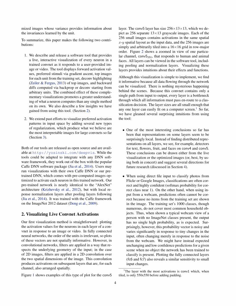
Figure 1. The bottom shows a screenshot from the interactive visualization software. The webcam input is shown, along with the wholelayer of conv5 activations. The selected channel pane shows an enlarged version of the 13x13 conv5151 channel activations. Below it,the deconv starting at the selected channel is shown. On the right, three selections of nine images are shown: synthetic images producedusing the regularized gradient ascent methods described in Section 3, the top 9 image patches from the training set (the images from thetraining set that caused the highest activations for the selected channel), and the deconv of the those top 9 images. All areas highlightedwith a green star relate to the particular selected channel, here conv5151; when the selection changes, these panels update. The topdepicts enlarged numerical optimization results for this and other channels. conv52 is a channel that responds most strongly to dog faces(as evidenced by the top nine images, which are not shown due to space constraints), but it also responds to flowers on the blanket on thebottom and half way up the right side of the image (as seen in the inset red highlight). This response to flowers can be partially seen inthe optimized images but would be missed in an analysis focusing only on the top nine images and their deconv versions, which containno flowers. conv5151 detects different types of faces. The top nine images are all of human faces, but here we see it responds also to thecat’s face (and in Figure 2 a lion’s face). Finally, conv5111 activates strongly for the cat’s face, the optimized images show catlike furand ears, and the top nine images (not shown here) are also all of cats. For this image, the softmax output layer top two predictions are“Egyptian Cat” and “Computer Keyboard.” All figures in this paper are best viewed digitally, in color, significantly zoomed in.

3

mized images whose variance provides information aboutthe invariances learned by the unit.

To summarize, this paper makes the following two contri-butions:

1. We describe and release a software tool that providesa live, interactive visualization of every neuron in atrained convnet as it responds to a user-provided im-age or video. The tool displays forward activation val-ues, preferred stimuli via gradient ascent, top imagesfor each unit from the training set, deconv highlighting(Zeiler & Fergus, 2013) of top images, and backwarddiffs computed via backprop or deconv starting fromarbitrary units. The combined effect of these comple-mentary visualizations promotes a greater understand-ing of what a neuron computes than any single methodon its own. We also describe a few insights we havegained from using this tool. (Section 2).

2. We extend past efforts to visualize preferred activationpatterns in input space by adding several new typesof regularization, which produce what we believe arethe most interpretable images for large convnets so far(Section 3).

Both of our tools are released as open source and are avail-able at http://yosinski.com/deepvis. While thetools could be adapted to integrate with any DNN soft-ware framework, they work out of the box with the popularCaffe DNN software package (Jia et al., 2014). Users mayrun visualizations with their own Caffe DNN or our pre-trained DNN, which comes with pre-computed images op-timized to activate each neuron in this trained network. Ourpre-trained network is nearly identical to the “AlexNet”architecture (Krizhevsky et al., 2012), but with local re-ponse normalization layers after pooling layers following(Jia et al., 2014). It was trained with the Caffe frameworkon the ImageNet 2012 dataset (Deng et al., 2009).

2. Visualizing Live Convnet ActivationsOur first visualization method is straightforward: plottingthe activation values for the neurons in each layer of a con-vnet in response to an image or video. In fully connectedneural networks, the order of the units is irrelevant, so plotsof these vectors are not spatially informative. However, inconvolutional networks, filters are applied in a way that re-spects the underlying geometry of the input; in the caseof 2D images, filters are applied in a 2D convolution overthe two spatial dimensions of the image. This convolutionproduces activations on subsequent layers that are, for eachchannel, also arranged spatially.

Figure 1 shows examples of this type of plot for the conv5

layer. The conv5 layer has size 256×13×13, which we de-pict as 256 separate 13×13 grayscale images. Each of the256 small images contains activations in the same spatialx-y spatial layout as the input data, and the 256 images aresimply and arbitrarily tiled into a 16×16 grid in row-majororder. Figure 2 shows a zoomed in view of one particu-lar channel, conv5151, that responds to human and animalfaces. All layers can be viewed in the software tool, includ-ing pooling and normalization layers. Visualizing theselayers provides intuitions about their effects and functions.

Although this visualization is simple to implement, we findit informative because all data flowing through the networkcan be visualized. There is nothing mysterious happeningbehind the scenes. Because this convnet contains only asingle path from input to output, every layer is a bottleneckthrough which all information must pass en-route to a clas-sification decision. The layer sizes are all small enough thatany one layer can easily fit on a computer screen.1 So far,we have gleaned several surprising intuitions from usingthe tool:

• One of the most interesting conclusions so far hasbeen that representations on some layers seem to besurprisingly local. Instead of finding distributed repre-sentations on all layers, we see, for example, detectorsfor text, flowers, fruit, and faces on conv4 and conv5.These conclusions can be drawn either from the livevisualization or the optimized images (or, best, by us-ing both in concert) and suggest several directions forfuture research (discussed in Section 4).

• When using direct file input to classify photos fromFlickr or Google Images, classifications are often cor-rect and highly confident (softmax probability for cor-rect class near 1). On the other hand, when using in-put from a webcam, predictions often cannot be cor-rect because no items from the training set are shownin the image. The training set’s 1000 classes, thoughnumerous, do not cover most common household ob-jects. Thus, when shown a typical webcam view of aperson with no ImageNet classes present, the outputhas no single high probability, as is expected. Sur-prisingly, however, this probability vector is noisy andvaries significantly in response to tiny changes in theinput, often changing merely in response to the noisefrom the webcam. We might have instead expectedunchanging and low confidence predictions for a givenscene when no object the network has been trained toclassify is present. Plotting the fully connected layers(fc6 and fc7) also reveals a similar sensitivity to smallinput changes.

1The layer with the most activations is conv1 which, whentiled, is only 550x550 before adding padding.

4

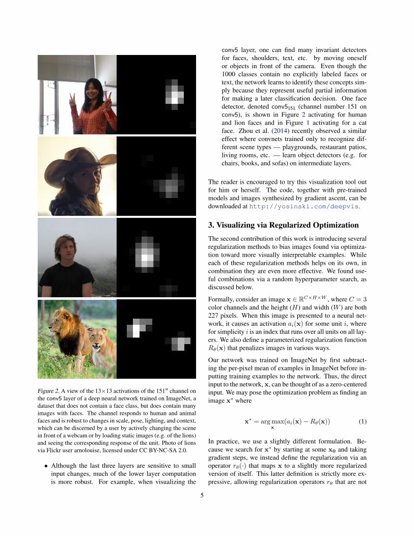
Figure 2. A view of the 13×13 activations of the 151st channel onthe conv5 layer of a deep neural network trained on ImageNet, adataset that does not contain a face class, but does contain manyimages with faces. The channel responds to human and animalfaces and is robust to changes in scale, pose, lighting, and context,which can be discerned by a user by actively changing the scenein front of a webcam or by loading static images (e.g. of the lions)and seeing the corresponding response of the unit. Photo of lionsvia Flickr user arnolouise, licensed under CC BY-NC-SA 2.0.

• Although the last three layers are sensitive to smallinput changes, much of the lower layer computationis more robust. For example, when visualizing the

conv5 layer, one can find many invariant detectorsfor faces, shoulders, text, etc. by moving oneselfor objects in front of the camera. Even though the1000 classes contain no explicitly labeled faces ortext, the network learns to identify these concepts sim-ply because they represent useful partial informationfor making a later classification decision. One facedetector, denoted conv5151 (channel number 151 onconv5), is shown in Figure 2 activating for humanand lion faces and in Figure 1 activating for a catface. Zhou et al. (2014) recently observed a similareffect where convnets trained only to recognize dif-ferent scene types — playgrounds, restaurant patios,living rooms, etc. — learn object detectors (e.g. forchairs, books, and sofas) on intermediate layers.

The reader is encouraged to try this visualization tool outfor him or herself. The code, together with pre-trainedmodels and images synthesized by gradient ascent, can bedownloaded at http://yosinski.com/deepvis.

3. Visualizing via Regularized OptimizationThe second contribution of this work is introducing severalregularization methods to bias images found via optimiza-tion toward more visually interpretable examples. Whileeach of these regularization methods helps on its own, incombination they are even more effective. We found use-ful combinations via a random hyperparameter search, asdiscussed below.

Formally, consider an image x ∈ RC×H×W , where C = 3color channels and the height (H) and width (W ) are both227 pixels. When this image is presented to a neural net-work, it causes an activation ai(x) for some unit i, wherefor simplicity i is an index that runs over all units on all lay-ers. We also define a parameterized regularization functionRθ(x) that penalizes images in various ways.

Our network was trained on ImageNet by first subtract-ing the per-pixel mean of examples in ImageNet before in-putting training examples to the network. Thus, the directinput to the network, x, can be thought of as a zero-centeredinput. We may pose the optimization problem as finding animage x∗ where

x∗ = argmaxx

(ai(x)−Rθ(x)) (1)

In practice, we use a slightly different formulation. Be-cause we search for x∗ by starting at some x0 and takinggradient steps, we instead define the regularization via anoperator rθ(·) that maps x to a slightly more regularizedversion of itself. This latter definition is strictly more ex-pressive, allowing regularization operators rθ that are not

5

the gradient of any Rθ. This method is easy to implementwithin a gradient descent framework by simply alternatingbetween taking a step toward the gradient of ai(x) and tak-ing a step in the direction given by rθ. With a gradientdescent step size of η, a single step in this process appliesthe update:

x← rθ

(x+ η

∂ai∂x

)(2)

We investigated the following four regularizations. All aredesigned to overcome different pathologies commonly en-countered by gradient descent without regularization.

L2 decay: A common regularization, L2 decay penalizeslarge values and is implemented as rθ(x) = (1−θdecay)·x.L2 decay tends to prevent a small number of extreme pixelvalues from dominating the example image. Such extremesingle-pixel values neither occur naturally with great fre-quency nor are useful for visualization. L2 decay was alsoused by Simonyan et al. (2013).

Gaussian blur: Producing images via gradient ascenttends to produce examples with high frequency informa-tion (see Supplementary Section S1 for a possible reason).While these images cause high activations, they are neitherrealistic nor interpretable (Nguyen et al., 2014). A usefulregularization is thus to penalize high frequency informa-tion. We implement this as a Gaussian blur step rθ(x) =GaussianBlur(x, θb width). Convolving with a blur ker-nel is more computationally expensive than the other reg-ularization methods, so we added another hyperparameterθb every to allow, for example, blurring every several op-timization steps instead of every step. Blurring an imagemultiple times with a small width Gaussian kernel is equiv-alent to blurring once with a larger width kernel, and theeffect will be similar even if the image changes slightlyduring the optimization process. This technique thus low-ers computational costs without limiting the expressivenessof the regularization. Mahendran & Vedaldi (2014) used apenalty with a similar effect to blurring, called total varia-tion, in their work reconstructing images from layer codes.

Clipping pixels with small norm: The first two regulariza-tions suppress high amplitude and high frequency informa-tion, so after applying both, we are left with an x∗ that con-tains somewhat small, somewhat smooth values. However,x∗ will still tend to contain non-zero pixel values every-where. Even if some pixels in x∗ show the primary objector type of input causing the unit under consideration to ac-tivate, the gradient with respect to all other pixels in x∗ willstill generally be non-zero, so these pixels will also shift toshow some pattern as well, contributing in whatever smallway they can to ultimately raise the chosen unit’s activa-tion. We wish to bias the search away from such behavior

and instead show only the main object, letting other regionsbe exactly zero if they are not needed. We implement thisbias using an rθ(x) that computes the norm of each pixel(over red, green, and blue channels) and then sets any pix-els with small norm to zero. The threshold for the norm,θn pct, is specified as a percentile of all pixel norms in x.

Clipping pixels with small contribution: Instead of clip-ping pixels with small norms, we can try something slightlysmarter and clip pixels with small contributions to the acti-vation. One way of computing a pixel’s contribution to anactivation is to measure how much the activation increasesor decreases when the pixel is set to zero; that is, to com-pute the contribution as |ai(x)− ai(x−j)|, where x−j is xbut with the jth pixel set to zero. This approach is straight-forward but prohibitively slow, requiring a forward passfor every pixel. Instead, we approximate this process bylinearizing ai(x) around x, in which case the contributionof each dimension of x can be estimated as the elemen-twise product of x and the gradient. We then sum overall three channels and take the absolute value, computing|∑c x ◦ ∇xai(x)|. We use the absolute value to find pix-

els with small contribution in either direction, positive ornegative. While we could choose to keep the pixel transi-tions where setting the pixel to zero would result in a largeactivation increase, these shifts are already handled by gra-dient ascent, and here we prefer to clip only the pixels thatare deemed not to matter, not to take large gradient stepsoutside the region where the linear approximation is mostvalid. We define this rθ(x) as the operation that sets pixelswith contribution under the θc pct percentile to zero.

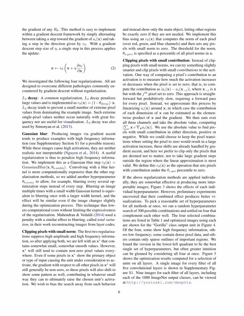
If the above regularization methods are applied individu-ally, they are somewhat effective at producing more inter-pretable images; Figure 3 shows the effects of each indi-vidual hyperparameter. However, preliminary experimentsuncovered that their combined effect produces better vi-sualizations. To pick a reasonable set of hyperparametersfor all methods at once, we ran a random hyperparametersearch of 300 possible combinations and settled on four thatcomplement each other well. The four selected combina-tions are listed in Table 1 and optimized images using eachare shown for the “Gorilla” class output unit in Figure 4.Of the four, some show high frequency information, oth-ers low frequency; some contain dense pixel data, and oth-ers contain only sparse outlines of important regions. Wefound the version in the lower-left quadrant to be the bestsingle set of hyperparameters, but often greater intuitioncan be gleaned by considering all four at once. Figure 5shows the optimization results computed for a selection ofunits on all layers. A single image for every filter of allfive convolutional layers is shown in Supplementary Fig-ure S1. Nine images for each filter of all layers, includingeach of the 1000 ImageNet output classes, can be viewedat http://yosinski.com/deepvis.

6

Figure 4. Visualizations of the preferred inputs for different class units on layer fc8, the 1000-dimensional output of the network justbefore the final softmax. In the lower left are 9 visualizations each (in 3×3 grids) for four different sets of regularization hyperparametersfor the Gorilla class (Table 1). For all other classes, we have selected four interpretable visualizations produced by our regularizedoptimization method. We chose the four combinations of regularization hyperparameters by performing a random hyperparameter searchand selecting combinations that complement each other. For example, the lower left quadrant tends to show lower frequency patterns,the upper right shows high frequency patterns, and the upper left shows a sparse set of important regions. Often greater intuition canbe gleaned by considering all four at once. In nearly every case, we have found that one can guess what class a neuron represents byviewing sets of these optimized, preferred images. Best viewed electronically, zoomed in.7

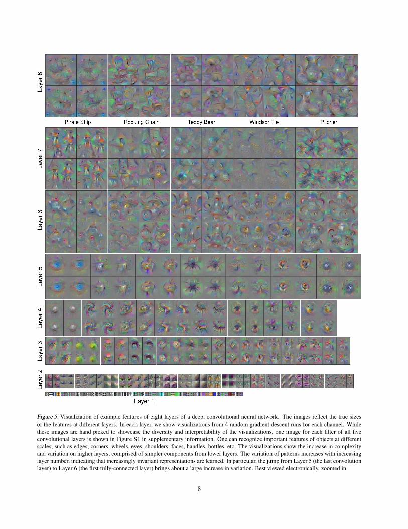
Figure 5. Visualization of example features of eight layers of a deep, convolutional neural network. The images reflect the true sizesof the features at different layers. In each layer, we show visualizations from 4 random gradient descent runs for each channel. Whilethese images are hand picked to showcase the diversity and interpretability of the visualizations, one image for each filter of all fiveconvolutional layers is shown in Figure S1 in supplementary information. One can recognize important features of objects at differentscales, such as edges, corners, wheels, eyes, shoulders, faces, handles, bottles, etc. The visualizations show the increase in complexityand variation on higher layers, comprised of simpler components from lower layers. The variation of patterns increases with increasinglayer number, indicating that increasingly invariant representations are learned. In particular, the jump from Layer 5 (the last convolutionlayer) to Layer 6 (the first fully-connected layer) brings about a large increase in variation. Best viewed electronically, zoomed in.

8

✓ dec

ay=

0.5

✓ npct=

95✓ c

pct=

95✓ b

width

=1.0

✓ bev

ery=

4

✓ dec

ay=

0.0

✓ npct=

0✓ c

pct=

0✓ b

every=

10✓ b

width

=0.0

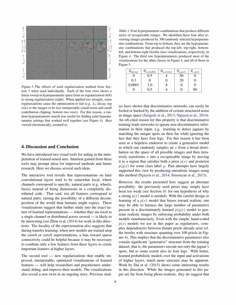
Figure 3. The effects of each regularization method from Sec-tion 3 when used individually. Each of the four rows shows alinear sweep in hyperparameter space from no regularization (left)to strong regularization (right). When applied too strongly, someregularizations cause the optimization to fail (e.g. L2 decay, toprow) or the images to be less interpretable (small norm and smallcontribution clipping, bottom two rows). For this reason, a ran-dom hyperparameter search was useful for finding joint hyperpa-rameter settings that worked well together (see Figure 4). Bestviewed electronically, zoomed in.

4. Discussion and ConclusionWe have introduced two visual tools for aiding in the inter-pretation of trained neural nets. Intuition gained from thesetools may prompt ideas for improved methods and futureresearch. Here we discuss several such ideas.

The interactive tool reveals that representations on laterconvolutional layers tend to be somewhat local, wherechannels correspond to specific, natural parts (e.g. wheels,faces) instead of being dimensions in a completely dis-tributed code. That said, not all features correspond tonatural parts, raising the possibility of a different decom-position of the world than humans might expect. Thesevisualizations suggest that further study into the exact na-ture of learned representations — whether they are local toa single channel or distributed across several — is likely tobe interesting (see Zhou et al. (2014) for work in this direc-tion). The locality of the representation also suggests thatduring transfer learning, when new models are trained atopthe conv4 or conv5 representations, a bias toward sparseconnectivity could be helpful because it may be necessaryto combine only a few features from these layers to createimportant features at higher layers.

The second tool — new regularizations that enable im-proved, interpretable, optimized visualizations of learnedfeatures — will help researchers and practitioners under-stand, debug, and improve their models. The visualizationsalso reveal a new twist in an ongoing story. Previous stud-

Table 1. Four hyperparameter combinations that produce differentstyles of recognizable images. We identified these four after re-viewing images produced by 300 randomly selected hyperparam-eter combinations. From top to bottom, they are the hyperparam-eter combinations that produced the top-left, top-right, bottom-left, and bottom-right Gorilla class visualizations, respectively, inFigure 4. The third row hyperparameters produced most of thevisualizations for the other classes in Figure 4, and all of those inFigure 5.

θdecay θb width θb every θn pct θc pct

0 0.5 4 50 00.3 0 0 20 0

0.0001 1.0 4 0 00 0.5 4 0 90

ies have shown that discriminative networks can easily befooled or hacked by the addition of certain structured noisein image space (Szegedy et al., 2013; Nguyen et al., 2014).An oft-cited reason for this property is that discriminativetraining leads networks to ignore non-discriminative infor-mation in their input, e.g. learning to detect jaguars bymatching the unique spots on their fur while ignoring thefact that they have four legs. For this reason it has beenseen as a hopeless endeavor to create a generative modelin which one randomly samples an x from a broad distri-bution on the space of all possible images and then itera-tively transforms x into a recognizable image by movingit to a region that satisfies both a prior p(x) and posteriorp(y|x) for some class label y. Past attempts have largelysupported this view by producing unrealistic images usingthis method (Nguyen et al., 2014; Simonyan et al., 2013).

However, the results presented here suggest an alternatepossibility: the previously used priors may simply havebeen too weak (see Section S1 for one hypothesis of whya strong p(x) model is needed). With the careful design orlearning of a p(x) model that biases toward realism, onemay be able to harness the large number of parameterspresent in a discriminately learned p(y|x) model to gen-erate realistic images by enforcing probability under bothmodels simultaneously. Even with the simple, hand-codedp(x) models we use in this paper as regularizers, com-plex dependencies between distant pixels already arise (cf.the beetles with structure spanning over 100 pixels in Fig-ure 4). This implies that the discriminative parameters alsocontain significant “generative” structure from the trainingdataset; that is, the parameters encode not only the jaguar’sspots, but to some extent also its four legs. With better,learned probabilistic models over the input and activationsof higher layers, much more structure may be apparent.Work by Dai et al. (2015) shows some interesting resultsin this direction. While the images generated in this pa-per are far from being photo-realistic, they do suggest that

9

transferring discriminatively trained parameters to gener-ative models — opposite the direction of the usual unsu-pervised pretraining approach — may be a fruitful area forfurther investigation.

AcknowledgmentsThe authors would like to thank the NASA Space Technol-ogy Research Fellowship (JY) for funding, Wendy Shang,Yoshua Bengio, Brian Cheung, and Andrej Karpathy forhelpful discussions, and Freckles the cat for her felinecountenance.

ReferencesBergstra, James, Breuleux, Olivier, Bastien, Frederic, Lam-

blin, Pascal, Pascanu, Razvan, Desjardins, Guillaume, Turian,Joseph, Warde-Farley, David, and Bengio, Yoshua. Theano: aCPU and GPU math expression compiler. In Proceedings ofthe Python for Scientific Computing Conference (SciPy), June2010. Oral Presentation.

Collobert, Ronan, Kavukcuoglu, Koray, and Farabet, Clement.Torch7: A matlab-like environment for machine learning.In BigLearn, NIPS Workshop, number EPFL-CONF-192376,2011.

Dai, Jifeng, Lu, Yang, and Wu, Ying Nian. Generative modelingof convolutional neural networks. In International Conferenceon Learning Representations (ICLR), 2015.

Deng, Jia, Dong, Wei, Socher, Richard, Li, Li-Jia, Li, Kai,and Fei-Fei, Li. Imagenet: A large-scale hierarchical imagedatabase. In Computer Vision and Pattern Recognition, 2009.CVPR 2009. IEEE Conference on, pp. 248–255. IEEE, 2009.

Erhan, Dumitru, Bengio, Yoshua, Courville, Aaron, and Vin-cent, Pascal. Visualizing higher-layer features of a deep net-work. Technical report, Technical report, University of Mon-treal, 2009.

Glorot, Xavier, Bordes, Antoine, and Bengio, Yoshua. Deepsparse rectifier networks. In Proceedings of the 14th Inter-national Conference on Artificial Intelligence and Statistics.JMLR W&CP Volume, volume 15, pp. 315–323, 2011.

Goodfellow, Ian J, Warde-Farley, David, Lamblin, Pascal, Du-moulin, Vincent, Mirza, Mehdi, Pascanu, Razvan, Bergstra,James, Bastien, Frederic, and Bengio, Yoshua. Pylearn2:a machine learning research library. arXiv preprintarXiv:1308.4214, 2013.

Goodfellow, Ian J, Shlens, Jonathon, and Szegedy, Christian. Ex-plaining and Harnessing Adversarial Examples. ArXiv e-prints,December 2014.

Hannun, A., Case, C., Casper, J., Catanzaro, B., Diamos, G.,Elsen, E., Prenger, R., Satheesh, S., Sengupta, S., Coates, A.,and Ng, A. Y. Deep Speech: Scaling up end-to-end speechrecognition. ArXiv e-prints, December 2014.

Hinton, Geoffrey E, Srivastava, Nitish, Krizhevsky, Alex,Sutskever, Ilya, and Salakhutdinov, Ruslan R. Improving neu-ral networks by preventing co-adaptation of feature detectors.arXiv preprint arXiv:1207.0580, 2012.

Jia, Yangqing, Shelhamer, Evan, Donahue, Jeff, Karayev, Sergey,Long, Jonathan, Girshick, Ross, Guadarrama, Sergio, and Dar-rell, Trevor. Caffe: Convolutional architecture for fast featureembedding. arXiv preprint arXiv:1408.5093, 2014.

Krizhevsky, Alex, Sutskever, Ilya, and Hinton, Geoff. Imagenetclassification with deep convolutional neural networks. InAdvances in Neural Information Processing Systems 25, pp.1106–1114, 2012.

Lin, Tsung-Yi, Maire, Michael, Belongie, Serge, Hays, James,Perona, Pietro, Ramanan, Deva, Dollar, Piotr, and Zitnick,C. Lawrence. Microsoft COCO: common objects in context.CoRR, abs/1405.0312, 2014. URL http://arxiv.org/abs/1405.0312.

Mahendran, A. and Vedaldi, A. Understanding Deep Image Rep-resentations by Inverting Them. ArXiv e-prints, November2014.

Nguyen, Anh, Yosinski, Jason, and Clune, Jeff. Deep Neural Net-works are Easily Fooled: High Confidence Predictions for Un-recognizable Images. ArXiv e-prints, December 2014.

Schroff, F., Kalenichenko, D., and Philbin, J. FaceNet: A Uni-fied Embedding for Face Recognition and Clustering. ArXive-prints, March 2015.

Simonyan, Karen, Vedaldi, Andrea, and Zisserman, Andrew.Deep inside convolutional networks: Visualising imageclassification models and saliency maps. arXiv preprintarXiv:1312.6034, presented at ICLR Workshop 2014, 2013.

Szegedy, Christian, Zaremba, Wojciech, Sutskever, Ilya, Bruna,Joan, Erhan, Dumitru, Goodfellow, Ian J., and Fergus, Rob. In-triguing properties of neural networks. CoRR, abs/1312.6199,2013.

Taigman, Yaniv, Yang, Ming, Ranzato, Marc’Aurelio, and Wolf,Lior. Deepface: Closing the gap to human-level performancein face verification. In Computer Vision and Pattern Recogni-tion (CVPR), 2014 IEEE Conference on, pp. 1701–1708. IEEE,2014.

Torralba, Antonio and Oliva, Aude. Statistics of natural imagecategories. Network: computation in neural systems, 14(3):391–412, 2003.

Yosinski, J., Clune, J., Bengio, Y., and Lipson, H. How trans-ferable are features in deep neural networks? In Ghahramani,Z., Welling, M., Cortes, C., Lawrence, N.D., and Weinberger,K.Q. (eds.), Advances in Neural Information Processing Sys-tems 27, pp. 3320–3328. Curran Associates, Inc., December2014.

Zeiler, Matthew D and Fergus, Rob. Visualizing and un-derstanding convolutional neural networks. arXiv preprintarXiv:1311.2901, 2013.

Zhou, Bolei, Khosla, Aditya, Lapedriza, Agata, Oliva, Aude, andTorralba, Antonio. Object detectors emerge in deep scene cnns.CoRR, abs/1412.6856, 2014. URL http://arxiv.org/abs/1412.6856.

10

Supplementary Information for:Understanding Neural Networks Through Deep Visualization

Jason Yosinski YOSINSKI@CS.CORNELL.EDUJeff Clune JEFFCLUNE@UWYO.EDUAnh Nguyen ANGUYEN8@UWYO.EDUThomas Fuchs FUCHS@CALTECH.EDUHod Lipson HOD.LIPSON@CORNELL.EDU

S1. Why are gradient optimized imagesdominated by high frequencies?

In the main text we mentioned that images produced bygradient ascent to maximize the activations of neurons inconvolutional networks tend to be dominated by high fre-quency information (cf. the left column of Figure 3). Onehypothesis for why this occurs centers around the differingstatistics of the activations of channels in a convnet. Theconv1 layer consists of blobs of color and oriented Gaboredge filters of varying frequencies. The average activationvalues (after the rectifier) of the edge filters vary acrossfilters, with low frequency filters generally having muchhigher average activation values than high frequency filters.In one experiment we observed that the average activationvalues of the five lowest frequency edge filters was 90 ver-sus an average for the five highest frequency filters of 5.4, adifference of a factor of 17 (manuscript in preparation)2,3.The activation values for blobs of color generally fall in themiddle of the range. This phenomenon likely arises for rea-sons related to the 1/f power spectrum of natural images inwhich low spatial frequencies tend to contain higher energythan high spatial frequencies (Torralba & Oliva, 2003).

Now consider the connections from the conv1 filters to asingle unit on conv2. In order to merge information fromboth low frequency and high frequency conv1 filters, theconnection weights from high frequency conv1 units maygenerally have to be larger than connections from low fre-quency conv1 units in order to allow both signals to affectthe conv2 unit’s activation similarly. If this is the case, thendue to the larger multipliers, the activation of this particularconv2 unit is affected more by small changes in the activa-tions of high frequency filters than low frequency filters.

2Li, Yosinski, Clune, Song, Hopcroft, Lipson. 2015. Howsimilar are features learned by different deep neural networks? Inpreparation.

3Activation values are averaged over the ImageNet validationset, over all spatial positions, over the channels with the five{highest, lowest} frequencies, and over four separately trainednetworks.

Seen in the other direction: when gradient information ispassed from higher layers to lower layers during backprop,the partial derivative arriving at this conv2 unit (a scalar)will be passed backward and multiplied by larger valueswhen destined for high frequency conv1 filters than low fre-quency filters. Thus, following the gradient in pixel spacemay tend to produce an overabundance of high frequencychanges instead of low frequency changes.

The above discussion focuses on the differing statistics ofedge filters in conv1, but note that activation statistics onsubsequent layers also vary across each layer.4 This mayproduce a similar (though more subtle to observe) effect inwhich rare higher layer features are also overrepresentedcompared to more common higher layer features.

Of course, this hypothesis is only one tentative explanationfor why high frequency information dominates the gradi-ent. It relies on the assumption that the average activationof a unit is a representative statistic of the whole distribu-tion of activations for that unit. In our observation thishas been the case, with most units having similar, albeitscaled, distributions. However, more study is needed be-fore a definitive conclusion can be reached.

S2. Conv Layer MontagesOne example optimized image using the hyperparametersettings from the third row of Table 1 for every filter of allfive convolutional layers is shown in Figure S1.

4We have observed that statistics vary on higher layers, but ina different manner: most channels on these layers have similar av-erage activations, with most of the variance across channels beingdominated by a small number of channels with unusually smallor unusually large averages (Li, Yosinski, Clune, Song, Hopcroft,Lipson. 2015. How similar are features learned by different deepneural networks? In preparation.)

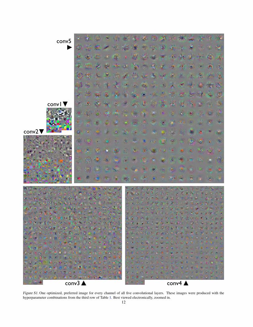
conv5

conv3 conv4

conv2

conv1

Figure S1. One optimized, preferred image for every channel of all five convolutional layers. These images were produced with thehyperparameter combinations from the third row of Table 1. Best viewed electronically, zoomed in.

12