Understanding network dynamics of a bike-sharing system to

Understanding network dynamics of a bike-sharingsystem to enhance inventory self-balancing∗

CS5834 Intro to Urban Computing - Project†

Alexander RodriguezDepartment of Computer Science

Virginia Tech

Anika TabassumDepartment of Computer Science

Virginia Tech

Bumsik KimDeparment of Civil and

Environmental EngineeringVirginia Tech

ABSTRACTHow does the network dynamics from a bike-share systemprovide insights to enhance its inventory self-balance? In thiswork, we model station demand and route flow across timeand weather considerations. These models are used to makelong term and real-time decisions about incentives for riders.Such incentives aim to improve inventory self-balancing,which increments service satisfaction and company’s profit.Therefore, we propose using a visualization to support deci-sion making related to these incentives across different timesof the day.

KEYWORDSBike-sharing system, urban computing, dynamics visualiza-tion

ACM Reference Format:Alexander Rodriguez, Anika Tabassum, and Bumsik Kim. 2018.Understanding network dynamics of a bike-sharing system to en-hance inventory self-balancing: CS5834 Intro to Urban Computing- Project. In Proceedings of ACM Conference (Conference’17). ACM,New York, NY, USA, Article 4, 12 pages. https://doi.org/10.1145/nnnnnnn.nnnnnnn

1 INTRODUCTIONSince the bike-sharing system launched in the U.S., the sys-tem has grown dramatically. According to the National As-sociation of City Transportation Officials (NACTO), in 2010,

∗Produces the permission block, and copyright information†The full version of the author’s guide is available as acmart.pdf document

Permission to make digital or hard copies of part or all of this work forpersonal or classroom use is granted without fee provided that copies arenot made or distributed for profit or commercial advantage and that copiesbear this notice and the full citation on the first page. Copyrights for third-party components of this work must be honored. For all other uses, contactthe owner/author(s).Conference’17, July 2017, Washington, DC, USA© 2018 Copyright held by the owner/author(s).ACM ISBN 978-x-xxxx-xxxx-x/YY/MM.https://doi.org/10.1145/nnnnnnn.nnnnnnn

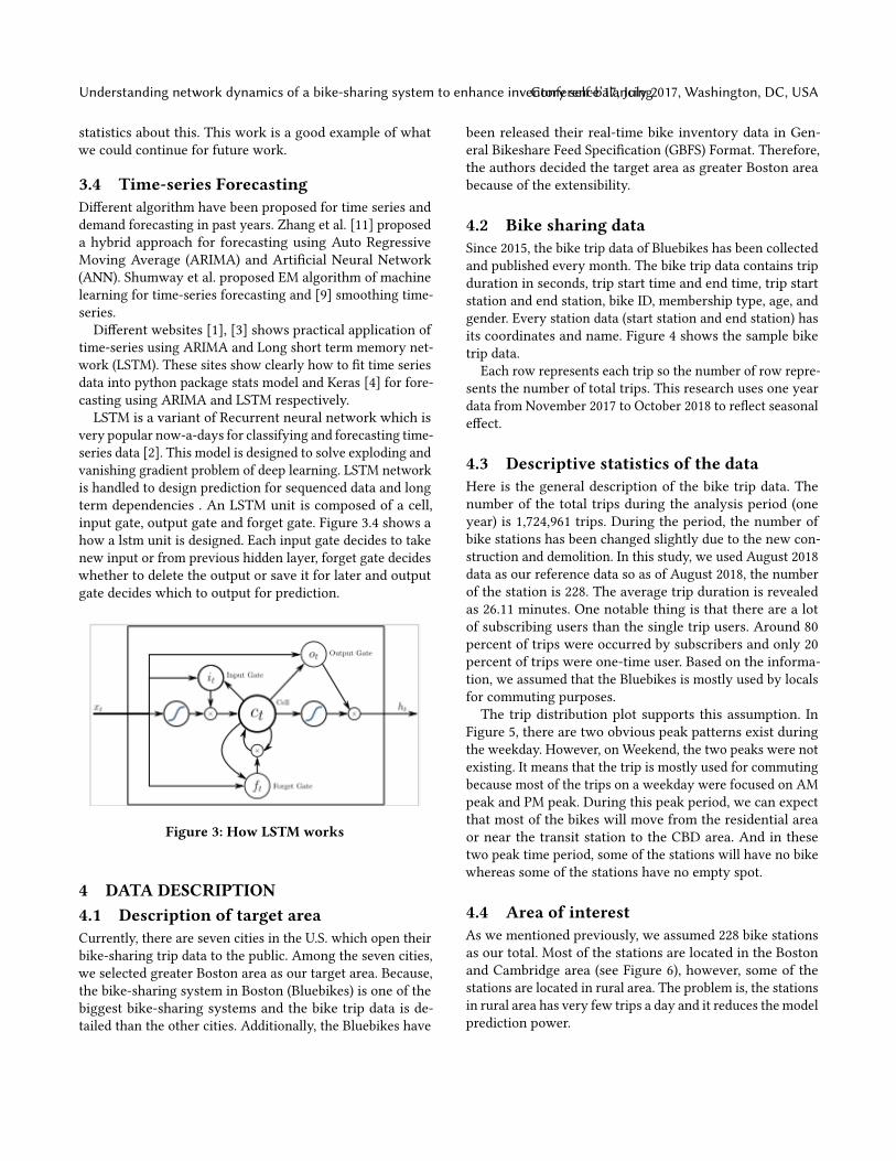
the total number of bike-sharing trip was 320,000, however,in 2017, the number of bike-sharing trip was 35 millions.

Figure 1: Annual growth ofBike share ridership inU.S.

Especially, the number of bikes in 2016 was 42,500 whilethe number of bikes in 2017 was 100,000 due to the introduc-ing ’dockless’ bike sharing system. The dockless system doesnot require a conventional parking spot, instead, they usedsmartphone applications to inform the location of availablebikes. In other words, the users in the dockless system canpark a bike wherever they want. However, still the system isin an initial stage and most of the cities have adopted tradi-tional bike-sharing systems with bike stations. The docklessbike-sharing system also has pros and cons, however, thisstudy will focus on the traditional station-based bike-sharingsystem.

Every bike-sharing stations have different demand by timeof the day. Sometimes, some of the stations are full of thebike so the users cannot park a bike. On the other hand,during the peak hour, some of the stations have no availablebike. To keep it balanced, the operator uses force-balancingwhich means bike moving truck.

The balancing is important for efficient usage of the assetof a station. In the short term, the imbalanced bike inventorytakes chances of using a bike to potential users. At the veryworst, In the long term, the users give up their expectationto the bike sharing system and no one wants to use thebike-sharing system. In this study, we defined self-balancingas a trip by user and force-balancing as a trip by operatorstruck. And we assume self-balancing is the ideal case becauseself-balancing requires no additional cost.

https://doi.org/10.1145/nnnnnnn.nnnnnnn



Conference’17, July 2017, Washington, DC, USA Alexander Rodriguez, Anika Tabassum, and Bumsik Kim

One policy alternative to improve self-balancing is byincentivizing routing from low demand stations to high de-mand stations. For instance, in Figure 2, we can note thattrips from D to A could be incentivized by splitting in incen-tives from D to B and B to A. This routing technique wouldbe helpful when there are not many people going from D toA.

Figure 2: An example of self-balancing incentive

The self-balancing and incentive could reduce the man-agement of system operator as well as enhance the reliabilityof bike sharing system itself. If the bike-sharing system runsby self-balancing, the operator does not need to dispatchforce-balance vehicle and the operator could save cost. Next,the users start to think the bike-sharing system is reliableif they can borrow a bike when they want. Finally, the self-balancing could change people’s behavior and could increasebike mode share.

2 PROBLEM DEFINITION2.1 Problem statementAs noted before, imbalanced bike inventory disturbs a poten-tial user from using the system. Currently, bike-sharing sys-tems require force-balanced interventions which are costlyand do not fully satisfy demand. The trip data from bike-sharing system shows potential to bring insights to takeaction, as for example, give incentives to users of specificroutes, so that they transport bikes to where the users needthem to be.

2.2 Expected benefitsFirst of all, we can expect that self-balancing could reduce theoperational cost of bike-sharing system. From the literature,the bike distribution cost is one of the major operational cost.However, more self-balance might reduces the moving truckand therefore, the operator could save the cost. Next, theusers can trust the bike-sharing system if they can hire a bikewhenever, wherever they want. In long term view, the moreself-balancing increases bike share and reduces congestion.

3 RELATEDWORK3.1 Balancing Bike-sharing SystemsMany researchers have been tried to solve balance problem.[8] pointed out that the major operational cost is rebalanc-ing cost. To reduct the cost, they tried to use two methods:determining service level requirements at each bike shar-ing station, and designing near optimal vehicle routes torebalance the inventory. In this study, they utilized Markov-chain and clustering to suggest proper routes. [5] introducesthe dynamic public bike-sharing balancing problem to at-tenuate that there is more demand in certain stations thanothers. This problem routes bikes to balance the network.Its main contribution is a mathematical formulation for theoptimization. While we share a similar goal with this work,we opt not to do a optimization and instead we want to usea visualization. One last study, [10], suggests incentives tothe user who have willing to repositioning bike by usingcrowd-sourcing mechanism and surveys. The paper revealedthat the self-balancing works with dynamic incentive wereaccepted 60 percents of participants.

3.2 Machine Learning in Bike-sharingSystems

In literature, there have been some applications of machinelearning in bike-sharing systems. For example, [7] workedto estimate the traffic in a bike-sharing system by includ-ing demand prediction and trip duration with regressionmodels that consider meteorological conditions and impor-tant events in the city. In our work, we partially adopt thisidea and include meteorological conditions as we think theyshould be highly predictive for demand forecasting.

[12] worked in a similar problem to ours in a bike-sharingsystem where they wanted to predict the trip destination andduration. For the trip destination inference they used MART(Multiple Additive Regression Trees) and the estimation ofthe trip duration they used Lasso. To build these modelsthey used features from the user (gender, age), the departuretime, and the bike stations location. In contrast to them, wedonâĂŹt have personal information about users. In addition,this paper suggests using Manhattan distance in estimatingtravel distances in a city.

3.3 Visualization of Urban Dynamics[6] created a visualization tool for taxi trips in a city calledTaxiViz. In their case study, they examine how trip frequencyvary for each day of the week for each neighborhood. Theirwork recognizes the importance of considering transporta-tion hubs to understand the flow of taxis around the city, asfor example, airports and major train stations. In addition, itexploits relationships among origin-destination and displays

Understanding network dynamics of a bike-sharing system to enhance inventory self-balancingConference’17, July 2017, Washington, DC, USA

statistics about this. This work is a good example of whatwe could continue for future work.

3.4 Time-series ForecastingDifferent algorithm have been proposed for time series anddemand forecasting in past years. Zhang et al. [11] proposeda hybrid approach for forecasting using Auto RegressiveMoving Average (ARIMA) and Artificial Neural Network(ANN). Shumway et al. proposed EM algorithm of machinelearning for time-series forecasting and [9] smoothing time-series.Different websites [1], [3] shows practical application of

time-series using ARIMA and Long short term memory net-work (LSTM). These sites show clearly how to fit time seriesdata into python package stats model and Keras [4] for fore-casting using ARIMA and LSTM respectively.LSTM is a variant of Recurrent neural network which is

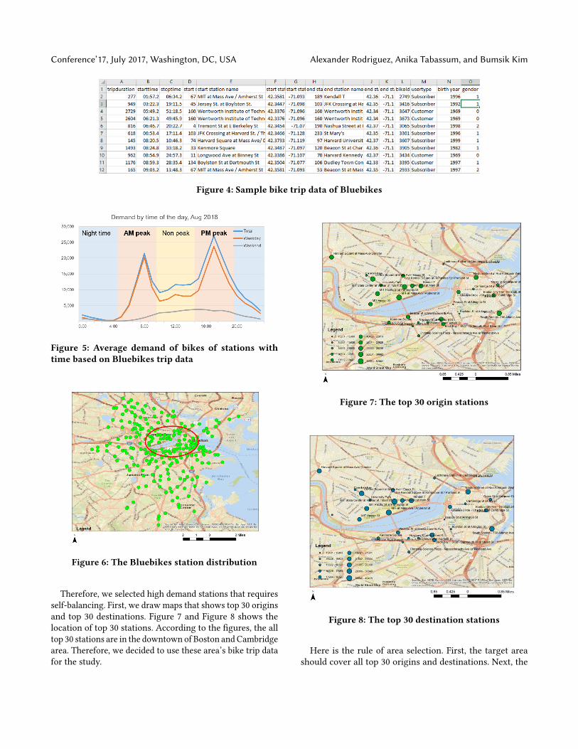
very popular now-a-days for classifying and forecasting time-series data [2]. This model is designed to solve exploding andvanishing gradient problem of deep learning. LSTM networkis handled to design prediction for sequenced data and longterm dependencies . An LSTM unit is composed of a cell,input gate, output gate and forget gate. Figure 3.4 shows ahow a lstm unit is designed. Each input gate decides to takenew input or from previous hidden layer, forget gate decideswhether to delete the output or save it for later and outputgate decides which to output for prediction.

Figure 3: How LSTM works

4 DATA DESCRIPTION4.1 Description of target areaCurrently, there are seven cities in the U.S. which open theirbike-sharing trip data to the public. Among the seven cities,we selected greater Boston area as our target area. Because,the bike-sharing system in Boston (Bluebikes) is one of thebiggest bike-sharing systems and the bike trip data is de-tailed than the other cities. Additionally, the Bluebikes have

been released their real-time bike inventory data in Gen-eral Bikeshare Feed Specification (GBFS) Format. Therefore,the authors decided the target area as greater Boston areabecause of the extensibility.

4.2 Bike sharing dataSince 2015, the bike trip data of Bluebikes has been collectedand published every month. The bike trip data contains tripduration in seconds, trip start time and end time, trip startstation and end station, bike ID, membership type, age, andgender. Every station data (start station and end station) hasits coordinates and name. Figure 4 shows the sample biketrip data.

Each row represents each trip so the number of row repre-sents the number of total trips. This research uses one yeardata from November 2017 to October 2018 to reflect seasonaleffect.

4.3 Descriptive statistics of the dataHere is the general description of the bike trip data. Thenumber of the total trips during the analysis period (oneyear) is 1,724,961 trips. During the period, the number ofbike stations has been changed slightly due to the new con-struction and demolition. In this study, we used August 2018data as our reference data so as of August 2018, the numberof the station is 228. The average trip duration is revealedas 26.11 minutes. One notable thing is that there are a lotof subscribing users than the single trip users. Around 80percent of trips were occurred by subscribers and only 20percent of trips were one-time user. Based on the informa-tion, we assumed that the Bluebikes is mostly used by localsfor commuting purposes.The trip distribution plot supports this assumption. In

Figure 5, there are two obvious peak patterns exist duringthe weekday. However, on Weekend, the two peaks were notexisting. It means that the trip is mostly used for commutingbecause most of the trips on a weekday were focused on AMpeak and PM peak. During this peak period, we can expectthat most of the bikes will move from the residential areaor near the transit station to the CBD area. And in thesetwo peak time period, some of the stations will have no bikewhereas some of the stations have no empty spot.

4.4 Area of interestAs we mentioned previously, we assumed 228 bike stationsas our total. Most of the stations are located in the Bostonand Cambridge area (see Figure 6), however, some of thestations are located in rural area. The problem is, the stationsin rural area has very few trips a day and it reduces the modelprediction power.


Figure 4: Sample bike trip data of Bluebikes

Figure 5: Average demand of bikes of stations withtime based on Bluebikes trip data

Figure 6: The Bluebikes station distribution

Therefore, we selected high demand stations that requiresself-balancing. First, we draw maps that shows top 30 originsand top 30 destinations. Figure 7 and Figure 8 shows thelocation of top 30 stations. According to the figures, the alltop 30 stations are in the downtown of Boston and Cambridgearea. Therefore, we decided to use these area’s bike trip datafor the study.

Figure 7: The top 30 origin stations

Figure 8: The top 30 destination stations

Here is the rule of area selection. First, the target areashould cover all top 30 origins and destinations. Next, the


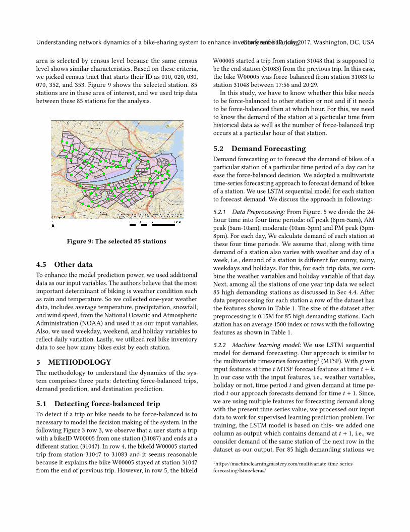
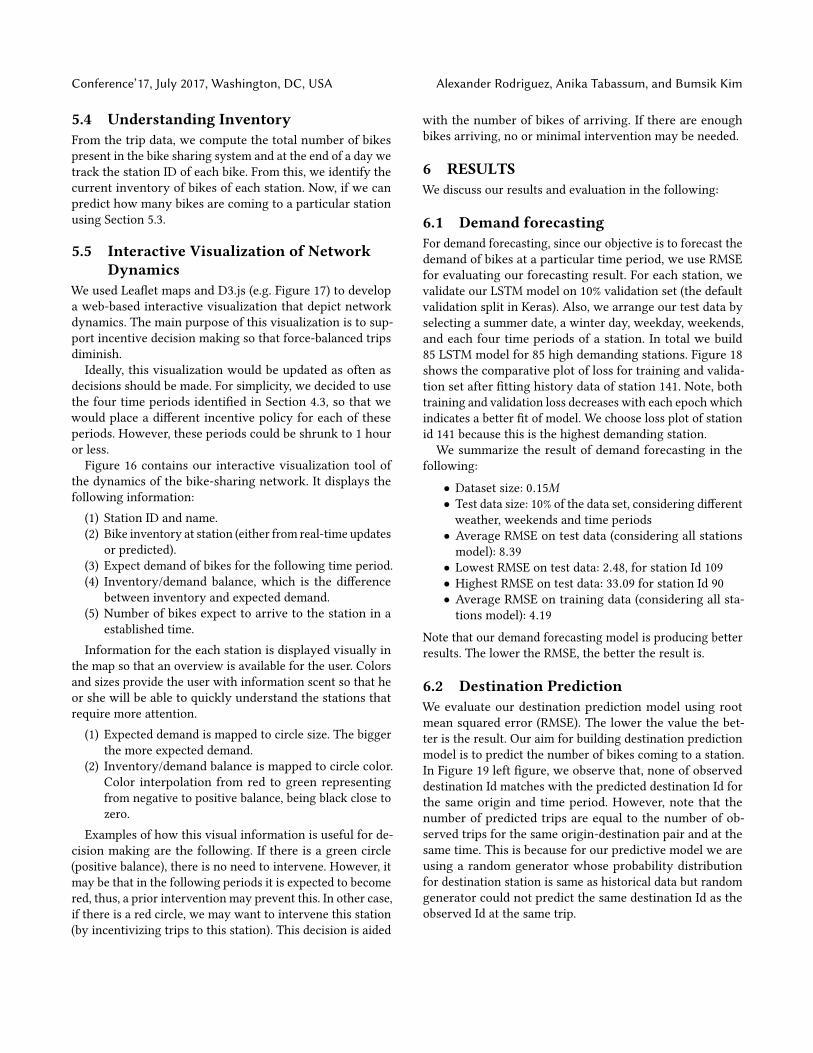
area is selected by census level because the same censuslevel shows similar characteristics. Based on these criteria,we picked census tract that starts their ID as 010, 020, 030,070, 352, and 353. Figure 9 shows the selected station. 85stations are in these area of interest, and we used trip databetween these 85 stations for the analysis.

Figure 9: The selected 85 stations

4.5 Other dataTo enhance the model prediction power, we used additionaldata as our input variables. The authors believe that the mostimportant determinant of biking is weather condition suchas rain and temperature. So we collected one-year weatherdata, includes average temperature, precipitation, snowfall,and wind speed, from the National Oceanic and AtmosphericAdministration (NOAA) and used it as our input variables.Also, we used weekday, weekend, and holiday variables toreflect daily variation. Lastly, we utilized real bike inventorydata to see how many bikes exist by each station.

5 METHODOLOGYThe methodology to understand the dynamics of the sys-tem comprises three parts: detecting force-balanced trips,demand prediction, and destination prediction.

5.1 Detecting force-balanced tripTo detect if a trip or bike needs to be force-balanced is tonecessary to model the decision making of the system. In thefollowing Figure 3 row 3, we observe that a user starts a tripwith a bikeID W00005 from one station (31087) and ends at adifferent station (31047). In row 4, the bikeId W00005 startedtrip from station 31047 to 31083 and it seems reasonablebecause it explains the bike W00005 stayed at station 31047from the end of previous trip. However, in row 5, the bikeId

W00005 started a trip from station 31048 that is supposed tobe the end station (31083) from the previous trip. In this case,the bike W00005 was force-balanced from station 31083 tostation 31048 between 17:56 and 20:29.In this study, we have to know whether this bike needs

to be force-balanced to other station or not and if it needsto be force-balanced then at which hour. For this, we needto know the demand of the station at a particular time fromhistorical data as well as the number of force-balanced tripoccurs at a particular hour of that station.

5.2 Demand ForecastingDemand forecasting or to forecast the demand of bikes of aparticular station of a particular time period of a day can beease the force-balanced decision. We adopted a multivariatetime-series forecasting approach to forecast demand of bikesof a station. We use LSTM sequential model for each stationto forecast demand. We discuss the approach in following:

5.2.1 Data Preprocessing: From Figure. 5 we divide the 24-hour time into four time periods: off peak (8pm-5am), AMpeak (5am-10am), moderate (10am-3pm) and PM peak (3pm-8pm). For each day, We calculate demand of each station atthese four time periods. We assume that, along with timedemand of a station also varies with weather and day of aweek, i.e., demand of a station is different for sunny, rainy,weekdays and holidays. For this, for each trip data, we com-bine the weather variables and holiday variable of that day.Next, among all the stations of one year trip data we select85 high demanding stations as discussed in Sec 4.4. Afterdata preprocessing for each station a row of the dataset hasthe features shown in Table 1. The size of the dataset afterpreprocessing is 0.15M for 85 high demanding stations. Eachstation has on average 1500 index or rows with the followingfeatures as shown in Table 1.

5.2.2 Machine learning model: We use LSTM sequentialmodel for demand forecasting. Our approach is similar tothe multivariate timeseries forecasting1 (MTSF). With giveninput features at time t MTSF forecast features at time t + k .In our case with the input features, i.e., weather variables,holiday or not, time period t and given demand at time pe-riod t our approach forecasts demand for time t + 1. Since,we are using multiple features for forecasting demand alongwith the present time series value, we processed our inputdata to work for supervised learning prediction problem. Fortraining, the LSTM model is based on this- we added onecolumn as output which contains demand at t + 1, i.e., weconsider demand of the same station of the next row in thedataset as our output. For 85 high demanding stations we

1https://machinelearningmastery.com/multivariate-time-series-forecasting-lstms-keras/


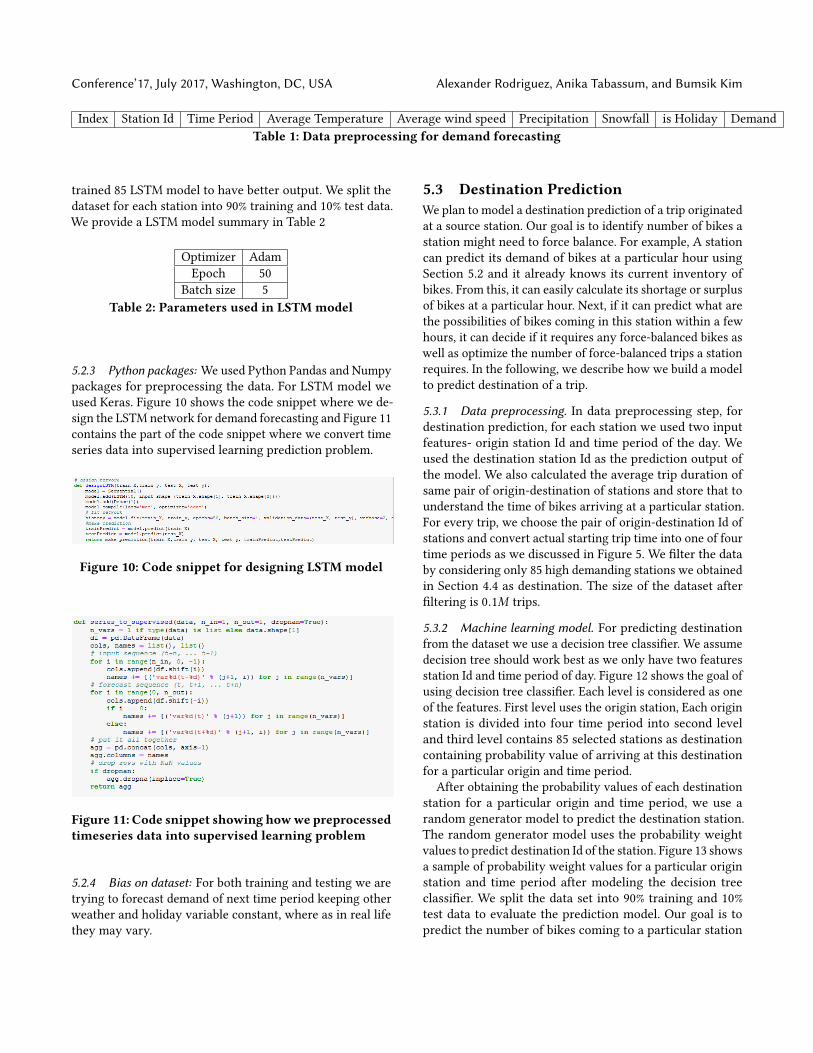
Index Station Id Time Period Average Temperature Average wind speed Precipitation Snowfall is Holiday DemandTable 1: Data preprocessing for demand forecasting

trained 85 LSTM model to have better output. We split thedataset for each station into 90% training and 10% test data.We provide a LSTM model summary in Table 2

Optimizer AdamEpoch 50

Batch size 5Table 2: Parameters used in LSTM model

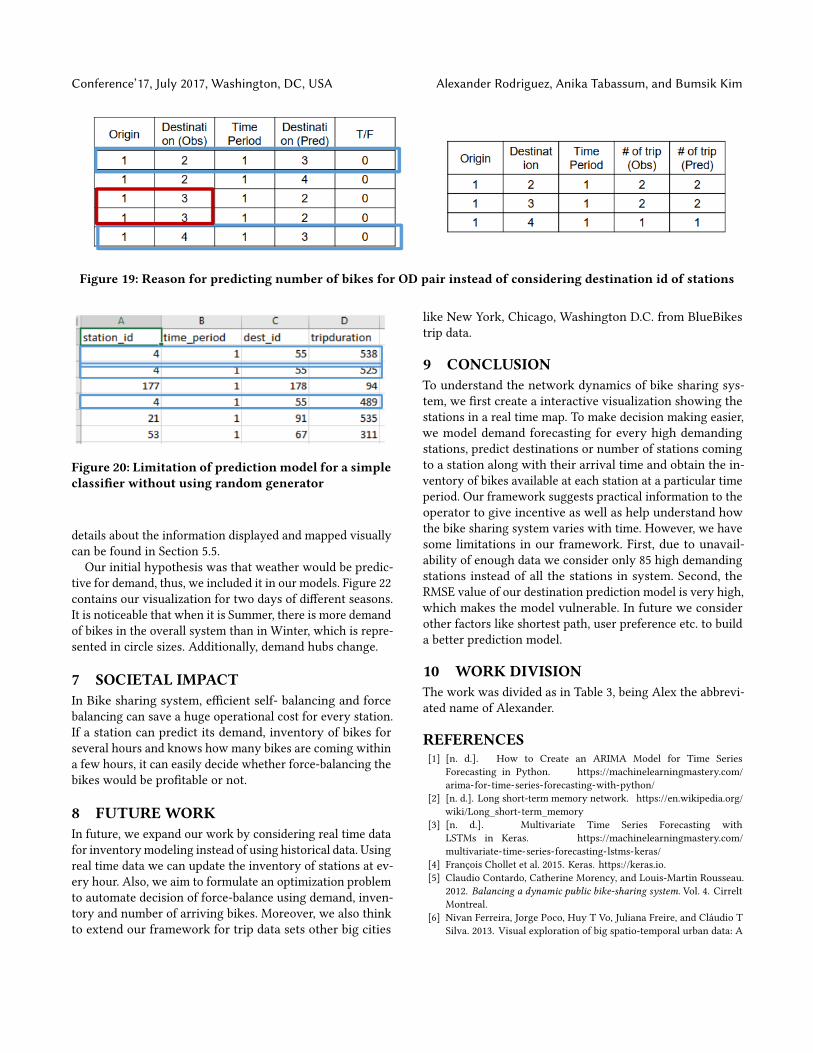
5.2.3 Python packages: We used Python Pandas and Numpypackages for preprocessing the data. For LSTM model weused Keras. Figure 10 shows the code snippet where we de-sign the LSTM network for demand forecasting and Figure 11contains the part of the code snippet where we convert timeseries data into supervised learning prediction problem.

Figure 10: Code snippet for designing LSTM model

Figure 11: Code snippet showing howwe preprocessedtimeseries data into supervised learning problem

5.2.4 Bias on dataset: For both training and testing we aretrying to forecast demand of next time period keeping otherweather and holiday variable constant, where as in real lifethey may vary.

5.3 Destination PredictionWe plan to model a destination prediction of a trip originatedat a source station. Our goal is to identify number of bikes astation might need to force balance. For example, A stationcan predict its demand of bikes at a particular hour usingSection 5.2 and it already knows its current inventory ofbikes. From this, it can easily calculate its shortage or surplusof bikes at a particular hour. Next, if it can predict what arethe possibilities of bikes coming in this station within a fewhours, it can decide if it requires any force-balanced bikes aswell as optimize the number of force-balanced trips a stationrequires. In the following, we describe how we build a modelto predict destination of a trip.

5.3.1 Data preprocessing. In data preprocessing step, fordestination prediction, for each station we used two inputfeatures- origin station Id and time period of the day. Weused the destination station Id as the prediction output ofthe model. We also calculated the average trip duration ofsame pair of origin-destination of stations and store that tounderstand the time of bikes arriving at a particular station.For every trip, we choose the pair of origin-destination Id ofstations and convert actual starting trip time into one of fourtime periods as we discussed in Figure 5. We filter the databy considering only 85 high demanding stations we obtainedin Section 4.4 as destination. The size of the dataset afterfiltering is 0.1M trips.

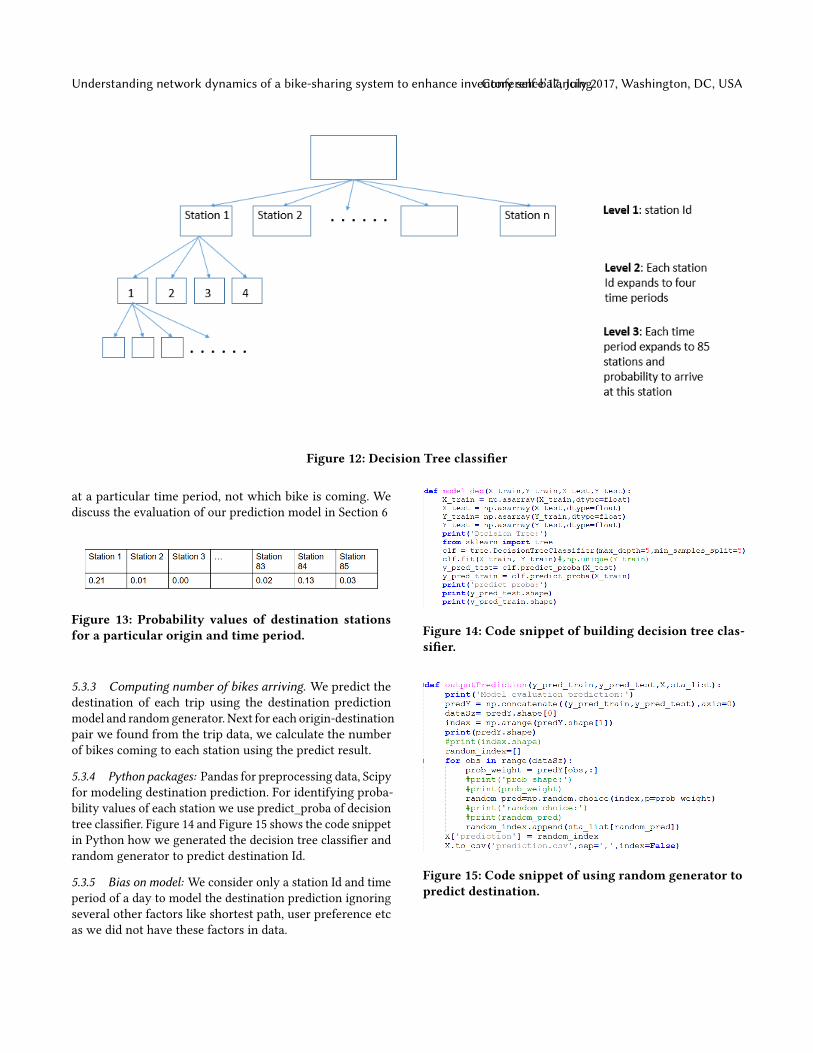
5.3.2 Machine learning model. For predicting destinationfrom the dataset we use a decision tree classifier. We assumedecision tree should work best as we only have two featuresstation Id and time period of day. Figure 12 shows the goal ofusing decision tree classifier. Each level is considered as oneof the features. First level uses the origin station, Each originstation is divided into four time period into second leveland third level contains 85 selected stations as destinationcontaining probability value of arriving at this destinationfor a particular origin and time period.

After obtaining the probability values of each destinationstation for a particular origin and time period, we use arandom generator model to predict the destination station.The random generator model uses the probability weightvalues to predict destination Id of the station. Figure 13 showsa sample of probability weight values for a particular originstation and time period after modeling the decision treeclassifier. We split the data set into 90% training and 10%test data to evaluate the prediction model. Our goal is topredict the number of bikes coming to a particular station


Figure 12: Decision Tree classifier

at a particular time period, not which bike is coming. Wediscuss the evaluation of our prediction model in Section 6

Figure 13: Probability values of destination stationsfor a particular origin and time period.

5.3.3 Computing number of bikes arriving. We predict thedestination of each trip using the destination predictionmodel and randomgenerator. Next for each origin-destinationpair we found from the trip data, we calculate the numberof bikes coming to each station using the predict result.

5.3.4 Python packages: Pandas for preprocessing data, Scipyfor modeling destination prediction. For identifying proba-bility values of each station we use predict_proba of decisiontree classifier. Figure 14 and Figure 15 shows the code snippetin Python how we generated the decision tree classifier andrandom generator to predict destination Id.

5.3.5 Bias on model: We consider only a station Id and timeperiod of a day to model the destination prediction ignoringseveral other factors like shortest path, user preference etcas we did not have these factors in data.

Figure 14: Code snippet of building decision tree clas-sifier.

Figure 15: Code snippet of using random generator topredict destination.


5.4 Understanding InventoryFrom the trip data, we compute the total number of bikespresent in the bike sharing system and at the end of a day wetrack the station ID of each bike. From this, we identify thecurrent inventory of bikes of each station. Now, if we canpredict how many bikes are coming to a particular stationusing Section 5.3.

5.5 Interactive Visualization of NetworkDynamics

We used Leaflet maps and D3.js (e.g. Figure 17) to developa web-based interactive visualization that depict networkdynamics. The main purpose of this visualization is to sup-port incentive decision making so that force-balanced tripsdiminish.Ideally, this visualization would be updated as often as

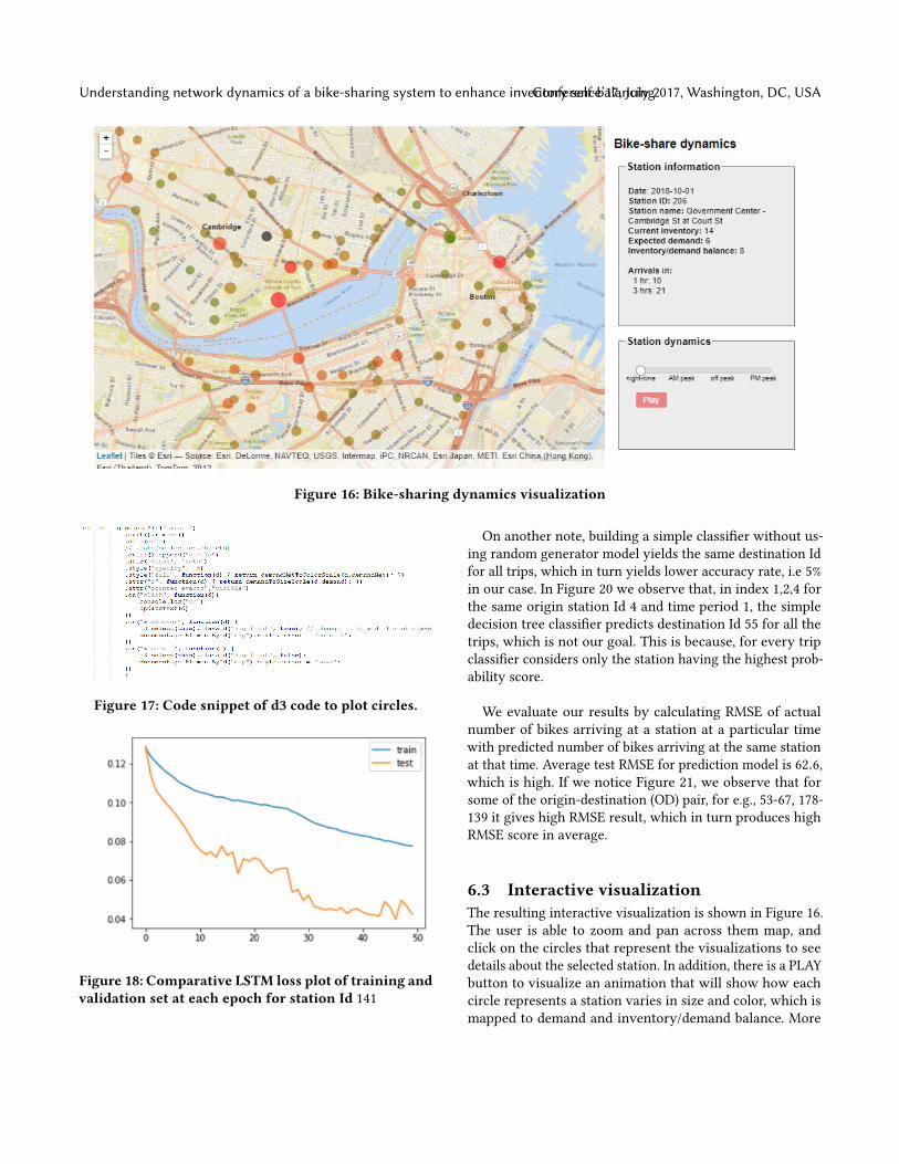
decisions should be made. For simplicity, we decided to usethe four time periods identified in Section 4.3, so that wewould place a different incentive policy for each of theseperiods. However, these periods could be shrunk to 1 houror less.Figure 16 contains our interactive visualization tool of

the dynamics of the bike-sharing network. It displays thefollowing information:(1) Station ID and name.(2) Bike inventory at station (either from real-time updates

or predicted).(3) Expect demand of bikes for the following time period.(4) Inventory/demand balance, which is the difference

between inventory and expected demand.(5) Number of bikes expect to arrive to the station in a

established time.Information for the each station is displayed visually in

the map so that an overview is available for the user. Colorsand sizes provide the user with information scent so that heor she will be able to quickly understand the stations thatrequire more attention.(1) Expected demand is mapped to circle size. The bigger

the more expected demand.(2) Inventory/demand balance is mapped to circle color.

Color interpolation from red to green representingfrom negative to positive balance, being black close tozero.

Examples of how this visual information is useful for de-cision making are the following. If there is a green circle(positive balance), there is no need to intervene. However, itmay be that in the following periods it is expected to becomered, thus, a prior intervention may prevent this. In other case,if there is a red circle, we may want to intervene this station(by incentivizing trips to this station). This decision is aided

with the number of bikes of arriving. If there are enoughbikes arriving, no or minimal intervention may be needed.

6 RESULTSWe discuss our results and evaluation in the following:

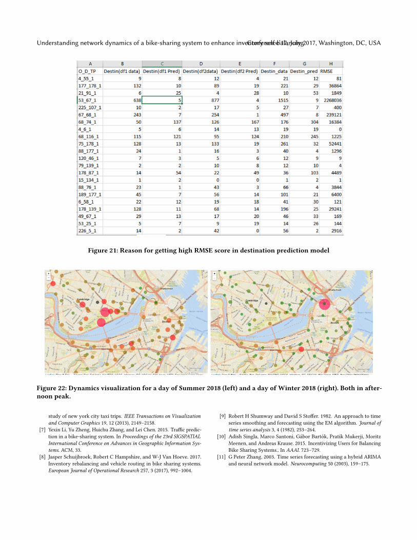
6.1 Demand forecastingFor demand forecasting, since our objective is to forecast thedemand of bikes at a particular time period, we use RMSEfor evaluating our forecasting result. For each station, wevalidate our LSTM model on 10% validation set (the defaultvalidation split in Keras). Also, we arrange our test data byselecting a summer date, a winter day, weekday, weekends,and each four time periods of a station. In total we build85 LSTM model for 85 high demanding stations. Figure 18shows the comparative plot of loss for training and valida-tion set after fitting history data of station 141. Note, bothtraining and validation loss decreases with each epoch whichindicates a better fit of model. We choose loss plot of stationid 141 because this is the highest demanding station.We summarize the result of demand forecasting in the

following:

• Dataset size: 0.15M• Test data size: 10% of the data set, considering differentweather, weekends and time periods

• Average RMSE on test data (considering all stationsmodel): 8.39

• Lowest RMSE on test data: 2.48, for station Id 109• Highest RMSE on test data: 33.09 for station Id 90• Average RMSE on training data (considering all sta-tions model): 4.19

Note that our demand forecasting model is producing betterresults. The lower the RMSE, the better the result is.

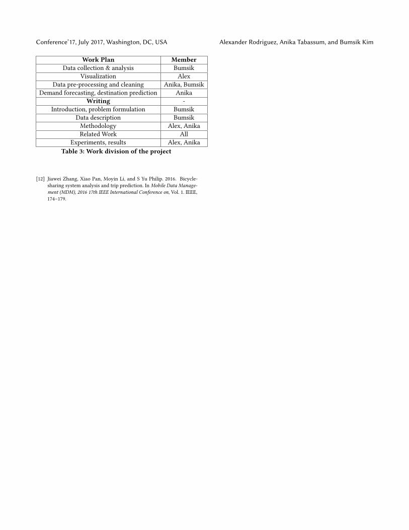
6.2 Destination PredictionWe evaluate our destination prediction model using rootmean squared error (RMSE). The lower the value the bet-ter is the result. Our aim for building destination predictionmodel is to predict the number of bikes coming to a station.In Figure 19 left figure, we observe that, none of observeddestination Id matches with the predicted destination Id forthe same origin and time period. However, note that thenumber of predicted trips are equal to the number of ob-served trips for the same origin-destination pair and at thesame time. This is because for our predictive model we areusing a random generator whose probability distributionfor destination station is same as historical data but randomgenerator could not predict the same destination Id as theobserved Id at the same trip.


Figure 16: Bike-sharing dynamics visualization

Figure 17: Code snippet of d3 code to plot circles.

Figure 18: Comparative LSTM loss plot of training andvalidation set at each epoch for station Id 141

On another note, building a simple classifier without us-ing random generator model yields the same destination Idfor all trips, which in turn yields lower accuracy rate, i.e 5%in our case. In Figure 20 we observe that, in index 1,2,4 forthe same origin station Id 4 and time period 1, the simpledecision tree classifier predicts destination Id 55 for all thetrips, which is not our goal. This is because, for every tripclassifier considers only the station having the highest prob-ability score.

We evaluate our results by calculating RMSE of actualnumber of bikes arriving at a station at a particular timewith predicted number of bikes arriving at the same stationat that time. Average test RMSE for prediction model is 62.6,which is high. If we notice Figure 21, we observe that forsome of the origin-destination (OD) pair, for e.g., 53-67, 178-139 it gives high RMSE result, which in turn produces highRMSE score in average.

6.3 Interactive visualizationThe resulting interactive visualization is shown in Figure 16.The user is able to zoom and pan across them map, andclick on the circles that represent the visualizations to seedetails about the selected station. In addition, there is a PLAYbutton to visualize an animation that will show how eachcircle represents a station varies in size and color, which ismapped to demand and inventory/demand balance. More


Figure 19: Reason for predicting number of bikes for OD pair instead of considering destination id of stations

Figure 20: Limitation of predictionmodel for a simpleclassifier without using random generator

details about the information displayed and mapped visuallycan be found in Section 5.5.

Our initial hypothesis was that weather would be predic-tive for demand, thus, we included it in our models. Figure 22contains our visualization for two days of different seasons.It is noticeable that when it is Summer, there is more demandof bikes in the overall system than in Winter, which is repre-sented in circle sizes. Additionally, demand hubs change.

7 SOCIETAL IMPACTIn Bike sharing system, efficient self- balancing and forcebalancing can save a huge operational cost for every station.If a station can predict its demand, inventory of bikes forseveral hours and knows how many bikes are coming withina few hours, it can easily decide whether force-balancing thebikes would be profitable or not.

8 FUTUREWORKIn future, we expand our work by considering real time datafor inventorymodeling instead of using historical data. Usingreal time data we can update the inventory of stations at ev-ery hour. Also, we aim to formulate an optimization problemto automate decision of force-balance using demand, inven-tory and number of arriving bikes. Moreover, we also thinkto extend our framework for trip data sets other big cities

like New York, Chicago, Washington D.C. from BlueBikestrip data.

9 CONCLUSIONTo understand the network dynamics of bike sharing sys-tem, we first create a interactive visualization showing thestations in a real time map. To make decision making easier,we model demand forecasting for every high demandingstations, predict destinations or number of stations comingto a station along with their arrival time and obtain the in-ventory of bikes available at each station at a particular timeperiod. Our framework suggests practical information to theoperator to give incentive as well as help understand howthe bike sharing system varies with time. However, we havesome limitations in our framework. First, due to unavail-ability of enough data we consider only 85 high demandingstations instead of all the stations in system. Second, theRMSE value of our destination prediction model is very high,which makes the model vulnerable. In future we considerother factors like shortest path, user preference etc. to builda better prediction model.

10 WORK DIVISIONThe work was divided as in Table 3, being Alex the abbrevi-ated name of Alexander.

REFERENCES[1] [n. d.]. How to Create an ARIMA Model for Time Series

Forecasting in Python. https://machinelearningmastery.com/arima-for-time-series-forecasting-with-python/

[2] [n. d.]. Long short-term memory network. https://en.wikipedia.org/wiki/Long_short-term_memory

[3] [n. d.]. Multivariate Time Series Forecasting withLSTMs in Keras. https://machinelearningmastery.com/multivariate-time-series-forecasting-lstms-keras/

[4] François Chollet et al. 2015. Keras. https://keras.io.[5] Claudio Contardo, Catherine Morency, and Louis-Martin Rousseau.

2012. Balancing a dynamic public bike-sharing system. Vol. 4. CirreltMontreal.

[6] Nivan Ferreira, Jorge Poco, Huy T Vo, Juliana Freire, and Cláudio TSilva. 2013. Visual exploration of big spatio-temporal urban data: A

https://machinelearningmastery.com/arima-for-time-series-forecasting-with-python/

https://machinelearningmastery.com/arima-for-time-series-forecasting-with-python/

https://en.wikipedia.org/wiki/Long_short-term_memory

https://en.wikipedia.org/wiki/Long_short-term_memory

https://machinelearningmastery.com/multivariate-time-series-forecasting-lstms-keras/

https://machinelearningmastery.com/multivariate-time-series-forecasting-lstms-keras/

https://keras.io


Figure 21: Reason for getting high RMSE score in destination prediction model

Figure 22: Dynamics visualization for a day of Summer 2018 (left) and a day of Winter 2018 (right). Both in after-noon peak.

study of new york city taxi trips. IEEE Transactions on Visualizationand Computer Graphics 19, 12 (2013), 2149–2158.

[7] Yexin Li, Yu Zheng, Huichu Zhang, and Lei Chen. 2015. Traffic predic-tion in a bike-sharing system. In Proceedings of the 23rd SIGSPATIALInternational Conference on Advances in Geographic Information Sys-tems. ACM, 33.

[8] Jasper Schuijbroek, Robert C Hampshire, and W-J Van Hoeve. 2017.Inventory rebalancing and vehicle routing in bike sharing systems.European Journal of Operational Research 257, 3 (2017), 992–1004.

[9] Robert H Shumway and David S Stoffer. 1982. An approach to timeseries smoothing and forecasting using the EM algorithm. Journal oftime series analysis 3, 4 (1982), 253–264.

[10] Adish Singla, Marco Santoni, Gábor Bartók, Pratik Mukerji, MoritzMeenen, and Andreas Krause. 2015. Incentivizing Users for BalancingBike Sharing Systems.. In AAAI. 723–729.

[11] G Peter Zhang. 2003. Time series forecasting using a hybrid ARIMAand neural network model. Neurocomputing 50 (2003), 159–175.


Work Plan MemberData collection & analysis Bumsik

Visualization AlexData pre-processing and cleaning Anika, Bumsik

Demand forecasting, destination prediction AnikaWriting -

Introduction, problem formulation BumsikData description BumsikMethodology Alex, AnikaRelated Work All

Experiments, results Alex, AnikaTable 3: Work division of the project

[12] Jiawei Zhang, Xiao Pan, Moyin Li, and S Yu Philip. 2016. Bicycle-sharing system analysis and trip prediction. In Mobile Data Manage-ment (MDM), 2016 17th IEEE International Conference on, Vol. 1. IEEE,174–179.

Documents

Understanding network dynamics of a bike-sharing system to