Embed Size (px)
Citation preview
Florida International UniversityFIU Digital Commons
FIU Electronic Theses and Dissertations University Graduate School
11-14-2014
Understanding Immigrants' Travel Behavior inFlorida: Neighborhood Effects and BehavioralAssimilationNishat [email protected]
DOI: 10.25148/etd.FI14110770Follow this and additional works at: https://digitalcommons.fiu.edu/etd
Part of the Civil Engineering Commons, Other Civil and Environmental Engineering Commons,Urban, Community and Regional Planning Commons, and the Urban Studies and PlanningCommons
This work is brought to you for free and open access by the University Graduate School at FIU Digital Commons. It has been accepted for inclusion inFIU Electronic Theses and Dissertations by an authorized administrator of FIU Digital Commons. For more information, please contact [email protected].
Recommended CitationZaman, Nishat, "Understanding Immigrants' Travel Behavior in Florida: Neighborhood Effects and Behavioral Assimilation" (2014).FIU Electronic Theses and Dissertations. 1690.https://digitalcommons.fiu.edu/etd/1690
FLORIDA INTERNATIONAL UNIVERSITY
Miami, Florida
UNDERSTANDING IMMIGRANTS’ TRAVEL BEHAVIOR IN FLORIDA:
NEIGHBORHOOD EFFECTS AND BEHAVIORAL ASSIMILATION
A thesis submitted in partial fulfillment of
the requirements for the degree of
MASTER OF SCIENCE
in
CIVIL ENGINEERING
by
Nishat Zaman
2014
ii
To: Dean Amir Mirmiran choose the name of dean of your college/school College of Engineering and Computing choose the name of your college/school
This thesis, written by Nishat Zaman, and entitled Understanding Immigrants’ Travel Behavior in Florida: Neighborhood Effects and Behavioral Assimilation, having been approved in respect to style and intellectual content, is referred to you for judgment.
We have read this thesis and recommend that it be approved.
_______________________________________ L. David Shen
_______________________________________
Albert Gan
_______________________________________ Mohammed Hadi
_______________________________________
Xia Jin, Major Professor
Date of Defense: November 14, 2014
The thesis of Nishat Zaman is approved.
_______________________________________ choose the name of dean of your college/school Dean Amir Mirmiran
choose the name of your college/school College of Engineering and Computing
______________________________________ Dean Lakshmi N. Reddi
University Graduate School
Florida International University, 2014

iii
© Copyright 2014 by Nishat Zaman
All rights reserved.
iv
DEDICATION
My Husband, Dr. Iftheker A. Khan
My Parents, Dr. S. M. Wahiduzzaman and Mrs. M. Z. Jesmin Ferdous
My Brother, Mr. Nur-E-Zaman Ayshik

v
ACKNOWLEDGMENTS
I gratefully acknowledge the role of Dr. Xia Jin, Assistant Professor of Civil and
Environmental Engineering at Florida International University (FIU), as my research
advisor in my current program of study. Her guidance, support, and inspiration have
helped me complete my degree. I am sincerely indebted to her for everything I have
learned, both academic and non-academic. Her calm, friendly, and kind demeanor were
indispensable and helped me survive the difficult days away from my family and home
country, Bangladesh. Dr. Jin accepted all of my shortcomings yet always gave me the
opportunity to explore my ideas outside the box. Her methods of disseminating research
and passionate teaching are very best I have ever experienced. I find myself very
fortunate to be part of her enthusiastic research group.
I am very thankful to Dr. L. David Shen, Dr. Mohammed Hadi, and Dr. Albert
Gan for guiding me in thesis preparation and serving as thesis committee members
despite their busy schedules. I remember the day when I received my acceptance for
admission from Graduate Program Director Dr. Shen. It was just the beginning of the
endless support I have received over the years from him. I am proud to have worked as a
graduate research assistant at the Lehman Center for Transportation Research (LCTR) at
FIU. I am indebted to Dr. Hadi for his valuable assessments and inspiration to complete
the thesis work, and for his guidance on how to lead the Institute of Transportation
Engineers (ITE) Student Chapter at FIU. It was a special privilege to find myself under
the protective care of Dr. Gan in various occasions, both academic and personal. I am
also thankful to Dr. Giri Narasimhan, Associate Dean of Research and Graduate Studies

vi
in the College of Engineering and Computing at FIU, for encouraging me to extend my
research beyond the current program.
I sincerely acknowledge my undergraduate mentor Professor Suman K. Mitra of
the Dept. of Urban and Regional Planning at Bangladesh University of Engineering and
Technology, for his encouragement and guidance in graduate education. I am thankful to
my husband Dr. Iftheker A. Khan; my parents, Dr. S. M. Wahiduzzaman and Mrs. M. Z.
Jesmin Ferdous; my brother, Mr. Nur-E-Zaman Ayshik; my father- and mother-in-law,
Mr. Nizam A. Khan and Mrs. Badrun N. Begum; my sisters-in-law, Mrs. Naznin
Khanom and Ms. Hafsa Khanom; my lifetime inspiration Apuli; my loving Tuktuki and
Aourthy; my greatest hero, Baven Rizvan; and my best friends forever, Sifat, Sutapa,
Tanjila, Shatabdi, Dibanur, Leeoza, Ananya, Shazia, Nazia, Chaity, Tasneem, and Naba,
for showing immense support and relentless love toward the fulfillment of my dream.
My heartfelt thanks goes to my research colleagues, Mr. Hamidreza Asgari, for
his continued help and invaluable insight in model development; Mr. Kollol Shams for
guidance in GIS works; Mr. Sakoat Hossan for his great inspiration; Mr. Zhaohan Zhang
and Mr. Fengjiang Hu for their brotherly care; and Mr. Mario Rojas and Mr. Mohammad
Lavasani for always being friendly. I am thankful to Mr. Dibakar Saha for his endless
support over the years in both my academic and personal issues. I am thankful to my very
near and dear friends, Ms. Samaneh Khazraeian, Mr. Shahadat Iqbal, Mr. Aidin Massahi,
Mr. Xuanwu Chen, Mr. Revanth Redla and Mr. Asif Raihan for their immense support. I
acknowledge the Department of Civil and Environmental Engineering at FIU for
providing me with the curricular and research framework, and the financial assistance for
the entire program of study.

vii
ABSTRACT OF THE THESIS
UNDERSTANDING IMMIGRANTS’ TRAVEL BEHAVIOR IN FLORIDA:
NEIGHBORHOOD EFFECTS AND BEHAVIORAL ASSIMILATION
by
Nishat Zaman
Florida International University, 2014
Miami, Florida
Professor Xia Jin, Major Professor
The goal of this study was to develop Multinomial Logit models for the mode
choice behavior of immigrants, with key focuses on neighborhood effects and behavioral
assimilation. The first aspect shows the relationship between social network ties and
immigrants’ chosen mode of transportation, while the second aspect explores the gradual
changes toward alternative mode usage with regard to immigrants’ migrating period in
the United States (US). Mode choice models were developed for work, shopping, social,
recreational, and other trip purposes to evaluate the impacts of various land use patterns,
neighborhood typology, socioeconomic-demographic and immigrant related attributes on
individuals’ travel behavior. Estimated coefficients of mode choice determinants were
compared between each alternative mode (i.e., high-occupancy vehicle, public transit,
and non-motorized transport) with single-occupant vehicles. The model results revealed
the significant influence of neighborhood and land use variables on the usage of
alternative modes among immigrants. Incorporating these indicators into the demand
forecasting process will provide a better understanding of the diverse travel patterns for
the unique composition of population groups in Florida.
viii
TABLE OF CONTENTS
CONTENT PAGE
1. INTRODUCTION ...................................................................................................... 1 1.1. Motivation ............................................................................................................ 1 1.2. Goals and Objectives ............................................................................................ 2 1.3. Contribution ......................................................................................................... 3 1.4. Thesis Organization .............................................................................................. 4
2. LITERATURE REVIEW ........................................................................................... 5 2.1. Immigrant Travel Behavior .................................................................................. 5 2.2. Land Use Impacts on Travel Behavior ................................................................. 8 2.3. Neighborhood Effects ........................................................................................ 11 2.4. Modeling Approaches of Immigrant Travel Patterns ......................................... 16 2.5. Limitations That This Study Covers .................................................................. 21 2.6. Summary ............................................................................................................ 22
3. DATA AND DESCRIPTIVE ANALYSIS .............................................................. 23 3.1. Derivation of Land Use Variables ...................................................................... 24 3.2. Determination of Neighborhood Effects ............................................................ 29 3.3. Behavioral Assimilation Analysis ...................................................................... 42 3.4. Summary ............................................................................................................ 52
4. METHODOLOGY ................................................................................................... 53 4.1. Hypothesis .......................................................................................................... 53 4.2. Model Structure .................................................................................................. 53
5. RESULTS AND DISCUSSIONS ............................................................................. 56 5.1. Individual Attributes .......................................................................................... 69 5.2. Household Attributes.......................................................................................... 71 5.3. Immigrant-related Attributes .............................................................................. 73 5.4. Land Use Attributes ........................................................................................... 74 5.5. Neighborhood Attributes .................................................................................... 75 5.6. Summary ............................................................................................................ 77
6. CONCLUSION AND RECOMMENDATIONS ..................................................... 78 6.1. Conclusion .......................................................................................................... 78 6.2. Recommendations .............................................................................................. 81
REFERENCES ................................................................................................................. 82

ix
LIST OF TABLES
TABLE PAGE
Table 1. Grouping of LEHD Origin-Destination Employment Statistics (LODES) Work
Area Characteristics CNS Fields to Support Five-tier Mix Variable. .............................. 28
Table 2. Tracts Based on Location Quotient Value of Immigrant Concentration. ........... 31
Table 3. Communalities and Orthogonal Varimax Rotation Matrix of Extended Factors.
........................................................................................................................................... 36
Table 4. Eigenvalues Indicating the Cumulative Percentage of Explained Variance. ...... 37
Table 5. Rotated Factor Loading Pattern of the Neighborhood Social Characteristics. ... 38
Table 6. Distribution of Census Tracts under Two Neighborhood Factors. ..................... 40
Table 7. Determinants of Mode Choice Model Outcome for Work Trips. ....................... 57
Table 8. Determinants of Mode Choice Model Outcome for Shopping Trips. ................ 60
Table 9. Determinants of Mode Choice Model Outcome for Social and Recreational
Trips. ................................................................................................................................. 63
Table 10. Determinants of Mode Choice Model Outcome for Other Trips. ..................... 66
x
LIST OF FIGURES
FIGURE PAGE
Figure 1. Q-Q Plot for (a) Factor 1 and (b) Factor 2 Scores. ............................................ 34
Figure 2. Scree Plot Showing Eigenvalues for Chosen Components. .............................. 37
Figure 3. Perceptual Map of Neighborhood Social Context. ............................................ 39
Figure 4. Distribution of Neighborhood Typologies throughout the Florida State. ......... 41
Figure 5. Change in Immgrant Households Race/Ethnicity Share with respect to Arrival
Time in the US. ................................................................................................................. 43
Figure 6. Change in Household Life Cycle Scenario ....................................................... 45
Figure 7. Comparison of Household Size between Foreign-born and US-born
Households. ....................................................................................................................... 46
Figure 8. Distribution of Immigrants Household Size over their Migrating Period in the
US. .................................................................................................................................... 46
Figure 9. Change in Household Yearly Income of the Foreign-born Households over
Their Migration Period in the US. .................................................................................... 48
Figure 10. Comparison of Household Vehicles between Foreign-born and US-born. ..... 49
Figure 11. Change in Number of Households Vechicle(s) Ownership of Immigrants over
Their Migration Period in the US. .................................................................................... 49
Figure 12. Change in Home Ownership Pattern over the Years for Immigrants. ............. 50
Figure 13. Change in Type of Household over the Years for Immigrants. ...................... 51
xi
LIST OF ACRONYMS AND ABBREVIATIONS
NHTS National Household Travel Survey
ACS American Community Survey
US United States
EPA Environmental Protection Agency
PUMA Public Use Micro-data Areas
MNL Multinomial Logit
NL Nested Logit
SED Socio-economic Demographics
IIA Independence of Irrelevant Alternatives
VMT Vehicle Miles Traveled
SOV Single-Occupant Vehicles
HOV High-Occupancy Vehicle
PCA Principal Component Analysis
KMO Kaiser-Meyer-Olkin
MSA Measure of Sampling Adequacy
NMT Non-Motorized Transport
1
1. INTRODUCTION
1.1. Motivation
Aside from Australia and Canada, the United States (US) is a popular hosting country for
immigrants [1]. Foreign-born individuals, other than those who have US-born parents, are
considered immigrants [2]. Between 1990 and 2010, immigrants and their children and
grandchildren accounted for half of the total population increase in the US [3].
Specifically, the immigrant population accounted for 13% of the total US population and
16.4% of the workers engaged in the US civilian labor force in 2012 [4]. These
immigrants vitalize the country’s overall population growth, cultural versatilities,
settlement pattern changes, and economic paradigm shift. Given the significant
contributions of immigrants to the demographic, social, economic, and cultural aspects of
the country, many researchers have studied immigrants’ housing, health, education, and
employment conditions. However, the transportation aspects for immigrants, especially
their attitude towards different travel modes and choices, have not received as much
attention.
Research to date suggests that immigrants reveal aberrant travel behavior in
comparison to US-born residents, and they have a higher usage of transit, carpool, and
non-motorized modes [5-8]. Much remains unexplored in terms of the underlying factors
and the transferability of their impact, which leads to the higher usage of alternative
modes among immigrants. These factors may involve cultural preferences related to
social network and lifestyle, such as larger households, close coordination among
household members and friends, and living in dense or mixed-use neighborhoods. Other
2
factors, e.g., lower car ownership and legal barriers, may be more passive. As the third
largest and the seventh fastest growing state in the country, Florida witnessed an
unprecedented wave of immigration from abroad, especially the Caribbean and Latin
America, in the past several decades. The foreign-born population made up 19.4% of the
total population in Florida in 2012 [9], and they represent almost one-quarter of the entire
workforce of Florida [10]. Therefore, it is critical for planning agencies to understand this
population’s travel behavior for today’s transportation decisions, and all the more so to
understand the implications of the succeeding generations in shaping future travel
patterns to promote sustainable and livable transportation in Florida.
1.2. Goals and Objectives
The goal of this research is to develop econometric models to investigate the mode choice
behavior of immigrants by considering two major aspects, i.e., neighborhood effect and
behavioral assimilation. Neighborhood effect is the combined effect of people’s personal
and household backgrounds, and their interaction with those living in the nearby (or
common) area or that have similar racial/ethnic identity. It is hypothesized that this effect
is inherent in people’s social ties rather than defined by a geographic boundary, and has a
significant impact on immigrants’ mode choice behavior. Behavioral assimilation
examines the residual impact that remains after immigrants acculturate into the American
lifestyle. It is hypothesized that this characteristic is reflected both through their
residential self-selection and travel mode choice. More specifically, the research
questions to be answered through this study include the following:

3
1. Does living in an immigrant neighborhood lead to a higher usage of alternative
modes for immigrants while controlling relevant factors (e.g., density, size, and
other land use variables)?
2. Is the level of preference toward transit and non-motorized modes associated with
the number of years immigrants lived in the US while controlling relevant factors
(e.g., income, household lifecycle, auto ownership, etc.)?
The first question focuses on the neighborhood or agglomeration effects, beyond
what is being generally considered built environment factors that contribute to the use of
transit and non-motorized modes. The second question examines to what degree the
effect of being an immigrant on the use of alternative modes remains or disappears as
they settle in, regardless of other potential correlated changes in the household, such as
income levels, household lifecycle, and auto ownership. By considering both aspects,
econometric models will be developed to determine relevant immigrant indicators.
1.3. Contribution
Incorporating immigrant indicators into the demand forecasting process enhances the
performance of the mode choice models to better reflect the diverse travel patterns of the
unique demographics in Florida. This study will provide better tools to facilitate policy
and investment decisions to meet the travel needs for immigrant communities and inform
the efforts in promoting sustainable transportation system. Furthermore, the study
approach and research results will have broader impacts and applicability to other
regions, thereby helping state, regional, and local agencies to better understand the travel
behavior and transportation needs for immigrants.
4
1.4. Thesis Organization
The organization of this thesis follows a logical sequence of studying neighborhood
effects and behavioral assimilation in immigrants’ travel behavior in Florida. Chapter 1
introduces the motivation, overall objectives, and contribution of the thesis. Chapter 2
presents literature on the travel behavior of immigrants in the US and how built-in
environments impact travel behavior. In addition, it includes current literature on
neighborhood effects from both social science and transportation engineering
perspectives. Moreover, the modeling approaches of immigrant travel behavior, with a
key focus on mode choice modeling approaches, are also discussed. Chapter 3 discusses
the data sources and their use in the descriptive and statistical analyses. The detailed
description used to obtain the land use and neighborhood attributes and corresponding
data processing method allows readers to understand the entire engineering of available
data based on the requirements of the models. Moreover, it includes the statistical
analysis to validate the inclusion of residence time in the mode choice model. Chapter 4
presents the Multinomial Logit Model structure that incorporates variables capturing
socio-economic demographic characteristics, land use pattern, neighborhood attributes,
individuals’ immigrant status and their behavioral assimilation trend. Chapter 5 presents
determinants of the mode choice model outcome for work, shopping, social, recreational,
and other trip purposes. The results are summarized and individuals’ particular mode
choice(s) are discussed in details. The final chapter, Chapter 6, presents key findings and
accomplishment of the thesis along with suggestions in specific areas for future research.
5
2. LITERATURE REVIEW
Travel patterns vary on the basis of people, culture, geographic characteristics, etc. [11].
Similarly, a travel pattern is an indicator of people’s preferences and habits, availability
of opportunities, and the transportation constraints encountered [12]. Moreover, people of
different occupations, attitudes, and lifestyles possess different types of travel behavior
[13, 14]. Travel behavior of any specific population group is defined as the window that
shows the lives of individuals within that group [14]. Therefore, any kind of policy
planning or decision-making process regarding transportation issues related to that
specific group requires insight on travel patterns and underlying factors.
2.1. Immigrant Travel Behavior
Immigrants in the US are people of versatile races/ethnicities that have a wide gamut of
cultures and lifestyles as they come from various parts of the world, and have a complex
combination of travel behaviors. A previous study on immigrants in a California region
showed that people of various nationalities had preferences toward different travel modes
despite being in the same geographic area and having similar economic backgrounds
[15]. South Asians are linguistically isolated from other ethnic groups in this region,
choosing to avoid public transportation, while immigrants from China, Vietnam, and
Laos prefer privacy and tend to buy automobiles at higher rate. This proves that cultural
complexities affect estimations of how people travel and make trips. In the previous
decade or so researchers have focused on identifying the travel behavior of the
immigrants in different ways. Researchers explore immigrants’ travel behaviors from
various points of view that reflect versatile dimensions of their livelihood. The following
6
section provides a glimpse of immigrants’ travel patterns that have been derived by
studies to date.
Researchers sketch an outline immigrant travel behaviors by comparing
immigrants with the US-born population. Most of the previous studies reveal that
immigrants are more inclined toward the use of alternative modes, i.e., carpooling, ride
sharing, public transit, walking, and biking, than US-born individuals [12, 14, 16-19].
There are various opportunities that allow immigrants to survive with the use of
alternative travel modes. In addition, there are constraints that make private vehicle
ownership unattainable.
In comparison to the US-born population, immigrants generally live in
neighborhoods with higher residential and employment densities where destinations are
reachable by shorter walking or biking trips [14, 16, 17], or in dense urban
neighborhoods with extensive transit service [19]. In general, immigrants reside in
metropolitan areas at a rate of twice than the US-born [12]. During their migration stage,
immigrants choose these housing locations based on income, household sizes, etc., and
settle down in these inner city enclaves of disadvantaged areas where the majority of
people with limited socio-economic resources reside [20].
Immigrants face linguistic and driving license constraints, higher auto insurance
rates, and the financial inability to afford a private vehicle at early stages of migration to
the US [15, 17]. Even if they possess automobiles, in almost all cases, these are found to
be old model vehicles of more troublesome maintenance. This leads immigrants to rely
on other options, e.g., carpooling and ride sharing. They maintain a social network as a
valuable and more accessible source for these types of private transportation. This
7
supports the analogy of living in clusters of ethnic people [21]. The idea of social
network has effectively taken place for both immigrant and non-immigrant
neighborhoods in the form of social ties. This drives immigrants toward more alternative
types of mode usage than the US-born populace. However, the proportion of using
alternative modes is higher within immigrant neighborhoods than non-immigrant
neighborhoods. The existence of social ties was demonstrated earlier by developing a
Multinomial Logit (MNL) mode choice model [14].
Living in the same or nearby ethnic neighborhood makes it favorable for
immigrants to choose alternative transportation, such as carpooling, car-borrowing, or
ride-sharing, from the social network. Factors like spatial proximity, temporal
compatibility, and no time overlapping play significant roles in the likelihood of
receiving transportation support [22]. This comes with an opportunity to interact with job
providers. It is reported that oftentimes, immigrants are employed within co-ethnic
businesses [21]. An earlier study explored the mode choice pattern of immigrants from
ethnic enclaves and ethnic niches using Residential and Industrial location quotients,
respectively [18]. The significant impacts of the circumstance of living in an ethnic
enclave or working in an ethnic niche on carpooling and public transit usage were shown.
The results differed greatly from that of the non-enclave residents and non-niche workers.
Moreover, it was found that working in these ethnic niches generated more interest in
living in the ethnic enclaves. These are potential sources of information flow regarding
opportunities for newcomers. These groups of individuals are more likely to use
alternative modes of transportation. All of these studies and facts expose the immigrants’
household location choice as a pervasive aspect of their travel behavior.

8
Several studies relate immigrants’ duration of living in the US as a positive
influence over their economic and social conditions [15]. The immigrants gain the
economic similarity of middle-income Americans after living more than thirty years in
the US [21]. The vehicle-ride lenders that lend to new immigrants in the ethnic social
networks are usually those who are already economically established and have been
living for a substantially longer period of time in the US [22]. New immigrants usually
have a long-term plan to own private vehicles, and in the interim, they have the ability to
personalize the idea of owning and maintaining their own private vehicles.
Immigrants’ household characteristics, both from geographic and demographic
aspects, change over their migration period and impact their travel patterns. In the case of
geographic dimension, immigrants tend to navigate within better neighborhoods of
residential amenities. They experience social mobility and become acculturated in the
mainstreaming lifestyles of US-born Americans [20]. Moreover, the development of their
economic condition broadens their outlook [23]. In demographic features, most of the
newer immigrants possess smaller families and have fewer propensities to drive alone
than those who have been in the US for more than 10 years [17, 18]. However, with the
passage of time, their families increase with the birth of children, necessitating more trips
and moving forward to own private vehicles [17]. Therefore, the duration of living in the
US has a significant impact on an immigrant’s economic and household status.
2.2. Land Use Impacts on Travel Behavior
Immigrants’ travel patterns are revealed by their preference toward different residential
locations. At different stages of settlement, they change their residential location; this fact

9
shapes their travel behavior dynamically [20]. Land use pattern and household
composition are indicators of residential/household location choice, which is labeled as
the primary determinant of individuals’ mode choice behavior [24]. Conceptual
Structural Equation Model (SEM) was reported earlier for this purpose [13]. In
subsequent chapters, the aspects of a residential location that make people’s travel
behavior different will be discussed. In addition, built environment characteristics that
attract people to live within a specific location for better access to more convenient
transportation modes will be examined.
Mode choice and departure time determine the efficiency of the whole
transportation system, as these are the most important components of travel behavior.
Travel behavior and residential location have a significant and lasting impact in terms of
changing urban form, land use, and transportation patterns. To explore the relationship
among residential locations, mode choice, and departure time, a previous study was
conducted on eight Chinese administrative districts by formulating joint choice sets using
both the Cross-Nested and traditional Nested Logit Model [25]. The model was
formulated based on the random utility maximization theory by taking into consideration
an individual’s house price, travel time, travel cost, and socio-economic characteristics as
exogenous variables [25]. In addition, the model choice sets combined the house location,
travel time, and mode choice variables as the subsets. The result showed that the decision
makers would first change their departure time, then choice of mode, and finally
residential location. For example, the increase in travel time persuades travelers to change
their departure time and travel mode, rather than residential location. Analysis of direct
elasticity suggests that in the case of long distance commuting, it is difficult to reduce car

10
usage, even if a higher charge is imposed, whereas public transit users are more sensitive
to travel costs.
An individual’s travel behavior, including mode choice, vehicle miles traveled,
and auto-ownership, vary on land use patterns [26]. Areas of mixed land use provide
more accessibility to opportunities, thereby resulting in shorter trip distances. This fact
encourages people to drive less and use alternative modes in higher magnitudes,
compared to solo driving. These areas are associated with higher land prices, congestion,
and a reduced amount of parking availability [11, 27, 28]. Similarly, the presence of rail
stations within PUMA increase the likelihood of transit usage [18]. This collaborates with
job and population density as determinants of auto-ownership status [24, 28].
A previous study examined the impact of built environments, transportation
network attributes, and demographic characteristics on residential choice and car
ownership decisions from a joint mixed Multinomial Logit-ordered response structure
[24]. The model structure includes the residential self-selection effect into neighborhood
as a control to testify the effects of built environment attributes on choices related to
travel behavior related choices specifically car ownership. Moreover, people’s
demographic attributes, along with unobserved household factors, were added to reflect
differential sensitivity. Households with seniors, middle- and higher-income residents,
low-income residents, and single families prefer locations of less density and population
clustering, less employment-dense areas, employment-dense areas, and zones with a
higher share of single-family units, respectively, as their residential location [24]. In
short, both land use pattern and household composition have a direct influence on
people’s household location choice. However, regional accessibility and land use mix
11
index were found to be insignificant in cases of residential location choice, while
recreational accessibility was preferred by higher-income families [24]. These attributes
demonstrate the importance of built environment characteristics in understanding
people’s travel patterns [29, 30].
The relationships among people’s mode choice behavior and urban form
variables, i.e., density, land use mix, and employment density can be tested by
implementing hypothesis tests, multivariate regression, and correlation analysis. Frank
and Pivo reported the impact of these variables as statistically significant in decisions
towards a specific mode [26]. Krizek developed a procedure to calculate a neighborhood
accessibility index for a specific Central Puget Sound area by relating its overall land use
characteristics, and as a representative determinant of people’s travel behavior [29]. It is
reported that weekly Vehicle Miles Driven by the residents of suburban neighborhoods is
18% higher than those from traditional CBD area neighborhoods [27]. The VMT is
positively associated with the number of household vehicles, which decreases the
tendency to use public transit [13]. In summary, reasons behind the versatility of travel
behavior patterns include, but are not limited to, the usage of time, its allocation to travel
and activities, choice of mode, and the organization of time-use with transportation in
each level of individual, household, community, and other formal-informal groups [31].
2.3. Neighborhood Effects
One of the primary objectives of this research is to identify neighborhood effects in the
mode choice behavior of immigrants. The challenge is to figure out the appropriate
working definition of “neighborhood” and integrate it in the mode choice model. The
12
current research work takes on the challenge to reflect the phantom effect of social
network and ties through the neighborhood effects [32]. This network analysis is a
promising tool that can be used to relate individual behavior to the theoretical community
context [33]. Earlier literature has shown the existence of network analysis in
immigrants’ travel support as part of travel behavior analysis. A quantitative approach is
yet to be demonstrated in the relevant field [14, 21, 22].
In the vast literature of social science and its complementary disciplines, there is
no fixed definition of neighborhood, yet it is more susceptible to the research focus. The
practical need of determining this unit has inspired researchers from versatile fields,
including public health, community psychology, behavioral science, sociology, etc., to
look for an extended definition of neighborhood. The Chicago Journal has different
approaches regarding neighborhoods proposed by researchers. Though the Chicago
School of Sociology’s base work on urban neighborhoods began in 1910, the first
attention achieved by Park had analyzed different mechanisms that work for combined
geographic and social units and population patterns to create neighborhoods [34]. The
author ultimately focused on the relationship between individuals’ behavioral differences
and the neighborhood environments they reside in [34]. This is considered a pioneer in
the discipline of sociology and has been mentioned by several studies in the social and
behavioral sciences fields. Olson uncovered the micro-level characteristic of
neighborhood with the referral of “School busing” as a significant element that was the
undermining factor against the federal policy formation for the community/neighborhood
level development in need of the 1970’s social activism tide [35]. Five themes of
neighborhood, i.e., a form of social organization, an ideology, a determinant of behavior,
13
a consequence of social organization, and a social network form, were evolved
chronologically from 1915 to 1978 [35].
Residents’ common interest, political and sentimental views and behaviors,
social-interactive characteristics, social class status, proximity of geographical location,
and neighborly contact with one another, and spatial attributes, e.g., clusters of
residences and associated land use, play important roles in segmenting the cities into
neighborhoods of distinct features [34, 36, 37]. From an organization’s standpoint, a
neighborhood can be viewed as the smallest unit of a social and political organization
[34], or as the smallest form of the community and the object of its attachment [35]. In
other words, a neighborhood is developed as a result of residents having more than one
tie of shared public space or social network [32]. The ties work as the basis of intimacy
within the community network [38].
A neighborhood plays a significant role in shaping and controlling human
behavior beyond its existence as a social institution. Particular neighborhood type(s) are
responsible for causing a variety of social problems, including crimes [39]. The same can
be true for the inhabitants’ propensity to catch different types of mental or physical
diseases [40]. Moreover, the emotional trauma of living in a high crime neighborhood
changes children’s outlook and influences their behavior towards violence, danger, and
unjust acts [41]. Furthermore, the development outcome of children and adolescents will
highly reflect the neighborhood they grew up in [42].
Neighborhood attributes are responsible for any kind of change in the past and
current resource flow that consequently causes housing market changes and the existence
of urban neighborhoods [36]. Housing location choice differs from childless couples and
14
singles to those having adult children in the household. Sometimes it depends on race-
ethnicity and education level. All of these attributes result in the aftermath of a suburban
exodus in the sector of the housing market analysis [35]. In brief, neighborhood effects
hold a significant share in the market research and economic analysis field. The issue of
immigrant neighborhoods and assimilation was disclosed in the work of Park [34]. The
same race/ethnicity and/or same social class are strong catalysts in the development of
immigrant neighborhoods. This is evident from the racial colonies of immigrants in major
cities across the country, such as the Chinatowns of San Francisco and New York, Little
Sicily of Chicago, occupational suburbs of Stockyards in Chicago, and residence suburbs
of Brookline in Boston [34]. Literature shows that the crime pattern of American-born
children of immigrants differs from the first generation [34]. Therefore, the behavioral
assimilation of a certain racial group and its neighborhood effects are strongly connected.
Most of the previous studies exploring neighborhood effects have considered
census tract level information as the proxy of neighborhoods and has integrated this
information in model development and analyses. Census geographies are hypothesized as
homogenous in demographic characteristics; however, it holds a relatively larger area
containing an average of 4,000 inhabitants within it. Using census tracts as neighborhood
boundaries is a good representation in the case of land price or submarket analysis [43].
In addition, a direct cluster analysis is found applicable for segmenting neighborhoods
based on the geographic data of the built environment scenario [44]. Literature declares
census tracts as well organized in the case of spatial analysis up to detail units of data.
However, they do not fully reflect the accurate neighborhood condition, which is largely
dependent on human life [42] and may produce biased results [45, 46]. The disclosed

15
difference clears the existence of significant discrepancies between resident-drawn and
researcher-defined neighborhood units (or boundaries), which is claimed to be the
potential source of this biasness that makes the perception of residents about the
neighborhood different from the geographic boundaries [47].
Despite the dissatisfaction of census tracts as a proxy of neighborhood measures,
there is hardly any well-established methods that define neighborhood units that can
capture neighborhood influences [47]. However, researchers in the field of community
psychology have successfully identified the distribution of crime and social problems,
e.g., economic distress and infant death, in the neighborhood context using census tract
level data [39] as the basis of neighborhood measures because of its vast coverage [47].
A similar study showed how an individual’s health and behavior outcomes (e.g., mental
and physical condition, and behavioral and psychological characteristics), and their
vulnerability towards chronic diseases could be investigated by exploring neighborhood
effects [40]. While developing a mode choice model, this study tends to reflect the
interrelationships between people’s characteristics, social ties, and family bonding that
may fluctuate on their spatial distribution. We have incorporated the three-stage
sequential procedure for grouping the census tracts into different neighborhoods based on
social features [39]. It is anticipated that this particular methodology will better reflect the
travel behavior at the neighborhood level and can be a new option in the transportation
planning sector in coming days.
16
2.4. Modeling Approaches of Immigrant Travel Patterns
Modeling approaches of immigrant travel behavior, in general, address the factors that
push toward alternative modes, explore constraints to access transportation, and construct
quantitative models that focus on different determinant factors. This section focuses on
the versatile modeling approaches implemented by different researchers to address
immigrant travel patterns.
2.4.1. Different Aspects of Immigrant Travel Behavior
Foreign-born immigrants own a smaller number of vehicles and drive less vehicle miles
per year compared to US-born individuals [17]. By developing a Bi-variate analysis, Tal
and Handy showed that auto ownership and yearly miles driven are lower for recent
immigrants than those who arrived 10-15 years ago [17]. This indicates the importance of
migration time in the US in mode choice for immigrants.
The travel behavior of US-born individuals and recent immigrants that spent a
significant period of time in foreign countries reveals that the travel behavior pattern is
determined more by geographic location than by the foreign living experience [6].
Burbridge conducted Chi-square tests of significance to determine whether the primary
transportation mode used while living abroad could differ by geographic location [6]. The
author considered variables such as location of foreign residence, duration of residence,
reasoning for the stay, primary transportation mode, and perceptions of all modes during
foreign residence and developed an Ordinary Least Squares (OLS) Regression model.
The model was to identify the correlation between foreign living experience (i.e., traveler
vs. non-traveler) and the geographic location of their foreign residences against stated
17
change in their current mode choice behavior after returning to the US. The model
considered age, gender, driver’s license possession, and auto ownership as controls.
People’s travel behaviors show a propensity for using a specific mode similar to a foreign
experience immediately after returning to the US, however, in time, they return to their
usual mode of transportation [6]. A qualitative analysis on recent Mexican immigrants
living in six different California cities reveals that both vehicle owners and vehicleless
immigrants at times rely on borrowing cars or getting rides [22]. Living in close
proximity or within the same community of ride providers increases the likelihood of
getting a ride. Lovejoy and Handy supports the impact of migration time to the USA to
vehicle ownership [22]. Most often, car lenders are those that have lived for
comparatively longer times in the US than immigrants. In short, social networks of an
ethnic group play a vital role as a source of immigrants’ access to private vehicle
transportation.
The idea that an immigrant is less likely to drive alone is connected to their
employment status (or economic conditions) and to the transportation constraints they
encounter [15]. Previous research revealed that access to automobiles can affect
employment outcomes. Blumenberg developed a Logistic Model to predict the
independent effect of transportation on employment outcomes by considering low-
income south Asian immigrants from two California counties [15]. The model considered
the probability and determinants of employment as independent and dependent variables,
respectively. The first set of models predicts the likelihood of employment, while
controlling for gender, English language proficiency, education, unlimited access to a
personal vehicle, ability to borrow a vehicle, the age of the vehicle, and the country. The

18
auto-related variables were considered to identify the existence and availability of the
household vehicles. In addition, the variables took the fact of immigrants’ ability to use
and borrow a car into consideration. The model result suggests that unlimited access to
automobiles is a strong predictor of employment. Conversely, the study shows that
employment provides resources to purchase vehicles.
2.4.2. Mode Choice Modeling Approaches
Literature describes neighborhood effects of the immigrants qualitatively by
hypothesizing that immigrants may face financial constraints in purchasing, insuring, and
using an automobile that Americans do not. In addition to these financial and legal
barriers to the use of the automobile, immigrants may also simply live in neighborhoods
that are more amenable to the use of alternative modes of transportation.
The model for mode choice behavior of the residents within an ethnic
neighborhood was developed to predict geographic variation in the percentage of workers
that commute by carpool and public transit [21]. Using the Ordinary Least Square (OLS)
method, predictions were made for the geographic variation in the percentage of workers
that commute by carpool and public transit. Blumenberg and Smart used the Ordinary
Least Square (OLS) method and identified ethnic clusters using the Local Moran’s I
value at the tract level [21]. This value indicates the spatial autocorrelation and also that
the higher the value, the more clusters it shows in the tract level. These particular tracts
are considered for current work. The ethnic enclave’s location, whether it is in an urban
or suburban area, is a determinant of the mode choice behavior of the residents, and a
latent class analysis (LCA) was used to determine the classes of urbanization.

19
Blumenberg and Smart developed a Multinomial Logit (MNL) mode choice model
to explore the extent of bicycle usage by the immigrants over the US-born populace [12].
The variables were in consideration include immigrants’ income, age, automobile
availability, household size, residential density, jobs-to-work ratio, trip miles, place of
origin, and origin-specific gender effects. The authors included SOV as the base case
mode, immigrant status as the dummy variable, and log-transformed measure of length of
time spent in the US to account for adjustment over time [12]. In addition, immigrants
were disaggregated into several large regions of origin in the model to reflect the cultural
differences among the immigrant subgroups of different nationalities. To reflect the
neighborhood effect, Blumenberg and Smart considered the residential density, jobs-to-
work ratio variables in the MNL model [12]. The model provides Relative Risk Ratio
(RRRs) values and reveals that higher residential density, lower household income, and
all of the immigrant-related variables are significant predictors of the likelihood of higher
bicycle usage. The newest immigrants in the US have 41 times the odds of choosing
bicycling over driving alone than US-born Americans and this propensity decay with the
years spent in the US. Some interesting personal characteristics that delineate immigrants
from US-born Americans are found in the descriptive statistics of this Regression model,
as for instance, immigrants are comparatively younger, less likely to possess a driver’s
license, live in somewhat larger households, and have a lower level of access to
automobiles. Moreover, immigrants tend to live in far denser neighborhoods than non-
immigrants do, as well as in neighborhoods with more renters, higher jobs, and worker
ratios.
20
Liu and Painter included home ownership status and non-wage income as
variables that reflect household wealth, along with personal and household SED variables
(i.e., age, gender, marital status, and the presence of children in the household) in the
MNL model to predict the mode choice behavior of Latino immigrants in California [18].
Addressing the issue of violation of independence of irrelevant alternatives (IIA), Smart
(2011) implemented the Nested Logistic (NL) Regression model in specific cases of the
MNL model where choice sets act as substitutes for one another [48]. The predictor
variables were the same for both the NL Regression model and MNL. However, for the
branching form of the NL model, the log-transformed variable of household income was
employed at the first level of the model (i.e., the choice between SOV and all non-SOV
modes) and the remaining variables were in the second level of the model (i.e., specific
mode choice). The results from both models were not much different, however, since the
NL Regression model was preferred because of the IIA issues.
In his later work, Smart considered the percentage of immigrant population in a
census tract as a predictor to testify whether there is an impact of living in an immigrant
neighborhood on higher usage of non-SOV modes (i.e., carpool, public transit, and
walking/biking) and how this differs from immigrants to non-immigrants [14]. Person
and household level variables, along with geographic determinants of mode choice (e.g.,
population density and percentage of renters), were considered in the MNL mode choice
model. It is not conjectural that immigrant individuals choose alternative modes of
transportation over SOV; rather, it is factual. That means no matter whether they live in
an immigrant or non-immigrant concentrated area, they are far more likely to use
alternative modes over what the US-born Americans would use. In summary, it is
21
immigrants’ social ties that stretch beyond geographic aspects that steers them to choose
alternative modes of transportation.
2.5. Limitations That This Study Covers
To date, researchers have hardly integrated the socio-economic aspects, urban forms and
land use pattern of the neighborhoods that immigrants reside in, altogether, to predict
their travel patterns, though there are some exceptions. Some researchers have explored
the movement pattern within an ethnic neighborhood using local indices of auto
correlation [5], and some have used traditional variables of density and degree of mixed
land use; however, the very details are not yet known. To better predict the target group’s
travel behavior, it is critical to include additional land use variables and socio-economic
background of the neighborhoods. People’s propensity to use a specific mode was found
to be determined by location rather than spent time in a foreign country [6]. Many of the
studies suggest measuring the built environment characteristics and land use attributes for
better prediction of immigrants’ travel patterns [12, 14, 28, 49]. It is evident that
consideration of one single variable will fail to represent the actual scenario [11, 30].
Recent works based on the concept of Smart Growth or New Urbanism inspires
sustainable transportation systems by avoiding urban sprawl. It advocates compact,
walkable, transit-oriented, and bicycle-friendly land use for mixed-use development (e.g.,
neighborhood schools and complete streets) [50]. This encourages access management
and land use policies to ensure planning objectives that include consumer savings, energy
conservation, and emission reductions. Therefore, urban transportation planners tend to
examine the mechanism of travel behaviors (i.e., per capita vehicle travel, mode split, and
22
non-motorized travel) that are affected by various land use factors (i.e., density, regional
accessibility, mix and roadway connectivity) [51]. The integration of these built
environment measures is greatly required in the mode choice models.
2.6. Summary
Aside from built environment aspects, the neighborhoods effect is the major dimension
that needs to be integrated in the mode choice models. Past researchers used very limited
census tract level information to identify neighborhood effects, i.e., percentage of
immigrant population, as the representation for the immigrant/non-immigrant
neighborhoods; however, this may not reflect the actual scenario of the overall
neighborhood characteristics and its effects. This particular study takes attempt to reflect
additional neighborhood dimensions that may be influential to individuals’ mode choice
behavior. Though the existence of the social ties has been mentioned by numerous
studies, the quantitative integration of this “tie” has not been established yet. The goal of
the current research is to integrate the neighborhood effect based on the people’s
characteristics as a representative of the immigrant’s social network in their mode choice
models.
23
3. DATA AND DESCRIPTIVE ANALYSIS
Individuals’ household, personal, and travel information were derived from 2009
National Household Travel Survey (NHTS) Florida Department of Transportation
(FDOT) add-on data [52, 53]. The NHTS dataset includes the identification of foreign-
born individuals and their years of migration into the US. Moreover, racial information,
such as individual race (or ethnicity), households’ Hispanic status, etc., make it possible
to compare differences among ethnic groups. In addition, the Socio Economic
Demographic (SED) information of household income and size, and their age, gender,
and educational qualifications are available in the data set. Close to 4,000 immigrants and
14,000 trips associated with them were identified from the data set for further
investigation.
Tract level SED information was taken from the US Census Bureau by exploring
American Fact Finder’s advanced search in the 2010 American Community Survey
(ACS) data set [54]. As a result of the use of this data, the neighborhood typologies and
location quotient of immigrant concentration were derived. The InfoUSA data was used
for the employment information to derive the job-housing ratio index. The land use data
at the tract level was collected from the website of the Department of Urban and Regional
Planning, University of Florida. The Smart Location Database, a free data product and
service provided by Smart Growth Program of the US Environmental Protection Agency
(EPA), was utilized to get derived and ready to use land use variables (e.g., auto
accessibility, job density, population density, 5-tier employment entropy index, etc.) at
the tract level [55].

24
3.1. Derivation of Land Use Variables
The built environment pattern was investigated through the land use indices. The indices
used include entropy index, job-housing balance index, measures of attractiveness,
population density, job density, employment entropy index, and auto accessibility. The
interpretations of these indices and corresponding formulas are provided below.
3.1.1. Entropy Index
Entropy index quantifies the balance among different land use types within a certain
geographical area. It is the most effective form of describing spatial distribution and
measuring the uniformity in dispersion of a certain trait across many zones [28, 56]. The
degree of the mixing is defined by the value of the entropy index.
EntropyIndex
AD ln
AD
lnN
where, is the area of land use i in tract j, is area of tract j, excluding water and
vacant area, and is the total number of different land uses in that census tract. The six
( =6) land-use types (i.e., residential, commercial, public, industrial, parks and
recreation, and others including office/retail, agricultural, institutional, mining, etc.) are
considered distinct and used in the computation of this index. The value of this index
varies from 0 (i.e., open space or only one type of land) to 1 (i.e., evenly mixed or
perfectly balanced land).

25
3.1.2. Job-housing Balance Index
The job-housing balance index refers to the ratio of the number of jobs to the number of
households within each census tract. The degree of equality holds a direct relationship to
travel time and distance, and thereby influences travel mode choice [26]. The balance
indicates whether there is an adequate supply of housing to house workers employed in a
defined area. In addition, it is the indication of whether the employment in a defined area
is adequate enough to generate a sufficient amount of local workers to fill the housing
supply [57]. The job per household ratio of 0.8 to 1.2 was reported as “balanced” [58],
though it may change with the variation of region and economic trend, e.g., one job to
one household is inappropriate in the modern economy, as many households consist of
more than one earning member [57]. A reasonable job-housing balance is favorable to
boost bus (i.e., alternative mode) ridership as it gives passengers the opportunity to
complete daily activities by taking shorter trips [30]. However, the increased frequency in
bus service is also a positive impact toward bus use, as more workers without auto-
ownership prefer this type of transportation and find it convenient. A perfect balance of
1.5 jobs/household increases bus mode share by two percentage points, relative to having
either jobs or housing, but not both [30]. The nominal balance is taken as 1.5 jobs per
housing unit to calculate the job-housing balance index:
Job housingBalanceIndex 1AbsoluteValue T. E. 1.5 T. H. U.
T. E. 1.5 T. H. U.
where, T.E. and T.H.U. stand for total employment and total housing units, respectively.
The index value ranges from 0 (i.e., only one of job or housing is present) to 1 (i.e., jobs
and housing are in nominal balance).
26
3.1.3. Measures of Attractiveness
The measures of attractiveness indicate the distribution of opportunity sites. It explores
the disribution of job/employment centers within each census tract. In this study, we have
defined the measures of attractiveness as the ratio of total number of employment centers
within each census tract j (i.e., Nj) to the total area of the census tract (i.e., Aj). An
increase of opportunity sites, i.e., shopping/working sites, reduces the need for longer
trips and inspires the use of alternative modes [28].
3.1.4. Population Density
Population density is the population per acre and is derived by the Environmental
Protection Agency’s (EPA’s) Smart Location Database. It was aggregated based on the
census tract and converted to population per square mile for convenient comparison.
3.1.5. Job Density
Job density is the population per acre and derived by EPA’s Smart Location Database. It
was aggregated based on census tract and converted to population per square mile for
convenient comparison.
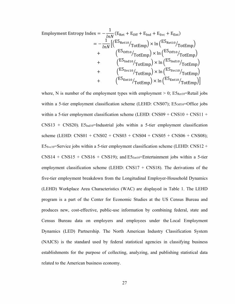
3.1.6. Employment Entropy Index
Employment entropy index is one of the measures that EPA derived to show land use
diversity. A five-tier employment type classification was developed based on the
employment categories of retail, office, industrial, service, and entertainment. It was used
to calculate the employment mix index within each Census Block Group (CBG) by using
the entropy equation applied by Robert Cervero in 1988. For this study, the values were
aggregated in terms of census tract.
27
EmploymentEntropyIndex1
E E E E E
1 E5
TotEmp ln E5TotEmp
E5 TotEmp ln E5TotEmp
E5 TotEmp ln E5TotEmp
E5 TotEmp ln E5TotEmp
E5 TotEmp ln E5TotEmp
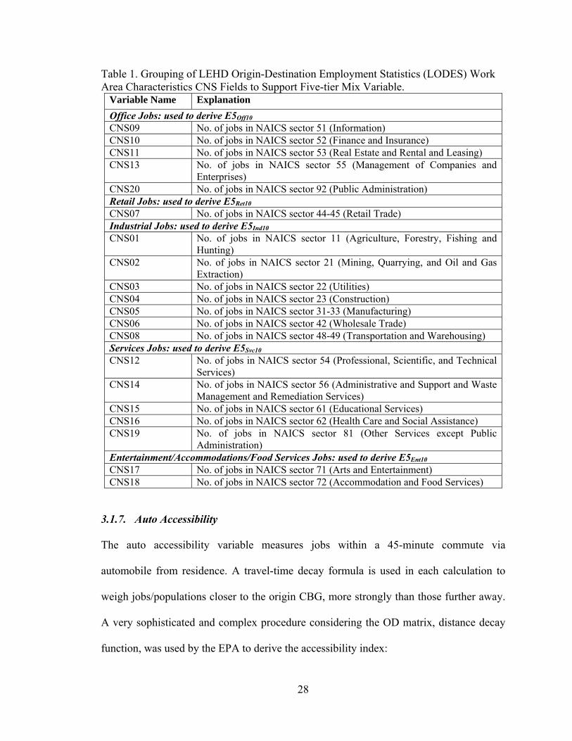
where, N is number of the employment types with employment > 0; E5Ret10=Retail jobs
within a 5-tier employment classification scheme (LEHD: CNS07); E5Off10=Office jobs
within a 5-tier employment classification scheme (LEHD: CNS09 + CNS10 + CNS11 +
CNS13 + CNS20); E5Ind10=Industrial jobs within a 5-tier employment classification
scheme (LEHD: CNS01 + CNS02 + CNS03 + CNS04 + CNS05 + CNS06 + CNS08);
E5Svc10=Service jobs within a 5-tier employment classification scheme (LEHD: CNS12 +
CNS14 + CNS15 + CNS16 + CNS19); andE5Ent10=Entertainment jobs within a 5-tier
employment classification scheme (LEHD: CNS17 + CNS18). The derivations of the
five-tier employment breakdown from the Longitudinal Employer-Household Dynamics
(LEHD) Workplace Area Characteristics (WAC) are displayed in Table 1. The LEHD
program is a part of the Center for Economic Studies at the US Census Bureau and
produces new, cost-effective, public-use information by combining federal, state and
Census Bureau data on employers and employees under the Local Employment
Dynamics (LED) Partnership. The North American Industry Classification System
(NAICS) is the standard used by federal statistical agencies in classifying business
establishments for the purpose of collecting, analyzing, and publishing statistical data
related to the American business economy.
28
Table 1. Grouping of LEHD Origin-Destination Employment Statistics (LODES) Work Area Characteristics CNS Fields to Support Five-tier Mix Variable.
Variable Name Explanation
Office Jobs: used to derive E5Off10 CNS09 No. of jobs in NAICS sector 51 (Information) CNS10 No. of jobs in NAICS sector 52 (Finance and Insurance) CNS11 No. of jobs in NAICS sector 53 (Real Estate and Rental and Leasing) CNS13 No. of jobs in NAICS sector 55 (Management of Companies and
Enterprises) CNS20 No. of jobs in NAICS sector 92 (Public Administration) Retail Jobs: used to derive E5Ret10 CNS07 No. of jobs in NAICS sector 44-45 (Retail Trade) Industrial Jobs: used to derive E5Ind10 CNS01 No. of jobs in NAICS sector 11 (Agriculture, Forestry, Fishing and
Hunting) CNS02 No. of jobs in NAICS sector 21 (Mining, Quarrying, and Oil and Gas
Extraction) CNS03 No. of jobs in NAICS sector 22 (Utilities) CNS04 No. of jobs in NAICS sector 23 (Construction) CNS05 No. of jobs in NAICS sector 31-33 (Manufacturing) CNS06 No. of jobs in NAICS sector 42 (Wholesale Trade) CNS08 No. of jobs in NAICS sector 48-49 (Transportation and Warehousing) Services Jobs: used to derive E5Svc10 CNS12 No. of jobs in NAICS sector 54 (Professional, Scientific, and Technical
Services) CNS14 No. of jobs in NAICS sector 56 (Administrative and Support and Waste
Management and Remediation Services) CNS15 No. of jobs in NAICS sector 61 (Educational Services) CNS16 No. of jobs in NAICS sector 62 (Health Care and Social Assistance) CNS19 No. of jobs in NAICS sector 81 (Other Services except Public
Administration) Entertainment/Accommodations/Food Services Jobs: used to derive E5Ent10 CNS17 No. of jobs in NAICS sector 71 (Arts and Entertainment) CNS18 No. of jobs in NAICS sector 72 (Accommodation and Food Services)
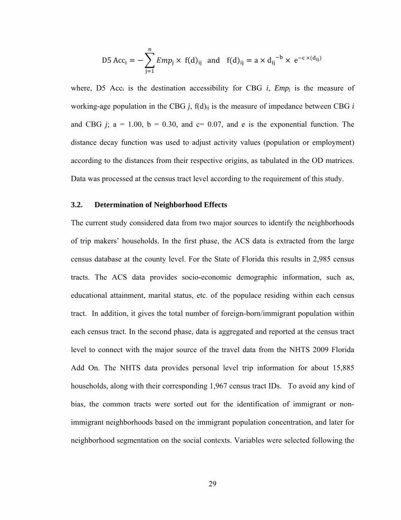
3.1.7. Auto Accessibility
The auto accessibility variable measures jobs within a 45-minute commute via
automobile from residence. A travel-time decay formula is used in each calculation to
weigh jobs/populations closer to the origin CBG, more strongly than those further away.
A very sophisticated and complex procedure considering the OD matrix, distance decay
function, was used by the EPA to derive the accessibility index:
29
D5Acc f d andf d a d e
where, D5 Acci is the destination accessibility for CBG i, Empj is the measure of
working-age population in the CBG j, f(d)ij is the measure of impedance between CBG i
and CBG j; a = 1.00, b = 0.30, and c= 0.07, and e is the exponential function. The
distance decay function was used to adjust activity values (population or employment)
according to the distances from their respective origins, as tabulated in the OD matrices.
Data was processed at the census tract level according to the requirement of this study.
3.2. Determination of Neighborhood Effects
The current study considered data from two major sources to identify the neighborhoods
of trip makers’ households. In the first phase, the ACS data is extracted from the large
census database at the county level. For the State of Florida this results in 2,985 census
tracts. The ACS data provides socio-economic demographic information, such as,
educational attainment, marital status, etc. of the populace residing within each census
tract. In addition, it gives the total number of foreign-born/immigrant population within
each census tract. In the second phase, data is aggregated and reported at the census tract
level to connect with the major source of the travel data from the NHTS 2009 Florida
Add On. The NHTS data provides personal level trip information for about 15,885
households, along with their corresponding 1,967 census tract IDs. To avoid any kind of
bias, the common tracts were sorted out for the identification of immigrant or non-
immigrant neighborhoods based on the immigrant population concentration, and later for
neighborhood segmentation on the social contexts. Variables were selected following the
30
literature on neighborhood definitions in order to reflect the very basic social
background. The unit of data for each variable is processed in percentage against each
tract. After proper cleaning, a total of 1,517 common tract IDs remain for further
analyses. Based on established literature, the census tract level data is used as the base for
segmenting neighborhoods due to its full coverage, cost effectiveness, and convenience
[40].
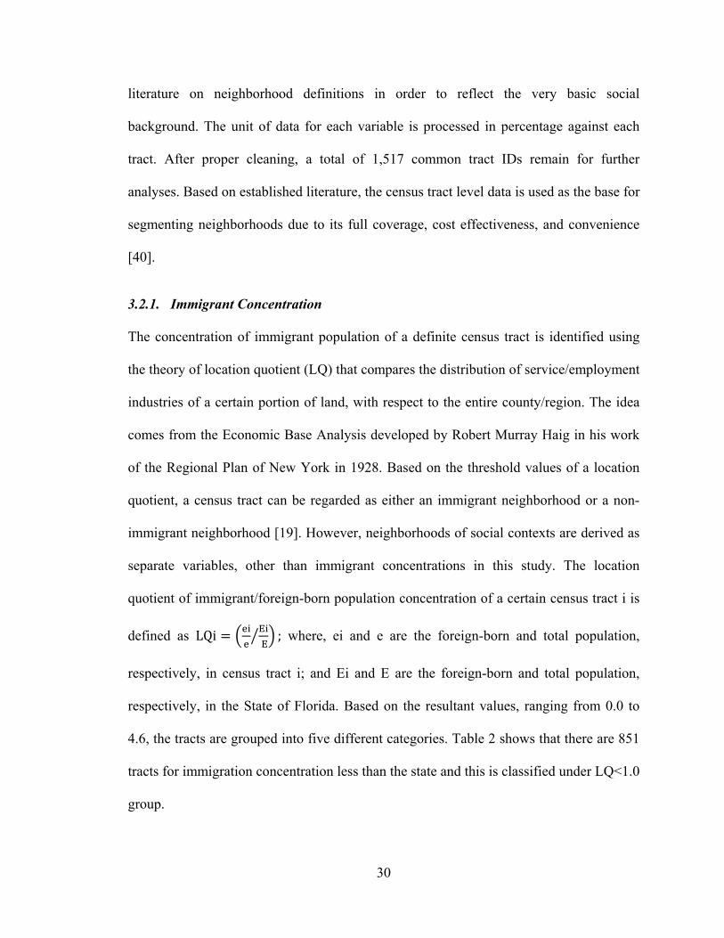
3.2.1. Immigrant Concentration
The concentration of immigrant population of a definite census tract is identified using
the theory of location quotient (LQ) that compares the distribution of service/employment
industries of a certain portion of land, with respect to the entire county/region. The idea
comes from the Economic Base Analysis developed by Robert Murray Haig in his work
of the Regional Plan of New York in 1928. Based on the threshold values of a location
quotient, a census tract can be regarded as either an immigrant neighborhood or a non-
immigrant neighborhood [19]. However, neighborhoods of social contexts are derived as
separate variables, other than immigrant concentrations in this study. The location
quotient of immigrant/foreign-born population concentration of a certain census tract i is
defined as LQi
; where, ei and e are the foreign-born and total population,
respectively, in census tract i; and Ei and E are the foreign-born and total population,
respectively, in the State of Florida. Based on the resultant values, ranging from 0.0 to
4.6, the tracts are grouped into five different categories. Table 2 shows that there are 851
tracts for immigration concentration less than the state and this is classified under LQ<1.0
group.

31
Table 2. Tracts Based on Location Quotient Value of Immigrant Concentration. LQ Value Immigrant Concentration Level of Tracts Number of Tracts LQ <1.0 Less than the state 851 LQ =1.0 Equal to the state 71
1.0< LQ ≤ 2.0 Up to two times the state 434 2.0< LQ ≤ 3.0 Up to three times the state 125 3.0< LQ≤ 4.6 Up to four times or more than the state 45
3.2.2. Neighborhood Typologies
The selection of the variables reflects a critical thought process inspired by established
literature. The first major idea comes from traditional urban sociology that considers
Economic Status, Family Structure and Age Distribution as fundamental neighborhood
characteristics that describe the neighborhood context [59]. The existence of versatile
dimensions makes the settlements different from each other. The second basic idea
reveals that it can be either structural (e.g., economic differentiation) or individual (e.g.,
population traits) [33]. However, this social inequality in terms of socio-economic or
racial segregation between different neighborhoods is significant [60]. Though in
common practice, neighborhood effects are shown through income level or adult groups’
engagement in different jobs, inclusion of individual and family characteristics has also
been suggested in previous studies [41].
The variables include Percentage of Population with less than High School
Degree, Percentage of Population with More than College Degree, Percentage of less
than $25,000/year family income, Percentage of more than or equal to $50,000/year
family income, Families with Dependent Children of Less than or Equal to 18 years,
Percentages of divorced/ separated/widowed people, Percentages of single living people
with no families, Percentages of Employed people. The employment variable was loaded
as a separate factor and resulted in a biased dimension reduction. This may be due to its
32
overlapping with the income variables. Therefore, the Percentages of Employed People
variable was omitted from further analysis. In contrast, the age structure has not been
considered separately because the age issue has already been integrated into the family
structure as Families with Dependent Children of Less than or Equal to 18 years.
Moreover, the inclusion of the variables about marital status gives some indication about
the minimum age of the population. Even though the marriageable age varies from state
to state in the US, the minimum age of marriage in Florida is 16 years (with parental
consent) and legal normal age is 18 years old. In terms of education, the educational
attainment data was used to reflect the context rather than the educational enrollment,
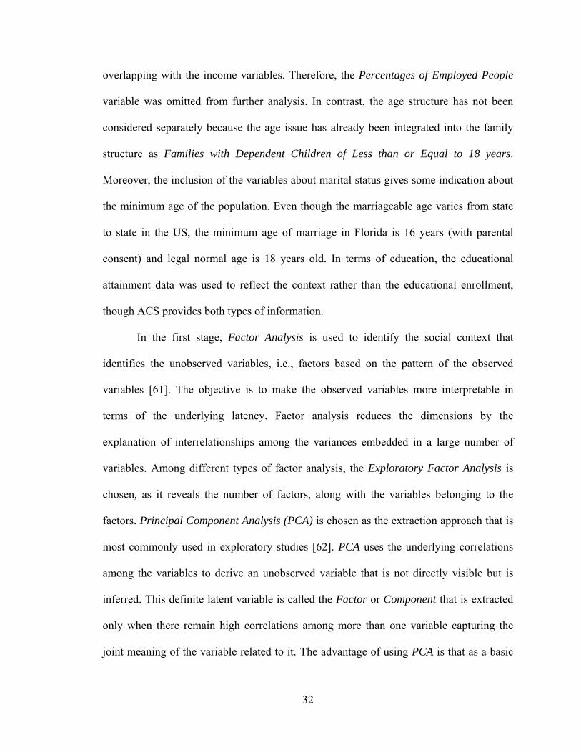
though ACS provides both types of information.
In the first stage, Factor Analysis is used to identify the social context that
identifies the unobserved variables, i.e., factors based on the pattern of the observed
variables [61]. The objective is to make the observed variables more interpretable in
terms of the underlying latency. Factor analysis reduces the dimensions by the
explanation of interrelationships among the variances embedded in a large number of
variables. Among different types of factor analysis, the Exploratory Factor Analysis is
chosen, as it reveals the number of factors, along with the variables belonging to the
factors. Principal Component Analysis (PCA) is chosen as the extraction approach that is
most commonly used in exploratory studies [62]. PCA uses the underlying correlations
among the variables to derive an unobserved variable that is not directly visible but is
inferred. This definite latent variable is called the Factor or Component that is extracted
only when there remain high correlations among more than one variable capturing the
joint meaning of the variable related to it. The advantage of using PCA is that as a basic
33
software feature, SPSS automatically standardizes the values of the new derived variables
[61]. An Orthogonal Varimax Rotation maximized the dispersion of loadings within
factors and enhanced the interpretation. Therefore, there was no need to use the Oblique
Rotation Method. The reliability of the factor extraction is indicated by the Eigenvalues
and the factor Communalities. The Eigenvalue represents the percentage of variance
explained by the extracted factors; whereas the factor Communalities shows the
percentage of variance that can be reproduced through the factor extraction [61]. In this
case, two potential factors are decided on by the significant jump in the slope of the Scree
Plot, which exceeded the Eigenvalue of 1. These two factor scores were derived by the
Regression method against each census tract, and it was the ultimate result of this step.
Factor scores are the linear combination of the observed variables with the factors that
represent the values of the factors [39]. The measurement property, i.e., standardized
values of factor scores make the magnitude of relative importance comparable to one
another. These standardized factor scores are used as input in the next step for clustering
the census tracts into different social groups.
Cluster analysis deals with similar cases of heterogeneous samples and classifies
them into homogenous characteristics based on their distinctive characteristics [63]. This
is one of the most convenient methods used to identify the grouping among objects. The
objects belonging to a specific cluster share similar characteristics but are different from
objects belonging to other clusters [64]. Though the orthogonal nature minimized the
potential bias, it was necessary to remove the outliers, i.e., the extreme cases, to avoid
biasness in the cluster solution [39]. The Q-Q plot of the factor scores (Figure 1) suggests
that the data is normally distributed. Therefore, factor values that exceeded three standard

34
deviations above or below the mean of the factor scores were considered outliers [39] and
subsequently removed from the dataset before the execution of cluster analysis.
Figure 1. Q-Q Plot for (a) Factor 1 and (b) Factor 2 Scores.
The K-means partitioning method was used for the final segmentation. This
nonhierarchical method requires the specification of the expected number of cluster
solutions. If the number of chosen clusters is less or more than the actual number then
the results show error [65]. A two-stage cross validation method was followed for the
determination of actual cluster numbers [66, 67]. Chow, and Li and Chuang
recommended this method to provide confidence of stability after the successful
implementation [39, 40]. The method is initiated with the random division of the entire
dataset into two samples, test sample, and validation sample. Then the test sample is
subjected to Hierarchical Cluster Analysis with Squared Euclidean Distance to get an
initial idea of the potential range of cluster solutions in the data. In this case, Ward’s
method is used, which is a Hierarchical Clustering Algorithm based on Ward’s Minimum
Variance method [64]. The algorithm is designed to minimize the average Squared
Euclidean distance [39, 68]. Finally, the test sample is subjected to the K-means
-4 -2 0 2 4 6-4
-2
0
2
4
E
xpec
ted
No
rmal
Val
ue
Observed Value
Expected Value Reference Line
(a) Factor 1
-4 -2 0 2 4-4
-2
0
2
4
(b) Factor 2
Exp
ecte
d N
orm
al V
alu
e
Observed Value
Expected Value Reference Line

35
Clustering method for each potential set of cluster numbers to obtain the initial centroid
for each cluster.
In the next step, the K-means method is applied twice on the validation sample;
first by specifying the centroids obtained from the test sample, and then without using the
centroids. The classification results identified by the two procedures for a given number
of clusters are then compared in terms of Kappa-statistics. This is a chance-corrected
coefficient of agreement where a high coefficient suggests a high agreement between the
two datasets [69]. The exact numbers of clusters that reveal the highest coefficient in the
Kappa statistics are chosen and applied to the K-means partitioning method on the entire
dataset. As a result of this classification, each census tract is assigned with a specific
cluster number. Consequently, in the mode choice model, each trip maker’s household
becomes assigned with the same cluster number of its accommodating census tract. This
method of cluster analysis, followed by the factor analysis, makes the understanding and
the classification patterns clear and stable.
The rule of thumb of factor analysis is that it requires at least five variables and
ten samples to identify latent components [61]. The dataset containing seven variables of
1,517 cases fulfills the basic requirement and confirms the validity. However, the
implementation of PCA has a pre-requisite suitability test that deals with correlation
among the variables. The test is normally identified by two measures. According to the
first measure, the values of the correlation matrix exceeding the threshold of absolute
0.30 indicate that the conduction of PCA is supposed to be useful. The Anti-Image is
another measure of determination used to understand whether the items are sufficiently
correlated. It describes an item’s portion that is independent of another item in the
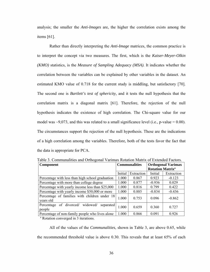
36
analysis; the smaller the Anti-Images are, the higher the correlation exists among the
items [61].
Rather than directly interpreting the Anti-Image matrices, the common practice is
to interpret the concept via two measures. The first, which is the Kaiser-Meyer-Olkin
(KMO) statistics, is the Measure of Sampling Adequacy (MSA). It indicates whether the
correlation between the variables can be explained by other variables in the dataset. An
estimated KMO value of 0.718 for the current study is middling, but satisfactory [70].
The second one is Bartlett’s test of sphericity, and it tests the null hypothesis that the
correlation matrix is a diagonal matrix [61]. Therefore, the rejection of the null
hypothesis indicates the existence of high correlation. The Chi-square value for our
model was ~9,073, and this was related to a small significance level (i.e., p-value = 0.00).
The circumstances support the rejection of the null hypothesis. These are the indications
of a high correlation among the variables. Therefore, both of the tests favor the fact that
the data is appropriate for PCA.
Table 3. Communalities and Orthogonal Varimax Rotation Matrix of Extended Factors. Component Communalities Orthogonal Varimax
Rotation Matrixa
Initial Extraction Initial ExtractionPercentage with less than high school graduation 1.000 0.867 0.923 -0.123Percentage with more than college degree 1.000 0.877 -0.936 0.029Percentage with yearly income less than $25,000 1.000 0.816 0.799 0.422Percentage with yearly income $50,000 or more 1.000 0.885 -0.834 -0.436Percentage of families with children under 18 years old 1.000 0.753 0.096 -0.862
Percentage of divorced/ widowed/ separated people 1.000 0.659 0.360 0.727
Percentage of non-family people who lives alone 1.000 0.866 0.091 0.926a Rotation converged in 3 iterations.
All of the values of the Communalities, shown in Table 3, are above 0.65, while
the recommended threshold value is above 0.30. This reveals that at least 65% of each
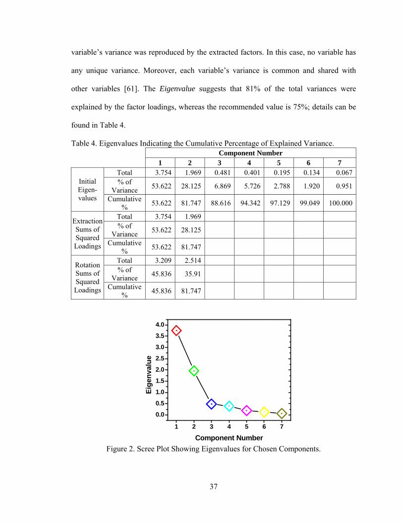
37
variable’s variance was reproduced by the extracted factors. In this case, no variable has
any unique variance. Moreover, each variable’s variance is common and shared with
other variables [61]. The Eigenvalue suggests that 81% of the total variances were
explained by the factor loadings, whereas the recommended value is 75%; details can be
found in Table 4.
Table 4. Eigenvalues Indicating the Cumulative Percentage of Explained Variance.
Component Number
1 2 3 4 5 6 7
Initial Eigen-values
Total 3.754 1.969 0.481 0.401 0.195 0.134 0.067% of
Variance 53.622 28.125 6.869 5.726 2.788 1.920 0.951
Cumulative %
53.622 81.747 88.616 94.342 97.129 99.049 100.000
Extraction Sums of Squared Loadings
Total 3.754 1.969 % of
Variance 53.622 28.125
Cumulative %
53.622 81.747
Rotation Sums of Squared Loadings
Total 3.209 2.514 % of
Variance 45.836 35.91
Cumulative %
45.836 81.747
Figure 2. Scree Plot Showing Eigenvalues for Chosen Components.
1 2 3 4 5 6 7
0.0
0.5
1.0
1.5
2.0
2.5
3.0
3.5
4.0
Eig
enva
lue
Component Number
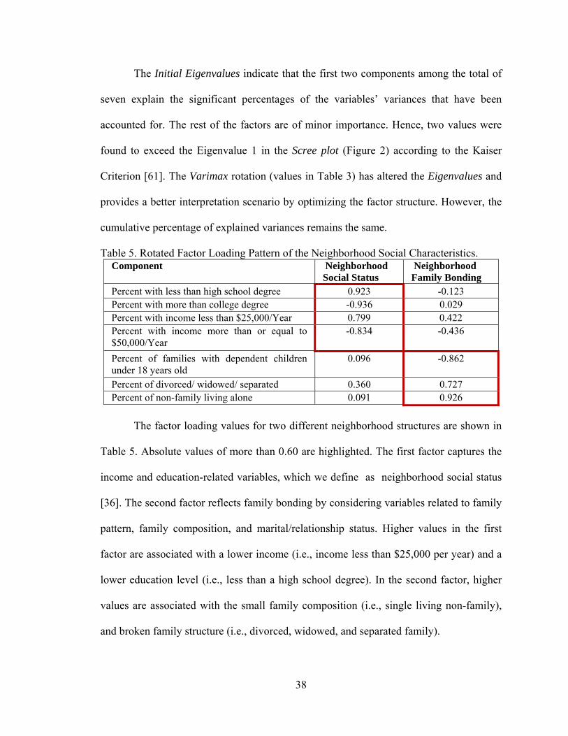
38
The Initial Eigenvalues indicate that the first two components among the total of
seven explain the significant percentages of the variables’ variances that have been
accounted for. The rest of the factors are of minor importance. Hence, two values were
found to exceed the Eigenvalue 1 in the Scree plot (Figure 2) according to the Kaiser
Criterion [61]. The Varimax rotation (values in Table 3) has altered the Eigenvalues and
provides a better interpretation scenario by optimizing the factor structure. However, the
cumulative percentage of explained variances remains the same.
Table 5. Rotated Factor Loading Pattern of the Neighborhood Social Characteristics. Component Neighborhood
Social Status Neighborhood Family Bonding
Percent with less than high school degree 0.923 -0.123 Percent with more than college degree -0.936 0.029 Percent with income less than $25,000/Year 0.799 0.422 Percent with income more than or equal to $50,000/Year
-0.834 -0.436
Percent of families with dependent children under 18 years old
0.096 -0.862
Percent of divorced/ widowed/ separated 0.360 0.727 Percent of non-family living alone 0.091 0.926
The factor loading values for two different neighborhood structures are shown in
Table 5. Absolute values of more than 0.60 are highlighted. The first factor captures the
income and education-related variables, which we define as neighborhood social status
[36]. The second factor reflects family bonding by considering variables related to family
pattern, family composition, and marital/relationship status. Higher values in the first
factor are associated with a lower income (i.e., income less than $25,000 per year) and a
lower education level (i.e., less than a high school degree). In the second factor, higher
values are associated with the small family composition (i.e., single living non-family),
and broken family structure (i.e., divorced, widowed, and separated family).
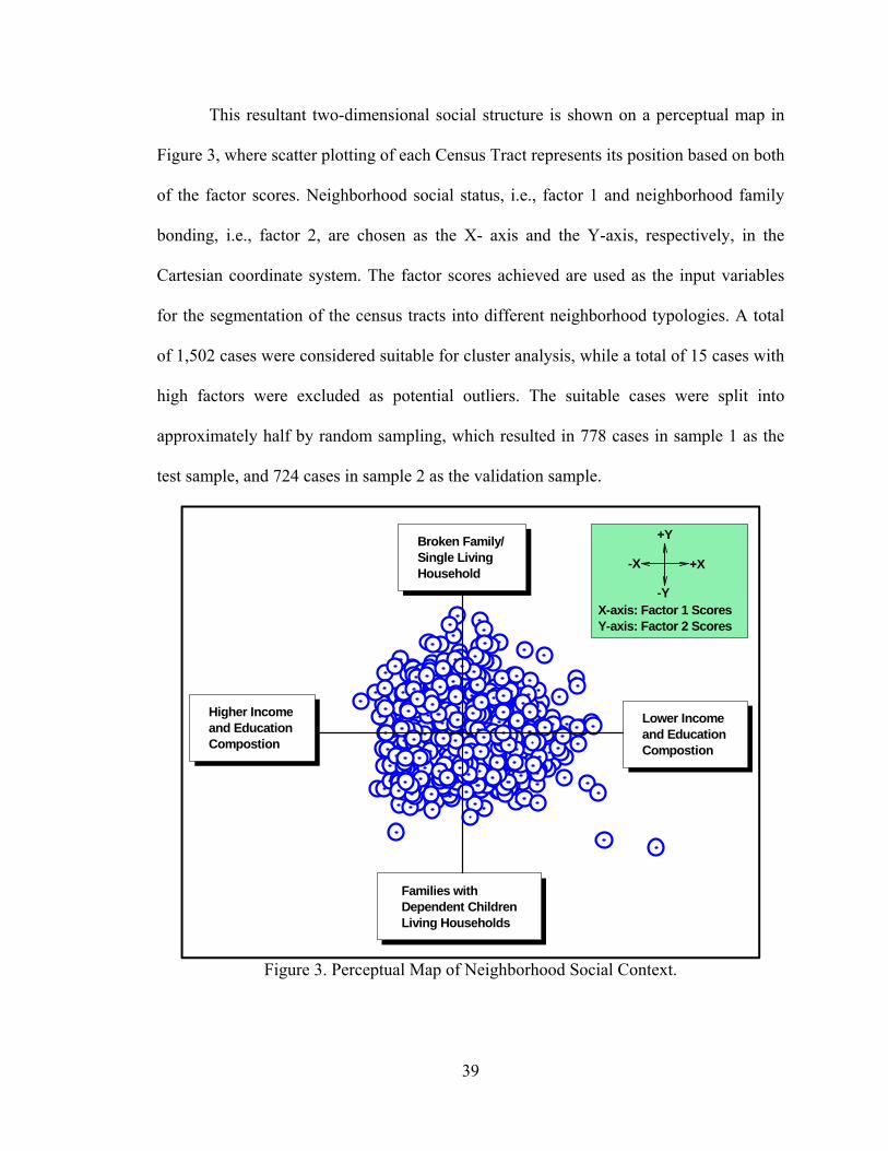
39
This resultant two-dimensional social structure is shown on a perceptual map in
Figure 3, where scatter plotting of each Census Tract represents its position based on both
of the factor scores. Neighborhood social status, i.e., factor 1 and neighborhood family
bonding, i.e., factor 2, are chosen as the X- axis and the Y-axis, respectively, in the
Cartesian coordinate system. The factor scores achieved are used as the input variables
for the segmentation of the census tracts into different neighborhood typologies. A total
of 1,502 cases were considered suitable for cluster analysis, while a total of 15 cases with
high factors were excluded as potential outliers. The suitable cases were split into
approximately half by random sampling, which resulted in 778 cases in sample 1 as the
test sample, and 724 cases in sample 2 as the validation sample.
Figure 3. Perceptual Map of Neighborhood Social Context.
-Y
+Y
-X +X
Lower Income and Education Compostion
Broken Family/ Single Living Household
Families withDependent ChildrenLiving Households
Higher Income and Education Compostion
X-axis: Factor 1 ScoresY-axis: Factor 2 Scores

40
Application of the Ward’s method of Hierarchical Clustering on the test sample
suggested two to four potential clusters from the Dendrogram tree. The initial centroids
are generated using the K-means clustering method for each cluster and consequently
applied on the validation sample. The validation sample is subjected to K-means
clustering again and this time without specifying the initial centroids. The cluster
segmentation results are compared with the Kappa statistics of agreement, and the
coefficients are achieved as 0.373, 0.983 and 0.183 for two, three, and four cluster
numbers, respectively. Therefore, the three-cluster segmentation appears to be optimal.
Then the K-means cluster analysis is applied over the entire dataset with specification of
three clusters. The three typologies of the neighborhood conditions are listed in Table 6.
The values represent the cluster means of the factor scores and the number of cases
within each type.
Table 6. Distribution of Census Tracts under Two Neighborhood Factors.
Factor Neighborhood Typologies
Type 1 (N=532)
Type 2 (N=483)
Type 3 (N=487)
Outliers (N=15)
1: Neighborhood Social Status Structure a 0.95 -0.82 -0.3 2.01 2: Neighborhood Family Bonding Structure b -0.27 -0.75 1.02 0.67 a Higher scores represent lower level of educational attainment and household income. b High scores represent more broken family/ single living households than family living with dependent children in the household.
About 532 tracts are segmented as Type 1 of Neighborhood. In this type, the
majority of the population has a lower income level and educational attainment, and a
higher share in families with dependent children. Therefore, this type of neighborhood is
characterized as Low Social Status along with High Family Bonding and is found as the
highest in shares. The second typology, i.e., Type 2, has lower scores in both factors,
which represents the fact that this neighborhood type is characterized by High Social

41
Status along with High Family Bonding. About 483 tracts are grouped in this category.
The third one is majored with a higher percentage of divorced/widowed/separated
population and single living households, as well as a higher educational attainment and
income combination. Therefore, this type indicates the High Social Status with Low
Family Bonding, which captures about 487 census tracts within itself. The fourth
combination consists of extreme values in both of the factors. Therefore, the
neighborhood type holds the Extremely Low Social Status with Low Family Bonding. The
15 outlier values of extreme cases are segmented in this category.
Figure 4. Distribution of Neighborhood Typologies throughout the Florida State.
42
The dispersion of the neighborhood typologies is shown in the map of Florida in
Figure 4. The colored region includes type 1 to 3, and outliers of cluster analysis. These
represent the census tracts of trip makers' household locations, provided by NHTS tract
data. The white region indicates those census tracts in Florida where there is no existence
of trip makers’ households. These census tracts are not included in the NHTS tract data
set and are also excluded for neighborhood segmentation to avoid bias since factor and
cluster analyses works on the variables’ variances.
3.3. Behavioral Assimilation Analysis
Studies on California immigrants suggest that the travel behavior of immigrants leans
towards the US-born Americans [14]. However, it does not answer the question of what
the paradigm is in the case of a uniquely demographic Florida region. To address this
question, our goal is to testify whether or not adding the arrival/migration period in the
mode choice model as an exploratory variable is required. A household is considered to
be “immigrant” if at least one foreign-born member exists there. It is important to note
that a household is not considered to be US-born even if there is at least one US-born
member. This reasoning comes from the fact that the immigrants’ children are Americans
by birth, however the household’s characteristics, travel pattern, etc., cannot be profiled
through the younger family members; rather, by the adults. In addition, the foreign-born
households are divided into five gradual categories based on their arrival year in the US.
In this case, the oldest year reported by any of the household members is taken into
consideration. Immigrants’ socio-economic and demographic characteristics, e.g., race;
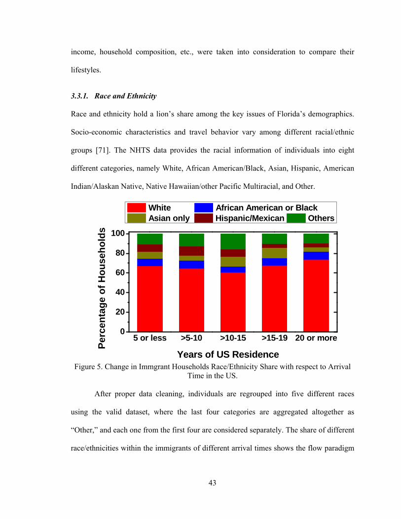
43
income, household composition, etc., were taken into consideration to compare their
lifestyles.
3.3.1. Race and Ethnicity
Race and ethnicity hold a lion’s share among the key issues of Florida’s demographics.
Socio-economic characteristics and travel behavior vary among different racial/ethnic
groups [71]. The NHTS data provides the racial information of individuals into eight
different categories, namely White, African American/Black, Asian, Hispanic, American
Indian/Alaskan Native, Native Hawaiian/other Pacific Multiracial, and Other.
Figure 5. Change in Immgrant Households Race/Ethnicity Share with respect to Arrival
Time in the US.
After proper data cleaning, individuals are regrouped into five different races
using the valid dataset, where the last four categories are aggregated altogether as
“Other,” and each one from the first four are considered separately. The share of different
race/ethnicities within the immigrants of different arrival times shows the flow paradigm
5 or less >5-10 >10-15 >15-19 20 or more0
20
40
60
80
100
Per
cen
tag
e o
f H
ou
seh
old
s
Years of US Residence
White African American or Black Asian only Hispanic/Mexican Others
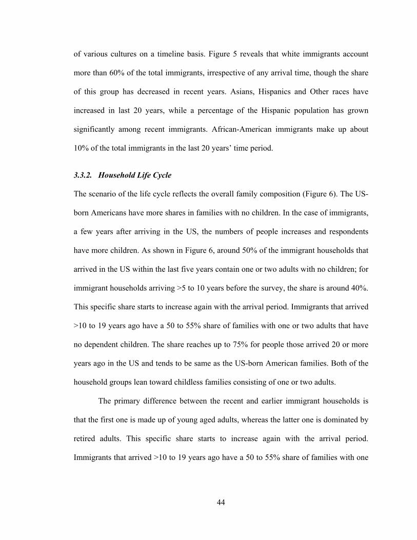
44
of various cultures on a timeline basis. Figure 5 reveals that white immigrants account
more than 60% of the total immigrants, irrespective of any arrival time, though the share
of this group has decreased in recent years. Asians, Hispanics and Other races have
increased in last 20 years, while a percentage of the Hispanic population has grown
significantly among recent immigrants. African-American immigrants make up about
10% of the total immigrants in the last 20 years’ time period.
3.3.2. Household Life Cycle
The scenario of the life cycle reflects the overall family composition (Figure 6). The US-
born Americans have more shares in families with no children. In the case of immigrants,
a few years after arriving in the US, the numbers of people increases and respondents
have more children. As shown in Figure 6, around 50% of the immigrant households that
arrived in the US within the last five years contain one or two adults with no children; for
immigrant households arriving >5 to 10 years before the survey, the share is around 40%.
This specific share starts to increase again with the arrival period. Immigrants that arrived
>10 to 19 years ago have a 50 to 55% share of families with one or two adults that have
no dependent children. The share reaches up to 75% for people those arrived 20 or more
years ago in the US and tends to be same as the US-born American families. Both of the
household groups lean toward childless families consisting of one or two adults.
The primary difference between the recent and earlier immigrant households is
that the first one is made up of young aged adults, whereas the latter one is dominated by
retired adults. This specific share starts to increase again with the arrival period.
Immigrants that arrived >10 to 19 years ago have a 50 to 55% share of families with one
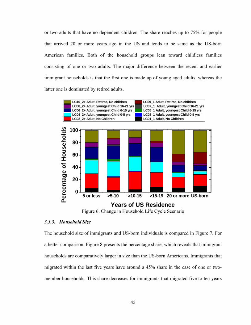
45
or two adults that have no dependent children. The share reaches up to 75% for people
that arrived 20 or more years ago in the US and tends to be same as the US-born
American families. Both of the household groups lean toward childless families
consisting of one or two adults. The major difference between the recent and earlier
immigrant households is that the first one is made up of young aged adults, whereas the
latter one is dominated by retired adults.
Figure 6. Change in Household Life Cycle Scenario
3.3.3. Household Size
The household size of immigrants and US-born individuals is compared in Figure 7. For
a better comparison, Figure 8 presents the percentage share, which reveals that immigrant
households are comparatively larger in size than the US-born Americans. Immigrants that
migrated within the last five years have around a 45% share in the case of one or two-
member households. This share decreases for immigrants that migrated five to ten years
5 or less >5-10 >10-15 >15-19 20 or more US-born0
20
40
60
80
100
LC10_2+ Adult, Retired, No children LC09_1 Adult, Retired, No children LC08_2+ Adult, youngest Child 16-21 yrs LC07_1 Adult, youngest Child 16-21 yrs LC06_2+ Adult, youngest Child 6-15 yrs LC05_1 Adult, youngest Child 6-15 yrs LC04_2+ Adult, youngest Child 0-5 yrs LC03_1 Adult, youngest Child 0-5 yrs LC02_2+ Adult, No Children LC01_1 Adult, No Children
Per
cen
tag
e o
f H
ou
seh
old
s
Years of US Residence
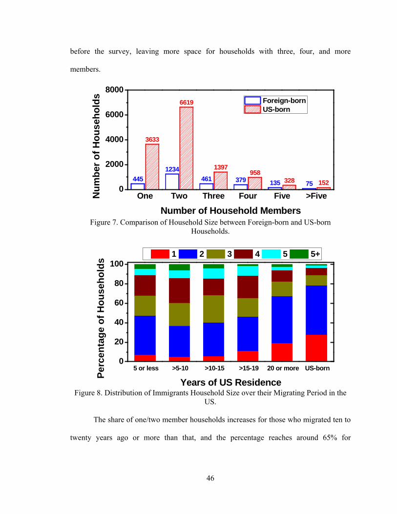
46
before the survey, leaving more space for households with three, four, and more
members.
Figure 7. Comparison of Household Size between Foreign-born and US-born
Households.
Figure 8. Distribution of Immigrants Household Size over their Migrating Period in the
US.
The share of one/two member households increases for those who migrated ten to
twenty years ago or more than that, and the percentage reaches around 65% for
445
1234
461 379 135 75
3633
6619
1397958
328 152
One Two Three Four Five >Five0
2000
4000
6000
8000N
um
ber
of
Ho
use
ho
lds
Number of Household Members
Foreign-born US-born
5 or less >5-10 >10-15 >15-19 20 or more US-born0
20
40
60
80
100 1 2 3 4 5 5+
Per
cen
tag
e o
f H
ou
seh
old
s
Years of US Residence
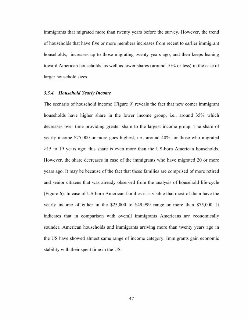
47
immigrants that migrated more than twenty years before the survey. However, the trend
of households that have five or more members increases from recent to earlier immigrant
households, increases up to those migrating twenty years ago, and then keeps leaning
toward American households, as well as lower shares (around 10% or less) in the case of
larger household sizes.
3.3.4. Household Yearly Income
The scenario of household income (Figure 9) reveals the fact that new comer immigrant
households have higher share in the lower income group, i.e., around 35% which
decreases over time providing greater share to the largest income group. The share of
yearly income $75,000 or more goes highest, i.e., around 40% for those who migrated
>15 to 19 years ago; this share is even more than the US-born American households.
However, the share decreases in case of the immigrants who have migrated 20 or more
years ago. It may be because of the fact that these families are comprised of more retired
and senior citizens that was already observed from the analysis of household life-cycle
(Figure 6). In case of US-born American families it is visible that most of them have the
yearly income of either in the $25,000 to $49,999 range or more than $75,000. It
indicates that in comparison with overall immigrants Americans are economically
sounder. American households and immigrants arriving more than twenty years ago in
the US have showed almost same range of income category. Immigrants gain economic
stability with their spent time in the US.
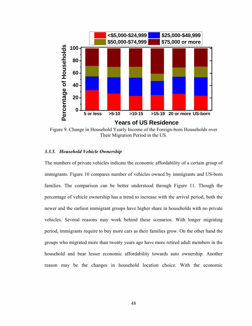
48
Figure 9. Change in Household Yearly Income of the Foreign-born Households over
Their Migration Period in the US.
3.3.5. Household Vehicle Ownership
The numbers of private vehicles indicate the economic affordability of a certain group of
immigrants. Figure 10 compares number of vehicles owned by immigrants and US-born
families. The comparison can be better understood through Figure 11. Though the
percentage of vehicle ownership has a trend to increase with the arrival period, both the
newer and the earliest immigrant groups have higher share in households with no private
vehicles. Several reasons may work behind these scenarios. With longer migrating
period, immigrants require to buy more cars as their families grow. On the other hand the
groups who migrated more than twenty years ago have more retired adult members in the
household and bear lesser economic affordability towards auto ownership. Another
reason may be the changes in household location choice. With the economic
5 or less >5-10 >10-15 >15-19 20 or more US-born0
20
40
60
80
100
Per
cen
tag
e o
f H
ou
seh
old
s
Years of US Residence
<$5,000-$24,999 $25,000-$49,999 $50,000-$74,999 $75,000 or more
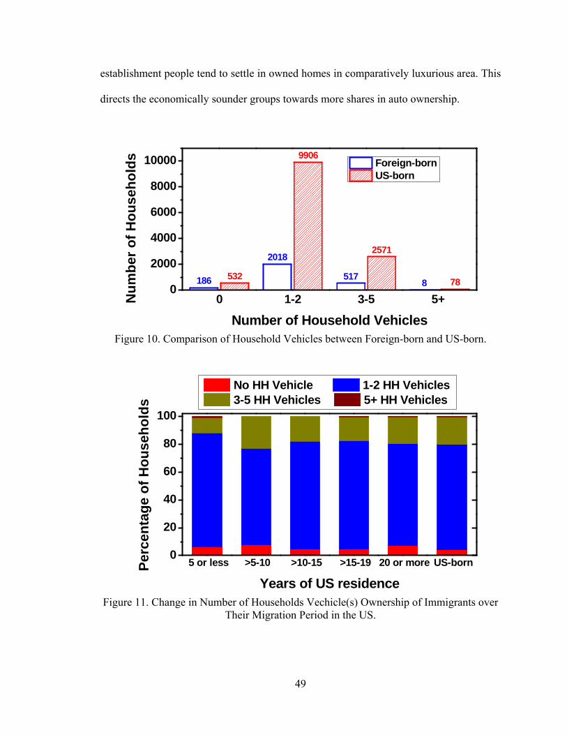
49
establishment people tend to settle in owned homes in comparatively luxurious area. This
directs the economically sounder groups towards more shares in auto ownership.
Figure 10. Comparison of Household Vehicles between Foreign-born and US-born.
Figure 11. Change in Number of Households Vechicle(s) Ownership of Immigrants over
Their Migration Period in the US.
186
2018
5178
532
9906
2571
78
0 1-2 3-5 5+ 0
2000
4000
6000
8000
10000
Nu
mb
er o
f H
ou
seh
old
s
Number of Household Vehicles
Foreign-born US-born
5 or less >5-10 >10-15 >15-19 20 or more US-born0
20
40
60
80
100
Per
cen
tag
e o
f H
ou
seh
old
s
Years of US residence
No HH Vehicle 1-2 HH Vehicles 3-5 HH Vehicles 5+ HH Vehicles
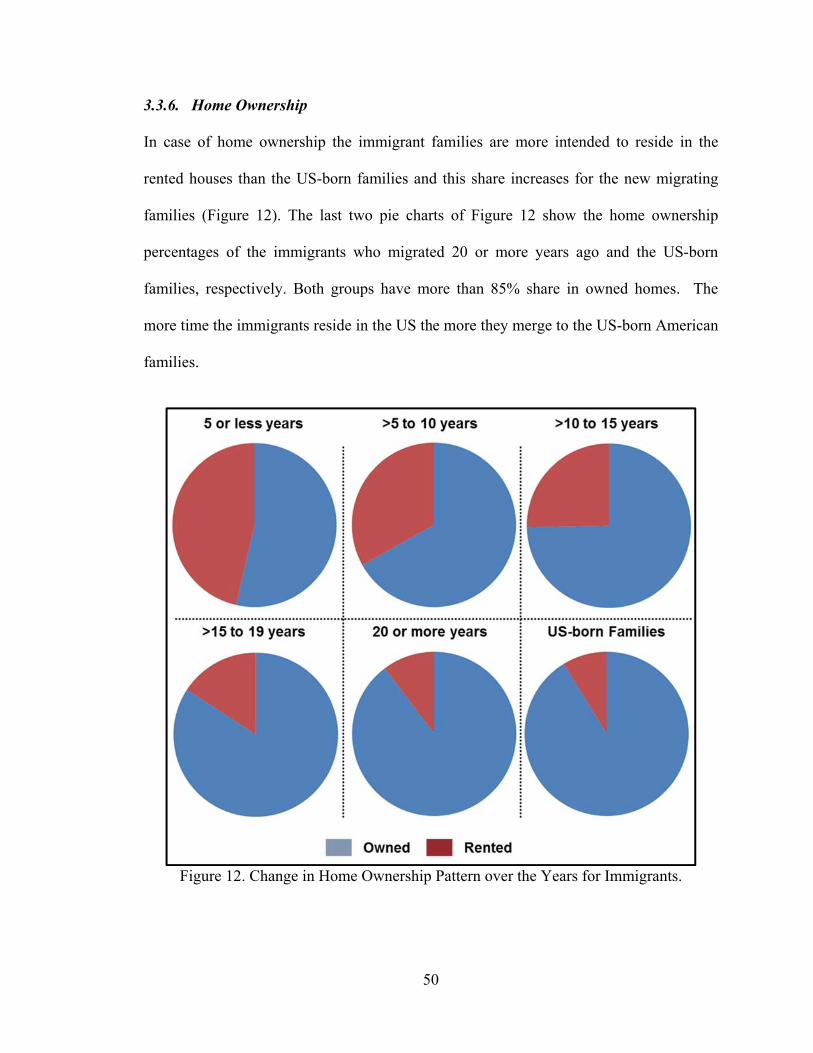
50
3.3.6. Home Ownership
In case of home ownership the immigrant families are more intended to reside in the
rented houses than the US-born families and this share increases for the new migrating
families (Figure 12). The last two pie charts of Figure 12 show the home ownership
percentages of the immigrants who migrated 20 or more years ago and the US-born
families, respectively. Both groups have more than 85% share in owned homes. The
more time the immigrants reside in the US the more they merge to the US-born American
families.
Figure 12. Change in Home Ownership Pattern over the Years for Immigrants.
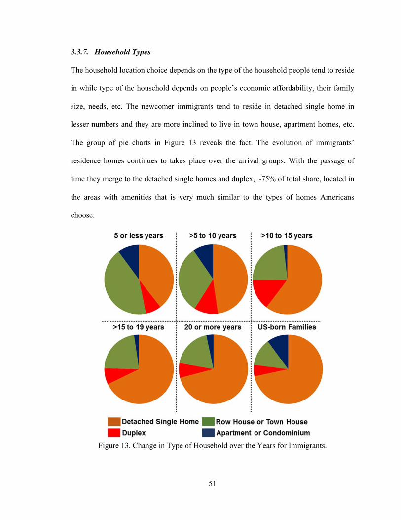
51
3.3.7. Household Types
The household location choice depends on the type of the household people tend to reside
in while type of the household depends on people’s economic affordability, their family
size, needs, etc. The newcomer immigrants tend to reside in detached single home in
lesser numbers and they are more inclined to live in town house, apartment homes, etc.
The group of pie charts in Figure 13 reveals the fact. The evolution of immigrants’
residence homes continues to takes place over the arrival groups. With the passage of
time they merge to the detached single homes and duplex, ~75% of total share, located in
the areas with amenities that is very much similar to the types of homes Americans
choose.
Figure 13. Change in Type of Household over the Years for Immigrants.
52
3.4. Summary
This chapter describes how to incorporate available data to determine the land use
variables needed for the Florida census tract. In addition, four types of neighborhood
typologies were derived from fundamental neighborhood characteristics (i.e., economic
status, family structure, and age distribution) by conducting a factor analysis, followed by
a cluster analysis. Moreover, the concentration of immigrant populations was classified
into five groups, with respect to the location quotient values of the Florida census tract. In
the next chapter, the combination of the geographic aspects of neighborhood, such as
land use indices, and neighborhood attributes such as neighborhood typology and
immigrant concentration, will represent the overall neighborhood effects used in the final
model development. Furthermore, the behavioral assimilation analyses provide a general
idea of how immigrants move toward the lifestyle of the US-born individuals as they
spend more time in the US. This information is reflected through their income, household
size, vehicle ownership, and family, social, and demographic characteristics. Immigrants’
changes in lifestyle significantly alter their travel behavior. Therefore, it is important to
integrate the arrival period as a variable in the mode choice model.
53
4. METHODOLOGY
4.1. Hypothesis
The establishment of the conceptual framework is rooted in the literature review and
continues toward the final completion of the model’s development to meet the goals and
objectives of this study. The models are developed based on the following hypotheses.
o Hypothesis 1: The neighborhood effects that impact individuals’ travel behavior
are comprised of something beyond the areas’ density, size, etc. It cannot be
generalized that only living in higher immigrant-populated areas make people
more likely to use alternative modes.
o Hypothesis 2: Immigrants’ change in preference toward the alternative mode
usage is associated with their household life cycle, race, size, and lifestyle
changes, as well as time spent in the US.
4.2. Model Structure
At this stage, Multinomial Logit Models have been developed for work, shopping, social,
recreational, and other (i.e., school, religious, personal business, maintenance, etc.) trip
purposes to examine the influence of the determinant factors such as personal, household,
land use, neighborhood, and immigrant attributes on the choice of travel mode, i.e., drive
alone, carpool, transit, and walk and bike. Significance of immigrant indicators was
examined with or without additional neighborhood and assimilation variables. The model
takes the functional form:
logit P ln P1 P α βX
54
where, P is probability for certain events to occur, [P/(1-P)] is odds ratio (OR), which
indicates the ratio of the probability of the occurrence of that certain event over the
probability of not occurring of that event, and are estimated coefficients using the
maximum likelihood estimation, and X is vector of the corresponding determinant factor.
Incorporating all the attributes considered in the current study, the model takes the
following form:
logit P lnP
1 Pα β PR β HH β LU β LQ β IM β NH
where, Pmode is the probability that a certain mode is chosen, [Pmode/(1-Pmode)] is the odds
ratio (OR) that indicates the ratio of the probability of choosing a certain mode over the
probability of not choosing the mode, ln[Pmode/(1-Pmode)] is the log odds, PR is the vector
of person-level variables that has been proved to be a determinant in mode choice
behavior in previous literature, HH is the vector of household-level determinants of mode
choice, LU is the vector of land use variables, as well as built environment determinants
of mode choice, LQ is the vector of the location quotient of immigrant population
concentration, IM is the vector of immigrant related variables (i.e., foreign-born status
and arrival period in USA), NH is the vector of neighborhood typologies, and
αandβ …. are estimated coefficients using the maximum likelihood estimation.
The modeled choice outcomes include single-occupant vehicle (SOV)
representing drive alone (the base category), carpool or shared ride (i.e., all auto trips
with more than one occupant), public transportation, and walking and biking as the two
non-motorized transport (NMT). Among the personal and household variables, gender,
educational attainment, driver status, household income group, household type, home
55
ownership, household life cycle, etc., are selected as categorical dummy variables;
whereas age, number of household adult members and vehicles, household size, etc., are
chosen as continuous variables. Among the immigrant-related variables, the foreign-born
or immigrant status of a trip maker is used as a dummy variable, whereas the earliest
arrival period reported by any of the household members is considered the categorization
criterion for the foreign-born households and further creation of the dummy variables. In
this context, the presence of one or more foreign-born members is used as the indicator
for considering a household as foreign-born/immigrant household. The derived land use
variables are used as continuous variables; whereas the location quotient of immigrant
concentration and the neighborhood typologies were considered as categorical dummy
variables.
After proper data processing, a total of 53,314 trip records remain for the final
model development. Out of these trips, 7,132, 20,058, 11,753, and 14,371 trips are
classified as work, shopping, social and recreational, and other trips, respectively. The
non-home based trips are not taken into account as they are not assumed to directly
represent the mode choice behavior describing the trip maker’s household location
choice, neighborhood patterns, etc. The initial idea about each of the single variables and
their relationships with the dependent variable was obtained by using the SAS (Statistical
Analysis System) software. However, due to its large data handling constraints, the final
models are developed using the Blerlaire Optimization toolbox for GEv Model
Estimation, commonly known as BIOGEME 1.8 freeware package that is designed for
the development of research in the context of discrete choice models in general.
56
5. RESULTS AND DISCUSSIONS
The multinomial logistic regression models were developed for work, shopping, social,
recreational, and other trips. Attributes of personal, household, immigrant status, land
use, and neighborhood were chosen as independent variables. The initial assessment of
the model was done through the Goodness-of-fit test measures and the statistical test. The
rho-square measure is widely used to describe the goodness-of-fit for the discrete choice
models because of their intuitive formulation [72]. The Rho-square values for work,
shopping, social, recreational, and other trips are reported as 0.719, 0.450, 0.223, and
0.327, respectively. Previous studies on MNL models have shown similar results. Enam
and Choudhury reported a Rho-square value of 0.270 for developed MNL models
considering 15 types of different modes [73]. Saha reported Rho square values of 0.336
and 0.344 for work and education-based trips, respectively [74]. Thereby, both the rho-
square and adjusted rho-square values are satisfactory in the developed models.
Specifically, for work trip model, the value exceeded 0.70, which indicates that the
predicted models are close to perfect. The detailed results of the multinomial logistic
regression model of each trip are shown in Tables 7 through 10. The estimated
coefficients based on the Utility Maximization Theory, along with their t-test and
significance level, elaborate the detailed influence of corresponding variables on the trip
maker’s odds of choosing any of the three alternative modes, i.e., high-occupancy vehicle
(carpooling/ride sharing), public transit, and non-motorized transport (walking/biking)
over single-occupant vehicles (SOV) or driving alone.
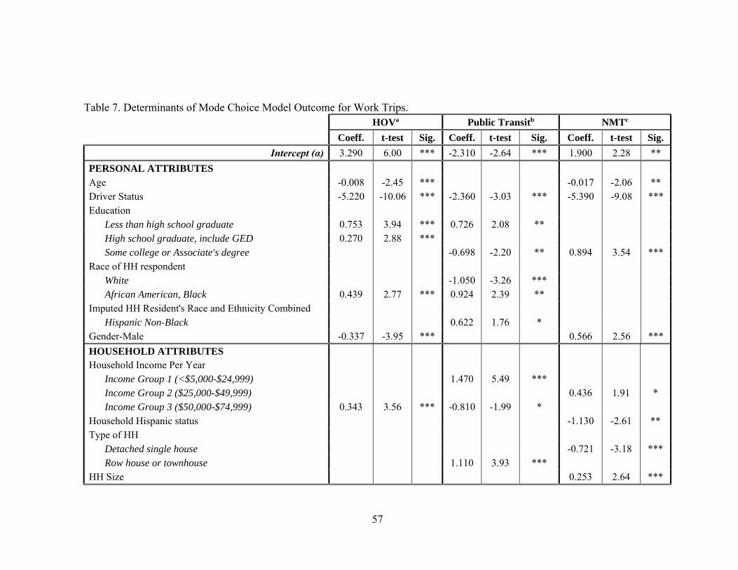
57
Table 7. Determinants of Mode Choice Model Outcome for Work Trips. HOVa Public Transitb NMTc
Coeff. t-test Sig. Coeff. t-test Sig. Coeff. t-test Sig.
Intercept (α) 3.290 6.00 *** -2.310 -2.64 *** 1.900 2.28 **
PERSONAL ATTRIBUTES Age -0.008 -2.45 *** -0.017 -2.06 ** Driver Status -5.220 -10.06 *** -2.360 -3.03 *** -5.390 -9.08 *** Education
Less than high school graduate 0.753 3.94 *** 0.726 2.08 ** High school graduate, include GED 0.270 2.88 *** Some college or Associate's degree -0.698 -2.20 ** 0.894 3.54 ***
Race of HH respondent White -1.050 -3.26 *** African American, Black 0.439 2.77 *** 0.924 2.39 **
Imputed HH Resident's Race and Ethnicity Combined Hispanic Non-Black 0.622 1.76 *
Gender-Male -0.337 -3.95 *** 0.566 2.56 ***
HOUSEHOLD ATTRIBUTES Household Income Per Year
Income Group 1 (<$5,000-$24,999) 1.470 5.49 *** Income Group 2 ($25,000-$49,999) 0.436 1.91 * Income Group 3 ($50,000-$74,999) 0.343 3.56 *** -0.810 -1.99 *
Household Hispanic status -1.130 -2.61 ** Type of HH
Detached single house -0.721 -3.18 *** Row house or townhouse 1.110 3.93 ***
HH Size 0.253 2.64 ***
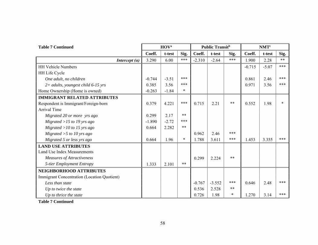
58
Table 7 Continued HOVa Public Transitb NMTc
Coeff. t-test Sig. Coeff. t-test Sig. Coeff. t-test Sig.
Intercept (α) 3.290 6.00 *** -2.310 -2.64 *** 1.900 2.28 **
HH Vehicle Numbers -0.715 -5.07 *** HH Life Cycle
One adult, no children -0.744 -3.51 *** 0.861 2.46 *** 2+ adults, youngest child 6-15 yrs 0.385 3.56 *** 0.971 3.56 ***
Home Ownership (Home is owned) -0.263 -1.84 *
IMMIGRANT RELATED ATTRIBUTES Respondent is Immigrant/Foreign-born 0.379 4.221 *** 0.715 2.21 ** 0.552 1.98 * Arrival Time
Migrated 20 or more yrs ago 0.299 2.17 ** Migrated >15 to 19 yrs ago -1.890 -2.72 *** Migrated >10 to 15 yrs ago 0.664 2.282 ** Migrated >5 to 10 yrs ago 0.962 2.46 *** Migrated 5 or less yrs ago 0.664 1.96 * 1.788 3.611 *** 1.453 3.355 ***
LAND USE ATTRIBUTES Land Use Index Measurements
Measures of Attractiveness 0.299 2.224 ** 5-tier Employment Entropy 1.333 2.101 **
NEIGHBORHOOD ATTRIBUTES Immigrant Concentration (Location Quotient)
Less than state -0.767 -3.552 *** 0.646 2.48 *** Up to twice the state 0.536 2.528 ** Up to thrice the state 0.726 1.98 * 1.270 3.14 ***
Table 7 Continued
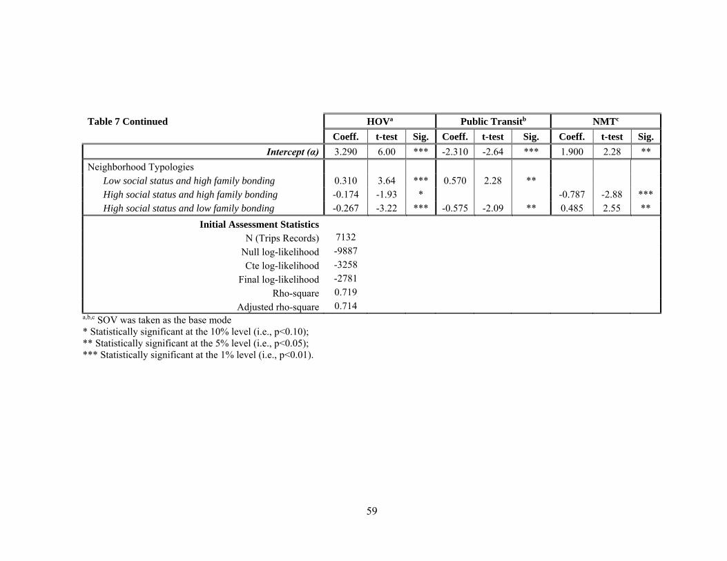
59
Table 7 Continued HOVa Public Transitb NMTc
Coeff. t-test Sig. Coeff. t-test Sig. Coeff. t-test Sig.
Intercept (α) 3.290 6.00 *** -2.310 -2.64 *** 1.900 2.28 **
Neighborhood Typologies Low social status and high family bonding 0.310 3.64 *** 0.570 2.28 ** High social status and high family bonding -0.174 -1.93 * -0.787 -2.88 *** High social status and low family bonding -0.267 -3.22 *** -0.575 -2.09 ** 0.485 2.55 **
Initial Assessment Statistics
N (Trips Records) 7132
Null log-likelihood -9887
Cte log-likelihood -3258
Final log-likelihood -2781
Rho-square 0.719
Adjusted rho-square 0.714 a,b,c SOV was taken as the base mode * Statistically significant at the 10% level (i.e., p<0.10); ** Statistically significant at the 5% level (i.e., p<0.05); *** Statistically significant at the 1% level (i.e., p<0.01).
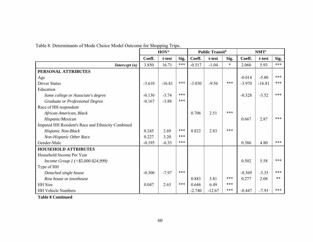
60
Table 8. Determinants of Mode Choice Model Outcome for Shopping Trips. HOVa Public Transitb NMTc
Coeff. t-test Sig. Coeff. t-test Sig. Coeff. t-test Sig.
Intercept (α) 3.850 16.71 *** -0.517 -1.04 * 2.060 5.93 ***
PERSONAL ATTRIBUTES Age -0.014 -5.80 *** Driver Status -3.610 -16.81 *** -3.030 -9.56 *** -3.970 -16.81 *** Education
Some college or Associate's degree -0.130 -3.74 *** -0.328 -3.52 *** Graduate or Professional Degree -0.167 -3.88 ***
Race of HH respondent African American, Black 0.706 2.51 *** Hispanic/Mexican 0.667 2.87 ***
Imputed HH Resident's Race and Ethnicity Combined Hispanic Non-Black 0.245 2.69 *** 0.822 2.83 *** Non-Hispanic Other Race 0.227 3.20 ***
Gender-Male -0.195 -6.35 *** 0.386 4.80 ***
HOUSEHOLD ATTRIBUTES Household Income Per Year
Income Group 1 (<$5,000-$24,999) 0.502 5.58 *** Type of HH
Detached single house -0.300 -7.97 *** -0.369 -3.35 *** Row house or townhouse 0.883 3.81 *** 0.277 2.08 **
HH Size 0.047 2.63 *** 0.646 6.49 *** HH Vehicle Numbers -2.740 -12.67 *** -0.447 -7.93 ***
Table 8 Continued

61
Table 8 Continued HOVa Public Transitb NMTc
Coeff. t-test Sig. Coeff. t-test Sig. Coeff. t-test Sig.
Intercept (α) 3.850 16.71 *** -0.517 -1.04 * 2.060 5.93 ***
HH Life Cycle One adult, no children -1.780 -20.11 *** 2+ adults, no children -0.461 -11.73 *** 2+ adults, youngest child 0-5 yrs 0.353 4.94 *** One adult, youngest child 6-15 yrs 0.795 2.37 ** 2+ adults, youngest child 6-15 yrs -1.910 -2.46 *** One adult, retired, no children -1.600 -24.21 ***
Total number of HH adult (18 years or older) members 0.336 6.52 *** Home Ownership (Home is owned) -0.825 -3.48 *** -0.270 -2.23 **
IMMIGRANT RELATED ATTRIBUTES Respondent is Immigrant/Foreign-born 0.133 2.819 *** 1.779 3.707 *** 0.187 1.64 * Arrival Time
Migrated 20 or more yrs ago 1.090 4.00 *** 0.334 3.25 *** Migrated >10 to 15 yrs ago 0.387 2.27 ** 1.216 3.372 *** Migrated >5 to 10 yrs ago 0.317 1.93 * 0.843 2.398 ** 0.684 2.224 ** Migrated 5 or less yrs ago 0.790 4.11 *** 1.071 2.11 ** 1.380 3.77 ***
LAND USE ATTRIBUTES Land Use Index Measurements
Entropy Index 1.420 2.86 *** 0.571 3.25 *** Measures of Attractiveness 0.187 4.785 *** 0.116 1.93 *
Table 8 Continued
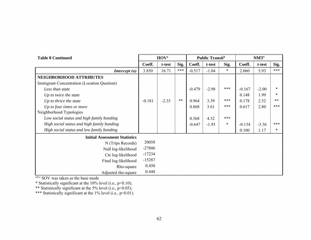
62
Table 8 Continued HOVa Public Transitb NMTc
Coeff. t-test Sig. Coeff. t-test Sig. Coeff. t-test Sig.
Intercept (α) 3.850 16.71 *** -0.517 -1.04 * 2.060 5.93 ***
NEIGHBORHOOD ATTRIBUTES Immigrant Concentration (Location Quotient)
Less than state -0.479 -2.98 *** -0.167 -2.00 * Up to twice the state 0.148 1.99 * Up to thrice the state -0.181 -2.35 ** 0.964 3.39 *** 0.178 2.52 ** Up to four times or more 0.868 3.61 *** 0.617 2.80 ***
Neighborhood Typologies Low social status and high family bonding 0.568 4.32 *** High social status and high family bonding -0.647 -1.93 * -0.134 -3.36 *** High social status and low family bonding 0.100 1.17 *
Initial Assessment Statistics N (Trips Records) 20058
Null log-likelihood -27806 Cte log-likelihood -17234
Final log-likelihood -15287 Rho-square 0.450
Adjusted rho-square 0.448 a,b,c SOV was taken as the base mode * Statistically significant at the 10% level (i.e., p<0.10); ** Statistically significant at the 5% level (i.e., p<0.05); *** Statistically significant at the 1% level (i.e., p<0.01).
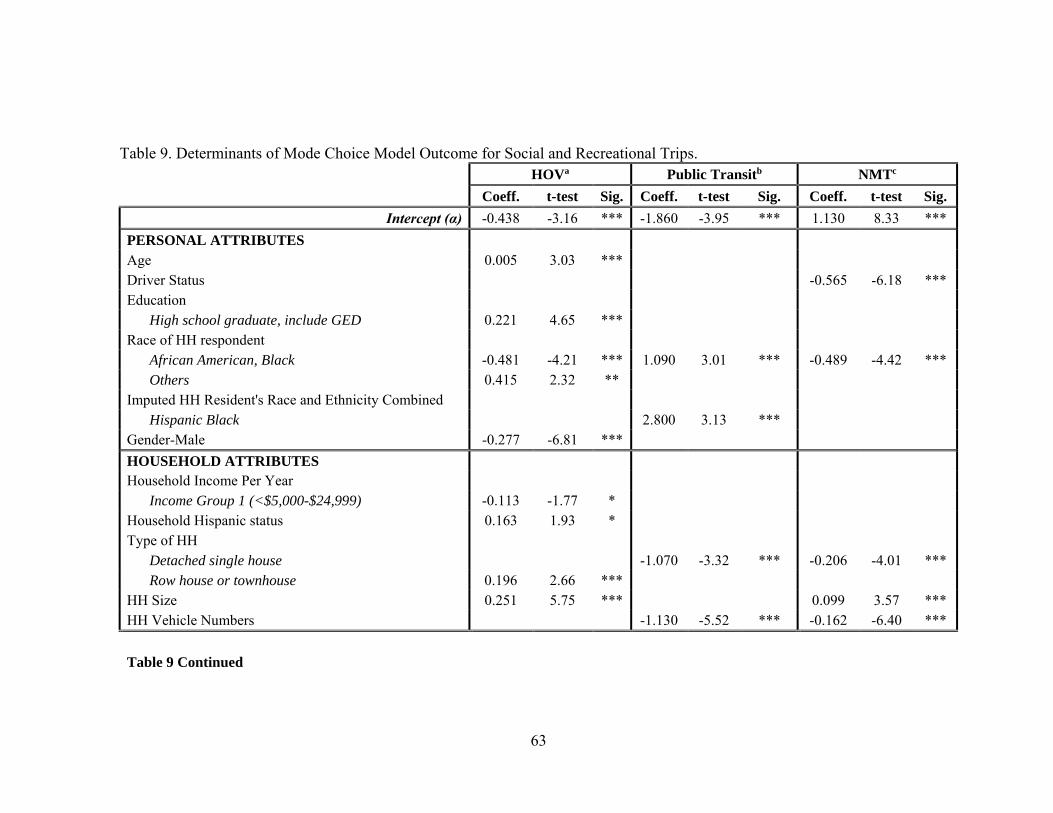
63
Table 9. Determinants of Mode Choice Model Outcome for Social and Recreational Trips. HOVa Public Transitb NMTc
Coeff. t-test Sig. Coeff. t-test Sig. Coeff. t-test Sig.
Intercept (α) -0.438 -3.16 *** -1.860 -3.95 *** 1.130 8.33 ***
PERSONAL ATTRIBUTES Age 0.005 3.03 *** Driver Status -0.565 -6.18 *** Education
High school graduate, include GED 0.221 4.65 *** Race of HH respondent
African American, Black -0.481 -4.21 *** 1.090 3.01 *** -0.489 -4.42 *** Others 0.415 2.32 **
Imputed HH Resident's Race and Ethnicity Combined Hispanic Black 2.800 3.13 ***
Gender-Male -0.277 -6.81 ***
HOUSEHOLD ATTRIBUTES Household Income Per Year
Income Group 1 (<$5,000-$24,999) -0.113 -1.77 * Household Hispanic status 0.163 1.93 * Type of HH
Detached single house -1.070 -3.32 *** -0.206 -4.01 *** Row house or townhouse 0.196 2.66 ***
HH Size 0.251 5.75 *** 0.099 3.57 *** HH Vehicle Numbers -1.130 -5.52 *** -0.162 -6.40 ***
Table 9 Continued
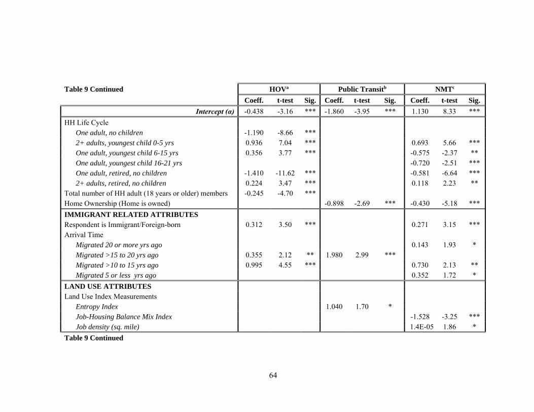
64
Table 9 Continued HOVa Public Transitb NMTc
Coeff. t-test Sig. Coeff. t-test Sig. Coeff. t-test Sig.
Intercept (α) -0.438 -3.16 *** -1.860 -3.95 *** 1.130 8.33 ***
HH Life Cycle One adult, no children -1.190 -8.66 *** 2+ adults, youngest child 0-5 yrs 0.936 7.04 *** 0.693 5.66 *** One adult, youngest child 6-15 yrs 0.356 3.77 *** -0.575 -2.37 ** One adult, youngest child 16-21 yrs -0.720 -2.51 *** One adult, retired, no children -1.410 -11.62 *** -0.581 -6.64 *** 2+ adults, retired, no children 0.224 3.47 *** 0.118 2.23 **
Total number of HH adult (18 years or older) members -0.245 -4.70 *** Home Ownership (Home is owned) -0.898 -2.69 *** -0.430 -5.18 ***
IMMIGRANT RELATED ATTRIBUTES Respondent is Immigrant/Foreign-born 0.312 3.50 *** 0.271 3.15 *** Arrival Time
Migrated 20 or more yrs ago 0.143 1.93 * Migrated >15 to 20 yrs ago 0.355 2.12 ** 1.980 2.99 *** Migrated >10 to 15 yrs ago 0.995 4.55 *** 0.730 2.13 ** Migrated 5 or less yrs ago 0.352 1.72 *
LAND USE ATTRIBUTES Land Use Index Measurements
Entropy Index 1.040 1.70 * Job-Housing Balance Mix Index -1.528 -3.25 *** Job density (sq. mile) 1.4E-05 1.86 *
Table 9 Continued

65
Table 9 Continued HOVa Public Transitb NMTc
Coeff. t-test Sig. Coeff. t-test Sig. Coeff. t-test Sig.
Intercept (α) -0.438 -3.16 *** -1.860 -3.95 *** 1.130 8.33 ***
NEIGHBORHOOD ATTRIBUTES Immigrant Concentration (Location Quotient)
Less than state -0.115 -2.23 ** Up to twice the state 0.093 2.00 *
Neighborhood Typologies Low social status and high family bonding 0.199 3.65 *** 0.095 1.97 * High social status and high family bonding 0.125 2.36 ** -0.982 -2.06 ** High social status and low family bonding -0.190 -2.98 *** Extremely low social status and low family bonding 1.267 2.45 ** -1.010 -4.06 ***
Initial Assessment Statistics N (Trips Records) 11753
Null log-likelihood -16293 Cte log-likelihood -13214
Final log-likelihood -12541 Rho-square 0.230
Adjusted rho-square 0.227 a,b,c SOV was taken as the base mode * Statistically significant at the 10% level (i.e., p<0.10); ** Statistically significant at the 5% level (i.e., p<0.05); *** Statistically significant at the 1% level (i.e., p<0.01).
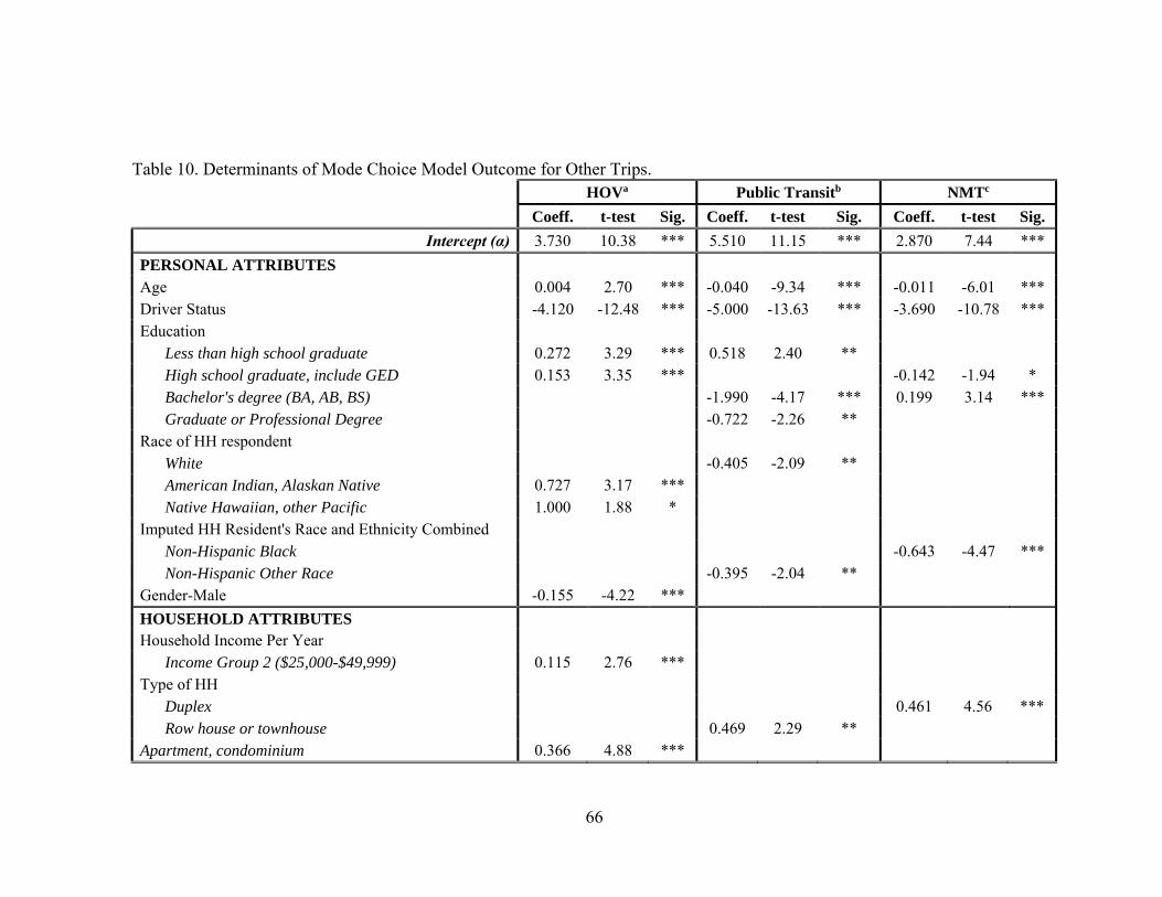
66
Table 10. Determinants of Mode Choice Model Outcome for Other Trips. HOVa Public Transitb NMTc
Coeff. t-test Sig. Coeff. t-test Sig. Coeff. t-test Sig.
Intercept (α) 3.730 10.38 *** 5.510 11.15 *** 2.870 7.44 ***
PERSONAL ATTRIBUTES Age 0.004 2.70 *** -0.040 -9.34 *** -0.011 -6.01 *** Driver Status -4.120 -12.48 *** -5.000 -13.63 *** -3.690 -10.78 *** Education
Less than high school graduate 0.272 3.29 *** 0.518 2.40 ** High school graduate, include GED 0.153 3.35 *** -0.142 -1.94 * Bachelor's degree (BA, AB, BS) -1.990 -4.17 *** 0.199 3.14 *** Graduate or Professional Degree -0.722 -2.26 **
Race of HH respondent White -0.405 -2.09 ** American Indian, Alaskan Native 0.727 3.17 *** Native Hawaiian, other Pacific 1.000 1.88 *
Imputed HH Resident's Race and Ethnicity Combined Non-Hispanic Black -0.643 -4.47 *** Non-Hispanic Other Race -0.395 -2.04 **
Gender-Male -0.155 -4.22 ***
HOUSEHOLD ATTRIBUTES Household Income Per Year
Income Group 2 ($25,000-$49,999) 0.115 2.76 *** Type of HH
Duplex 0.461 4.56 *** Row house or townhouse 0.469 2.29 **
Apartment, condominium 0.366 4.88 ***
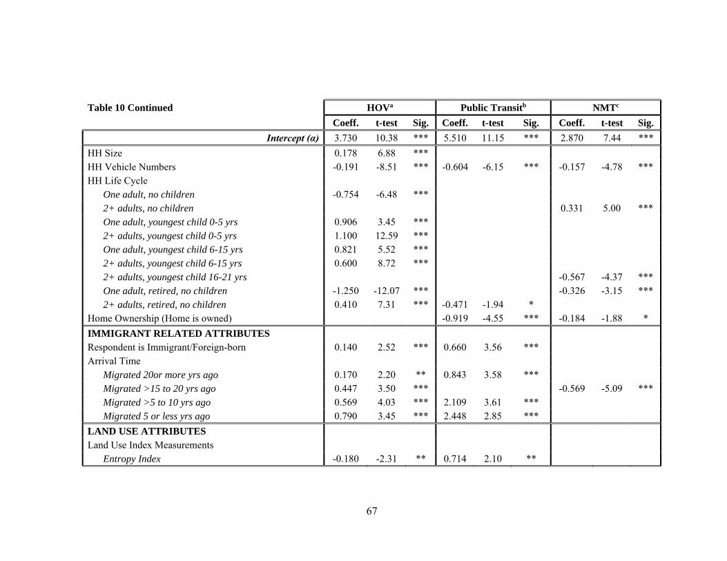
67
Table 10 Continued HOVa Public Transitb NMTc
Coeff. t-test Sig. Coeff. t-test Sig. Coeff. t-test Sig.
Intercept (α) 3.730 10.38 *** 5.510 11.15 *** 2.870 7.44 ***
HH Size 0.178 6.88 *** HH Vehicle Numbers -0.191 -8.51 *** -0.604 -6.15 *** -0.157 -4.78 *** HH Life Cycle
One adult, no children -0.754 -6.48 *** 2+ adults, no children 0.331 5.00 *** One adult, youngest child 0-5 yrs 0.906 3.45 *** 2+ adults, youngest child 0-5 yrs 1.100 12.59 *** One adult, youngest child 6-15 yrs 0.821 5.52 *** 2+ adults, youngest child 6-15 yrs 0.600 8.72 *** 2+ adults, youngest child 16-21 yrs -0.567 -4.37 *** One adult, retired, no children -1.250 -12.07 *** -0.326 -3.15 *** 2+ adults, retired, no children 0.410 7.31 *** -0.471 -1.94 *
Home Ownership (Home is owned) -0.919 -4.55 *** -0.184 -1.88 *
IMMIGRANT RELATED ATTRIBUTES Respondent is Immigrant/Foreign-born 0.140 2.52 *** 0.660 3.56 *** Arrival Time
Migrated 20or more yrs ago 0.170 2.20 ** 0.843 3.58 *** Migrated >15 to 20 yrs ago 0.447 3.50 *** -0.569 -5.09 *** Migrated >5 to 10 yrs ago 0.569 4.03 *** 2.109 3.61 *** Migrated 5 or less yrs ago 0.790 3.45 *** 2.448 2.85 ***
LAND USE ATTRIBUTES Land Use Index Measurements
Entropy Index -0.180 -2.31 ** 0.714 2.10 **
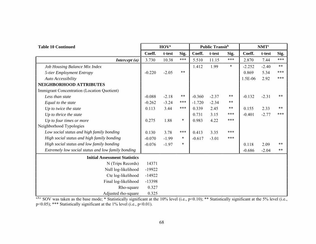
68
Table 10 Continued HOVa Public Transitb NMTc
Coeff. t-test Sig. Coeff. t-test Sig. Coeff. t-test Sig.
Intercept (α) 3.730 10.38 *** 5.510 11.15 *** 2.870 7.44 ***
Job Housing Balance Mix Index 1.412 1.99 * -2.252 -2.40 ** 5-tier Employment Entropy -0.220 -2.05 ** 0.869 5.34 *** Auto Accessibility 1.5E-06 2.92 ***
NEIGHBORHOOD ATTRIBUTES Immigrant Concentration (Location Quotient)
Less than state -0.088 -2.18 ** -0.360 -2.37 ** -0.132 -2.31 ** Equal to the state -0.262 -3.24 *** -1.720 -2.34 ** Up to twice the state 0.113 3.44 *** 0.339 2.45 ** 0.155 2.33 ** Up to thrice the state 0.731 3.15 *** -0.401 -2.77 *** Up to four times or more 0.275 1.88 * 0.983 4.22 ***
Neighborhood Typologies Low social status and high family bonding 0.130 3.78 *** 0.413 3.35 *** High social status and high family bonding -0.070 -1.99 * -0.617 -3.01 *** High social status and low family bonding -0.076 -1.97 * 0.118 2.09 ** Extremely low social status and low family bonding -0.686 -2.04 **
Initial Assessment Statistics N (Trips Records) 14371
Null log-likelihood -19922 Cte log-likelihood -14922
Final log-likelihood -13398 Rho-square 0.327
Adjusted rho-square 0.325 a,b,c SOV was taken as the base mode; * Statistically significant at the 10% level (i.e., p<0.10); ** Statistically significant at the 5% level (i.e., p<0.05); *** Statistically significant at the 1% level (i.e., p<0.01).
69
The coefficients of determinants are statistically significant, at least at the 10%
level. The significance levels are indicated in all of the tables as * p<0.10; ** p<0.05; and
*** p<0.01. In most of the cases, the estimated results indicate a 99% confidence level.
The lower values of standard error refer to the higher precision of the estimated co-
efficient. The absolute values of the t-test are found to be sufficiently large, which leads
to the rejection of the null hypothesis that the parameter is equal to the hypothesized
value. The rejection of the null hypothesis implies that the corresponding variable has a
significant impact on the modal utilities and suggests that the variable should be retained
in the model. Low absolute values of the t-test imply that the variables do not contribute
significantly to the explanatory power of the model and can be considered for exclusion.
The following section addresses the models’ outputs based on immigrants’ trips for work,
shopping, social, recreational, and other purposes.
5.1. Individual Attributes
Coefficients of the mode choice determinants indicate that the increase in trip makers’
age has a positive impact on SOV usage over carpooling or non-motorized modes for
work and shopping trips. It may be because individuals gain more economic stability
while aging. There is also an increased rate of driving license holders among the elderly.
People that have a driver’s license are more willing to drive alone irrespective of any trip
purposes. Both economic stability and possession of a driver’s license contribute to the
opportunity of possessing a private vehicle. Moreover, an elderly trip maker may find it
more convenient to commute to their place of employment by driving their own vehicle
rather than seeking help or waiting for carpool or shared rides. Tables 7 through 10 imply
70
the favored SOV usage over the other three modes of transportation when individuals
possess a driver’s license. The possession of a legal license influences the majority of
drivers to drive alone for work trips; their secondary preference is public transit. They
find it more convenient to drive by them over worrying about whether or not transit or
NMT is reliable or over carpooling to save time. These facts make it clearer that legality
issues are truly concerned with people’s choice of modes [15]. However, for shopping,
recreational, and other trips, they prefer non-motorized modes next to solo driving.
Gender issue also influences people’s chosen mode of transportation. For any trip
purpose, male individuals choose SOV over any other mode of transportation. Previous
studies indicate that more males are driving license holders, compared to the females
[15].
People of the white race are more likely to drive alone to work and shopping trips.
However, the African American race is more inclined to use public transit for work,
shopping, and recreational trips. Earlier studies have reported race-based mode choice
preference. The white race is economically more affluent than other groups and this
influences their mode choice preference [17, 71]. Racial or ethnic difference is a
significant indicator for all trip purposes in this current study. Hispanic households, either
African-American or not, prefer public transit, whereas non-Hispanic/other races choose
carpooling or SOV.
People that have earned a high school degree are less are likely to use carpool or
shared rides than SOV. The decrease of coefficients from 0.753 (less than a high school
graduate) to 0.270 (high school graduate) for work trips (Table 7) indicates the steady
shift in preference from HOV to SOV. The same holds true for other trip purposes (Table
71
10); the public transit usage decreases with superior educational qualifications that stem
from estimated coefficients of 0.518, -1.990, and -0.722 for less than high school
graduates, high school graduates, and graduate or professional degree holders,
respectively. This may be because with higher educational attainment, people have better
paying jobs, which decreases their likelihood to carpool or share rides.
5.2. Household Attributes
The income group has a versatile scenario in the case of work trips. For example, for
work trips, people of household yearly incomes of $50,000 to $74,999 prefer
carpooling/ride sharing. They may live far from downtown areas and live in single homes
and may have to travel higher vehicle miles to reach their place of employment. In these
cases, this income group finds HOV usage to be cost-effective, convenient, and reliable.
In most cases, the lowest income group (<$5,000 to $24,999/ year) has a higher
propensity toward the alternative modes over SOV. The use of public transit shifts
towards solo driving with the increase of income.
People living in detached single homes are more likely to drive alone than
carpooling and NMT for work, shopping, and recreational trips. Apartment or
condominium house residents are more likely to take public transit than SOV. For
example, mode choice determinants of household members living in row or town housing
have shown a strong inclination toward alternative modes over driving alone. These facts
also support the reality that the single detached households situated in more aesthetic
areas are generally owned by wealthier people, who generally have a comparatively
higher rate of vehicle ownership than the residents of apartments, condominiums, or
72
townhouse inhabitants. These factors make them more likely to drive alone. An increase
in the number of household vehicles influences the use of SOVs for any trip purposes
[17].
The number of adult family members increases the likelihood of driving alone
over carpooling/ride sharing (Table 9). More adult members in the household may be an
indication of an increase in earnings, as well as being more financially stable. Increase in
the household size favors carpooling or ride sharing for all other trips except work trips.
Larger households are composed of more family members that may include children,
senior citizens, more than one adult, etc. However, they may not include more earning
members or family members with higher salaries or higher car ownership. They may
prefer to travel altogether simply because of their family bonding. Homeowners are
economically better off and prefer to drive alone irrespective of any trip purposes. Their
secondary preference is NMT before public transit.
Individuals from the households with children aging 15 years or younger are
more likely to carpool, whereas existence of children aging 16-21 years old make the
household members to prefer SOV. In general, adults that have no children prefer SOV.
The household life cycle shows the relationship between lifestyle and chosen modes. For
work trips, trip makers of households with one adult and no children are more likely to
drive alone; the secondary preference is non-motorized modes. The underlying reason
may be that they do not have to drop off the children to school while on their way to
work and/or they live near schools. The households having more than two adults with
children increase the propensity of its members to use carpooling/ride sharing. For
shopping trips, a trend is seen where households with children increase the likelihood of
73
HOV usage, whereas trip makers from the households of one adult (irrespective of retired
or employed) having no children, which further increases the likelihood to drive alone.
5.3. Immigrant-related Attributes
Previous researches support that foreign-born people or immigrants unlike the US-born
individuals are more likely to use alternative modes of transportation (carpooling/ride
sharing, public transit, and non-motorized modes) other than solo driving for all trip
purposes [5-8] [12, 14, 16-19]. For work and shopping trips, they are less likely to
carpool than use public transit and NMT. It may be because obtaining a ride from
someone else is not always possible, or they live near their place of employment and
shopping areas.
Immigrants’ arrival period in the US has a significant influence on mode choice.
For example, immigrants that migrated >15-19 years ago are more likely to drive alone.
The behavioral assimilation analysis in Chapter 3 showed that immigrants that migrated
>10 to 15 years ago are more economically sound than those arriving 20 or more years
ago. The second group is comprised of senior citizens, mostly retirees. Their age,
physical condition, household status, and economic stability make them likely to access
HOV over driving alone. The observed trend is that except for immigrants that migrated
>15 to 19 years ago, all are positively inclined toward carpooling/ride sharing, and the
likelihood is higher among recent immigrants, i.e., those who migrated within the last 5
years (0.664), between >5-10 years (0.664), and 20 or more years ago (0.379). A similar
trend is seen in terms of public transit usage. For shopping trips, the immigrants arriving
within the last 5 years have the highest likelihood toward HOV, PT, and NMT, compared
74
to others arriving earlier. Immigrants prefer alternative modes of transportation to go
shopping or take recreational trips rather than drive alone, irrespective of how many years
they have lived in the U.S. For recreational trips, their preference is slightly more for
public transportation over carpooling or NMT, and those arriving more than 20 years ago
have the lowest likelihood toward the other three modes, compared to driving alone. The
similar trend is seen in the case of other, i.e., school, maintenance, personal business,
religious trips (Table 10). With ample time spent time in the U.S., their preference toward
the use of HOV, PT, and NMT decreases, and again, the immigrants arriving >15 to 19
years ago prefer to drive alone over NMT usage. However, the most economically stable
individuals for shopping and social-recreational trips are more likely to use alternate
modes over SOV since recreational trips are normally made with friends or family.
5.4. Land Use Attributes
In terms of work trips, the employment entropy index increases the likelihood of
carpooling or ride sharing. It may indicates that a balanced distribution of jobs help
people save time and avoid time overlapping to obtain rides. The measures of
attractiveness indicate the distribution of places of interest works and have the positive
influence on public transit usage. This may indicate that areas that have higher points of
interest also hold a higher provision of transit services. For shopping trips, both the
entropy index and measures of attractiveness increase the propensity to use public transit
and non-motorized modes; though the entropy index’s higher value indicates a higher
degree of influence. Therefore, the more the mixed land use is equipped with points of
interest and transit services, the more people become open to using alternative modes of
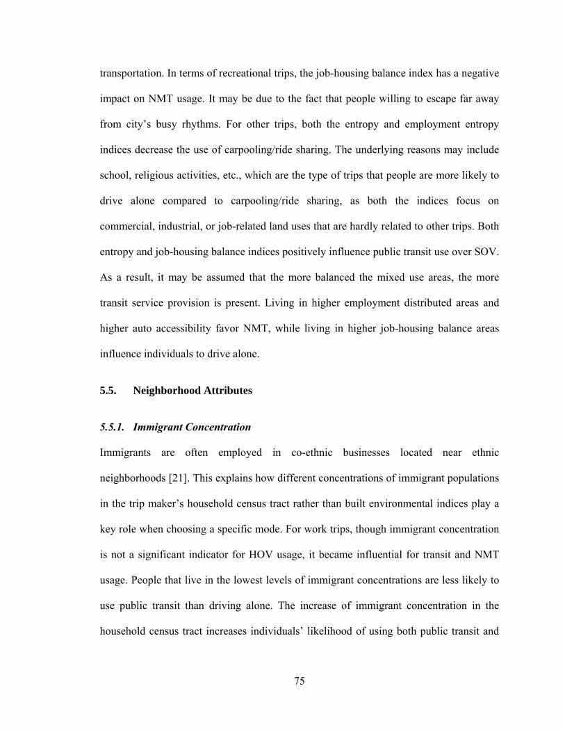
75
transportation. In terms of recreational trips, the job-housing balance index has a negative
impact on NMT usage. It may be due to the fact that people willing to escape far away
from city’s busy rhythms. For other trips, both the entropy and employment entropy
indices decrease the use of carpooling/ride sharing. The underlying reasons may include
school, religious activities, etc., which are the type of trips that people are more likely to
drive alone compared to carpooling/ride sharing, as both the indices focus on
commercial, industrial, or job-related land uses that are hardly related to other trips. Both
entropy and job-housing balance indices positively influence public transit use over SOV.
As a result, it may be assumed that the more balanced the mixed use areas, the more
transit service provision is present. Living in higher employment distributed areas and
higher auto accessibility favor NMT, while living in higher job-housing balance areas
influence individuals to drive alone.
5.5. Neighborhood Attributes
5.5.1. Immigrant Concentration
Immigrants are often employed in co-ethnic businesses located near ethnic
neighborhoods [21]. This explains how different concentrations of immigrant populations
in the trip maker’s household census tract rather than built environmental indices play a
key role when choosing a specific mode. For work trips, though immigrant concentration
is not a significant indicator for HOV usage, it became influential for transit and NMT
usage. People that live in the lowest levels of immigrant concentrations are less likely to
use public transit than driving alone. The increase of immigrant concentration in the
household census tract increases individuals’ likelihood of using both public transit and
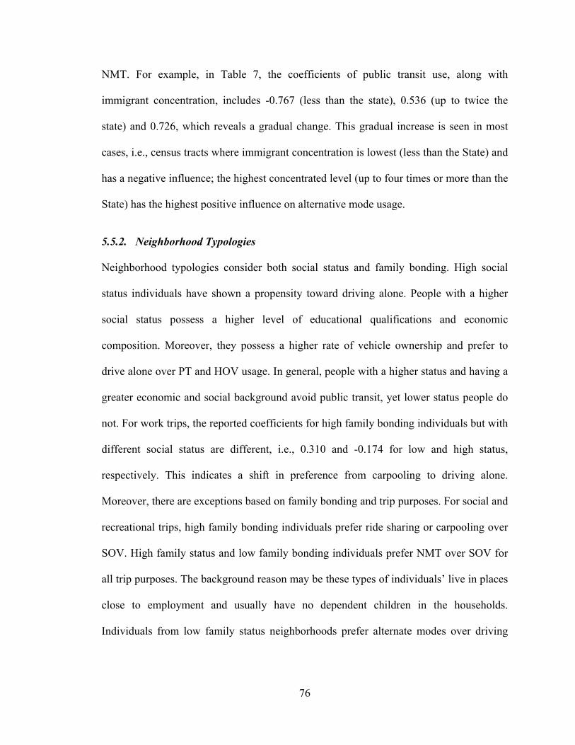
76
NMT. For example, in Table 7, the coefficients of public transit use, along with
immigrant concentration, includes -0.767 (less than the state), 0.536 (up to twice the
state) and 0.726, which reveals a gradual change. This gradual increase is seen in most
cases, i.e., census tracts where immigrant concentration is lowest (less than the State) and
has a negative influence; the highest concentrated level (up to four times or more than the
State) has the highest positive influence on alternative mode usage.
5.5.2. Neighborhood Typologies
Neighborhood typologies consider both social status and family bonding. High social
status individuals have shown a propensity toward driving alone. People with a higher
social status possess a higher level of educational qualifications and economic
composition. Moreover, they possess a higher rate of vehicle ownership and prefer to
drive alone over PT and HOV usage. In general, people with a higher status and having a
greater economic and social background avoid public transit, yet lower status people do
not. For work trips, the reported coefficients for high family bonding individuals but with
different social status are different, i.e., 0.310 and -0.174 for low and high status,
respectively. This indicates a shift in preference from carpooling to driving alone.
Moreover, there are exceptions based on family bonding and trip purposes. For social and
recreational trips, high family bonding individuals prefer ride sharing or carpooling over
SOV. High family status and low family bonding individuals prefer NMT over SOV for
all trip purposes. The background reason may be these types of individuals’ live in places
close to employment and usually have no dependent children in the households.
Individuals from low family status neighborhoods prefer alternate modes over driving

77
alone, irrespective of trip purposes. Among alternate modes, they are inclined toward
using public transit and carpooling for work and other trips. The relevant coefficients are
0.570 over 0.310; and 0.413 over 0.130 for work and other trips, respectively. People
from neighborhoods of low social status and high family bonding prefer HOV. Either
they like to travel around with their family members or have a lower rate of private
vehicle ownership. The change in extremely low status and bonding move their
preference towards driving alone for other trips. People who are alone with a low family
bonding and who live in extremely low status neighborhoods may prefer to drive alone
for other trips that involve concern for safety or security. For recreational trips, they
prefer public transit and driving alone and may hardly get anyone to accompany them. In
short, people living in neighborhoods with a higher social status always prefer to drive
alone over HOV or public transit usage, though the preference leans toward the latter two
alternative modes with the lowering of status and the increase of family bonding.
5.6. Summary
Immigrant-related attributes and neighborhood attributes are significant predictors of
immigrants’ travel mode choice; even the traditionally used indicators are often found to
be insignificant. Carpooling/ride sharing is an indication of the social relationship among
kin and friends. There are notable impacts of additional built environment patterns and
location quotient of immigrant population on their travel behavior. The foreign-born
status and arrival period also significantly change trip pattern. Therefore, aggregation of
all of the possible attributes and relevant variables will show the interrelationships among
immigrants and will better reflect their travel behavior.
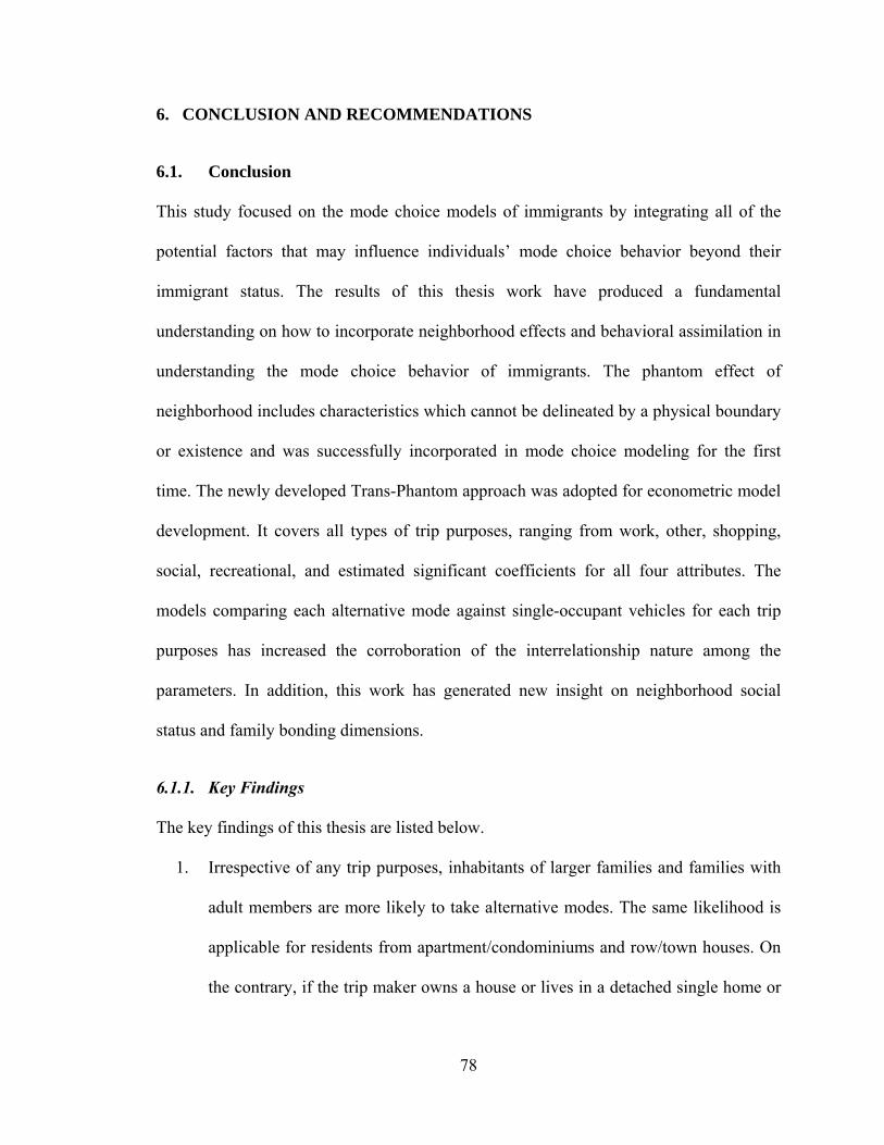
78
6. CONCLUSION AND RECOMMENDATIONS
6.1. Conclusion
This study focused on the mode choice models of immigrants by integrating all of the
potential factors that may influence individuals’ mode choice behavior beyond their
immigrant status. The results of this thesis work have produced a fundamental
understanding on how to incorporate neighborhood effects and behavioral assimilation in
understanding the mode choice behavior of immigrants. The phantom effect of
neighborhood includes characteristics which cannot be delineated by a physical boundary
or existence and was successfully incorporated in mode choice modeling for the first
time. The newly developed Trans-Phantom approach was adopted for econometric model
development. It covers all types of trip purposes, ranging from work, other, shopping,
social, recreational, and estimated significant coefficients for all four attributes. The
models comparing each alternative mode against single-occupant vehicles for each trip
purposes has increased the corroboration of the interrelationship nature among the
parameters. In addition, this work has generated new insight on neighborhood social
status and family bonding dimensions.
6.1.1. Key Findings
The key findings of this thesis are listed below.
1. Irrespective of any trip purposes, inhabitants of larger families and families with
adult members are more likely to take alternative modes. The same likelihood is
applicable for residents from apartment/condominiums and row/town houses. On
the contrary, if the trip maker owns a house or lives in a detached single home or

79
has a higher yearly income or has a number of household vehicles, then the
individual is more likely to choose driving alone over the alternative modes.
Hispanic households prefer carpooling or ridesharing than SOV. A household life
cycle was shown to be a significant indicator in all of the models, though past
research hardly integrated this household attribute. A household comprised of
dependent children make their family members choose carpool/ridesharing over
driving alone, and one or more adult members living without any children prefer
to drive alone.
2. Foreign-born individuals are more likely to use alternative modes of
transportation than US-born individuals, and their migrating period in the US has
significant influence on their mode choice behavior. Foreign-born immigrants,
excluding those that arrived >10 to 15 years ago, always prefer alternative modes
for all trip purposes. The most economically stable group prefers driving alone for
work trips over alternate modes. However, for shopping and social-recreational
trips, they are more likely to use alternate modes over SOV.
3. Immigrant quotient was redefined in this study. The new method of grouping
provides better insight on travel behavior. The propensity of transit and NMT
usage increases with the increase of immigrant percentage in the household
census tract.
4. Individuals’ mode choice for trips is influenced by the neighborhood typologies,
i.e., social status and family bonding. They prefer driving alone or using alternate
modes, depending on high or low status, respectively. High family bonding for

80
high social status favors carpooling for social and recreational trips. Extremely
low family status and low family bonding individuals prefer driving alone.
6.1.2. Accomplishments
The accomplishments of this thesis include: Incorporation of new variables for
individual, household, immigrant, and neighborhood attributes; inclusion of
neighborhood social status and family bonding context; development of mode choice
models considering both neighborhood effects and behavioral assimilation; introduction
of the Trans-Phantom approach in mode choice modeling; trip purpose-based mode
choice; attribute-based mode choice irrespective of any trip; and estimated coefficients
for significant attributes-variables-categories. Furthermore, the results also present a
more challenging way to tackle the diversified complexity of travel behavior, especially
for non-US-born individuals in the US.
Overall, the results from this thesis highlight the importance of new variables in
understanding immigrants’ mode choice behavior. It is imperative that each choice of
travel modes shares its compatibility issues with different land use patterns, auto
ownership, and people of versatile backgrounds, characteristics, social status, and family
ties for the various trip purposes. The resultant models of this study precede the new
dimensions of people’s mode choice behavior integrating the neighborhood and built
environment extents. The estimates of transit ridership and the alternative mode usage
can be used in future transportation policy planning relevant to immigrant population at
the regional or state level.
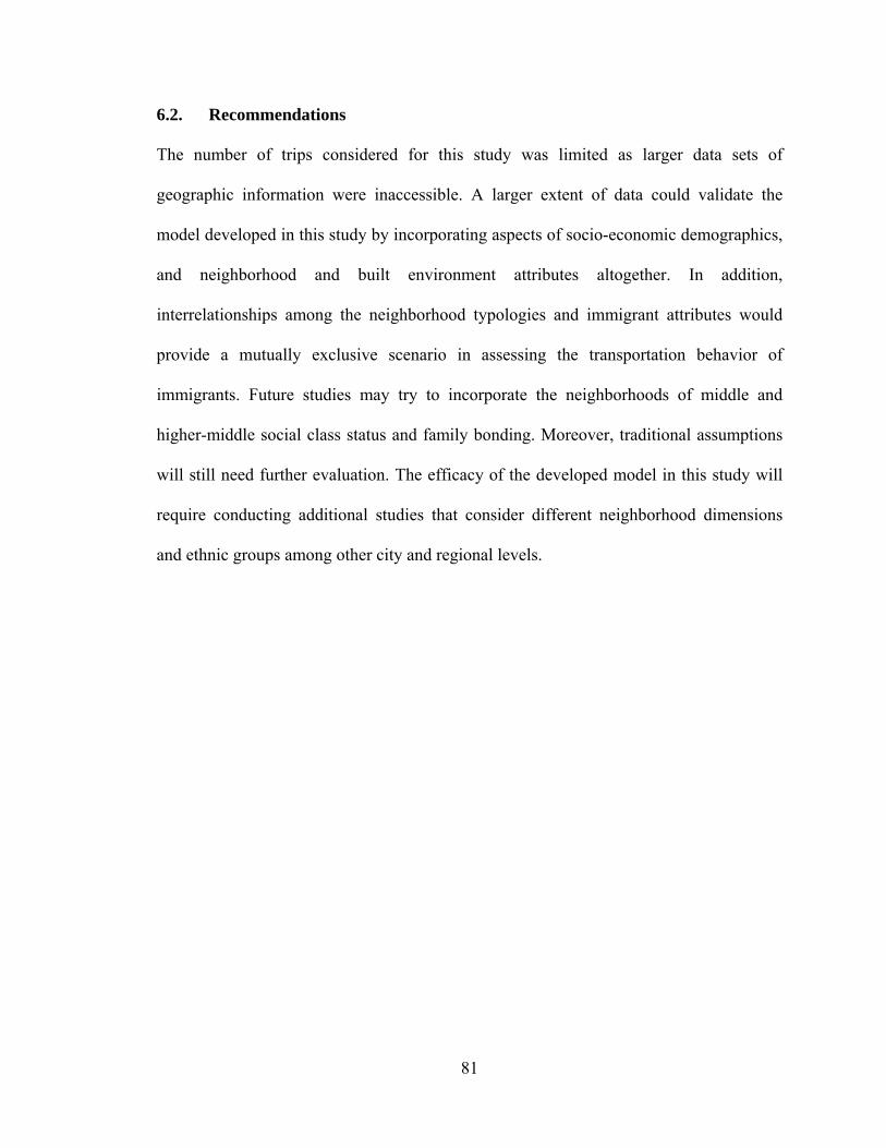
81
6.2. Recommendations
The number of trips considered for this study was limited as larger data sets of
geographic information were inaccessible. A larger extent of data could validate the
model developed in this study by incorporating aspects of socio-economic demographics,
and neighborhood and built environment attributes altogether. In addition,
interrelationships among the neighborhood typologies and immigrant attributes would
provide a mutually exclusive scenario in assessing the transportation behavior of
immigrants. Future studies may try to incorporate the neighborhoods of middle and
higher-middle social class status and family bonding. Moreover, traditional assumptions
will still need further evaluation. The efficacy of the developed model in this study will
require conducting additional studies that consider different neighborhood dimensions
and ethnic groups among other city and regional levels.
82
REFERENCES
1. Massey, D.S., et al., Theories of international migration: a review and appraisal. Population and Development Review, 1993: p. 431-466.
2. Passel, J.S. and D.V. Cohn, A Portrait of unauthorized immigrants in the United States. 2009, Pew Hispanic Center: Washington, DC.
3. Martin, P. and E. Midgley, Population bulletin update: immigration in America 2010. 2010, Population Reference Bureau.
4. Batalova, J., Immigrants in the U.S. labor force, in U.S. Immigration Trends. 2014, Migration Policy Institute: Washington, DC.
5. Blumenberg, E., Moving in and moving around: immigrants, travel behavior, and implications for transport policy. Transportation Letters, 2009. 1(2): p. 169-180.
6. Burbidge, S.K., Foreign living experience as a predictor of domestic travel behavior. Journal of Transport Geography, 2012. 22: p. 199-205.
7. Casas, J., C. Arce, and C. Frye, Latino immigration and its impact on future travel behavior, in National Household Travel Survey Conference: Understanding Our Nation’s Travel, Washington, DC. 2004.
8. Handy, S., et al., Travel behavior of Mexican and other immigrant groups in California. Berkeley Planning Journal, 2008. 21(1): p. 1-24.
9. Batalova, J., State Immigrantion Data Profile, in Data Hub-U.S. Data, J. Batalova, Editor. 2014, Migration Policy Institute: Washington, DC.
10. Eisenhauer, E., et al., Immigrants in Florida: characteristics and contributions. 2007, Research Institute for Social and Economic Policy (RISEP), FIU: Miami, FL, USA.
11. Crane, R. and R. Crepeau, Does neighborhood design influence travel?: A behavioral analysis of travel diary and GIS data. Transportation Research Part D: Transport and Environment, 1998. 3(4): p. 225-238.
12. Blumenberg, E. and M. Smart, Getting by with a little help from my friends… and family: immigrants and carpooling. Transportation, 2010. 37(3): p. 429-446.
83
13. Bagley, M.N. and P.L. Mokhtarian, The impact of residential neighborhood type on travel behavior: a structural equations modeling approach. The Annals of Regional Science, 2002. 36(2): p. 279-297.
14. Smart, M.J., A nationwide look at the immigrant neighborhood effect on travel mode choice. Transportation, 2014. 41: p. 1-21.
15. Blumenberg, E., Immigrants and transport barriers to employment: The case of Southeast Asian welfare recipients in California. Transport Policy, 2008. 15(1): p. 33-42.
16. Smart, M.J., US immigrants and bicycling: Two-wheeled in Autopia. Transport Policy, 2010. 17(3): p. 153-159.
17. Tal, G. and S. Handy, Travel behavior of immigrants: An analysis of the 2001 National Household Transportation Survey. Transport Policy, 2010. 17(2): p. 85-93.
18. Liu, C.Y. and G. Painter, Travel Behavior among Latino immigrants: the role of ethnic concentration and ethnic employment. Journal of Planning Education and Research, 2012. 32(1): p. 62-80.
19. Blumenberg, E. and M. Smart, Brother can you spare a ride? Carpooling in immigrant neighbourhoods. Urban Studies, 2014. 51(9): p. 1871-1890.
20. Alba, R.D., J.R. Logan, and B.J. Stults, The changing neighborhood contexts of the immigrant metropolis. Social Forces, 2000. 79(2): p. 587-621.
21. Blumenberg, E. and M. Smart, Travel in the’hood: ethnic neighborhoods and mode choice. University of California Transportation Center, 2009.
22. Lovejoy, K. and S. Handy, Social networks as a source of private-vehicle transportation: The practice of getting rides and borrowing vehicles among Mexican immigrants in California. Transportation Research Part A: Policy and Practice, 2011. 45(4): p. 248-257.
23. Logan, J.R., W. Zhang, and R.D. Alba, Immigrant enclaves and ethnic communities in New York and Los Angeles. American Sociological Review, 2002: p. 299-322.
24. Bhat, C.R. and J.Y. Guo, A comprehensive analysis of built environment characteristics on household residential choice and auto ownership levels. Transportation Research Part B: Methodological, 2007. 41(5): p. 506-526.
84
25. Yang, L., G. Zheng, and X. Zhu, Cross-nested logit model for the joint choice of residential location, travel mode, and departure time. Habitat International, 2013. 38: p. 157-166.
26. Frank, L.D. and G. Pivo, Impacts of mixed use and density on utilization of three modes of travel: single-occupant vehicle, transit, and walking. Transportation Research Record, 1994. 1466: p. 37-43.
27. Handy, S., X. Cao, and P. Mokhtarian, Correlation or causality between the built environment and travel behavior? Evidence from Northern California. Transportation Research Part D: Transport and Environment, 2005. 10(6): p. 427-444.
28. Kockelman, K.M., Travel behavior as function of accessibility, land use mixing, and land use balance: evidence from San Francisco Bay Area. Transportation Research Record, 1997. 1607(1): p. 116-125.
29. Krizek, K.J., Operationalizing neighborhood accessibility for land use-travel behavior research and regional modeling. Journal of Planning Education and Research, 2003. 22(3): p. 270-287.
30. Messenger, T. and R. Ewing, Transit-oriented development in the sun belt. Transportation Research Record, 1996. 1552(1): p. 145-153.
31. Cullen, I. and V. Godson, Urban networks: the structure of activity patterns. Progress in Planning, 1975. 4: p. 1-96.
32. Schoenberg, S.P., Criteria for the evaluation of neighborhood viability in working class and low income areas in core cities. Social Problems, 1979: p. 69-78.
33. Fischer, C.S., The study of urban community and personality. Annual Review of Sociology, 1975: p. 67-89.
34. Park, R.E., The city: suggestions for the investigation of human behavior in the city environment. American Journal of Sociology, 1915. 20(5): p. 577-612.
35. Olson, P., Urban neighborhood research Its development and current focus. Urban Affairs Review, 1982. 17(4): p. 491-518.
36. Galster, G., On the nature of neighbourhood. Urban Studies, 2001. 38(12): p. 2111-2124.
85
37. Warren, D.I., Helping networks: How people cope with problems in the urban community. 1981, Notre Dame, IN: University of Notre Dame Press
38. Wellman, B., The community question: The intimate networks of East Yorkers. American Journal of Sociology, 1979: p. 1201-1231.
39. Chow, J., Differentiating urban neighborhoods: A multivariate structural model analysis. Social Work Research, 1998. 22(3): p. 131-142.
40. Li, Y.-S. and Y.-C. Chuang, Neighborhood effects on an individual’s health using neighborhood measurements developed by factor analysis and cluster analysis. Journal of Urban Health, 2009. 86(1): p. 5-18.
41. Ellen, I.G. and M.A. Turner, Does neighborhood matter? Assessing recent evidence. Housing Policy Debate, 1997. 8(4): p. 833-866.
42. Burton, L.M. and R.L. Jarrett, In the mix, yet on the margins: The place of families in urban neighborhood and child development research. Journal of Marriage and Family, 2000. 62(4): p. 1114-1135.
43. Clapp, J.M. and Y. Wang, Defining neighborhood boundaries: Are census tracts obsolete? Journal of Urban Economics, 2006. 59(2): p. 259-284.
44. Harding, C.P., Zachary Rupert ; Axhausen, Kay W, Neighborhood and regional effects on trip dispersal: case study using data from nine largest metropolitan regions in Switzerland, in TRB 2014 Annual Meeting. 2014: Washington DC.
45. Crane, J., The epidemic theory of ghettos and neighborhood effects on dropping out and teenage childbearing. American Journal of Sociology, 1991: p. 1226-1259.
46. Brooks-Gunn, J., et al., Do neighborhoods influence child and adolescent development? American Journal of Sociology, 1993: p. 353-395.
47. Coulton, C.J., et al., Mapping residents' perceptions of neighborhood boundaries: a methodological note. American Journal of Community Psychology, 2001. 29(2): p. 371-383.
48. Smart, M.J., Immigrant ethnic neighborhoods, inward focus, and travel mode choice, in Urban Planning. 2011, University of California Los Angeles.
86
49. Manaugh, K. and T. Kreider, What is mixed use? Presenting an interaction method for measuring land use mix. Journal of Transport and Land Use, 2013. 6(1): p. 63-72.
50. Marwasta, D., Yogyakarta urban growth versus smart growth: towards Yogyakarta slow city proposal, in To Solve Social Problem Through Art and Cultural Activities: Theory and Practice. 2010: Yogyakarta.
51. Litman, T. and R. Steele, How land use factors affect travel behavior, in Land use impacts on transport. 2005, Victoria Transport Policy Institute: Canada.
52. 2009 National Household Travel Survy FDOT File. 2009, U.S. Department of Transportation, Federal Highway Administration.
53. 2009 National Household Travel Survy User Guide. 2009, U.S. Department of Transportation, Federal Highway Administration. http://nhts.ornl.gov/2009/pub/UsersGuideV1.pdf (accessed June 2014).
54. U.S. Census Bureau. 2010 American Community Survey. http://factfinder2.census.gov/ (accessed June 2014).
55. Smart Location Data Base. U.S. EPA. http://www.epa.gov/smartgrowth/smartlocationdatabase.htm (accessed on June 2014).
56. Miller, V.P. and J.M. Quigley, Segregation by racial and demographic group: evidence from the San Francisco Bay Area. Urban Studies, 1990. 27(1): p. 3-21.
57. Armstrong, M., B. Sears, and F. Wen, The new economy and jobs/housing balance in Southern California. Southern California Association of Governments, 2001.
58. Cervero, R. and M. Duncan, Which reduces vehicle travel more: jobs-housing balance or retail-housing mixing? Journal of the American Planning Association, 2006. 72(4): p. 475-490.
59. Johnston, R.J., ed. Residential area characteristics: research methods for identifying urban sub-areas—social area analysis and factorial ecology. Social Areas in Cities, ed. D.T. Herbert and R.J. Johnston. Vol. 1. 1976, John Wiley and Sons: London. 193-235.
87
60. Sampson, R.J., J.D. Morenoff, and T. Gannon-Rowley, Assessing "Neighborhood Effects": social processes and new directions in research. Annual Review of Sociology, 2002: p. 443-478.
61. Mooi, E. and M. Sarstedt, Factor analysis, in A concise guide to market research: The process, data, and methods using IBM SPSS statistics. 2011, Springer Berlin Heidelberg. p. 201-236.
62. Pett, M.A., N.R. Lackey, and J.J. Sullivan, Making sense of factor analysis: The use of factor analysis for instrument development in health care research. 2003: SAGE Publications, Inc.
63. Rapkin, B.D. and D.A. Luke, Cluster analysis in community research: Epistemology and practice. American Journal of Community Psychology, 1993. 21(2): p. 247-277.
64. Mooi, E. and M. Sarstedt, Cluster analysis, in A concise guide to market research: The process, data, and methods using IBM SPSS statistics. 2011, Springer Berlin Heidelberg. p. 237-284.
65. Milligan, G.W. and M.C. Cooper, An examination of procedures for determining the number of clusters in a data set. Psychometrika, 1985. 50(2): p. 159-179.
66. Milligan, G.W. and M.C. Cooper, Methodology review: Clustering methods. Applied Psychological Measurement, 1987. 11(4): p. 329-354.
67. McIntyre, R.M. and R.K. Blashfield, A nearest-centroid technique for evaluating the minimum-variance clustering procedure. Multivariate Behavioral Research, 1980. 15(2): p. 225-238.
68. Punj, G. and D.W. Stewart, Cluster analysis in marketing research: review and suggestions for application. Journal of Marketing Research, 1983: p. 134-148.
69. Cohen, J., Weighted kappa:nNominal scale agreement provision for scaled disagreement or partial credit. Psychological Bulletin, 1968. 70(4): p. 213.
70. Kaiser, H.F., An index of factorial simplicity. Psychometrika, 1974. 39(1): p. 31-36.
71. Tal, G. and S.L. Handy, The travel behavior of immigrants and race/ethnicity groups: an analysis of the 2001 national household transportation survey. Institute of Transportation Studies, UC Davis, 2005.

88
72. Koppelman, F.S. and C. Bhat, A self instructing course in mode choice modeling: multinomial and nested logit models. US Department of Transportation, Federal Transit Administration, 2006. 31.
73. Enam, A. and C.F. Choudhury, Methodological issues in developing mode choice models for Dhaka, Bangladesh. Transportation Research Record, 2011. 2239(1): p. 84-92.
74. Saha, D., Development of a mode chice model considering heterogeneous traffice of Dhaka city, in Civil Engineering. 2010, Bangladesh University of Engineering and Technologhy: Bangladesh.