Embed Size (px)
Citation preview
Understanding How Students Pay for College: Three Essays on Financial Aid Policy in the United States
by
Mark J. Wiederspan
A dissertation submitted in partial fulfillment of the requirements for the degree of
Doctor of Philosophy (Higher Education)
in the University of Michigan 2015
Doctoral Committee:
Professor Susan M. Dynarski, Chair Professor Stephen L. DesJardins Professor Brian P. McCall Associate Professor Judith Scott-Clayton, Columbia University
© 2015 – Mark J. Wiederspan All rights reserved
!

ii
To my wife Jess, for her love, patience, encouragement,
and wisdom

iii
Acknowledgements
This dissertation would not be possible without the tremendous support of my committee.
I am especially grateful to my chair and mentor Susan Dynarski. Despite my Eeyore tendencies,
Sue was generous with her time, provided me with professional opportunities, and gave me the
drive to be a scholar whose work is capable of informing policy. Steve DesJardins helped me
with the development of present and future research inquiries and provided detailed comments
on multiple drafts. Most importantly, when something seemed complicated, Steve always said,
“don’t worry about it.” Brian McCall provided great insight into data logistics and served as a
wonderful resource for my methodological issues. Judy Scott-Clayton provided guidance and
helpful feedback on early drafts and presentations, and, throughout the dissertation process,
provided encouragement.
In addition, this dissertation would not be possible without the support of Clive Belfield
for providing data access. The Institute for Education Sciences has provided partial support for
this dissertation (grant #R305C110011).
I would have not survived graduate school without the support of my colleagues and
friends. I am grateful to Dr. Thomas Melecki, who helped nurture my interest in financial aid and
higher education policy while working at the National Student Loan Program (NSLP). I owe a
debt of gratitude to my colleagues at the Education Policy Initiative for providing me with
assistance on Stata programming and being available to answer general statistical questions –
Dan Kreisman, Andrew Litten, Meredith Billings, Alfredo Sosa, Julian Hsu, and Daniel
Hubbard. I benefited from student loan discussions with Jon Hershaff. Additional support came

iv
from my golfing partner Noe Ortega, who had many conversations with me about financial aid,
higher education, and life in general. Beth Rhodes gave tremendous insight on the framing of my
dissertation and has provided a great deal of support to my family while in Ann Arbor. I would
also like to give special thanks to Emily House, who has been a great friend and my working
partner throughout my doctoral career.
I would like to thank my family members who were there to cheer me on, and always
said how proud they were of me – my parents: Ann and Jim Wiederspan; my brother John
Wiederspan (the Godfather) and my sister-in-law Lisa; my in-laws: Mike, Sue, and John
Wilkins; my grandparents: Landis and John Wiederspan and Ethel Heeney; and my aunt Nancy
and uncle John Wiederspan.
Special recognition goes to my family: Jess, Anna, and Izzy. Izzy, with the completion of
this dissertation I promise to make-up for all of those lost long walks. Jess, you have always been
patient with me, tolerant of my long work hours, and ensured that we made good on our written
contract to finish graduate school. Anna, throughout the dissertation process you were quick with
a hug, provided me with countless laughs, and most importantly, always reminded me that it is
okay to put playtime ahead of work.
v
Preface
In this dissertation, my aim is to examine three different aspects of financial aid policy in
the United States. In the first essay, I discuss federal student loan policies and how changes to
these policies have contributed to the emergence of student loan use in the financial aid system.
The second essay examines the student-level consequences associated with an institutional
decision that is influenced by a federal policy that can prohibit colleges’ receipt of funding from
federal financial aid programs. In the final essay, Susan Dynarski and I provide a retrospective
on the federal government’s attempts to simplify the financial aid application process and
examines the feasibility for future policy reform. The following paragraphs further elaborate the
motivation behind each essay.
I started working on my Master’s degree in Higher Education Administration at the
University of Michigan in 2007, and the first class I attended was Public Policy in Higher
Education with Steve DesJardins.* One of the readings for this class was an ASHE Reader
chapter by James Hearn that was published in 1998 and explored the history of federal policy on
student loans from 1965 to 1992. Given what I knew from my previous work, I remember
thinking that the article was outdated because so much has happened since 1992. This was
something that Steve even pointed out in class and suggested the need for an updated paper.
When I started my doctoral education and attended conferences where researchers presented on
student loans, I was amazed that many of them did not have any background or contextual
* In fact, the first day of this class also coincided with the first day of kindergarten for Steve’s daughter Grace. I always told Steve that I’m in trouble if Grace finished high school before I finished graduate school. Lucky I finished before Grace started the eighth grade.
vi
knowledge on the policies surrounding student loans. Thinking back to the chapter from Steve’s
class, I realized that there was little existing information for researchers that documented the
changes in student loan policies since 1992. The first essay of this dissertation attempts to fill
this void by updating Hearn’s previous article and examining the student loan policy changes
that have transpired since 1992. Most importantly, I highlight the political and economic factors
that influenced these changes and provide a lens into understanding how these changes have
contributed to the popularity of students’ use of loans to pay for college.
Before graduate school, I worked as a policy analyst at a student loan guaranty agency. A
large portion of my job was dedicated to reading and interpreting federal financial aid regulations
to ensure that schools and lenders were in compliance. Over time, my job expanded to
monitoring Congressional activities and keeping my colleagues up to date on pending legislation.
In doing this, I noticed that Congress or the Department of Education would acknowledge that
students were borrowing more than the decade before, but did little to address the issue and
instead would suggest that borrowing a federal loan was a good investment. A common response
would be that the amount of student loan debt accrued is equal to the amount of a car loan. This
exposure to the federal policymaking process piqued my interest in understanding the legislative
rationale behind the creation of financial aid policies that can have a profound effect on the way
students pay for college. Yet, despite the common assumption among policymakers and those in
the financial aid community that loans are a good thing, there was little empirical evidence to
support the notion that student loans help improve students’ academic performance and
persistence while in college. In the second essay of this dissertation, I attempt to shed light on
this issue. Using administrative data, I exploit the variation in the loan policies from 50
community colleges that are part of a statewide system. Less than half of these community

vii
colleges participate in the Stafford loan program, which provides a unique opportunity to
examine the impact of student loan use on student-level outcomes.
I started working with Susan Dynarski in 2009. Her prior research with Judith Scott-
Clayton examined how the process of applying for financial aid could be simplified, which I had
read prior to attending graduate school. What intrigued me the most about their research dealt
with how they argued that an individual’s lack of college knowledge (their ability to understand
the process and procedures necessary to enroll in college) can significantly hinder their
opportunities to participate and thrive in a post-secondary environment. This resonated with the
stories I had heard from colleagues who worked in a college planning center, as one of their
primary functions was to help fill out the FAFSA free of charge for any person who was
interested in going to college. They told me that many of the individuals who utilized their
services were utterly confused about how to complete the FAFSA, and that they didn’t know
how people in these circumstances could do it successfully without some kind of assistance.
Dynarski and Scott-Clayton’s research garnered a positive response from policymakers and even
provided some impetus from the federal government to simplify the process. Yet despite these
efforts, barriers still exist. In the final essay, Susan Dynarski and I provide a retrospective on
these simplification efforts and examine the possibility of future reform that would allow
students’ and their families to use older tax information to determine the amount of money they
are expected to contribute to college.
The national conversation in the United States around higher education seems to be
undergoing a shift. Because of the rising cost of college, student loan debt exceeding $1 trillion
dollars, and the underemployment of many college graduates, some individuals seem to be
questioning whether the pursuit of a college degree is worth the expense, while others may

viii
wonder how to go about obtaining the federal aid needed to pay for a degree. Through this
dissertation, I aim to shed light not only on what federal policies have led to the current
circumstances around college finance, but also provide insight on the impacts of financial aid on
students and how, through an innovative shift in policy, college can become more accessible to
all.
ix
Table of Contents
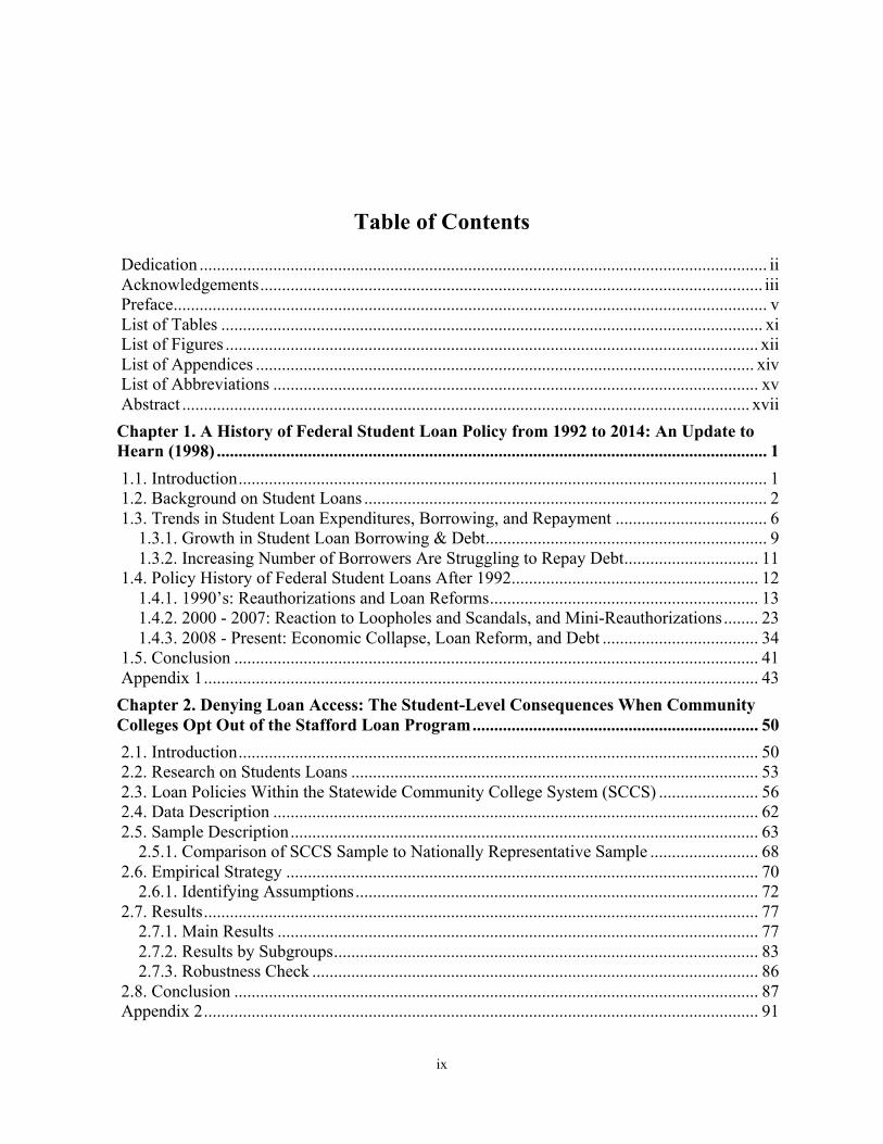
Dedication ................................................................................................................................... ii Acknowledgements .................................................................................................................... iii!Preface ......................................................................................................................................... v!List of Tables ............................................................................................................................. xi!List of Figures ........................................................................................................................... xii!List of Appendices ................................................................................................................... xiv!List of Abbreviations ................................................................................................................ xv!Abstract ................................................................................................................................... xvii!Chapter 1. A History of Federal Student Loan Policy from 1992 to 2014: An Update to Hearn (1998) ............................................................................................................................... 1!1.1. Introduction .......................................................................................................................... 1!1.2. Background on Student Loans ............................................................................................. 2!1.3. Trends in Student Loan Expenditures, Borrowing, and Repayment ................................... 6!
1.3.1. Growth in Student Loan Borrowing & Debt ................................................................. 9!1.3.2. Increasing Number of Borrowers Are Struggling to Repay Debt ............................... 11!
1.4. Policy History of Federal Student Loans After 1992 ......................................................... 12!1.4.1. 1990’s: Reauthorizations and Loan Reforms .............................................................. 13!1.4.2. 2000 - 2007: Reaction to Loopholes and Scandals, and Mini-Reauthorizations ........ 23!1.4.3. 2008 - Present: Economic Collapse, Loan Reform, and Debt .................................... 34!
1.5. Conclusion ......................................................................................................................... 41!Appendix 1 ................................................................................................................................ 43!Chapter 2. Denying Loan Access: The Student-Level Consequences When Community Colleges Opt Out of the Stafford Loan Program .................................................................. 50!2.1. Introduction ........................................................................................................................ 50!2.2. Research on Students Loans .............................................................................................. 53!2.3. Loan Policies Within the Statewide Community College System (SCCS) ....................... 56!2.4. Data Description ................................................................................................................ 62!2.5. Sample Description ............................................................................................................ 63!
2.5.1. Comparison of SCCS Sample to Nationally Representative Sample ......................... 68!2.6. Empirical Strategy ............................................................................................................. 70!
2.6.1. Identifying Assumptions ............................................................................................. 72!2.7. Results ................................................................................................................................ 77!
2.7.1. Main Results ............................................................................................................... 77!2.7.2. Results by Subgroups .................................................................................................. 83!2.7.3. Robustness Check ....................................................................................................... 86!
2.8. Conclusion ......................................................................................................................... 87!Appendix 2 ................................................................................................................................ 91!
x
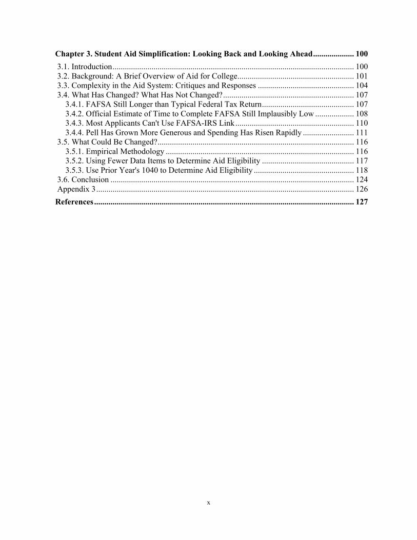
Chapter 3. Student Aid Simplification: Looking Back and Looking Ahead .................... 100!3.1. Introduction ...................................................................................................................... 100!3.2. Background: A Brief Overview of Aid for College ......................................................... 101!3.3. Complexity in the Aid System: Critiques and Responses ............................................... 104!3.4. What Has Changed? What Has Not Changed? ................................................................ 107!
3.4.1. FAFSA Still Longer than Typical Federal Tax Return ............................................. 107!3.4.2. Official Estimate of Time to Complete FAFSA Still Implausibly Low ................... 108!3.4.3. Most Applicants Can't Use FAFSA-IRS Link .......................................................... 110!3.4.4. Pell Has Grown More Generous and Spending Has Risen Rapidly ......................... 111!
3.5. What Could Be Changed? ................................................................................................ 116!3.5.1. Empirical Methodology ............................................................................................ 116!3.5.2. Using Fewer Data Items to Determine Aid Eligibility ............................................. 117!3.5.3. Use Prior Year's 1040 to Determine Aid Eligibility ................................................. 118!
3.6. Conclusion ....................................................................................................................... 124!Appendix 3 .............................................................................................................................. 126!References ............................................................................................................................... 127!

xi
List of Tables Table 1.1. Federal Stafford Loan Limits ......................................................................................... 4!
Table 1.2. Financial Aid Funding for Undergraduate Students ...................................................... 7!
Table 1.3. Share and Average Annual Amount of Undergraduate Borrowing ............................... 9!
Table 1.4. Student Loan Debt for Baccalaureate Graduates ......................................................... 11!
Table 1.5. Repayment Plans for Outstanding Stafford Loans ...................................................... 45!
Table 1.6. Description of Federal Aid Programs .......................................................................... 46!
Table 2.1. Summary Statistics of SCCS Students ......................................................................... 65!
Table 2.2. Comparison of SCCS Students to National Sample of Students ................................. 69!
Table 2.3. Differences in Pre-College Variables by Loan Access ................................................ 74!
Table 2.4. Reduced Form Estimates - Effect of Participating in the Federal Loan Program on Financial Aid & Employment ............................................................................................... 78
Table 2.5. IV Estimates - Effect of Loan Borrowing on Enrollment Intensity ............................. 81!
Table 2.6. IV Estimates - Effect of Loan Borrowing on College Completion ............................. 83!
Table 2.7. Effects of Participating in the Federal Loan Program & Borrowing, by Subgroups ... 84!
Table 2.8. Robustness Check ........................................................................................................ 87!
Table 3.1. Complexity of IRS Tax Forms versus FAFSA .......................................................... 108!
Table 3.2. How Aid Formula Changes Have Affected Pell Grant Targeting ............................. 113!
Table 3.3. Effect of Aid Formula Simplification on Distribution of Pell ................................... 119!
Table 3.4. How Does Using Older Income Data Affect Pell Eligibility? ................................... 122!
xii
List of Figures Figure 1.1. Interest Rate for Stafford and PLUS Loans .................................................................. 5!
Figure 1.2. Federal Grants and Loans as a Share of Total Federal Aid .......................................... 8!
Figure 1.3. National Cohort Default Rate ..................................................................................... 12!
Figure 1.4. New Consolidation Loan Volume .............................................................................. 25!
Figure 1.5. Outstanding Total Debt in the United States .............................................................. 35!
Figure 1.6. Comparison of Loan Forgiveness and Conditional Grant/Loan Programs ................ 49!
Figure 2.1. Number of Stafford Loan Disbursements ................................................................... 57!
Figure 2.2. Share of First-Time Students Borrowing, by School's Loan Participation ................ 57!
Figure 2.3. Cohort Default Rate for the 15 Community Colleges ................................................ 59!
Figure 2.4. Share of Pell-Eligible Students Borrowing Federal or Non-Federal Loans ............... 67!
Figure 2.5. Unemployment Rate ................................................................................................... 95!
Figure 2.6. Share of SCCS Students Receiving Financial Aid ..................................................... 95!
Figure 2.7. Share of Students Transferring in 1st and 2nd Years of Enrollment .......................... 98!
Figure 2.8. Map of SCCS Colleges, by School's Loan Participation ............................................ 98!
Figure 2.9. Share of Students Attending College in Neighboring County or Far Distance .......... 99!
Figure 2.10. First-Time, First Year Enrollment Rates .................................................................. 99!
Figure 3.1. Month of FAFSA Submission for 2007-08 Applicants ............................................ 111!
Figure 3.2. Pell Enrollment and Expenditures Relative to 1976-1977 Levels ............................ 112!
Figure 3.3. Increasing Generosity of the Pell Grant, by Year and Income ................................. 115!
Figure 3.4. Increases in Generosity of the Pell Grant from 2007-08 to 2011-12, by Income .... 115!
xiii
Figure 3.5. Effect of Using Only IRS Data to Define Pell Eligibility: 2007-08 Aid Year ......... 119!
Figure 3.6. Keep Current Formula, Allow All Applicants to Use IRS-FAFSA Link ................. 123!
Figure 3.7. Eliminate FAFSA, Use Older Tax Data to Compute Pell Eligibility ....................... 123!
xiv
List of Appendices Appendix 1.A. Who can Borrow a Stafford Loans? ..................................................................... 43!
Appendix 1.B. Federal Loan Repayment Plans ............................................................................ 44!
Appendix 1.C. Federal Support for Financial Aid ........................................................................ 46!
Appendix 1.D. Description of Loan Forgiveness and Conditional Grant/Loan Programs ........... 47!
Appendix 2.A. Theoretical Framework ........................................................................................ 91!
Appendix 2.B. Supporting Figures for SCCS Loan Participation ................................................ 95!
Appendix 2.C. Additional Identifying Assumptions .................................................................... 96!
Appendix 2.D. Supporting Figures for Identifying Assumptions ................................................. 98!
Appendix 3.A. Data Description ................................................................................................. 126!
xv
List of Abbreviations ACG – Academic Competitiveness Grant AOTC – American Opportunity Tax Credit BAPCA – Bankruptcy Abuse Prevention and Consumer Act of 2005 BEOG – Basic Educational Opportunity Grant BLS – Bureau of Labor Statistics BPS – Beginning Postsecondary Student Study BSLCA – Bipartisan Student Loan Certainty Act of 2013 CAOA - College Access and Opportunity Act CBO – Congressional Budget Office CCRC – College Cost Reduction Act of 2007 CDR – Cohort Default Rate COA – Cost of Attendance CPI – Consumer Price Index CSS – College Scholarship Service DL – Direct Loan Program DRA – Deficit Reduction Act of 2005 ED – U.S. Department of Education ECASLA – Ensuring Continued Access to Student Loans Act of 2008 EFC – Expected Family Contribution FAFSA – Free Application for Federal Student Aid FFEL or FFELP – Federal Family Education Loan Program GAO – General Accountability Office HEA – Higher Education Act HELP – U.S. Senate Committee on Health, Education, Labor, and Pensions HEOA – Higher Education Opportunity Act of 2008 IHEP – Institute for Higher Education Policy IPEDS – Integrated Postsecondary Education Data System IRS – Internal Revenue Service IV – Instrumental Variable LEAP – Leveraging Educational Assistance Partnership LLC – Lifetime Learning Credit NPSAS – National Postsecondary Student Aid Survey NSC – National Student Clearinghouse OLS – Ordinary Least Squares PLUS – Parental Loans for Undergraduate Student SCCS – State Community College System SEOG – Supplemental Educational Opportunity Grant SLS – Supplemental Loans for Students SMART – Science and Mathematics to Retain Tale
xvi
STEM – Science, Technology, Mathematics, and Engineering SSIG – State Student Incentive Grant TEACH – Teacher Education Assistance for College and Higher Education TICAS – The Institute for College Access & Success UI –Unemployment Insurance !
xvii
Abstract
This dissertation examines three different aspects of financial aid policy in the United
States. The first essay describes the evolution of federal student loan policies from 1992 to 2014.
Over time, the federal government’s support for higher education has evolved financial aid from
being grant-based to a student loan centric system. In the early 1970’s, student loans accounted
for less than half of federal expenditures. Today, student loans represent almost two-thirds. In
1998, James Hearn published a book chapter describing the history of federal student loan policy
to establish context for the emergence of student loan use. Since the publication of Hearn’s
chapter, the policies of surrounding student loans and financial aid have changed dramatically. In
this chapter, I trace the history of federal student loan policies from the last two decades and
highlight the political and economic issues that motivated those policy changes, and how the
legacy of those changes shape current financial aid policy.
In the second essay, I investigate the student-level impacts associated with the decision of
community colleges to opt out of the Stafford loan program. The degree to which students are
able to make adequate repayments on their student loans and avoid default is of special concern
for colleges. If too many former students go into default, the college will face sanctions by the
federal government and lose eligibility to provide currently enrolled students federal financial
aid, such as the Pell grant. To avoid these sanctions, some colleges have chosen not to participate
in federal loan programs by excluding loans from students’ financial aid packages. In this
chapter, I investigate the student-level impacts associated with the decision of community
colleges to opt out of the Stafford loan program. Utilizing administrative records from over 50
xviii
community college located in a single state, I estimate the within college differences in outcomes
for Pell-eligible students before and after an institution opts out of the federal loan program. I
find that Pell-eligible students enrolling when the community college offered federal loans are
7.6 percentage points more likely to borrow than Pell-eligible students who enrolled when the
institutions opted out. Overall borrowing also increases by $386 a year. I also find that students
borrowing a loan attempted 19 additional credits in their first year of enrollment and were more
likely to attempt and complete math and science courses than non-borrowers.
The final essay, co-authored with Susan Dynarski, provides a five-year retrospective of
what has changed in the aid application process, what has not, and the possibilities for reform.
Each year, fourteen million households seeking federal aid for college complete a detailed
questionnaire about their finances, the Free Application for Federal Student Aid (FAFSA). At
116 questions, the FAFSA is almost as long as IRS Form 1040 and substantially longer than
Forms 1040EZ and 1040A. Aid for college is intended to increase college attendance by
reducing its price and loosening liquidity constraints. Economic theory, empirical evidence and
common sense suggest that complexity in aid could undermine its ability to affect schooling
decisions. Using data from the nationally representative 2007-08 National Postsecondary Student
Aid Survey (NPSAS), we examine how the distribution of aid would change if applicants could
use older tax information. For example, a student applying in early 2012 for aid for 2012-13
could use IRS data from tax year 2010, rather than 2011. We find that using “prior-prior” tax
information has little effect on aid eligibility, with 65 percent of applicants seeing zero change in
their Pell eligibility and 75 percent seeing a change of less than $500.
1
Chapter 1. A History of Federal Student Loan Policy from 1992 to 2014: An Update to Hearn (1998)
1.1. Introduction In recent years, student loans have received significant attention in both popular media
and policy discourses. Outstanding student loan debt in the United States now exceeds $1
trillion. Media outlets feature stories about individuals who graduated from college with
exceedingly high debt, and then suggest that the “student loan bubble” will follow a similar path
to the housing bubble that occurred in the mid- to late-2000s. Indeed, the share of students
utilizing student loans to finance their college education has substantially increased over the past
several decades. Between 1995-96 and 2011-12, the share of undergraduates borrowing a loan
increased from 26 percent to 42 percent, with the average loan amount growing from $5,655 to
$7,223 (adjusted for inflation) (National Center for Education Statistics, 2015). Today, almost
two-thirds of students are graduating from college with an average debt load greater than
$28,000 (The Institute for College Access & Success, 2014b).
Existing research offers several explanations for the increasing share of students
borrowing and the resulting debt. The first explanation deals with escalating college tuition
prices and the inability of need-based grants to keep pace (Callan, 2001; Hearn & Holdsworth,
2004). Another explanation points to the increase in college enrollment rates, with a larger share
of students having fewer financial resources to pay for college and taking a longer time to
graduate (Baum, 2015; Institute of Education Statistics, 2012) . The third explanation highlights

2
federal financial aid policy, and how current policies are structured to encourage student loan
borrowing (Best & Best, 2014; Mettler, 2014; Mumper, 1996).
In 1998, James Hearn published a book chapter that examined the history of federal
student loan policy to establish the context for the emergence of student loan use. Hearn outlined
student loan policies from the inception of the federal loan program to the early 1990s. Yet, since
the publication of Hearn’s chapter, federal financial aid policies have changed dramatically.
Some of these changes include the introduction of new federal financial aid programs and tax
credits, increases in student loan limits, and alterations to interest rates.
In this paper, I extend Hearn’s work by tracing the history of student loan policy from
1992 to the present and highlighting the political and economic forces that motivated the policy
changes. In his chapter, Hearn stated that it was important to review and understand the history
of federal loan policy in order to illuminate “why particular paths were taken and how the legacy
of taking those paths shapes contemporary policies” (p. 47). Given the significant growth in
student loan borrowing over the past two decades, these words are no less true today.
This paper is structured as follows. In Section 1.2, I describe the types of loans that
students can borrow. Section 1.3 provides an overview of financial aid programs, highlights the
growth in student loan expenditures, and discusses the trends in student loan borrowing. Section
1.4 profiles federal student loan policy from 1992 to 2014. In Section 1.5, I offer concluding
thoughts on the factors contributing to student loan use and the issues that have lead to a national
outstanding student loan debt of over $1 trillion.
1.2. Background on Student Loans Before discussing student loan trends, it is important to specify the types of loans
available to students. In general, federal student loans are offered through three different
3
programs - Perkins, Stafford, and Parental Loans for Undergraduate Students (PLUS).1 Perkins,
the first federal loan program, was created through the National Defense Education Act of 1958.2
Perkins loans are campus-based, wherein the federal government provides institutions with the
capital to lend low-interest loans directly to students. Colleges can collect on the loan and then
re-lend the money to another student. Perkins loans are subsidized, meaning the federal
government pays the interest on the loan while the student is enrolled in college. The current
interest rate is 5 percent and the annual loan limit is $5,500.
The Stafford loan program was created through the Higher Education Act of 1965, which
was a part of President Johnson’s War on Poverty.3 From 1993 to 2010, Stafford loans were
provided to students either directly by the federal government (called the William D. Ford Direct
Loan Program) or through private banks and lenders that received subsidy guarantees from the
federal government (called the Federal Family Education Loan Program or FFEL). With Stafford
loans, students can borrow a subsidized or unsubsidized loan. Like Perkins loans, the federal
government pays the interest on subsidized Stafford loans while the borrower is in school. With
unsubsidized Stafford loans, the interest rate begins accruing when the funds are disbursed to the
student. Prior to 1992, unsubsidized loans were provided only to independent students through
the Supplemental Loans for Students (SLS), which was created as part of the 1986
Reauthorization of the Higher Education Act. Unsubsidized loans replaced SLS during the 1992
Reauthorization and allowed any student to borrow, regardless of income or dependency status.
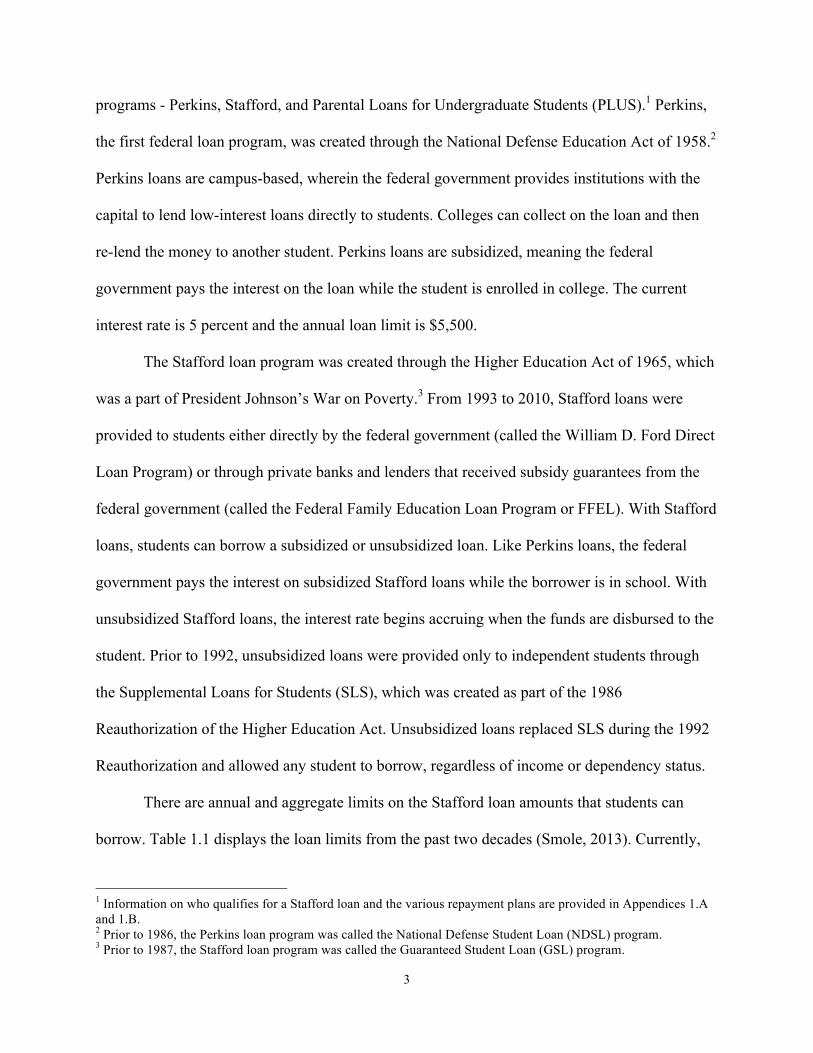
There are annual and aggregate limits on the Stafford loan amounts that students can
borrow. Table 1.1 displays the loan limits from the past two decades (Smole, 2013). Currently,
1 Information on who qualifies for a Stafford loan and the various repayment plans are provided in Appendices 1.A and 1.B. 2 Prior to 1986, the Perkins loan program was called the National Defense Student Loan (NDSL) program. 3 Prior to 1987, the Stafford loan program was called the Guaranteed Student Loan (GSL) program.
4
the subsidized loan limit is $3,500 for the first year, $4,500 for the second year, and $5,500 for
subsequent years. The annual limit (total subsidized and unsubsidized) varies by dependency
status. For example the first year annual loan limit for dependent students is $5,500 and $9,500
for independents. The aggregate loan limit also varies by dependency status. The total amount
students can borrow is $31,000 for dependents and $57,500 for independents.
Table 1.1. Federal Stafford Loan Limits Dependent Students Independent Students Subsidized
Stafford Total Subsidized &
Unsubsidized Stafford Subsidized
Stafford Total Subsidized &
Unsubsidized Stafford Jan. 1987 – Sept. 1992 1st year 2,625 n/a 2,625 6,625 2nd year 2,625 n/a 2,625 6,625 3rd year and beyond 4,000 n/a 4,000 8,000 Aggregate Limit 17,250 n/a 17,250 37,250 Oct. 1992 – June 2007 1st year 2,625 2,625 2,625 6,625 2nd year 3,500 3,500 3,500 7,500 3rd year and beyond 5,500 5,500 5,500 10,500 Aggregate Limit 23,000 23,00 23,000 46,000 July 2007 – June 2008 1st year 3,500 3,500 3,500 7,500 2nd year 4,500 4,500 4,500 8,500 3rd year and beyond 5,500 5,500 5,500 10,500 Aggregate Limit 23,000 23,000 23,000 46,000 July 2008 – current 1st year 3,500 5,500 3,500 9,500 2nd year 4,500 6,500 4,500 10,500 3rd year and beyond 5,500 7,500 5,500 12,500 Aggregate Limit 23,000 31,000 23,000 57,500 Note: Table displays the annual and aggregate loan limits for Stafford Loans. The aggregate limit on total subsidized and unsubsidized loans for independent students also includes SLS loan limits that were available until Oct. 1992. Source: Smole (2013)
The PLUS loan program, created though the 1980 Reauthorization of the Higher
Education Act, allows parents to borrow a loan to help pay for their child’s postsecondary
5
education. Unlike Stafford loans, PLUS loans require a credit check.4 Payments on PLUS loans
begin immediately, but parents do have access to various deferments and forbearances to delay
repayment.
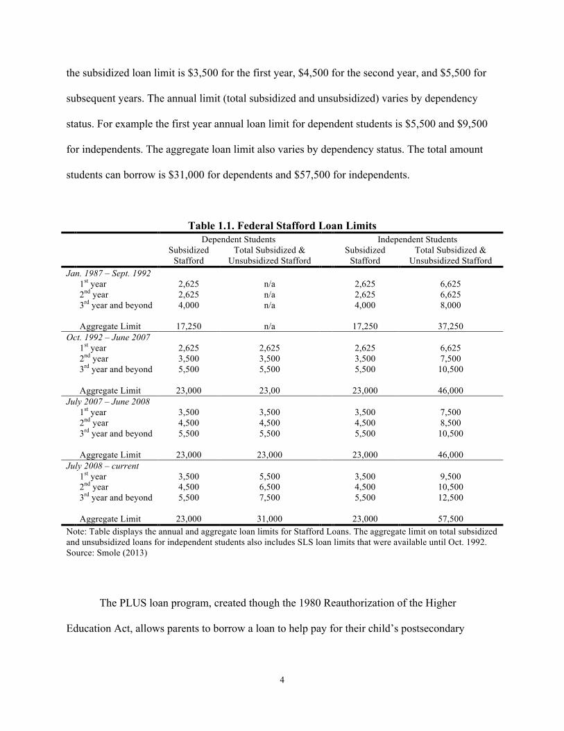
Federal statute establishes the interest rates for Stafford and PLUS loans. Figure 1.1
displays the interest rates from 1992 to 2015 (Smole, 2013). Later I will discuss how the interest
rate formula changed numerous times over the past two decades. In short, the interest rate was
variable from 1992 to 2006 and was calculated based on the bond equivalent rate of the 91-day
Treasury bill plus a premium. All Stafford and PLUS loans disbursed after July 1, 2006 are fixed
interest rate loans.
Figure 1.1. Interest Rate for Stafford and PLUS Loans
Note: Figure displays the in-repayment interest rate for subsidized and unsubsidized loans. From 1995-2006, the in-school interest rate was approximately .6 percentage points lower than the in-repayment interest rate. The interest rate for PLUS after 2006 is for the Direct PLUS loan program. From 2006 to 2010, the FFEL PLUS interest rate was fixed at 8.5 percent. Source: Smole (2013)
4 In the case of a parent having an adverse credit history and is unable to borrow a PLUS loan, the dependent student has the opportunity to borrow at the same annual loan limit (total subsidized and unsubsidized) as an independent student.
0
1
2
3
4
5
6
7
8
9
10
Inte
rest
Rat
e (%
)
1992
-93
1993
-94
1994
-95
1995
-96
1996
-97
1997
-98
1998
-99
1999
-00
2000
-01
2001
-02
2002
-03
2003
-04
2004
-05
2005
-06
2006
-07
2007
-08
2008
-09
2009
-10
2010
-11
2011
-12
2012
-13
2013
-14
2014
-15
Interest Rate Period (July 1 to June 30)
Subsidized & Unsubsidized SubsidizedUnsubsidized PLUS
6
Some students borrow private loans not backed by the federal government. Many states,
employers, and postsecondary institutions offer students loans with terms and interest rates on
par with federal loans. However, educational loans provided by private banks typically represent
the bulk of non-federal loans (College Board, 2014b). These private loans require a credit check
or co-signer with terms that can vary, and interest rates are traditionally higher than the Stafford
loan interest rates. Also, private loans do not provide borrowers the same flexible repayment and
forbearance options available for federal loans. The amount of private loans a student can borrow
is often limited to the cost of attendance, but some banks may allow loan amounts to cover
expenses that are not calculated in the cost of attendance (McSwain, Price, & Cunningham,
2006).5
1.3. Trends in Student Loan Expenditures, Borrowing, and Repayment In addition to student loans, federal support for financial aid is offered through grants,
work-study, veterans and military benefits, and education tax credits.6 Financial aid is also
provided through various state, institutional, and employer supported programs. Table 1.2
displays the programs that have subsidized college costs for college undergraduates over the past
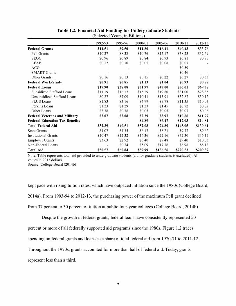
two decades (College Board, 2014b). For the 1992-93 academic year, the total amount of
financial aid awarded to college undergraduates was roughly $51 billion, $32 billion of which
came from the federal government. Two decades later, the total amount increased four-fold to
$209 billion, with the federal government contributing $131 billion.
The more recent growth in financial aid has been largely attributed to the spending
increases in the Pell grant. As Table 1.2 illustrates, Pell expenditures more than doubled between
2005-06 and 2010-11. Despite its funding increase, however, the Pell grant maximum has not 5 Cost of attendance is the tuition and fees that institutions charge students as well as other expenses related to obtaining a higher education. These expenses could include room and board, books, and transportation. 6 More information on these federal aid programs is provided in Appendix 1.C.
7
Table 1.2. Financial Aid Funding for Undergraduate Students (Selected Years, in Billions)
1992-93 1995-96 2000-01 2005-06 2010-11 2012-13
Federal Grants $11.51 $9.50 $11.80 $16.41 $40.43 $33.76
Pell Grants $10.27 $8.38 $10.76 $15.17 $38.23 $32.69
SEOG $0.96 $0.89 $0.84 $0.93 $0.81 $0.75
LEAP $0.12 $0.10 $0.05 $0.08 $0.07 -
ACG - - - - $0.59 -
SMART Grants - - - - $0.46 -
Other Grants $0.16 $0.13 $0.15 $0.22 $0.27 $0.33
Federal Work-Study $0.91 $0.85 $1.13 $1.04 $0.93 $0.88 Federal Loans $17.90 $28.08 $31.97 $47.00 $76.01 $69.38
Subsidized Stafford Loans $11.19 $16.17 $15.29 $19.80 $31.00 $28.35
Unsubsidized Stafford Loans $0.27 $7.09 $10.41 $15.91 $32.87 $30.12
PLUS Loans $1.83 $3.16 $4.99 $9.78 $11.35 $10.03
Perkins Loans $1.23 $1.29 $1.23 $1.45 $0.72 $0.82
Other Loans $3.38 $0.38 $0.05 $0.05 $0.07 $0.06
Federal Veterans and Military $2.07 $2.08 $2.29 $3.97 $10.66 $11.77 Federal Education Tax Benefits - - $4.89 $6.47 $17.03 $14.81 Total Federal Aid $32.39 $40.51 $52.08 $74.89 $145.05 $130.61 State Grants $4.07 $4.35 $6.17 $8.21 $9.77 $9.62 Institutional Grants $10.47 $12.32 $16.36 $22.16 $32.30 $36.17 Employer Grants $3.63 $2.92 $5.40 $7.48 $9.40 $10.03 Non-Federal Loans - $0.74 $5.09 $17.36 $6.98 $8.13 Total Aid $50.57 $60.84 $89.99 $136.56 $220.53 $209.37 Note: Table represents total aid provided to undergraduate students (aid for graduate students is excluded). All values in 2013 dollars. Source: College Board (2014b) kept pace with rising tuition rates, which have outpaced inflation since the 1980s (College Board,
2014a). From 1993-94 to 2012-13, the purchasing power of the maximum Pell grant declined
from 37 percent to 30 percent of tuition at public four-year colleges (College Board, 2014b).
Despite the growth in federal grants, federal loans have consistently represented 50
percent or more of all federally supported aid programs since the 1980s. Figure 1.2 traces
spending on federal grants and loans as a share of total federal aid from 1970-71 to 2011-12.
Throughout the 1970s, grants accounted for more than half of federal aid. Today, grants
represent less than a third.

8
Figure 1.2. Federal Grants and Loans as a Share of Total Federal Aid
Source: College Board (2014b)
From 1992-93 to 2011-12, federal support for loans has increased four-fold from $18
billion to $69 billion (see Table 1.2). Significant growth occurred with the introduction of
unsubsidized loans in 1992. Unsubsidized loans represented less than 2 percent of all federal
loans in 1992-93; by 2012-13, 43 percent of federal loans were unsubsidized. Parental Loans for
Undergraduate Students (PLUS) have also increased nearly five fold over the past two decades.
Perkins loans represent a small portion of federal loan programs and the spending on Perkins has
slowly declined. This decline, however, is masked by the significant rise in unsubsidized and
PLUS spending.
Non-federal loans also experienced notable growth in the mid-2000s. By 2005-06, non-
federal sources of aid represented more than 12 percent of all financial aid and, at $17.36 billion,
non-federal loan volume was higher than Pell volume. With the market collapse in 2008 and the
increase in federal loan maximums (which will be discussed later), non-federal loan volume
0
.1
.2
.3
.4
.5
.6
.7
.8
.9
1
Shar
e of
Tot
al F
eder
al A
id
1970
-71
1975
-76
1980
-81
1985
-86
1990
-91
1995
-96
2000
-01
2005
-06
2010
-11
Academic Year
Federal Grants Federal Loans
9
declined to less than $10 billion in 2012-13.
1.3.1. Growth in Student Loan Borrowing & Debt
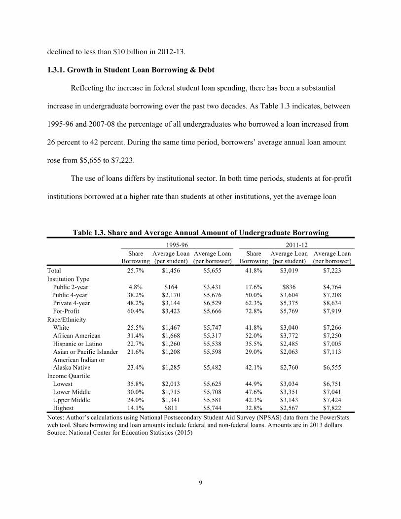
Reflecting the increase in federal student loan spending, there has been a substantial
increase in undergraduate borrowing over the past two decades. As Table 1.3 indicates, between
1995-96 and 2007-08 the percentage of all undergraduates who borrowed a loan increased from
26 percent to 42 percent. During the same time period, borrowers’ average annual loan amount
rose from $5,655 to $7,223.
The use of loans differs by institutional sector. In both time periods, students at for-profit
institutions borrowed at a higher rate than students at other institutions, yet the average loan
Table 1.3. Share and Average Annual Amount of Undergraduate Borrowing 1995-96 2011-12
Share
Borrowing Average Loan (per student)
Average Loan (per borrower) Share
Borrowing Average Loan (per student)
Average Loan (per borrower)
Total 25.7% $1,456 $5,655 41.8% $3,019 $7,223 Institution Type
Public 2-year 4.8% $164 $3,431 17.6% $836 $4,764 Public 4-year 38.2% $2,170 $5,676 50.0% $3,604 $7,208
Private 4-year 48.2% $3,144 $6,529 62.3% $5,375 $8,634 For-Profit 60.4% $3,423 $5,666 72.8% $5,769 $7,919
Race/Ethnicity White 25.5% $1,467 $5,747 41.8% $3,040 $7,266
African American 31.4% $1,668 $5,317 52.0% $3,772 $7,250 Hispanic or Latino 22.7% $1,260 $5,538 35.5% $2,485 $7,005 Asian or Pacific Islander 21.6% $1,208 $5,598 29.0% $2,063 $7,113 American Indian or Alaska Native 23.4% $1,285 $5,482 42.1% $2,760 $6,555
Income Quartile Lowest 35.8% $2,013 $5,625 44.9% $3,034 $6,751
Lower Middle 30.0% $1,715 $5,708 47.6% $3,351 $7,041 Upper Middle 24.0% $1,341 $5,581 42.3% $3,143 $7,424 Highest 14.1% $811 $5,744 32.8% $2,567 $7,822
Notes: Author’s calculations using National Postsecondary Student Aid Survey (NPSAS) data from the PowerStats web tool. Share borrowing and loan amounts include federal and non-federal loans. Amounts are in 2013 dollars. Source: National Center for Education Statistics (2015)

10
amount is consistently higher at private four-year institutions. For all sectors, there has been a
significant increase in the share of students borrowing over time. For example, in 1995-96, 4.8
percent of students at public two-year institutions took out a student loan. This increased to 17.6
percent in 2011-12. The sector with the largest growth is 4-year private institutions—the share of
students borrowing rose 14.1 percentage points (see Table 1.3 for details).
The likelihood of borrowing and the amount of money borrowed also differs by
race/ethnicity and income. While minority and lower income students are more likely to borrow,
the loan amount they borrow is less, on average, than their peers. In both 1995-96 and 2011-12,
African Americans had the highest share of student borrowers. Yet, conditional on borrowing,
Whites had the highest average loan amount in the two time periods. Students in the lowest
quartile of the income distribution had the highest share of students borrowing in 1995-96,
roughly 36 percent. By 2011-12, the income the group with the highest share shifted to the lower
middle quartile; 48 percent of these students took out a loan. Students in the highest quartile had
the lowest share of students borrowing, but, among student loan borrowers, had the largest
average loan amounts at $5,744 in 1995-96 and $7,822 in 2011-12.
The increasing annual share of students borrowing and the rise in loan amounts has led to
a significant increase in students graduating with debt. As Table 1.4 displays, the share of
baccalaureate recipients with debt increased from 55 percent in 1992-93 to 71 percent in 2011-12
(Hershbein & Hollenbeck, 2014; 2015; as cited in Lochner & Monge-Naranjo, 2015). The
average cumulative loan debt per graduate also grew three times larger from $7,300 to $21,200.
When the sample is restricted to those graduates who borrowed, the average loan debt more than
doubled from $13,200 to $29,700.

11
Table 1.4. Student Loan Debt for Baccalaureate Graduates
Average Loan Average Loan
Year Graduating Share Borrowing (per graduate) (per borrower) 1990 54.5% $7,200 $13,200 1996 52.6% $9,200 $17,600 2000 63.6% $14,400 $22,600 2004 65.6% $14,800 $22,600 2008 68.2% $17,200 $25,200 2012 71.0% $21,220 $29,700 Notes: Table adapted from Lochner and Monge-Naranjo (2015). Amounts are in 2013 dollars. Share borrowing and loan amounts include federal and non-federal loans. Source: Hershbein and Hollenbeck (2014, 2015)
1.3.2. Increasing Number of Borrowers Are Struggling to Repay Debt
As both the percentage of students who borrow and the average loan debt with which
students graduate have increased, the consequences of a financial aid system increasingly
predicated on loans are becoming apparent. Troublingly, research suggests that a significant
number of individuals are struggling to repay their student loans. In 2014, nearly 11 percent of
student debt was 90 days delinquent or in default (Federal Reserve Bank of New York, 2015).
Estimates of delinquency or default rates are even larger for particular cohorts. Of the students
who entered repayment in 2005, for example, nearly 26 percent had become delinquent and 15
percent had defaulted at some point within the first five years of repayment (Cunnhinghum &
Kienzl, 2011).
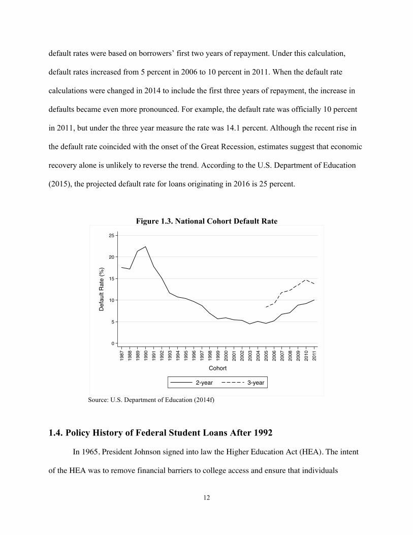
The default rate is commonly used to gauge students’ ability to repay.7 Figure 1.3
displays the official cohort default rates for Stafford loan borrowers. After a slow decline in
default rates between the mid-1990s and the mid-2000s, the default rate started to rise
dramatically in 2007, which coincides with the start of the Great Recession. Prior to 2014,
7 The default rate measure is calculated from the share of borrowers entering repayment and failed to make a loan payment for a certain number of days. Prior to 1985, borrowers were identified as being in default if they had not made a loan payment for more than 120 days. The definition of default changed from 120 days to 180 in 1985, and then to the now current 270 days in 1998.
12
default rates were based on borrowers’ first two years of repayment. Under this calculation,
default rates increased from 5 percent in 2006 to 10 percent in 2011. When the default rate
calculations were changed in 2014 to include the first three years of repayment, the increase in
defaults became even more pronounced. For example, the default rate was officially 10 percent
in 2011, but under the three year measure the rate was 14.1 percent. Although the recent rise in
the default rate coincided with the onset of the Great Recession, estimates suggest that economic
recovery alone is unlikely to reverse the trend. According to the U.S. Department of Education
(2015), the projected default rate for loans originating in 2016 is 25 percent.
Figure 1.3. National Cohort Default Rate
Source: U.S. Department of Education (2014f)
1.4. Policy History of Federal Student Loans After 1992 In 1965, President Johnson signed into law the Higher Education Act (HEA). The intent
of the HEA was to remove financial barriers to college access and ensure that individuals
0
5
10
15
20
25
Def
ault
Rat
e (%
)
1987
1988
1989
1990
1991
1992
1993
1994
1995
1996
1997
1998
1999
2000
2001
2002
2003
2004
2005
2006
2007
2008
2009
2010
2011
Cohort
2-year 3-year
13
wanting to go to college would have financial support from the federal government to do so. To
keep the HEA up to date, Congress periodically amends and reauthorizes provisions within the
bill. Prior to 1992, the HEA was amended and reauthorized in 1972, 1978, 1980, and 1986. Over
time, Congressional action to increase access to higher education with the introduction of new
HEA financial aid programs has significantly expanded the federal government’s role in higher
education. The HEA accounts for over 60 percent of all financial aid available to students, and a
significant portion of this aid is in the form of student loans.
The following section provides a detailed history of federal loan policy over the last two
decades, picking up where Hearn left off by starting with what transpired during the 1992 HEA
Reauthorization. The intent of this section is to highlight what particular federal actions were
taken in relation to student loans and why, and to examine how these actions contributed to the
growth in student loan borrowing and continue to shape current federal financial aid policies.
1.4.1. 1990’s: Reauthorizations and Loan Reforms
In the early 1990s, the financial aid system for postsecondary education in the United
States was facing a myriad of issues that Congress wished to address with the upcoming 1992
Reauthorization of the Higher Education Act (HEA).8 First, the formula determining the amount
of money that families could be expected to contribute to the cost of a student’s education was
confusing and complex. Students completed one form to apply for financial aid, but the
information from the application created two separate Expected Family Contribution (EFC)
amounts - one to be used for the Pell grant program and a second for other forms of federal aid
(Fitzgerald, 2006). In an attempt to reduce the complexity of the application process,
policymakers wanted to create a single EFC that could be used across all federal aid programs
(Schenet, 1993). 8 Throughout this paper, Higher Education Act and HEA will be used interchangeably.
14
Second, the annual cost of attendance (which includes tuition, fees, and room and board)
was increasing at a rate that was outpacing inflation (Schenet, 1993). Need-based grants, such as
the Pell grant, had failed to keep pace with rising tuition rates and were losing their purchasing
power. This meant that the maximum award amount from the Pell grant was not providing
enough resources for low-income students to attend moderately priced institutions. At the same
time, parents were contributing less to their children’s college education than parents from the
previous generation (Fossey, 1998) and, because of aid reforms under the Reagan administration,
there was little federal financial assistance available for middle- and upper-income families
(Hearn, 1998; Mumper, 1996). Policymakers needed to figure out a way to increase the
purchasing power of the Pell grant and expand the eligibility of federal aid programs to middle-
income families.
Third, because of the rising tuition rates and the inability of need-based grants to keep
pace, students were borrowing more loans than they had in the two decades prior and were
graduating with debt that some feared had become unmanageable. The cohort default rate
reached an historic high of 22.4 percent in 1990 (see Figure 1.3). This meant that almost 1 in 4
loans were going into default. The high default rates resulted in significant costs for the federal
government; in 1991, $3.6 billion was spent to cover default claims (U.S. General Accounting
Office, 1995).
Rather than blaming borrowers for the rising default rates, several reports by the U.S.
General Accounting Office (1991, 1992)9 and the Permanent Senate Subcommittee on
Investigations (1991) pointed to for-profit colleges and FFEL lenders as the source of the
problem. These reports noted that borrowers were attending proprietary institutions that did not
provide a quality education and argued that these institutions only existed to take advantage of 9 Now known as the Government Accountability Office.
15
the “cash cow” provided to them by the federal government. Many of these students were
leaving college with little or no training and accumulated loan debt that could not be repaid
because they lacked the skills needed to obtain a job. There was also evidence that proprietary
schools were recruiting low-income students who, for various reasons, were highly unlikely to
ever complete their postsecondary degree. The reports also pointed out that FFEL lenders had
little incentive to help borrowers repay their loans because the loan program posed little to no
risk for lenders. Most notably, the federal government reimbursed lenders for defaulted loans.
The aforementioned issues surrounding student loans made the program costly for the
federal government, and it became evident that the whole loan program was in shambles. Senator
Edward Kennedy argued that “the student loan program may be just one step ahead of disaster”
(cited in Mumper, 1996, p. 100). The Permanent Senate Subcommittee on Investigations (1991)
was more direct: they noted that the loan program was “plagued by fraud and abuse at every
level and lacking meaningful oversight and management controls, the program has become
inefficient, ineffective, and far too costly” (p. 33).
1.4.1.1. 1992 Reauthorization of the Higher Education Act Addressing all the issues described above in one broad piece of legislation would be a
difficult task, given the political climate at the time. Politicians had the desire to expand
eligibility and increase the benefits of federal aid programs, yet Presidential and congressional
elections were approaching, and President George H. W. Bush was determined to cut back on
federal spending (Mumper, 1996). This meant a possible Presidential veto loomed over any
effort to increase the scope of financial aid, and the threat of a veto influenced the issues that
would be addressed in the final bill. For example, because of this political climate, one important
16
proposal – to make the Pell grant program an entitlement and increase the maximum award
amount – was abandoned.
In spite of the limitations necessitated by the political climate, the passage of the 1992
Reauthorization ushered in the largest reform in federal financial aid since the 1970s (Mumper,
1996). While the bill did not constitute the reform that many individuals felt was needed, it did
provide a significant framework for financial aid that is still used today. The provisions within
the bill altered the calculation used to determine students’ financial need, provided aid access to
middle-income families, introduced new flexible student loan repayment options, and created
more government oversight of for-profit institutions.
In order to simplify and improve the process of determining aid eligibility,
Reauthorization developed a single method for calculating students’ financial need, and created a
new application – still in use today – known as the Free Application for Federal Student Aid
(FAFSA) (Fitzgerald, 2006). The new aid application and formula no longer considered home
and family farm equities as available assets and ignored all financial assets for families with
income below $50,000 and receiving means-tested federal benefits. Compared to the old need
analysis formula, the new formula expanded eligibility for federal aid programs, particularly
loans.
Reauthorization also addressed the concerns of middle-income families hit particularly
hard by the rising cost of college attendance. Middle-income students benefited from the creation
of the Stafford unsubsidized loan program, which provided federal loan access to all students
regardless of their families’ financial need or income. Additionally, the annual loan limits under
the Stafford loan program increased for second-year undergraduates from $2,625 to $3,500, and
the maximum for upper division undergraduates increased from $4,000 to $5,500 (see Table

17
1.1). The aggregate loan amount limit increased from $17,250 to $23,000 for dependent students,
and $37,250 to $46,000 for independent students. Parents benefited from the changes to the
PLUS loan program that allowed them to borrow larger loan amounts. Prior to 1992, the amount
of money parents could borrow through the PLUS loan program was capped at $4,000.
Reauthorization eliminated this cap and allowed parent to receive a PLUS loan up to the cost of
attendance minus any aid the student received.
In an attempt to curb the high default rate, the 1992 Reauthorization introduced new debt
relief and flexible repayment options for borrowers. One provision, for example, encouraged the
Department of Education (ED) to work with employers from the public and private sectors to
provide options that would help borrowers repay federal loans. Suggested mechanisms included
payroll deductions for loan payments and loan repayment matching provisions as part of
employee benefit packages. The bill also required lenders to provide borrowers with graduated or
income sensitive repayment options. Graduated repayment grants borrowers a month payment
amount that increases over time – the borrower makes small payments first and then larger
payments later. This repayment option is structured on the assumption that borrowers’ income
will increase over the repayment period. Similarly, income sensitive repayment provides
borrowers with a monthly payment amount that is annually adjusted to their income. The
Reauthorization bill also increased the amount of time an unemployed borrower can defer
payments from 2 years to 3, and made a new loan deferment available to borrowers who were
facing “economic hardship.” Borrowers could defer payments while receiving public assistance
or working full-time with a monthly income 150% below the federal poverty line.
To halt future abuse and fraud from proprietary institutions, the Reauthorization
amendments enacted new accountability and oversight provisions. One provision was the “85/15
18
rule” (Skinner, 2007), which stipulated that for-profit college could not derive more than 85
percent of their total revenue from federal aid programs. In addition, because many of the for-
profit colleges offered courses through telecommunications or correspondence, a new provision
called the “50% rule” was created. Under this provision, an institution loses federal aid funding
if more than 50 percent of the institution’s courses are offered through telecommunications or
correspondence.
Although not fully implemented by the final bill, the debate and discussion surrounding
the 1992 Reauthorization introduced an idea that would play a key role in future financial aid
policy: the move to end FFEL and lender participation in the federal Stafford loan programs, and
direct all federal student loans through the federal government. Under this new plan, known as
direct lending, student loans are financed entirely with federal capital and are provided directly
to students. Supporters of the program argued that removing private lenders, guarantee agencies,
and secondary markets would save taxpayers billions of dollars. The direct loan program would
also simplify loan delivery and free institutions from having to deal with multiple lenders.
Opponents of direct lending questioned the estimated cost savings and suggested that the current
FFEL program had already proven its effectiveness over time. They argued that the move to a
new system would be nothing more than an untested experiment at the taxpayers’ expense
(Mumper, 1996).
As support for a full-scale move to direct lending was gaining momentum, particularly
among Democrats, Education Secretary Lamar Alexander announced he was opposed to direct
lending, and President Bush threatened to veto the Reauthorization bill if such a program was
created (Mumper, 1996). As a compromise, the direct loan program was codified as a
demonstration project that allowed no more than 300 institutions to participate.

19
1.4.1.2. President Clinton and the Move to Direct Lending When Bill Clinton began his presidential term in 1993, he proposed a streamlined loan
program with a national service component to replace existing federal loan programs (Mumper,
1996). Clinton believed that many college graduates were avoiding public service jobs because
they incurred too much student loan debt (Waldman, 1995), and he suggested a new loan
program consisting of income contingent loans. Under this proposal, borrowers’ monthly
payments would be based on their income and, after a certain period of time, the remaining loan
balance would be forgiven in exchange for public service. The overall idea was to reform student
loans into a streamlined system – one loan program with a flexible repayment option. Cost
estimates of Clinton’s new student loan program were high, upwards of eight billion dollars a
year (Waldman, 1995). The anticipated costs forced Clinton to scale back his national service
proposal. The final version of his plan created the AmeriCorps program, which, at its inception,
provided participants up to $4,750 to repay student loans in exchange for a year of service; the
program was limited to no more than 100,000 people (Hearn, 1998; Waldman, 1995).
President Clinton’s desire to streamline the student loan system provided momentum for
the implementation of the Direct Loan program proposed during the 1992 Reauthorization.
Clinton embraced the program’s projected financial savings and wanted to tie direct loans to an
income-contingent repayment option (Waldman, 1995). This type of repayment option would
determine borrowers’ monthly payment amount—adjusted annually—based on outstanding loan
balance, adjusted gross income, and family size. Borrowers would also have their loans
discharged (or forgiven) after a 25-year repayment period.
While President Clinton and House Democrats favored a full-scale and immediate
implementation of direct lending, Democrats in the Senate, namely Senators Claiborne Pell and
20
Edward Kennedy, proposed that the program be gradually phased-in in order to assess the
program’s effectiveness (Cervantes et al., 2005; Waldman, 1995). Ultimately, direct lending and
income contingent repayment were approved through the passage of the Student Loan Reform
Act of 1993 with a gradual phase-in. The new loan program was called the William D. Ford
Direct Loan Program and the transition to direct lending was to occur over a 5-year period: direct
lending would comprise 5 percent of federal loans in 1994-95, 40 percent in 1995-96, 50 percent
in 1996-97, and 60 percent in 1997-98 and 1998-99. In contrast to the legislative intent, direct
lending’s share of the loan market only peaked to a high of 34 percent in fiscal year 1997
(Cervantes et al., 2005). Postsecondary institutions were hesitant to make the move to direct
lending for fear that the program was not fully tested; they wanted to give the federal
government time to work out any initial problems. Because of this hesitation, the phase-in
provisions were later repealed and institutions continued to have the choice of participating in
either the Direct Loan program or the Federal Family Education Loan program.
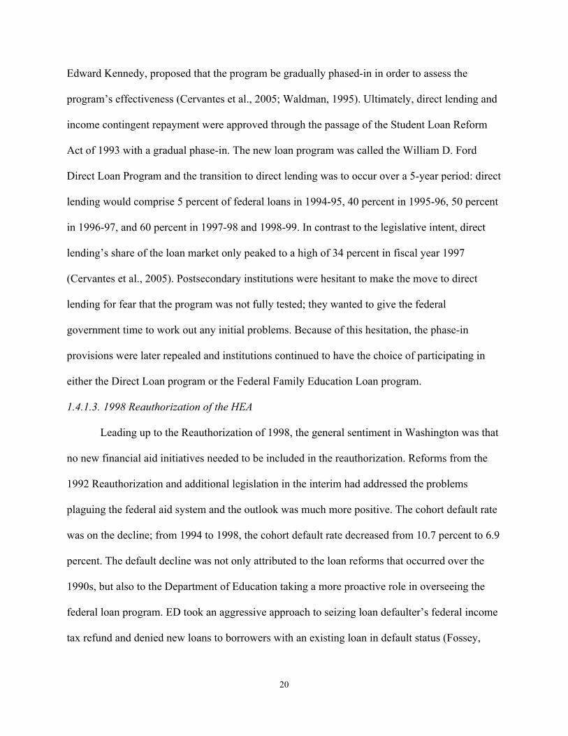
1.4.1.3. 1998 Reauthorization of the HEA
Leading up to the Reauthorization of 1998, the general sentiment in Washington was that
no new financial aid initiatives needed to be included in the reauthorization. Reforms from the
1992 Reauthorization and additional legislation in the interim had addressed the problems
plaguing the federal aid system and the outlook was much more positive. The cohort default rate
was on the decline; from 1994 to 1998, the cohort default rate decreased from 10.7 percent to 6.9
percent. The default decline was not only attributed to the loan reforms that occurred over the
1990s, but also to the Department of Education taking a more proactive role in overseeing the
federal loan program. ED took an aggressive approach to seizing loan defaulter’s federal income
tax refund and denied new loans to borrowers with an existing loan in default status (Fossey,
21
1998). Perhaps most important was a rule created in the late 1980s, wherein the ED targeted
postsecondary institutions with a high default rate and sanctioned them from participating in
federal aid programs, such as the Pell grant.
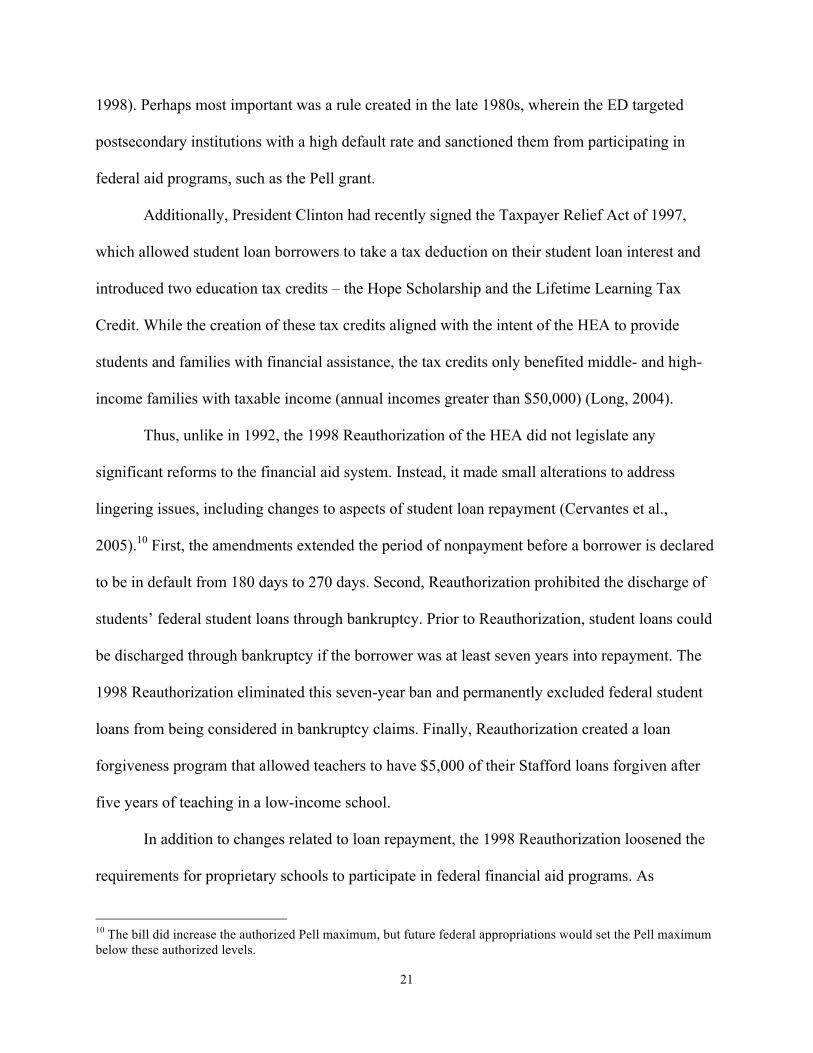
Additionally, President Clinton had recently signed the Taxpayer Relief Act of 1997,
which allowed student loan borrowers to take a tax deduction on their student loan interest and
introduced two education tax credits – the Hope Scholarship and the Lifetime Learning Tax
Credit. While the creation of these tax credits aligned with the intent of the HEA to provide
students and families with financial assistance, the tax credits only benefited middle- and high-
income families with taxable income (annual incomes greater than $50,000) (Long, 2004).
Thus, unlike in 1992, the 1998 Reauthorization of the HEA did not legislate any
significant reforms to the financial aid system. Instead, it made small alterations to address
lingering issues, including changes to aspects of student loan repayment (Cervantes et al.,
2005).10 First, the amendments extended the period of nonpayment before a borrower is declared
to be in default from 180 days to 270 days. Second, Reauthorization prohibited the discharge of
students’ federal student loans through bankruptcy. Prior to Reauthorization, student loans could
be discharged through bankruptcy if the borrower was at least seven years into repayment. The
1998 Reauthorization eliminated this seven-year ban and permanently excluded federal student
loans from being considered in bankruptcy claims. Finally, Reauthorization created a loan
forgiveness program that allowed teachers to have $5,000 of their Stafford loans forgiven after
five years of teaching in a low-income school.
In addition to changes related to loan repayment, the 1998 Reauthorization loosened the
requirements for proprietary schools to participate in federal financial aid programs. As
10 The bill did increase the authorized Pell maximum, but future federal appropriations would set the Pell maximum below these authorized levels.
22
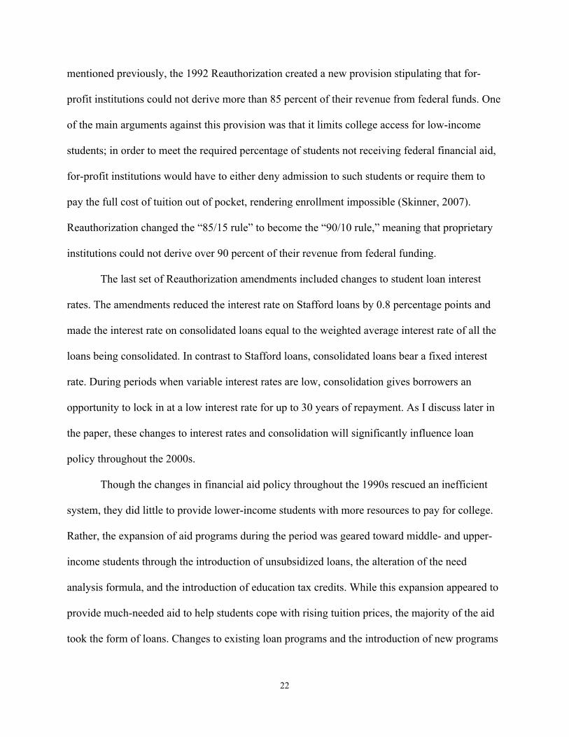
mentioned previously, the 1992 Reauthorization created a new provision stipulating that for-
profit institutions could not derive more than 85 percent of their revenue from federal funds. One
of the main arguments against this provision was that it limits college access for low-income
students; in order to meet the required percentage of students not receiving federal financial aid,
for-profit institutions would have to either deny admission to such students or require them to
pay the full cost of tuition out of pocket, rendering enrollment impossible (Skinner, 2007).
Reauthorization changed the “85/15 rule” to become the “90/10 rule,” meaning that proprietary
institutions could not derive over 90 percent of their revenue from federal funding.
The last set of Reauthorization amendments included changes to student loan interest
rates. The amendments reduced the interest rate on Stafford loans by 0.8 percentage points and
made the interest rate on consolidated loans equal to the weighted average interest rate of all the
loans being consolidated. In contrast to Stafford loans, consolidated loans bear a fixed interest
rate. During periods when variable interest rates are low, consolidation gives borrowers an
opportunity to lock in at a low interest rate for up to 30 years of repayment. As I discuss later in
the paper, these changes to interest rates and consolidation will significantly influence loan
policy throughout the 2000s.
Though the changes in financial aid policy throughout the 1990s rescued an inefficient
system, they did little to provide lower-income students with more resources to pay for college.
Rather, the expansion of aid programs during the period was geared toward middle- and upper-
income students through the introduction of unsubsidized loans, the alteration of the need
analysis formula, and the introduction of education tax credits. While this expansion appeared to
provide much-needed aid to help students cope with rising tuition prices, the majority of the aid
took the form of loans. Changes to existing loan programs and the introduction of new programs
23
generated opportunities for students to take on additional debt (Mumper, 1996). By essentially
equating access to college with access to loans, the policy changes reduced the role of taxpayer
support and began shifting the burden of paying for college squarely onto the shoulders of
students and families (St. John, 2006).
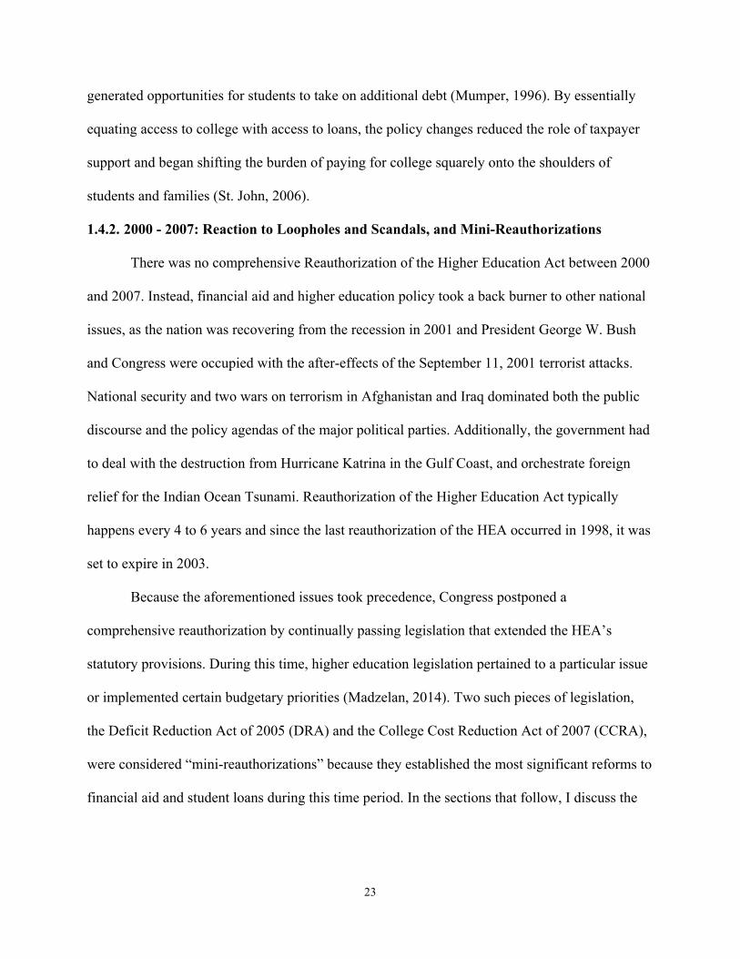
1.4.2. 2000 - 2007: Reaction to Loopholes and Scandals, and Mini-Reauthorizations There was no comprehensive Reauthorization of the Higher Education Act between 2000
and 2007. Instead, financial aid and higher education policy took a back burner to other national
issues, as the nation was recovering from the recession in 2001 and President George W. Bush
and Congress were occupied with the after-effects of the September 11, 2001 terrorist attacks.
National security and two wars on terrorism in Afghanistan and Iraq dominated both the public
discourse and the policy agendas of the major political parties. Additionally, the government had
to deal with the destruction from Hurricane Katrina in the Gulf Coast, and orchestrate foreign
relief for the Indian Ocean Tsunami. Reauthorization of the Higher Education Act typically
happens every 4 to 6 years and since the last reauthorization of the HEA occurred in 1998, it was
set to expire in 2003.
Because the aforementioned issues took precedence, Congress postponed a
comprehensive reauthorization by continually passing legislation that extended the HEA’s
statutory provisions. During this time, higher education legislation pertained to a particular issue
or implemented certain budgetary priorities (Madzelan, 2014). Two such pieces of legislation,
the Deficit Reduction Act of 2005 (DRA) and the College Cost Reduction Act of 2007 (CCRA),
were considered “mini-reauthorizations” because they established the most significant reforms to
financial aid and student loans during this time period. In the sections that follow, I discuss the

24
financial aid issues leading up to the passage of DRA and CCRA and the policy changes enacted
through other legislation before highlighting key provisions of both bills.
1.4.2.1. Student Loan Loopholes
From 2002-03 to 2005-06, the interest rate on federal student loans reached historic lows
(see Figure 1.1). Borrowers already in repayment on variable interest rate loans were
consolidating their loans to take advantage of the low fixed interest rate, especially before 2006
when the variable interest rate was scheduled to increase 2 percentage points. In addition, due to
legislation passed in 2001, the interest rate for students currently enrolled in school was set to
change from variable to a fixed 6.8 percent on July 1, 2006 (Delisle, 2012). While consolidation
was developed to help borrowers in repayment, a loophole in the Higher Education Act made it
possible for students to consolidate their loans while enrolled in school. Enrolled students could
notify their lenders of their wish to enter early repayment, consolidate their loans, and then
request an in-school deferment.11
The upcoming increase in interest rates, combined with the in-school consolidation
loophole, resulted in an explosion in the number of loan consolidations, especially in the FFEL
program. As Figure 1.4 illustrates, the FFEL consolidation volume grew over 600 percent, from
$9.4 billion in 2001 fiscal year to $72 billion in 2006. The U.S. Government Accountability
Office (2004) estimated that the federal government was spending over $1 billion each year in
subsidies to lenders to help with loan consolidations. To reduce consolidation costs, the in-school
consolidation loophole was eliminated in 2005. After 2007, interest rates increased (see Figure
1.1) and changed from variable to fixed, which made consolidation less attractive to students and
accounted for the significant decline in new consolidation volume depicted in Figure 1.4.
11 This loophole was applicable for FFEL loans. Students at Direct loan schools could consolidate their loans while enrolled and in repayment.
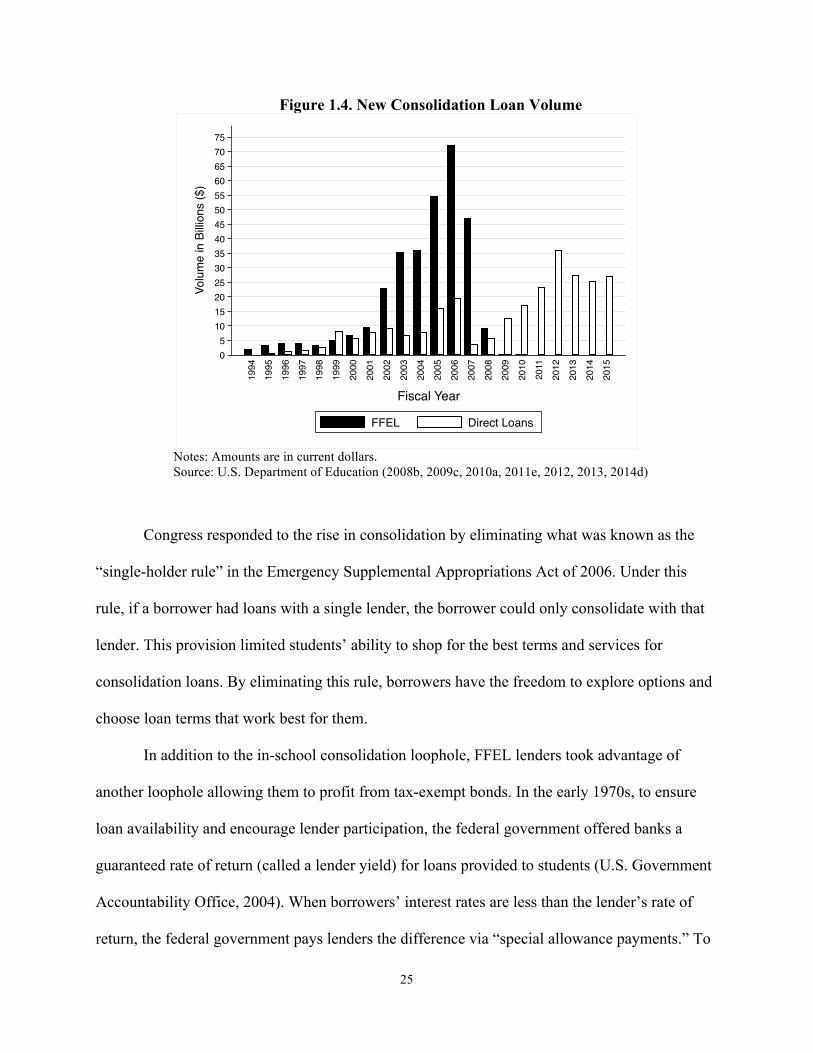
25
Figure 1.4. New Consolidation Loan Volume
Notes: Amounts are in current dollars. Source: U.S. Department of Education (2008b, 2009c, 2010a, 2011e, 2012, 2013, 2014d)
Congress responded to the rise in consolidation by eliminating what was known as the
“single-holder rule” in the Emergency Supplemental Appropriations Act of 2006. Under this
rule, if a borrower had loans with a single lender, the borrower could only consolidate with that
lender. This provision limited students’ ability to shop for the best terms and services for
consolidation loans. By eliminating this rule, borrowers have the freedom to explore options and
choose loan terms that work best for them.
In addition to the in-school consolidation loophole, FFEL lenders took advantage of
another loophole allowing them to profit from tax-exempt bonds. In the early 1970s, to ensure
loan availability and encourage lender participation, the federal government offered banks a
guaranteed rate of return (called a lender yield) for loans provided to students (U.S. Government
Accountability Office, 2004). When borrowers’ interest rates are less than the lender’s rate of
return, the federal government pays lenders the difference via “special allowance payments.” To
05
1015202530354045505560657075
Volu
me
in B
illion
s ($
)
1994
1995
1996
1997
1998
1999
2000
2001
2002
2003
2004
2005
2006
2007
2008
2009
2010
2011
2012
2013
2014
2015
Fiscal Year
FFEL Direct Loans
26
finance loans in the 1970s, the federal government allowed state-designated authorities to sell
tax-exempt bonds and use the proceeds to make loans with a minimum lender yield of 9.5
percent (Kvaal & Shireman, 2004). In 1993, the 9.5 percent lender yield minimum was
eliminated. However, any loans financed with proceeds from the tax-exempt bonds prior to 1993
were still guaranteed a minimum 9.5 percent rate of return. By 2004, it was discovered that the
federal government was still paying FFEL lenders who were issuing loans financed with pre-
1993 tax-exempt bonds. Because the borrower interest rates were extremely low compared to the
9.5 percent guaranteed return, the special allowance payments to FFEL lenders increased
dramatically from $209 million in 2001 to over $634 million in 2004 (U.S. Government
Accountability Office, 2004). Discovering that lenders continued to take advantage of this
loophole at a large cost to taxpayers, Congress passed the Taxpayer-Teacher Protection Act of
2004 and eliminated the 9.5 percent lender yield for all loans financed from tax-exempt bonds,
regardless of when the proceeds were generated. Using the money saved from this provision,
Congress supplemented the 1998 teacher loan forgiveness program by raising the forgiveness
amount to $17,500 for individuals teaching for 5 consecutive years in mathematics, science, or
special education.
1.4.2.2. Student Loan Lender Scandals
Following the recession in 2001, college enrollment rates grew and state funding for
higher education declined (Tandberg, 2010; Toutkoushian & Shafiq, 2010). To generate
additional revenue, an increasing number of colleges began to engage in a practice called “school
as lender.” Colleges would obtain a line of credit from a bank or use their own capital to provide
student loans to graduate students. The college would then sell its loan portfolio to lenders and
use the revenue to create need-based financial aid for undergraduate students. According to a
27
GAO (2005) report, the value of loans originated by school lenders grew from $535 million in
1999-00 to over $1.5 billion in 2003-04.
The GAO report noted several concerns with colleges acting as lenders. First, since
colleges determine both cost of attendance and students’ eligibility for student loans, a conflict of
interest arises because the colleges making loans financially benefit from increases in tuition
rates and the resulting student debt. Second, the report questioned the schools’ contractual
relationships with lenders and whether these relationships created an incentive for the school to
encourage student borrowing. The bargaining practices between colleges and lenders potentially
violated an HEA provision called the “anti-inducement provision.” This provision prohibits “any
lender from offering gifts or other incentives to schools or individuals to secure FFEL
applicants” (GAO, 2005, p. 5). At the time, the Department of Education was not actively
enforcing this provision. In a 2003 memo, the Department of Education’s Office of Inspector
General stated that guidance on inducements and gifts were outdated and urged the Department
to issue new guidelines to clarify what constitutes an inducement. Though the Department of
Education did not take any action in response to the memo, Congress eliminated the ability for
colleges to act as a lender in 2005.
Abolishing the school as lender practice did not quell all concerns about the relationships
between lenders and colleges. In 2006, New York Attorney General Andrew Cuomo announced
he would begin an investigation into the lending practices of the student loan industry. At the
conclusion of his investigation in 2007, Cuomo revealed numerous scandals in which student
loan lenders were providing financial compensation to schools with the expectation that the
lender will be placed on the college’s “preferred lender” list (New York State Office of the
Attorney General, 2007). It was also discovered that lenders were giving financial aid
28
administrators all-expenses-paid trips to high-end resorts and paid positions on advisory boards.
In June 2007, the U.S. Senate Committee on Health, Education, Labor, and Pensions (HELP)
released a report from its own investigation into the marketing practices of student loan lenders.
The report confirmed the findings of Cuomo’s investigation and uncovered instances in which
financial aid administrators held stock options in lenders on their college’s preferred-lender list.
Students and families often seek advice from financial aid offices when choosing among
an array of options to finance a college degree. Ideally, colleges would provide unbiased
guidance based on the best interest of the student. The findings from the investigations suggested
that close relationships and corrupt practices between lenders and schools were discouraging
students and their families from seeking out financial solutions most appropriate and beneficial
for their situations. In response to the scandals, Congress passed the Student Loan Sunshine Act
in 2008 to create more government oversight and guidelines regarding inducements and the
relationships between lenders and colleges.
1.4.2.3. Growth in Private Education Loans
Another big concern for policymakers and the higher education community in the mid-
2000s was the rapid increase in undergraduates borrowing educational loans from private
lenders, which typically carry higher interest rates and less flexible repayment options compared
to federal loans. In 2006, McSwain et al. (2006) found that an overwhelming majority of private
loans – 83 percent – were borrowed by undergraduates. For the 2007-08 academic year, after
adjusting for inflation, federal loan volume for undergraduates was slightly more than $49
billion, and private loan volume was $22 billion (College Board, 2014b). However, comparing
the growth rates of student loans from 2002-03 to 2007-08, federal loans grew 30 percent,
whereas private loans increased by 187 percent.
29
A key factor that led to students’ growing use of private loans was the gap between
increasing college tuition rates and low federal loan limits; the discrepancy forced low-income
students to seek out other funding sources to cover the remaining cost of their education. Private
loans served as a viable mechanism to pay for college in a way that federal aid alone could not.
Indeed, studies found private and federal student loan borrowing were connected: undergraduates
were borrowing private loans when they had already maxed out their Stafford loan eligibility
(King, 2007; Rube, 2003; Wegmann, Cunningham, & Merisotis, 2003). Further, in 2007,
findings from focus groups and qualitative interviews conducted by Consumers Union revealed
that a majority of students and parents did not know the difference between federal and private
student loans and thought the interest rates for the two loan types were the same (Consumers
Union, 2007).
Despite the concerns associated with the trends in private loans, Congress did little to
address the issue. Instead, Congress disadvantaged borrowers by passing legislation that made it
more difficult to discharge private student loans. In 2005, President Bush signed the Bankruptcy
Abuse Prevention and Consumer Act (BAPCA). While the intent of this legislation was to
tighten the bankruptcy eligibility requirements and reduce bankruptcy fraud, language in the bill
added private educational loans to the category of debt that could not be discharged (Ang &
Jimenez, 2014). The 1998 Reauthorization made federal loans non-dischargeable, but BAPCA
added private loans to the list. As a consequence, student loans, both private and federal, cannot
be declared in bankruptcy courts.
1.4.2.4. Deficit Reduction Act of 2005 In 2005, Congress was finally preparing for a comprehensive reauthorization of the HEA.
Consideration of the reauthorization bill was delayed, however, because of Congressional desire
30
to reduce federal spending by $35 billion over the next five years. In order to reauthorize the
HEA and to achieve targeted spending cuts, congressional leaders suggested that HEA
reauthorization should be divided into two parts. The first part, to be directed through the Deficit
Reduction Act of 2005, would reauthorize and address HEA provisions that could save taxpayer
dollars. The remaining provisions would be reauthorized through a bill titled the College Access
and Opportunity Act (CAOA). The House passed the CAOA, but the Senate never brought the
bill to a vote, squashing the hope of fully reauthorizing the HEA through two separate bills.
Instead, the Deficit Reduction Act of 2005 (DRA) focused solely on issues that could generate
savings. In addition to closing the in-school consolidation and school as lender loopholes
discussed above, the DRA made significant changes to components of the federal student loan
programs.
Of the $35 billion to be cut in federal spending, changes to student loan programs would
account for the largest portion of the savings, roughly $12 billion (Congressional Budget Office,
2006). Congress was able to make significant cuts from the student loan programs because of
their desire to preserve the legislation from 2001 that locked Stafford interest rates (mentioned
above) (Best & Best, 2014). With the downturn in the economy in the early 2000s, no one was
able to project that the variable interest rate would fall to historic lows (see Figure 1.1). The low
interest rates would be costly when considering the subsidies the federal government provides to
FFEL lenders (Morris & McGann, 2007). As mentioned earlier, when the interest rate is lower
than the lender rate of return, the federal government provides lenders with the difference. In
order to reduce government spending, Congress decided to increase the student loan interest rate
and generate savings from the reduction in lender subsidies. Congress maintained the 2001
legislation with a fixed-interest rate at 6.8 percent for Stafford loans, 7.9 percent for Direct PLUS

31
loans, and 8.5 percent for FFEL PLUS loans.
While the interest rate provisions were less favorable to borrowers, the DRA did enact
changes that benefited students. There was a reduction in student loan fees and, for the first time
since the 1992 Reauthorization, the DRA increased the Stafford annual loan limits for
undergraduates by as much as $1,000 (see loan limits from July 2007 to June 2008 in Table 1.1).
The aggregate limit remained at $23,000 for dependent students and $46,000 for independents.
Additionally, graduate students became eligible to borrow under the PLUS loan program.
The DRA created two new grant programs: the Academic Competitiveness Grant (ACG)
and the National Science and Mathematics to Retain Talent (SMART). The ACG is restricted to
Pell recipients who completed a “rigorous secondary program” and were in their first- or second-
year of college enrollment.12 Eligible students could receive up to $750 in the first year and up to
$1,300 in the second year. The SMART provided $4,000 to third- and fourth-year students in the
Science, Technology, Mathematics, and Engineering (STEM) fields. These two programs,
however, were short lived. Reports from the U.S. Government Accountability Office (2009) and
U.S. Department of Education (2011b) noted that the programs’ eligibility requirements made it
hard for students to qualify, resulting in lower participation rates than expected. Ultimately,
Congress ended funding for both of these programs in 2010.
1.4.2.5. College Cost Reduction and Access Act of 2007 For the upcoming 2008 budget, like DRA, Congress went through a reconciliation
process and tasked respective education committees in the House and Senate to reduce spending
by $750 million (Stoll, Smole, & Mercer, 2007). The process was different this time because
Democrats had gained a majority in both chambers during the 2006 mid-term elections. The new
12 The ED Secretary defines “rigorous secondary program”. Visit https://www2.ed.gov/admins/finaid/about/ac-smart/state-programs.html for a list of secondary programs that qualify.

32
leadership was eager to tackle financial aid issues that were not addressed in bills passed by the
Republican-controlled Congress. While acknowledging the need to meet the reconciliation
directives, Democrats wanted to do so without placing the burden on borrowers. The resulting
bill, the College Cost Reduction and Access Act of 2007 (CCRA), reduced federal spending by
changing the formula used to calculate federal subsidies to FFEL lenders. With the projected
savings from the formula change, the CCRA reduced interest rates on subsidized Stafford loans,
created three new loan repayment options, increased the Pell grant maximum, and established
College Access Challenge Grants, the last of which allocated funding to states and non-profit
organizations to provide grant aid to students and support higher education outreach programs.
The first area of student aid reform in the CCRA revised the fixed interest rates on
Stafford loans established by the DRA. The interest rate, originally fixed at 6.8 percent, was to
gradually decline to 3.5 percent for subsidized Stafford loans. The interest rate for unsubsidized
loans remained fixed at 6.8 percent (Stoll et al., 2007) (see Figure 1.1).
The second area of reform, comprising a large portion of the CCRA, was the creation of
three new loan related repayment options. The first, a new income-based repayment plan, started
in 2009. Under this new plan borrowers have 25 years to repay, and monthly loan payments are
capped at 15 percent of discretionary income—calculated as the difference between adjusted
gross income and 150 percent of the federal poverty line. The second new repayment option is a
loan forgiveness plan that relieves students’ debt in exchange for employment in public sector or
non-profit jobs. The CCRA also established a conditional grant/loan program called the Teacher
Education Assistance for College and Higher Education (TEACH). This aid program provides up
to $4,000 annually in grants to students who intend to teach full-time at a low-income school
after graduation. If the student does not fulfill the teaching obligations, the grant converts to an
33
unsubsidized Stafford loan (Stoll et al., 2007).13
The third student aid reform involved changes to the Pell grant. Between 2003-04 and
2006-07, Congress consistently funded the Pell grant up to a maximum of $4,050. For 2007-08,
the Pell maximum was $4,310. The CCRA increased the Pell maximum by changing Pell’s
funding structure. Starting in 2008, the Pell grant would include a $490 mandatory add-on to the
maximum amount appropriated by Congress. The supplemental amount would increase to $690
in 2010 and to $1,090 in 2012. Though the $1,090 add-on was reduced through legislation in
2010. Additionally, the CCRA changed the EFC formula to expand eligibility for the Pell grant
by increasing the income threshold and automatically setting the EFC to zero for dislocated
workers.
Looking back over the early to mid 2000s, federal financial aid policy during the period
was generally reactive in nature. Congress’ response to financial aid issues was limited to
correcting specific problems as they arose. In most instances, these perceived problems involved
the student loan industry. Every time there was interest in a comprehensive reauthorization of the
Higher Education Act, external pressures—specifically budget reconciliation—seemed to derail
efforts. In essence, the inability of the federal government to enact financial aid policies to
improve college affordability pushed an increasing number of students and their families to
finance their post-secondary education with loans. Congress did create two new grant programs,
ACG and SMART, but these programs were directed toward academically high-achieving
students and did little to benefit the majority of low-income students (U.S. Government
Accountability Office, 2009). It was not until 2007 that Congress acted to help the majority of
undergraduates by increasing the Pell maximum and introducing new loan repayment options.
13 A discussion on the differences between loan forgiveness and conditional grant/loan programs is provided in Appendix 1.D.
34
1.4.3. 2008 - Present: Economic Collapse, Loan Reform, and Debt The most recent era in student loan policy occurred during a period in which the United
States faced the biggest economic crisis since the Great Depression. Congress reauthorized the
HEA, but legislative changes on loan policy were direct responses to economic conditions.
Losses from subprime mortgages and other risky investments reduced the amount of money
banks had available to lend, for example, so the federal government provided lenders with the
financial capital to continue offering loans to students. In addition, economic conditions left a
growing number of students unable to repay their education loans. Many college graduates were
struggling to find employment and an increasing share were forced to take part-time jobs
(Hobijn, Gardiner, & Wiles, 2011). For those that could find jobs, the wages for young college
graduates were roughly 5.4 percent lower than in 2000 (Shierholz, Sabadish, & Wething, 2012).
In spite of the poor repayment prospects, student loan debt climbed from $200 million in 2003 to
over $1 trillion in 2010, as Figure 1.5 illustrates, and became the second largest form of debt
behind home mortgages. In response to the emerging discourse among policymakers, the media,
and the public that characterized student loan debt as a problem of national concern,
Congressional leaders and newly elected President Obama pushed for new student loan
repayment options and more federal oversight of colleges from which students graduate with
high debt loads.
1.4.3.1. Congressional Response to the Market Crisis and Students Loans
Congress’ first response to the growing market crisis and higher education was to ensure
that students had access to loans to facilitate college attendance. With the arrival of the Great
Recession in 2008, FFEL lenders faced a dilemma: Wall Street investors were wary of buying
asset-backed securities, and many lenders participating in the FFEL program relied on sales of
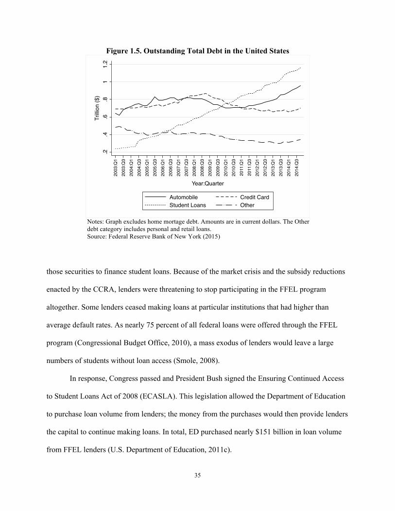
35
Figure 1.5. Outstanding Total Debt in the United States
Notes: Graph excludes home mortage debt. Amounts are in current dollars. The Other debt category includes personal and retail loans. Source: Federal Reserve Bank of New York (2015)
those securities to finance student loans. Because of the market crisis and the subsidy reductions
enacted by the CCRA, lenders were threatening to stop participating in the FFEL program
altogether. Some lenders ceased making loans at particular institutions that had higher than
average default rates. As nearly 75 percent of all federal loans were offered through the FFEL
program (Congressional Budget Office, 2010), a mass exodus of lenders would leave a large
numbers of students without loan access (Smole, 2008).
In response, Congress passed and President Bush signed the Ensuring Continued Access
to Student Loans Act of 2008 (ECASLA). This legislation allowed the Department of Education
to purchase loan volume from lenders; the money from the purchases would then provide lenders
the capital to continue making loans. In total, ED purchased nearly $151 billion in loan volume
from FFEL lenders (U.S. Department of Education, 2011c).
.2.4
.6.8
11.
2Tr
illion
($)
2003
:Q1
2003
:Q3
2004
:Q1
2004
:Q3
2005
:Q1
2005
:Q3
2006
:Q1
2006
:Q3
2007
:Q1
2007
:Q3
2008
:Q1
2008
:Q3
2009
:Q1
2009
:Q3
2010
:Q1
2010
:Q3
2011
:Q1
2011
:Q3
2012
:Q1
2012
:Q3
2013
:Q1
2013
:Q3
2014
:Q1
2014
:Q3
Year:Quarter
Automobile Credit CardStudent Loans Other

36
To ensure that students could borrow enough to finance their education, the ECASLA
also increased Stafford loan limits (see Table 1.1). Effective July 1, 2008, the total annual loan
limit increased $2,000 for both dependents and independents. With this change, the annual
Stafford loans limits, for the first time, are greater than the annual subsidized limits for
dependent students. ECASLA also increased the aggregate loan limit for dependents by $8,000,
from $23,000 to $31,000. For independents, the aggregate limit increased $11,500, from $46,000
to $57,500.
For parents borrowing PLUS loans, the ECASLA provided repayment relief. Prior to the
ECASLA, parental PLUS loans entered repayment within 60 days of disbursement. ECASLA
amended the Higher Education Act to allow parent PLUS loan borrowers to defer repayment
while their child was enrolled in school.
1.4.3.2. 2008 Reauthorization of the Higher Education Act
After the passage of the ECASLA, Congress revisited reauthorization of the HEA. The
last comprehensive reauthorization occurred in 1998. Until 2008, Congress temporarily extended
HEA provisions fourteen times (Smole, Kuenzi, & Skinner, 2008). In light of legislators’
preoccupation with the upcoming Congressional and Presidential elections and the recent
reforms implemented by the CCRA and the ECASLA, this reauthorization would not be
comprehensive. The reauthorization legislation, The Higher Education Opportunity Act of 2008
(HEOA), instead tackled technical amendments that had not been addressed since the 1992 and
1998 Reauthorizations.
Specific to federal student loans, the HEOA increased annual and aggregate Perkins loan
limits and created two new loan forgiveness programs (Smole et al., 2008). The first is designed
to grant borrowers employed full-time in an area of national need receive up to $10,000 in loan

37
forgiveness. However, Congress has yet to fund this program (Hegji, Smole, & Heisler, 2014).
The second forgiveness program provides up to $40,000 in loan forgiveness for civil legal
assistance attorneys. Additionally, the HEOA altered the method used to determine cohort
default rates. Previously, the default rate was based on the share of borrowers who defaulted
within a 2-year repayment period. The HEOA extended the 2-year period to 3 years, as a result,
default rates increased significantly (see Figure 1.3 for a comparison of the 2-year and 3-year
default rates).
For the Pell grant, the HEOA increased the maximum authorized award amounts for the
first time since the 1998 Reauthorization. The authorized maximum was set to gradually increase
to $8,000 in 2014. Because funding has to be appropriated annually, the Pell maximum
consistently fell below these authorized levels by as much as $2,500. One initiative that President
Bush advocated for and included in the HEOA was the ability for students to receive a Pell grant
year round (Delisle & Miller, 2015). Under this plan, a student could receive a Pell grant for the
summer in addition to the regular academic year. Two years later, year-round Pell was
eliminated in order to reduce the overall cost of the Pell grant program.
1.4.3.3. The Move to Full Direct Lending
When President Obama took office in 2009, he argued that federal Stafford loans would
be better served under the Direct Loan program, as opposed to the FFEL program. The market
crisis in 2008 and the threat of lenders’ withdrawing from the FFEL program illustrated the
vulnerability inherent in relying on external lenders to make federal loans. Support for Obama’s
plan grew when the Congressional Budget Office (2010) estimated that replacing the FFEL with
direct lending would save the government $87 billion. In his State of the Union Address,
President Obama urged Congress to pass a bill that “will finally end the unwarranted taxpayer
38
subsidies that go to banks for student loans.” Further, he advocated for student debt relief,
stating, “Let's tell another 1 million students that when they graduate, their student loan
payments will be limited to 10 percent of their income and all of their debt will be forgiven after
20 years.”
On March 30, 2010, President Obama signed the Health Care and Education
Reconciliation Act, which officially ended external lender participation in federal loan programs
and required all future student loans to be processed though the Direct Loan program. The
legislation also created a new loan repayment program, called Pay as You Earn, to be financed
with savings generated by eliminating the FFEL. Pay as You Earn allows borrowers’ monthly
payment to be adjusted for annual income and for debt to be forgiven after 20 years (Dortch,
Smole, & Mahan, 2010). Additionally, the Pell grant also received an increase of $13 billion in
mandatory spending.
1.4.3.4. Interest Rate Changes In 2013, the CCRA provisions that reduced subsidized Stafford loan interest rates to a
fixed 3.4 percent were set to expire and rates were scheduled to revert back to 6.8 percent.
Federal policymakers had different ideas as to how the rates should be determined. President
Obama advocated for tying interest rates to Treasury securities (Field, 2013). Congressional
Republicans also wanted interest rates determined by Treasury securities, but preferred rates one
percentage point higher than the President’s proposal. Congressional Democrats, on the other
hand, proposed freezing rates at 3.4 percent in order to buy time to craft a more permanent
solution. In the end, all parties agreed to a compromise. The Bipartisan Student Loan Certainty
Act of 2013 changed the interest rates on subsidized Stafford loans from fixed to a fixed-variable
hybrid in which the interest rate is adjusted annually for new loans and is fixed for the life of the

39
loan (Gardner, 2013). While the 2013-14 interest rate did increase from 3.4 percent to 3.86
percent, the outcome was more favorable for borrowers than the scheduled jump to 6.8 percent.
1.4.3.5. Institutional Accountability with Student Loan Debt
With student loan debt and default rates rising, the Obama administration began to
propose new mechanisms in late 2010 and early 2011 to hold postsecondary institutions
accountable. The proposed rules attempted to monitor the quality of college programs that
prepare students for gainful employment and oversee former students’ level of loan debt (Smole,
2011). One proposed rule measured students’ ability to repay loan debt. Other measures
specified the allowable debt-to-earnings ratio. Under these proposed “gainful employment” rules,
if a college’s program fails to pass at least one of these measures for three out of four years, the
federal government could sanction the college from participation in federal aid programs. In
general, these proposed rules were directed toward for-profit colleges with academic programs
that do not lead to a postsecondary degree.
After the release of these proposed rules, the U.S. Department of Education received over
90,000 comments (Smole, 2011) and for-profit institutions filed several lawsuits against the
Department. In one ruling, a federal judge recognized the need for government oversight of
students’ debt but declared that proposed threshold measures to determine federal sanctions were
“arbitrary and capricious” ("Association of Private Colleges and Universities v. Arne Duncan,"
2012). In response to the court ruling, the U.S. Department of Education proposed a new set of
gainful employment rules in 2014. Compared to the earlier proposals, the rules on repayment rate
were removed, but measures on earnings-to-debt ratios remained. Within weeks of the release of
the new proposal, for-profit institutions filed a lawsuit, which suggests that efforts to promote

40
institutional accountability by establishing aggressive federal oversight are likely to be ongoing
and a lasting source of friction between the government and for-profit institutions.
From 2008 to 2014, the federal government took a more proactive approach in boosting
federal financial aid programs. Though some provisions, including the year-round Pell Grant and
various loan forgiveness programs, were either never implemented or eventually cut to save
money, other reforms offer significant benefits to students. The elimination of the FFEL and
transition to direct lending generated savings to finance interest rate reductions, Pell grant
increases, and new repayment options and loan forgiveness programs to alleviate the burden of
education debt payments. New institutional accountability mechanisms, though tentative and
highly controversial, are designed to prevent students from taking on student loan debt that they
likely will be unable to repay given their economic prospects after graduating or exiting the
program.
Furthermore, there appears to be a growing acknowledgement within the public discourse
and among policymakers that the historical tendency to equate college access with student loan
access and the policies born out of that mindset have promoted a reliance on loans that is
unsustainable and detrimental to both individual students and the economy as a whole. Though
meaningful action has not yet been taken to reverse the trend, ideas are emerging in new
proposals. President Obama, for example, has advocated for allowing students to attend
community colleges tuition free. This approach, which Congress has yet to consider, has the
potential to significantly reduce the use of student loans. Additionally, President Obama has
proposed a new initiative, the “Student Aid Bill of Rights,” which calls for federal action to
improve student loan servicing and create new programs to help borrowers manage their debt.
41
The details of this initiative have yet to be announced, but the intentions demonstrate that
policymakers are taking steps to make college affordable and student loan debt manageable.
1.5. Conclusion Over the past two decades, college tuition has risen faster than inflation and the
purchasing power of need-based grants has not been able to keep pace. In 2012-13, for example,
the Pell grant covered 30 percent of the cost of attendance at public 4-year institutions and less
than 15 percent at private 4-year institutions (College Board, 2014b). To finance the growing
portion of college costs not covered by need-based grants and to compensate for stagnate middle-
class incomes, students and their families are taking out more loans and borrowing larger
amounts. As a result, student loans account for over 50 percent of all federal aid provided to
students. The annual share of students borrowing has increased from 26 percent in 1995-96 to 42
percent in 2011-12. Currently, over two-thirds of students graduate from college with an average
debt load greater than $28,000 (The Institute for College Access & Success, 2014b). At $1.12
trillion, student loan debt is now the second largest form of debt behind home mortgages.
Hearn’s 1998 paper examined the history of federal loan policies and explained how
policy changes contributed to the growth of federal loans in the financial aid system. This paper
picked up where Hearn left off, documenting how federal loan policies have continued to
promote student loans as a dominant mechanism for paying college costs and describing how
specific policy changes have contributed to escalating debt.
Although the nature and intent of financial aid provisions since the early 1990s varied
widely, their implementation perpetuated the shift away from grant aid and toward loans and
sought to expand college access by allowing more students to borrow larger loans. Rather than
examining why middle-income families were increasingly unable to pay for college and

42
addressing college affordability, for example, Congressional action during the 1990s expanded
loan eligibility for middle-income students. Grant aid was funded at stagnant levels while new
aid programs, such as tax credits, were created, and initiatives that expanded loan access
allocated more resources to loan programs. Other salient policy changes included increases in
annual and aggregate loan limits; today dependent students can graduate with almost $31,000 in
federal student loan debt, and that figure surges to $57,500 for independent students.
Furthermore, the legislative response in more recent years to escalating default rates and
the overall student loan debt has focused on reforming repayment rather than reducing the
reliance on loans. Congress introduced a plethora of new income-contingent repayment plans
and loan forgiveness programs and supported loan consolidation. All of which extended
borrowers’ repayment terms and provided additional relief for borrowers in the short-term.
While these provisions may help students already in repayment, they fail to address the
underlying source of the problem and prevent current and future college students from
graduating with high debt loads and ending up in similar situations to borrowers currently in
repayment.
Recent initiatives proposed by President Obama do reflect the growing realization that
increasing the availability and amount of loans is not a viable mechanism for expanding access
to and affordability of postsecondary education, but no meaningful action has been taken thus
far. Given the ways in which the federal policies highlighted in this paper shaped the existing
financial aid system and the difficulty passing and implementing sweeping reforms encountered
in the past, however, the nature of policymakers’ response to the current crisis will likely have
lasting consequences for future students and their families.
43
Appendix 1
Appendix 1.A. Who can Borrow a Stafford Loans?
Any student, regardless of their financial circumstances, can receive a Stafford subsidized
or unsubsidized loan. In order to receive a loan, students must first complete the Free
Application for Federal Student Aid (FAFSA) - an application containing over 100 questions that
collects information on earned income, assets, family size, and the number of family members
attending college for the year. Once individuals complete and submit the application, the
Department of Education uses the information to calculate the Expected Family Contribution
(EFC), which is “a measure of how much the student and his or her family can be expected to
contribute to the cost of the student’s education for the year” (U.S. Department of Education,
2014a, p. AVG-37).
The type of loan a student receives depends on their financial need. Need is defined as
the difference between the student’s cost of attendance (COA) and expected family contribution
(EFC) (Need = COA - EFC). Cost of attendance is a measure of the amount that students are
charged by the institution. This includes tuition and fees, as well as room and board (if the
student lives on campus) or rent (if the student lives off campus), books, and transportation.
Financial aid administrators develop aid packages consisting of grants and scholarships that are
tailored to reduce students’ need. Subsidized loans are last dollar and fill in the remaining need
after the application of grants and scholarships. Unsubsidized are also last dollar, but are not
given to the student based on remaining need.
44
Even when aid administrators offer loans to students, it does not mean students are
obligated to take the full amount. Students have discretion on the loan amount they wish to
borrow, so long as the amount does not exceed the loan amount offered by the financial aid
administrator. An example can be illustrated with a 1st year student who has a COA of $10,000
and an EFC of $2,000. The student’s financial need is $8,000. Assuming the student received
federal, state, and institutional grants totaling $5,600, the remaining financial need is $2,400.
This remaining amount of need could be covered with a subsidized loan totaling up to $2,400.
Because eligibility for an unsubsidized loan is not determined by financial need, the student has
the option to cover their EFC with this loan. In this case, the student has the opportunity to
borrow up to the total loan amount of $4,400, with no more than $2,400 being subsidized.
Appendix 1.B. Federal Loan Repayment Plans After graduating from college, borrowers are provided with various loan repayment
plans, which are standard, graduate, extended, income-contingent, income-based, Pay-As-You
Earn, and income-sensitive. The standard and graduated plans allow borrowers to repay their
loans in 10 years, but the monthly repayment amount varies. With standard repayment,
borrowers will repay the loan in equal sizes every month. Under a graduate repayment plan,
borrowers will start with lower monthly payments, which will gradually increase until the loan is
paid off. Extended repayment is similar to standard and graduates, but borrowers have 25 years
to fully repay the loan.
The remaining repayment plans offer more flexibility with regards to a borrower’s
income. The income-contingent plan allows monthly payments to be adjusted annually based on
borrowers’ adjusted gross income (AGI), family size, and the total amount of the loan. The
income-based provides for monthly payments that are determined annually by taking 15 percent

45
of the difference between students’ AGI and the 150 percent of the poverty thresholds for the
borrowers’ family size. Pay-As-You Earn is very similar to the income-based repayment, but the
monthly payments are determined from 10 percent of the difference between AGI and poverty
thresholds. All of the aforementioned plans with income adjusted repayments offer loan
forgiveness at the end of the repayment period, which can be equal to or greater than 20 years.
For example, if a student using the income-based repayment plan and was not apply to fully
repay the loan after 25 years, the outstanding loan balance will be forgiven. The last repayment
plan, income-sensitive, is for FFEL loans only and does not offer loan forgiveness. The monthly
payment for income-sensitive is annually adjusted and based on the borrower’s income.
As Table 1.5 displays, roughly 40 percent of outstanding Safford loans are being repaid
under the standard plan. The second most popular repayment plan is income-based at 22 percent.
In general, Table 1.5 illustrates that a majority of outstanding loans fall into plans that have set
monthly payment, as opposed to a monthly payment that is income adjusted.
Table 1.5. Repayment Plans for Outstanding Stafford Loans
Repayment Plan Share of Federal Loan Volume
in Repayment Standard: 10 years or less 39.8% Extended: More than 10 years 12.3% Graduated: 10 years or less 10.6% Graduated-Extended: More than 10 years 2.0% Income-Contingent 3.5% Income-Sensitive 0.0% Income-Based 22.0% Pay As You Earn 2.8% Alternative 1.1% Other 5.9% Note: Total outstanding federal loan volume was $597.2 billion as of December 31, 2014. Loan volume includes loans in repayment, deferment, and forbearance and excludes borrowers in default, in school, and grace. Source: (U.S. Department of Education, 2014c)

46
Borrowers also have the opportunity to have their debt relieved through a variety of
federal and state aid programs that forgive loans in exchange for work in occupations that are
considered to be in high demand. In an examination of state loan forgiveness programs,
Kirshstein, Berger, Benatar, and Rhodes (2004) and Wiederspan (2011) both found that a
majority of these programs are targeted to borrowers going into teaching, nursing, and medical
occupations. At the federal level, there are several loan forgiveness programs and a conditional
grant/loan for teachers and individuals working in the public sector. A discussion on the
difference between loan forgiveness and conditional grant/loan programs is in Appendix 1.D.
Appendix 1.C. Federal Support for Financial Aid
Table 1.6. Description of Federal Aid Programs Pell Grants Formerly known as the Beginning Education Opportunity Grant (BEOG) and is
the largest need-based aid program in the United States. Currently, students can receive a grant amount up to $5,550. The amount of the award depends upon EFC and enrollment intensity.
Supplemental Education Opportunity Grant (SEOG)
SEOG is a campus-based aid program. Colleges match federal funds. Not all college participates. Provided to students with extremely high financial need, with amounts up to $4,000.
Leveraging Educational Assistance Partnership (LEAP)
Previously known as the State Student Incentive Grant (SSIG). Program ended in 2011-12. LEAP provided grants to states to create need-based grants. States determined eligibility and award amounts.
Academic Competitiveness Grants (ACG)
Started in 2006-07 and ended in 2011-12. Awarded to Pell Grant eligible students in their 1st and 2nd year of college enrollment and completed a rigorous high school program. Student could have received a grant amount up to $1,300.
SMART Started in 2006-07 and ended in 2011-12. Awarded to Pell Grant eligible students in their 3rd and 4th year of college enrollment and majoring in technical fields, foreign languages, or in a qualified liberal arts program. Students could have received a grant amount up to $4,000.
Work-Study Is a campus-based aid program and provides students with part-time work on-campus. Colleges determine the hourly wage, and the amount earned cannot exceed the amount awarded.
Veterans and Military Benefits Benefits are education related payments to veterans, military personnel, or students whose parent/s died during military service. These benefits are non-need-based.
Hope Scholarship Provided a maximum credit of $1,800 for tuition and fee expenses. Credit was only available for students in their first two years of enrollment. The AOTC replaced the Hope Scholarship in 2009.
Lifetime Learning Credit (LLC) Allows for a tax credit up to $2,000 for qualified education expenses. American Opportunity Tax Credit (AOTC)
AOTC replace the Hope Scholarship in 2009 and allows for a credit up to $2,500 for expenses related to tuition and fees and course materials. The amount of the credit is 100 percent for the first $2,000 of qualified education expenses and 25 percent for the next $2,000.

47
Appendix 1.D. Description of Loan Forgiveness and Conditional Grant/Loan Programs
In 1998, Congress created a loan forgiveness program that allowed teachers to have
$5,000 of their Stafford loans forgiven after five years of teaching in a low-income school. In
2004, Congress passed legislation that supplemented the 1998 teacher loan forgiveness program
by raising the forgiveness amount to $17,500 for teachers in mathematics, science, or special
education. Congress approved of another loan forgiveness program in 2007 that relieved a
student’s loan debt in exchange for their employment in a public sector job, which includes
military service, nursing, first responders, and general employment for an organization that is
considered to be a 501(c)(3) (non-profit). Congress created a conditional grant/loan in 2007
called the Teacher Education Assistance for College and Higher Education (TEACH), which
provides up to $4,000 annually in grants to students who intend to teach full-time in high-need
subject areas at low-income schools. If the student does not fulfill the teaching obligations within
eight years after graduating from college, the grant converts to a loan.
Loan forgiveness and conditional grant/loan programs have one or more of the following
goals: to provide financial assistance for students to pay for college by reducing individuals’
dependency on student loans; to persuade individuals to choose a specific college major or career
occupation; to attract individuals to work in a job or underserved region for specific period of
time; or to encourage individuals to work and remain in either a occupation of high need and/or a
specific region (McCallion, 2005). Understanding the difference between the two programs can
be confusing, as there is not a universally accepted definition of these programs by researchers
and policymakers. For example, “conditional grants” may sometimes be referred to as “loan
forgiveness programs” and “loan forgiveness programs” may sometimes be labeled as “loan
repayment programs” (McCallion, 2005; see Spero, 1986, & Maplethorpe, 2001, as an example).
48
Despite the mismatch in labels, researchers can distinguish the two programs by how they
operate and are administered. For a conditional grant/loan, the recipient receives the award while
in school and has to fulfill certain service or work requirements after graduating (National
Association of State Student Grant and Aid Programs, 2010). If the recipient fails to fulfill the
service obligations, the award becomes a loan that the recipient pays back. With loan
forgiveness, the recipient is able to have the loan repaid or forgiven, in whole or in part, after
fulfilling certain service or work obligations (NASSGAP, 2010). Typically, if the recipient fails
the service obligations after a pre-determined period of time, the recipient becomes ineligible to
have his/her loan forgiven. In other words, the difference between the two programs is that
conditional grants or loans operate while the student is in school while loan forgiveness works to
help the student after he or she graduates.
To illustrate the operation of conditional grants and loan forgiveness, Figure 1.6
compares the programs in terms of a student paying for college with a student loan. In Figure
1.6, there are three students paying $5,000 in tuition at a university, with student 1 receiving a
conditional grant worth $5,000 and both students 2 and student 3 financing their degree with a
$5,000 loan. Student 2 is majoring in a certain field knowing that he/she will be eligible to have
the loan forgiven if working in a public sector occupation. At the end of college, both students 1
and 2 must make a decision of whether to enter the public sector. If the student(s) decide to
fulfill their service requirements, the student(s) would be relieved of having to incur debt.
Fundamentally, both conditional grants and loan forgiveness programs have the same payoff for
service and have similar results when one does not fulfill the service requirement. If students 1
and 2 decide not to go into the public sector, both will incur a loan debt and will make loan
repayments similar to those of student 3.
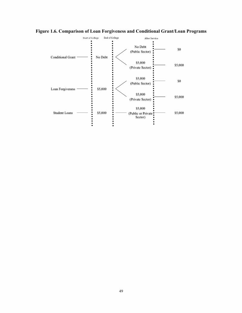
49
Figure 1.6. Comparison of Loan Forgiveness and Conditional Grant/Loan Programs
50
Chapter 2. Denying Loan Access: The Student-Level Consequences When Community Colleges Opt Out of the Stafford Loan
Program
2.1. Introduction
Over the past two decades, rising college tuition rates and a decline in the purchasing
power of need-based grants have lead student loans to become a key component of the financial
aid system in the United States. According to the College Board (2013), over 8 million
undergraduates borrow federal loans each year, and for the 2011-12 academic year, the federal
government provided over 80 billion in Stafford loans. In comparison, roughly 34 billion was
spent on the Pell grant, the nation’s largest need-based grant program. For 2013, over two-thirds
of students graduating from college had an average debt load of $28,400, which is up 2% from
the year before (The Institute for College Access & Success, 2014b)
Students using loans to pay for college and the resulting debt have been central to the
broader national dialogue concerning rising debt levels. The nation’s student loan debt grew
$124 billion this past year and has become the second largest form of debt at $1.12 trillion
(Federal Reserve Bank of New York, 2014). This trend has led to growing concern that the U.S.
is facing a student loan debt crisis (Kamenetz, 2006; Salas Gage & Lorin, 2014), as increasing
debt levels, fewer employment opportunities and low salaries leave some borrowers struggling to
repay (Consumer Financial Protection Bureau, 2013). Nationally, student loan default rates have
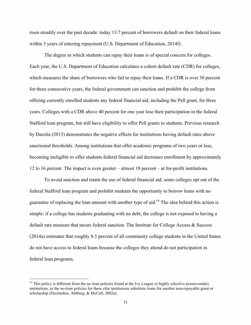
51
risen steadily over the past decade: today 13.7 percent of borrowers default on their federal loans
within 3 years of entering repayment (U.S. Department of Education, 2014f).
The degree to which students can repay their loans is of special concern for colleges.
Each year, the U.S. Department of Education calculates a cohort default rate (CDR) for colleges,
which measures the share of borrowers who fail to repay their loans. If a CDR is over 30 percent
for three consecutive years, the federal government can sanction and prohibit the college from
offering currently enrolled students any federal financial aid, including the Pell grant, for three
years. Colleges with a CDR above 40 percent for one year lose their participation in the federal
Stafford loan program, but still have eligibility to offer Pell grants to students. Previous research
by Darolia (2013) demonstrates the negative effects for institutions having default rates above
sanctioned thresholds. Among institutions that offer academic programs of two years or less,
becoming ineligible to offer students federal financial aid decreases enrollment by approximately
12 to 16 percent. The impact is even greater – almost 18 percent – at for-profit institutions.
To avoid sanction and retain the use of federal financial aid, some colleges opt out of the
federal Stafford loan program and prohibit students the opportunity to borrow loans with no
guarantee of replacing the loan amount with another type of aid.14 The idea behind this action is
simple: if a college has students graduating with no debt, the college is not exposed to having a
default rate measure that incurs federal sanction. The Institute for College Access & Success
(2014a) estimates that roughly 8.5 percent of all community college students in the United States
do not have access to federal loans because the colleges they attend do not participation in
federal loan programs.
14 This policy is different from the no-loan policies found at the Ivy League or highly selective postsecondary institutions, as the no-loan policies for these elite institutions substitute loans for another non-repayable grant or scholarship (DesJardins, Ahlburg, & McCall, 2002a).
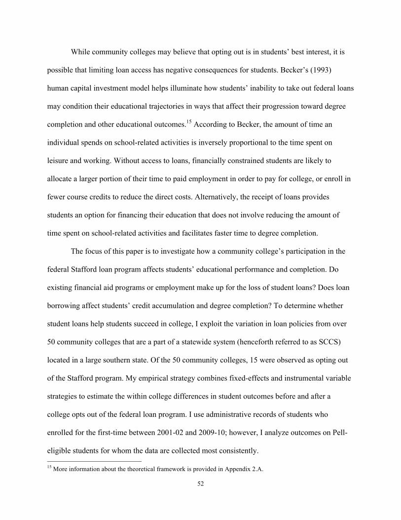
52
While community colleges may believe that opting out is in students’ best interest, it is
possible that limiting loan access has negative consequences for students. Becker’s (1993)
human capital investment model helps illuminate how students’ inability to take out federal loans
may condition their educational trajectories in ways that affect their progression toward degree
completion and other educational outcomes.15 According to Becker, the amount of time an
individual spends on school-related activities is inversely proportional to the time spent on
leisure and working. Without access to loans, financially constrained students are likely to
allocate a larger portion of their time to paid employment in order to pay for college, or enroll in
fewer course credits to reduce the direct costs. Alternatively, the receipt of loans provides
students an option for financing their education that does not involve reducing the amount of
time spent on school-related activities and facilitates faster time to degree completion.
The focus of this paper is to investigate how a community college’s participation in the
federal Stafford loan program affects students’ educational performance and completion. Do
existing financial aid programs or employment make up for the loss of student loans? Does loan
borrowing affect students’ credit accumulation and degree completion? To determine whether
student loans help students succeed in college, I exploit the variation in loan policies from over
50 community colleges that are a part of a statewide system (henceforth referred to as SCCS)
located in a large southern state. Of the 50 community colleges, 15 were observed as opting out
of the Stafford program. My empirical strategy combines fixed-effects and instrumental variable
strategies to estimate the within college differences in student outcomes before and after a
college opts out of the federal loan program. I use administrative records of students who
enrolled for the first-time between 2001-02 and 2009-10; however, I analyze outcomes on Pell-
eligible students for whom the data are collected most consistently. 15 More information about the theoretical framework is provided in Appendix 2.A.
53
I find that Pell-eligible students enrolling when the community college offered federal
loans are 7.6 percentage points more likely to borrow than students who enrolled after the
community college opted out of the federal loan program. The overall amount borrowed also
increases $368. I also find that after the switch in loan policy, institutions did not replace the loss
in loan amounts with another financial aid program. I find no evidence that loan borrowing
statistically improves degree completion and transfer to a 4-year institution, but do find that Pell-
eligible students borrowing a loan attempted 19 additional credits and were more likely to
attempt and complete math and science courses than non-borrowers.
In Section 2.2, I describe previous research on student loans in order to illustrate the lack
of research examining the relationship between loan borrowing and students’ educational
outcomes. Section 2.3 highlights students’ loan use within SCCS and explanations for why
SCCS colleges opt out of the federal loan program. Sections 2.4 and 2.5 describe the data and
sample used for analysis. Section 2.6 describes my empirical strategy. Results are in Section 2.7
and concluding thoughts are in Section 2.8.
2.2. Research on Students Loans
Researchers know little about whether loans help students succeed in college. In theory,
the availability of loans removes credit constraints and affords educational opportunities to many
students who may not otherwise have been able to attend college. However, the findings on
student loans have been inconsistent. Some studies have found that loans exert a positive
influence on college outcomes (Chen & DesJardins, 2008; Cofer & Somers, 2000), while others
have found insignificant or negative effects (Braunstein, McGrath, & Pescatrice, 2000-2001;
DesJardins, Ahlburg, & McCall, 2002b; Dowd & Coury, 2006).

54
Estimating the effects of loans on college outcomes can be difficult because students’
loan receipt is not randomly assigned. In the United States, the federal loan program is designed
in such a way that students self-select their loan amount. Simply comparing outcomes between
student loan borrowers and non-borrowers is likely to produce biased estimates because there are
possible unobserved differences between the two groups that could be associated with the
decision on whether or not to borrow. In absence of a randomized experiment, the challenge is to
counteract this self-selection bias. More recently, researchers have begun to employ quasi-
experimental approaches by exploiting an exogenous assignment that determines whether a
student is eligible for a loan. This approach allows for the development of a counterfactual of
what students would do in absence of receiving a loan.
Two studies examining student loan programs outside of the United States employ a
quasi-experimental research method and find positive effects with loan eligibility. Both of these
studies use a regression discontinuity design around a minimum score that determines whether or
not a student can be offered a loan. Gurgand, Lorenceau, and Melonio (2011) examined a private
loan program in South Africa, and students whose parents’ credit score was just above the
eligibility threshold were 20 percentage points more likely to enroll in college. Solis (2012)
examined students’ college admission test scores and, like Gurgand, et. al. (2011), found a 20
percentage point increase in the probability of enrollment with eligibility for loan programs in
Chile. Additionally, Solis found that access to loans lead to a lower dropout rate, as loan eligible
students were more likely to enroll in the second and third years of college.
Of the studies evaluating student loans in the United States, most of the research
examines student loans in relationship to college enrollment or post-college employment
decisions. Dynarski (2003) uses a difference-in-difference strategy to examine the change in

55
federal loan availability with the removal of home equity in the financial aid formula. She found
that federal loan eligibility had a weak effect on college enrollment. Rothstein and Rouse (2010)
evaluated a no-loan policy at a highly selective university where the loan component of students’
financial aid awards was replaced with grants. Their findings suggested that debt increased the
probability of students choosing a high-salary job rather than a job that has low pay or in the
public sector.
There is little research that examines the effect of U.S. loan programs on students’
educational outcomes. In the paper most related to the present analysis, Dunlop (2012) exploits
the variation in community colleges’ participation in the federal Stafford loan program. Using
the Beginning Postsecondary Student Study of 2004, Dunlop uses a community college’s federal
loan participation as an instrument to estimate the effect of the loan amount borrowed on credits
completed, degree attainment, and transfer to a 4-year college. Dunlop mostly interprets findings
from the reduced form estimations, but her results suggest that limiting loan access indeed
decreases loan borrowing and hinders the transfer to a four-year college. Results on other
outcomes, such as credits completed, were statistically insignificant.
Because Dunlop uses cross-sectional variation in community colleges’ loan participation,
the composition of students across colleges could be different. Community colleges operate to
serve the surrounding community, and the composition of the student body could reflect the
community’s socioeconomic characteristics, some of which could be associated with students’
decisions on whether or not to borrow a loan. In addition, colleges are likely to develop academic
and financial aid programs that are tailored to meet the needs of the surrounding area. Dunlop’s
analysis does not fully account for these institutional differences and whether institutions help
students’ make-up for the loss of loan access. To do so would require longitudinal observation
56
within an institution to see how students respond before and after the change in loan policy,
which is the contribution of my paper.
2.3. Loan Policies Within the Statewide Community College System (SCCS)
To analyze how participation in the federal loan program affects students’ education
outcomes, I examine the loan policies from the 50 public community colleges within the SCCS.
In comparison to other community colleges nationwide, SCCS contains a significantly high
number of community colleges that have opted out of the federal Stafford loan program. For
example, during the 2001-02 academic year, over 70 percent of all public 2-year institutions in
the United States participated in the Stafford loan program. In comparison, only 60 percent of
SCCS institutions offered federal loans. By 2009-10, the share of public 2-year participating was
still over 70 percent nationwide, whereas participation among SCCS institutions dropped to
almost 35 percent.
Between 2001-02 and 2009-10, 15 community colleges in the SCCS altered their federal
loan policy. Using data from the U.S. Department of Education’s (2014g) Title IV Program
Volume Reports, Figure 2.1 displays the number of Stafford loans each of the 15 institutions
disbursed to students. At some point, these 15 community colleges opted to not participate in the
federal loan program. The horizontal line indicates when the switch to not offering loans
occurred. Institution 3 is the only the institution altering their loan policy twice: opting out in
2002-03, and then reinstating students’ borrowing privileges in the 2007-08 academic year.
Despite the decrease in the number of SCCS institutions offering federal Stafford loans,
the proportion of its students borrowing has substantially increased. Figure 2.2 displays the
growth in borrowing by incoming cohort for all SCCS institutions over a 9-year period;
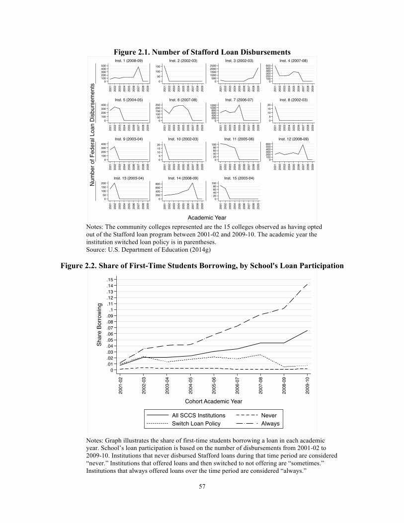
57
Figure 2.1. Number of Stafford Loan Disbursements
Notes: The community colleges represented are the 15 colleges observed as having opted out of the Stafford loan program between 2001-02 and 2009-10. The academic year the institution switched loan policy is in parentheses. Source: U.S. Department of Education (2014g)
Figure 2.2. Share of First-Time Students Borrowing, by School's Loan Participation
Notes: Graph illustrates the share of first-time students borrowing a loan in each academic year. School’s loan participation is based on the number of disbursements from 2001-02 to 2009-10. Institutions that never disbursed Stafford loans during that time period are considered “never.” Institutions that offered loans and then switched to not offering are “sometimes.” Institutions that always offered loans over the time period are considered “always.”
0100200300400500
0
50
100
150
0500
1000150020002500
0100200300400500600
0100200300400
050
100150200250
0200400600800
10001200
05
101520
0100200300400
05
101520
020406080
100
0100200300400500600
050
100150200
0200400600800
020406080
100
2001
2002
2003
2004
2005
2006
2007
2008
2009
2001
2002
2003
2004
2005
2006
2007
2008
2009
2001
2002
2003
2004
2005
2006
2007
2008
2009
2001
2002
2003
2004
2005
2006
2007
2008
2009
2001
2002
2003
2004
2005
2006
2007
2008
2009
2001
2002
2003
2004
2005
2006
2007
2008
2009
2001
2002
2003
2004
2005
2006
2007
2008
2009
2001
2002
2003
2004
2005
2006
2007
2008
2009
2001
2002
2003
2004
2005
2006
2007
2008
2009
2001
2002
2003
2004
2005
2006
2007
2008
2009
2001
2002
2003
2004
2005
2006
2007
2008
2009
2001
2002
2003
2004
2005
2006
2007
2008
2009
2001
2002
2003
2004
2005
2006
2007
2008
2009
2001
2002
2003
2004
2005
2006
2007
2008
2009
2001
2002
2003
2004
2005
2006
2007
2008
2009
Inst. 1 (2008-09) Inst. 2 (2002-03) Inst. 3 (2002-03) Inst. 4 (2007-08)
Inst. 5 (2004-05) Inst. 6 (2007-08) Inst. 7 (2006-07) Inst. 8 (2002-03)
Inst. 9 (2003-04) Inst. 10 (2002-03) Inst. 11 (2005-06) Inst. 12 (2008-09)
Inst. 13 (2003-04) Inst. 14 (2008-09) Inst. 15 (2003-04)
Num
ber o
f Fed
eral
Loa
n D
isbu
rsem
ents
Academic Year
0.01.02.03.04.05.06.07.08.09
.1.11.12.13.14.15
Shar
e Bo
rrow
ing
2001
-02
2002
-03
2003
-04
2004
-05
2005
-06
2006
-07
2007
-08
2008
-09
2009
-10
Cohort Academic Year
All SCCS Institutions NeverSwitch Loan Policy Always
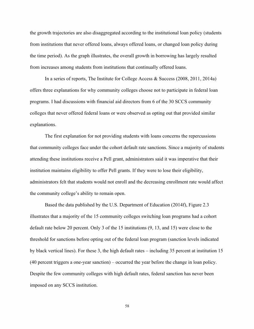
58
the growth trajectories are also disaggregated according to the institutional loan policy (students
from institutions that never offered loans, always offered loans, or changed loan policy during
the time period). As the graph illustrates, the overall growth in borrowing has largely resulted
from increases among students from institutions that continually offered loans.
In a series of reports, The Institute for College Access & Success (2008, 2011, 2014a)
offers three explanations for why community colleges choose not to participate in federal loan
programs. I had discussions with financial aid directors from 6 of the 30 SCCS community
colleges that never offered federal loans or were observed as opting out that provided similar
explanations.
The first explanation for not providing students with loans concerns the repercussions
that community colleges face under the cohort default rate sanctions. Since a majority of students
attending these institutions receive a Pell grant, administrators said it was imperative that their
institution maintains eligibility to offer Pell grants. If they were to lose their eligibility,
administrators felt that students would not enroll and the decreasing enrollment rate would affect
the community college’s ability to remain open.
Based the data published by the U.S. Department of Education (2014f), Figure 2.3
illustrates that a majority of the 15 community colleges switching loan programs had a cohort
default rate below 20 percent. Only 3 of the 15 institutions (9, 13, and 15) were close to the
threshold for sanctions before opting out of the federal loan program (sanction levels indicated
by black vertical lines). For these 3, the high default rates – including 35 percent at institution 15
(40 percent triggers a one-year sanction) – occurred the year before the change in loan policy.
Despite the few community colleges with high default rates, federal sanction has never been
imposed on any SCCS institution.
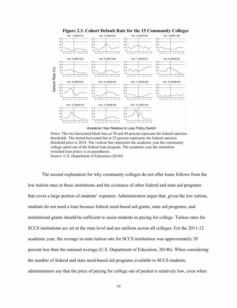
59
Figure 2.3. Cohort Default Rate for the 15 Community Colleges
Notes: The two horizontal black bars at 30 and 40 percent represent the federal sanction thresholds. The dotted horizontal bar at 25 percent represents the federal sanction threshold prior to 2014. The vertical line represents the academic year the community college opted out of the federal loan program. The academic year the institution switched loan policy is in parentheses. Source: U.S. Department of Education (2014f)
The second explanation for why community colleges do not offer loans follows from the
low tuition rates at these institutions and the existence of other federal and state aid programs
that cover a large portion of students’ expenses. Administrators argue that, given the low tuition,
students do not need a loan because federal need-based aid grants, state aid programs, and
institutional grants should be sufficient to assist students in paying for college. Tuition rates for
SCCS institutions are set at the state level and are uniform across all colleges. For the 2011-12
academic year, the average in-state tuition rate for SCCS institutions was approximately 20
percent less than the national average (U.S. Department of Education, 2014b). When considering
the number of federal and state need-based aid programs available to SCCS students,
administrators say that the price of paying for college out of pocket is relatively low, even when
010203040
010203040
010203040
010203040
010203040
010203040
010203040
010203040
010203040
010203040
010203040
010203040
010203040
010203040
010203040
-4 -3 -2 -1 0 1 2 3 4 5 -4 -3 -2 -1 0 1 2 3 4 5 -4 -3 -2 -1 0 1 2 3 4 5 -4 -3 -2 -1 0 1 2 3 4 5
-4 -3 -2 -1 0 1 2 3 4 5 -4 -3 -2 -1 0 1 2 3 4 5 -4 -3 -2 -1 0 1 2 3 4 5 -4 -3 -2 -1 0 1 2 3 4 5
-4 -3 -2 -1 0 1 2 3 4 5 -4 -3 -2 -1 0 1 2 3 4 5 -4 -3 -2 -1 0 1 2 3 4 5 -4 -3 -2 -1 0 1 2 3 4 5
-4 -3 -2 -1 0 1 2 3 4 5 -4 -3 -2 -1 0 1 2 3 4 5 -4 -3 -2 -1 0 1 2 3 4 5
Inst. 1 (2009-10) Inst. 2 (2002-03) Inst. 3 (2002-03) Inst. 4 (2007-08)
Inst. 5 (2004-05) Inst. 6 (2007-08) Inst. 7 (2006-07) Inst. 8 (2002-03)
Inst. 9 (2003-04) Inst. 10 (2002-03) Inst. 11 (2005-06) Inst. 12 (2008-09)
Inst. 13 (2003-04) Inst. 14 (2008-09) Inst. 15 (2003-04)
Def
ault
Rat
e (%
)
Academic Year Relative to Loan Policy Switch
60
considering the cost of attendance.16 If there is any remaining need after the application of
federal and state aid to students’ aid packages, administrators stated that institutional aid or aid
from privately funded sources should be able to cover the remaining balance.
Finally, administrators at some community colleges believe that providing students with
the option of borrowing opens students to the possibility of over-borrowing and taking on debt
that is beyond their means. Heavily indebted students need high-paying jobs in order to make
their loan payments, and defaulting can have serious consequences for students. The geographic
area in which the community college is located plays an important factor in institutions’
decisions to offer loans: several administrators mentioned that the surrounding county has a very
high unemployment rate and few future employment opportunities. Given students’ limited post-
graduation job prospects, administrators believe that providing students with an easily obtainable
loan is a recipe for enduring financial consequences for students and a high default rate for the
institution. Yet, county unemployment data does not suggest there was a significant jump in
unemployment prior to the change in loan policy across the 15 institutions.17 If there was an
uptick in unemployment, it occurs after the change in policy and is reflective of the Great
Recession that occurred in 2008. Additionally, the county unemployment rate for the 15
institutions is fairly close to the state rate between 2000 and 2010.
According to the aid administrators with whom I spoke, the schools do not offset the loss
of the loan with a grant that matches dollar for dollar what the loan would provide. Instead, they
rely on existing federal and state aid programs. When asked what portion of financial aid 16 During the 2010-11 academic year, for example, the average cost for a traditionally aged (less than 24) full-time student living off-campus with a family was almost $8,000.16 For these students, a majority of their financial need is met by the Pell grant, as the maximum award for that year was $5,500 and covered 68 percent of the cost. However, the cost of attendance for a full-time student who does not live with his or her parents can be upwards of $15,000. While federal grants can cover a portion of their financial need, these students can rely on the various state aid programs specific to community colleges and public institutions in the state. The award amounts from these programs range from $1,500 up to $4,000. 17 Figure 2.5 in Appendix 2.B displays the county unemployment rates for the 15 community colleges.

61
applicants is eligible for a Pell grant, all administrators interviewed estimated figures between 85
to 90 percent.18 Most of these Pell-eligible students have their direct costs covered with existing
aid programs. But what about the 10 to 15 percent who are ineligible for a Pell grant? They lose
loan eligibility when their institution opts out, and a small fraction of these students are eligible
to receive a grant through the various state aid programs. Administrators also mentioned they
have institutional grants available for these students, but noted that not all students will be
eligible, especially ones with higher expected family contributions.
At some SCCS institutions, the decision to opt out of the federal Stafford loan program
does not necessarily apply to private loans. Compared to federal loans, a private loan does not
provide flexible repayment options and traditionally carries higher interest rates. Because the
federal government does not back this type of loan, private loans are not considered in an
institution’s cohort default rate. Consequently, some colleges direct students to private lenders to
avoid federal sanction. On the website for one SCCS institution, for example, the financial aid
office explicitly states that the college does not participate in the federal loan program, but if
students would like to take out a loan, the financial aid webpage suggests that students borrow
through a private lender. Currently, however, the use of private loans among SCCS students
appears to be relatively small. According to SCCS administrative data, less than 1 percent of
students borrow a non-federal loan.19 This should be regarded as a lower bound estimate,
however, as students may take out a private loan and not report it to the college’s financial aid
office.
18 Using SCCS administrative files, 37 percent of all SCCS students receive a Pell grant. Among aid recipients, 75 percent receive a Pell grant. 19 Only students who report to the college that they borrowed a private loan will be reflected in the administrative data.
62
2.4. Data Description
For my analysis, I use student-level administrative records from the over 50 public,
degree-granting community colleges that are part of the SCCS. The records reflect reporting for
each semester students are enrolled for-credit between the 2001-02 and 2009-10 academic years.
This dataset includes detailed information on student demographics, receipt of financial aid,
courses taken, credits attempted and completed, grades earned, and degrees received. In total,
there are over 600,000 students represented in the administrative dataset.
These student records were also matched to the student-level database maintained by the
National Student Clearinghouse (NSC) and the state’s Unemployment Insurance (UI) records.20
The NSC tracked students’ enrollment at postsecondary institutions from 1997 to 2012, allowing
me to examine the students’ post-secondary enrollment prior and subsequent to enrollment in the
SCCS. The NSC data contains information on degrees received, fields of study, and the duration
of enrollment at a particular institution.
The UI records provide an opportunity to examine students’ earnings and employment
both while enrolled in and after their exit from a postsecondary institution. There is one
limitation to using the UI records as a measure of employment, however, because earnings are
reported quarterly and the records do not include information on the number of hours the
individual worked. Data on hours worked would provide more accurate estimates of the time
directed to employment rather than school-related activities. Instead, I align the quarterly
earnings to the term schedules at the community colleges. This approach allows me to calculate
students’ total income during a semester in which they are enrolled. I use 4th quarter wages as a
20 It is worth noting that the UI records reflect in-state employment and excludes earnings from out-of-state or self-employment. For concerns of students working out-of-state, a sensitivity check was conducted by estimating outcomes excluding students attending college near the state boarder. The results did not change from my main findings.
63
measure of employment participation and wages for the fall semester, 1st quarter for the winter
semester, and the 2nd quarter for the spring/summer semester.
I identify whether or not a community college opts out of the federal Stafford loan
program in a given year using financial aid program data from the U.S. Department of Education
(2014g). This data provides information on the total volume of federal loans disbursed by higher
education institutions. I consider a community college as not participating in the federal loan
program when the number of loan disbursements for subsidized and unsubsidized Stafford loans
is 0.21
To account for time varying college characteristics, I use data from the Bureau of Labor
Statistics (2014) and the Delta Cost Project (2014). Data from the BLS provides measures on
county unemployment rates. The Delta database is derived from data reported in the Integrated
Postsecondary Education Data System and includes measures on institutional expenditures.22 For
this study, I use expenditures on student services, academic support, and scholarships and
fellowships.
2.5. Sample Description There are 603,522 first-time students from all 50 community colleges represented in the
SCCS administrative files. One limitation to the SCCS financial aid data is that it consists of only
295,494 students who received financial aid during their enrollment in a SCCS community
college. This means that financial aid information, such as Expected Family Contribution (EFC)
and aid amounts, is missing for any student who did not receive any financial aid. The lack of
information on these non-financial aid recipients makes it problematic to compare students
21 For a small number of community colleges, the total number of loan disbursements from 2001-02 to 2009-10 was less than 10 at each community college and the disbursements would happen in one year. It is unclear why these institutions would have an outlying year by disbursing a small number of loans. For those colleges that have a single, small disbursement year, I recoded the disbursement to 0. 22 Delta Cost data provides consistent measures for variables that may have changed overtime in the IPEDS data.

64
within and across institutions, because a change in loan policy potentially alters the composition
of students represented in the financial aid dataset. For example, a student with a financial aid
package consisting of only loans from the period when the institution participated in the federal
loan programs appears in the data. But a similar student attending the same institution after the
college stopped offering federal loans would not appear in the financial aid dataset.
To account for this data limitation, I use a sample of 206,255 Pell-eligible students with
the assumption that if a student applied for financial aid and was Pell-eligible, the student would
take the Pell Grant they were offered and would be represented in the financial aid dataset
regardless of the institution’s loan policy. From a policy point of view, focusing on Pell-eligible
students is important because this segment of the student population is most sensitive to changes
in college price and financial aid (Heller, 1997). Any changes in aid amounts or limiting access
to aid programs that are intended to improve persistence and completion rates should be
examined to determine whether such action is beneficial for this subset of students.
It is important to discuss how limiting the sample to Pell grant students relates to the
interpretation of the results. This paper does not fully address the impacts of student loans
replacing other forms of financial aid (i.e. only borrowing a loan with no other aid versus no
financial aid at all). Because the sample includes Pell grant recipients, results should be
interpreted as the effect of student loans supplementing grant aid.
To better understand how Pell-eligible students in SCCS compare to all SCCS students,
Table 2.1 presents the summary statistics for all 603,522 students in SCCS (column 1) and
206,255 Pell-eligible students (Column 2). Only column 1 includes both aid and non-aid
recipients. The first row for each variable in Table 2.1 displays the average values and the second
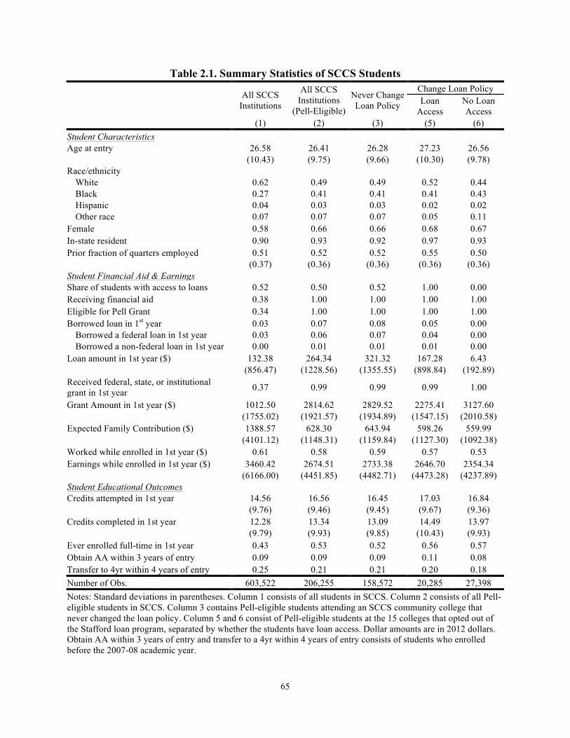
65
Table 2.1. Summary Statistics of SCCS Students
All SCCS Institutions
All SCCS Institutions
(Pell-Eligible)
Never Change Loan Policy
Change Loan Policy Loan
Access No Loan Access
(1) (2) (3) (5) (6) Student Characteristics Age at entry 26.58 26.41 26.28 27.23 26.56
(10.43) (9.75) (9.66) (10.30) (9.78) Race/ethnicity
White 0.62 0.49 0.49 0.52 0.44 Black 0.27 0.41 0.41 0.41 0.43 Hispanic 0.04 0.03 0.03 0.02 0.02 Other race 0.07 0.07 0.07 0.05 0.11
Female 0.58 0.66 0.66 0.68 0.67 In-state resident 0.90 0.93 0.92 0.97 0.93 Prior fraction of quarters employed 0.51 0.52 0.52 0.55 0.50
(0.37) (0.36) (0.36) (0.36) (0.36) Student Financial Aid & Earnings Share of students with access to loans 0.52 0.50 0.52 1.00 0.00 Receiving financial aid 0.38 1.00 1.00 1.00 1.00 Eligible for Pell Grant 0.34 1.00 1.00 1.00 1.00 Borrowed loan in 1st year 0.03 0.07 0.08 0.05 0.00
Borrowed a federal loan in 1st year 0.03 0.06 0.07 0.04 0.00 Borrowed a non-federal loan in 1st year 0.00 0.01 0.01 0.01 0.00
Loan amount in 1st year ($) 132.38 264.34 321.32 167.28 6.43
(856.47) (1228.56) (1355.55) (898.84) (192.89) Received federal, state, or institutional
grant in 1st year 0.37 0.99 0.99 0.99 1.00
Grant Amount in 1st year ($) 1012.50 2814.62 2829.52 2275.41 3127.60
(1755.02) (1921.57) (1934.89) (1547.15) (2010.58) Expected Family Contribution ($) 1388.57 628.30 643.94 598.26 559.99
(4101.12) (1148.31) (1159.84) (1127.30) (1092.38) Worked while enrolled in 1st year ($) 0.61 0.58 0.59 0.57 0.53
Earnings while enrolled in 1st year ($) 3460.42 2674.51 2733.38 2646.70 2354.34
(6166.00) (4451.85) (4482.71) (4473.28) (4237.89) Student Educational Outcomes Credits attempted in 1st year 14.56 16.56 16.45 17.03 16.84
(9.76) (9.46) (9.45) (9.67) (9.36) Credits completed in 1st year 12.28 13.34 13.09 14.49 13.97
(9.79) (9.93) (9.85) (10.43) (9.93) Ever enrolled full-time in 1st year 0.43 0.53 0.52 0.56 0.57 Obtain AA within 3 years of entry 0.09 0.09 0.09 0.11 0.08 Transfer to 4yr within 4 years of entry 0.25 0.21 0.21 0.20 0.18 Number of Obs. 603,522 206,255 158,572 20,285 27,398 Notes: Standard deviations in parentheses. Column 1 consists of all students in SCCS. Column 2 consists of all Pell-eligible students in SCCS. Column 3 contains Pell-eligible students attending an SCCS community college that never changed the loan policy. Column 5 and 6 consist of Pell-eligible students at the 15 colleges that opted out of the Stafford loan program, separated by whether the students have loan access. Dollar amounts are in 2012 dollars. Obtain AA within 3 years of entry and transfer to a 4yr within 4 years of entry consists of students who enrolled before the 2007-08 academic year.
66
row indicates the standard deviations. When comparing the Pell-eligible students to all students
in SCCS, there are several things worth noting. First, there is a larger share of minorities and
females among Pell-eligible students. Less half of Pell-eligible students are white, compared to
62 percent of all students in SCCS. Second, the overall share of student in SCCS having access
to federal loans is 52 percent, which is similar for Pell-eligible students (50 percent). However,
the share of students borrowing a loan is fairly small for both groups. For all of SCCS, only 3
percent of students borrowed, compared to the 7 percent of Pell-eligible students. Third, over
half of Pell-eligible students enroll full-time for at least one semester in their first year of
enrollment, compared to the 43 percent of all students in SCCS. This difference in enrollment
intensity might reflect the higher share of SCCS students working while enrolled (61 percent vs.
58 percent).
Table 2.1 also presents the summary statistics for Pell-eligible students at SCCS college
that never change their loan policy (column 3) and the Pell-eligible students at the 15 community
college switching their loan policy, disaggregated according to students’ ability to borrow a
Stafford loan (columns 5 and 6). Demographically, students at the 15 community colleges look
very similar to students at colleges with no change in loan policy. However, of the 47,683 Pell-
eligible students at the 15 community colleges, only 20,285 (43 percent) had access to loans,
which is lower than the 52 percent at colleges that never change loan policy. Because of this
difference in the availability of loans, the students in the 15 colleges borrow at a lower rate and
have a lower average loan amount.23
Table 2.1 also illustrates that there are a few notable differences between students with
loan access and students without loan access. First, the EFC is lower for students without access
23 Figure 2.6 in Appendix 2.B displays the share of students receiving aid by academic year of entry. Across all years, the 15 community colleges had a higher share of students receiving aid than community colleges that never changed their loan policy. However, the trends overtime between the two groups are similar.

67
Figure 2.4. Share of Pell-Eligible Students Borrowing Federal or Non-Federal Loans
Notes: Graph illustrates the share of first-time Pell-eligible students receiving a federal or non-federal loan. The vertical line represents the academic year the community college opted out of the federal loan program. The academic year the institution switched loan policy is in parentheses.
to Stafford loans: $559, compared to $598 for students with loan access. Second, for grants,
students without loan access received, on average, $852 more than students with loan access.
Third, among students who have access to federal loans, 5 percent borrowed either a federal or
non-federal loan and the average loan amount was $167. In comparison, less than 1 percent of
students without loan access took out a loan, and the average loan amount was $6, which
suggests that a small portion of the sample without loan access either borrowed a private loan (.2
percent) or was somehow able to borrow a federal loan (.1 percent). Figure 2.4 displays the share
of Pell-eligible students receiving either a federal or non-federal loan before and after the change
in loan policy for the 15 community colleges. The horizontal line indicates when the switch from
offering loans to not offering loans occurred. As mentioned before, Institution 3 opted out of the
federal loan program in 2002-03 and then reinstated their participation in the federal loan
0
.05
.1
.15
0.001.002.003.004
0.02.04.06.08
.1
0.01.02.03.04
0.02.04.06.08
0.01.02.03.04.05
0.1.2.3.4.5
0.002.004.006.008
0
.05
.1
.15
0.005
.01.015
.02.025
0.02.04.06.08
0.02.04.06.08
.1
0.002.004.006.008
.01.012
0.05
.1.15
0.005
.01.015
.02
-7 -6 -5 -4 -3 -2 -1 0 1 2 3 4 5 6 7 -7 -6 -5 -4 -3 -2 -1 0 1 2 3 4 5 6 7 -7 -6 -5 -4 -3 -2 -1 0 1 2 3 4 5 6 7 -7 -6 -5 -4 -3 -2 -1 0 1 2 3 4 5 6 7
-7 -6 -5 -4 -3 -2 -1 0 1 2 3 4 5 6 7 -7 -6 -5 -4 -3 -2 -1 0 1 2 3 4 5 6 7 -7 -6 -5 -4 -3 -2 -1 0 1 2 3 4 5 6 7 -7 -6 -5 -4 -3 -2 -1 0 1 2 3 4 5 6 7
-7 -6 -5 -4 -3 -2 -1 0 1 2 3 4 5 6 7 -7 -6 -5 -4 -3 -2 -1 0 1 2 3 4 5 6 7 -7 -6 -5 -4 -3 -2 -1 0 1 2 3 4 5 6 7 -7 -6 -5 -4 -3 -2 -1 0 1 2 3 4 5 6 7
-7 -6 -5 -4 -3 -2 -1 0 1 2 3 4 5 6 7 -7 -6 -5 -4 -3 -2 -1 0 1 2 3 4 5 6 7 -7 -6 -5 -4 -3 -2 -1 0 1 2 3 4 5 6 7
Inst. 1 (2008-09) Inst. 2 (2002-03) Inst. 3 (2002-03) Inst. 4 (2007-08)
Inst. 5 (2004-05) Inst. 6 (2007-08) Inst. 7 (2006-07) Inst. 8 (2002-03)
Inst. 9 (2003-04) Inst. 10 (2002-03) Inst. 11 (2005-06) Inst. 12 (2008-09)
Inst. 13 (2003-04) Inst. 14 (2008-09) Inst. 15 (2003-04)
Federal Loans Non-Federal Loans
Shar
e Bo
rrow
ing
Academic Year Relative to Loan Policy Switch

68
program in 2007-08. Figure 2.4 demonstrates that institutions did not substitute the loss of
federal loans with non-federal loans. There are, however, some students, albeit a small share,
receiving federal loans during the period when institutions were no longer participating in the
federal loan program. These students received a loan in their first year of enrollment because
they either transferred to or were dually enrolled at an institution that was offering federal
loans.24
2.5.1. Comparison of SCCS Sample to Nationally Representative Sample
To illustrate how the community college students from SCCS colleges compare to a
nationally representative sample, Table 2.2 presents sample means from the 2012 wave of the
National Postsecondary Student Aid Study (NPSAS) (columns 1 and 2) and the SCCS (columns
3 and 4). Column 1 is estimates for all community college students and column 2 consists of
Pell-eligible community college students represented in the NPSAS. The estimates in columns 3
and 4 provide the same information from columns 1 and 2 in Table 2.1.
In both the national and SCCS samples, the average age is close to 26 years old and over
half of the students are female. Compared to the samples in the NPSAS, the SCCS has a higher
share of Black students and smaller share of Hispanic students. The average EFC for all SCCS
students is also lower than the NPSAS but SCCS Pell-eligible students (column 4) have a
comparable EFC to NPSAS Pell-eligible students (column 2). These differences in racial
composition and EFC amounts could be attributed to the state in which SCCS resides, where
there is a large African American population and the average household income is lower than the
national average. According to the most recent Census estimates, over 20 percent of the
24 The share of students transferring in the first year is low, less than 5 percent. Regressions were performed to determine whether loan policy was correlated with transfer rates. The results provided no significant differences. More information on transfer rates is provided in Appendix 2.C.
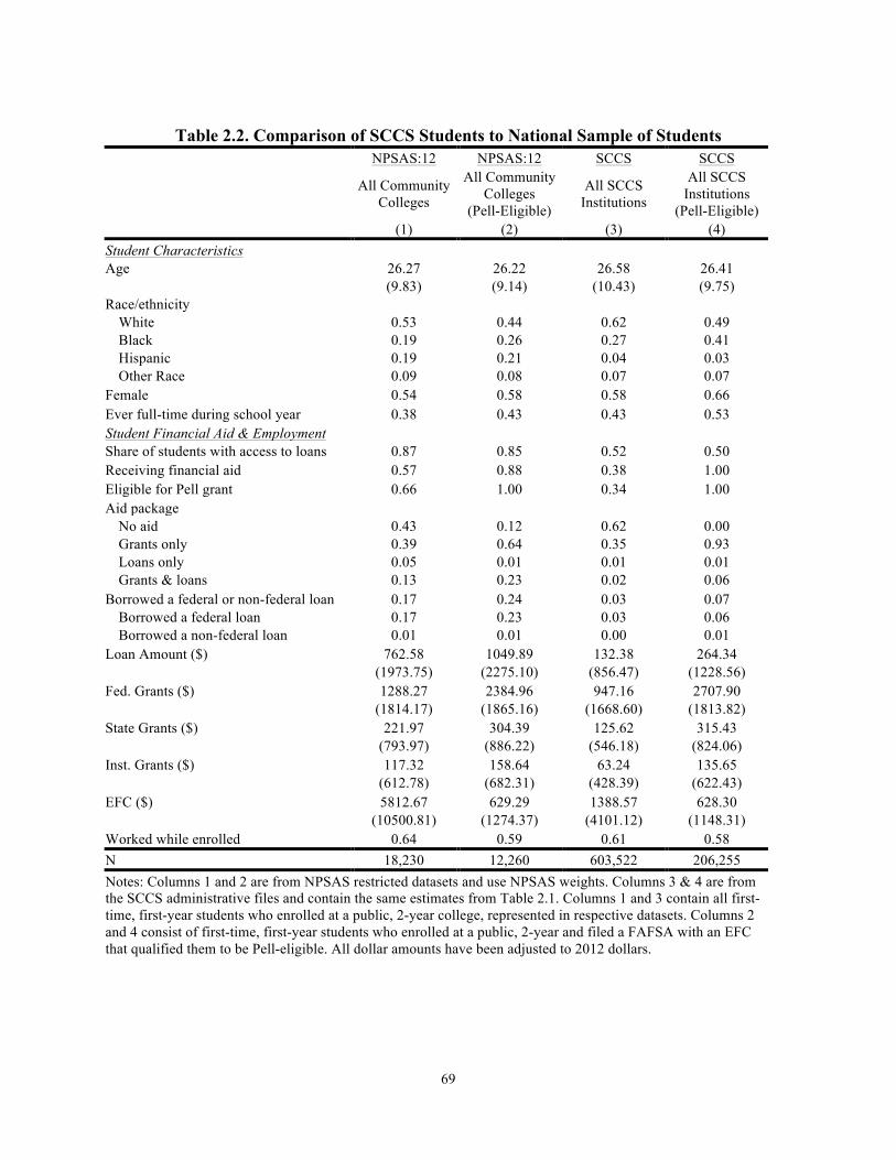
69
Table 2.2. Comparison of SCCS Students to National Sample of Students
NPSAS:12 NPSAS:12 SCCS SCCS All Community
Colleges
All Community Colleges
(Pell-Eligible)
All SCCS Institutions
All SCCS Institutions
(Pell-Eligible) (1) (2) (3) (4) Student Characteristics
Age 26.27 26.22 26.58 26.41
(9.83) (9.14) (10.43) (9.75)
Race/ethnicity White 0.53 0.44 0.62 0.49
Black 0.19 0.26 0.27 0.41 Hispanic 0.19 0.21 0.04 0.03 Other Race 0.09 0.08 0.07 0.07
Female 0.54 0.58 0.58 0.66 Ever full-time during school year 0.38 0.43 0.43 0.53 Student Financial Aid & Employment
Share of students with access to loans 0.87 0.85 0.52 0.50 Receiving financial aid 0.57 0.88 0.38 1.00 Eligible for Pell grant 0.66 1.00 0.34 1.00 Aid package
No aid 0.43 0.12 0.62 0.00 Grants only 0.39 0.64 0.35 0.93 Loans only 0.05 0.01 0.01 0.01 Grants & loans 0.13 0.23 0.02 0.06
Borrowed a federal or non-federal loan 0.17 0.24 0.03 0.07 Borrowed a federal loan 0.17 0.23 0.03 0.06 Borrowed a non-federal loan 0.01 0.01 0.00 0.01 Loan Amount ($) 762.58 1049.89 132.38 264.34
(1973.75) (2275.10) (856.47) (1228.56)
Fed. Grants ($) 1288.27 2384.96 947.16 2707.90
(1814.17) (1865.16) (1668.60) (1813.82)
State Grants ($) 221.97 304.39 125.62 315.43
(793.97) (886.22) (546.18) (824.06)
Inst. Grants ($) 117.32 158.64 63.24 135.65
(612.78) (682.31) (428.39) (622.43)
EFC ($) 5812.67 629.29 1388.57 628.30
(10500.81) (1274.37) (4101.12) (1148.31)
Worked while enrolled 0.64 0.59 0.61 0.58 N 18,230 12,260 603,522 206,255 Notes: Columns 1 and 2 are from NPSAS restricted datasets and use NPSAS weights. Columns 3 & 4 are from the SCCS administrative files and contain the same estimates from Table 2.1. Columns 1 and 3 contain all first-time, first-year students who enrolled at a public, 2-year college, represented in respective datasets. Columns 2 and 4 consist of first-time, first-year students who enrolled at a public, 2-year and filed a FAFSA with an EFC that qualified them to be Pell-eligible. All dollar amounts have been adjusted to 2012 dollars.
70
population in the state is African American, compared to 13.2 percent nationwide.25 The state’s
median household income in 2013 was approximately $46,000, whereas the national median
household income was close to $53,000.
Given that the average EFC is lower, Pell-eligible SCCS students (column 4) receive, on
average, a higher amount of federal grant aid than Pell-eligible students in the national sample
(column 2). For state and institutional aid, the amounts are fairly similar for Pell-eligible
students. Due to SCCS colleges’ lower rate of participation in the federal loan program and the
high share of Pell-eligible students receiving grant aid, the share of students with access to
federal loans and incurring debt is substantially lower than national estimates. The dollar amount
of loans that SCCS students borrow is also less.
2.6. Empirical Strategy My identification strategy exploits the variation in student loan policies within the same
community college over time. This involves using college fixed effects to estimate the within-
college difference in student outcomes before and after the college opted out the federal loan
program. The before and after difference in student outcomes at the 15 community colleges
opting out of federal loan programs is compared with the before and after difference in student
outcomes at community colleges that did not change their loan policy, resulting in what is
essentially a multi-period difference-in-difference analysis.
In the first part of my analysis, I use the following reduced form equation to examine
whether there are differences in aid amounts between the periods when institutions offer loans
and not offering loans. I also explore whether there are differences in students’ working while
enrolled.
25 Census estimates were retrieved from http://quickfacts.census.gov/qfd/index.html.
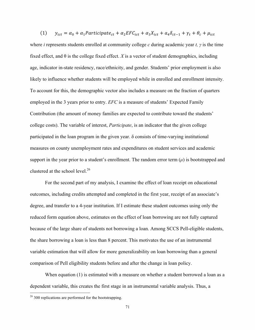
71
1 !!!!!!!!!"# = !! + !!!"#$%&%'"$(!" + !!!"#!"# + !!!!"# + !!!!"!! + !! + !! + !!"#
where i represents students enrolled at community college c during academic year t, γ is the time
fixed effect, and θ is the college fixed effect. X is a vector of student demographics, including
age, indicator in-state residency, race/ethnicity, and gender. Students’ prior employment is also
likely to influence whether students will be employed while in enrolled and enrollment intensity.
To account for this, the demographic vector also includes a measure on the fraction of quarters
employed in the 3 years prior to entry. EFC is a measure of students’ Expected Family
Contribution (the amount of money families are expected to contribute toward the students’
college costs). The variable of interest, Participate, is an indicator that the given college
participated in the loan program in the given year. δ consists of time-varying institutional
measures on county unemployment rates and expenditures on student services and academic
support in the year prior to a student’s enrollment. The random error term (µ) is bootstrapped and
clustered at the school level.26
For the second part of my analysis, I examine the effect of loan receipt on educational
outcomes, including credits attempted and completed in the first year, receipt of an associate’s
degree, and transfer to a 4-year institution. If I estimate these student outcomes using only the
reduced form equation above, estimates on the effect of loan borrowing are not fully captured
because of the large share of students not borrowing a loan. Among SCCS Pell-eligible students,
the share borrowing a loan is less than 8 percent. This motivates the use of an instrumental
variable estimation that will allow for more generalizability on loan borrowing than a general
comparison of Pell eligibility students before and after the change in loan policy.
When equation (1) is estimated with a measure on whether a student borrowed a loan as a
dependent variable, this creates the first stage in an instrumental variable analysis. Thus, a 26 300 replications are performed for the bootstrapping.
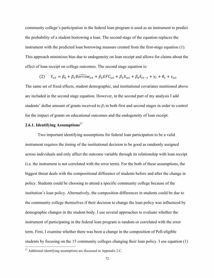
72
community college’s participation in the federal loan program is used as an instrument to predict
the probability of a student borrowing a loan. The second stage of the equation replaces the
instrument with the predicted loan borrowing measure created from the first-stage equation (1).
This approach minimizes bias due to endogeneity on loan receipt and allows for claims about the
effect of loan receipt on college outcomes. The second stage equation is:
!!(2)!!!!!!!!"# = !! + !!!"##"$!"# + !!!"#!"# + !!!!"! + !!!!"!! + !! + !! + !!"#
The same set of fixed effects, student demographic, and institutional covariates mentioned above
are included in the second stage equation. However, in the second part of my analysis I add
students’ dollar amount of grants received to β3 in both first and second stages in order to control
for the impact of grants on educational outcomes and the endogeneity of loan receipt.
2.6.1. Identifying Assumptions27 Two important identifying assumptions for federal loan participation to be a valid
instrument requires the timing of the institutional decision to be good as randomly assigned
across individuals and only affect the outcome variable through its relationship with loan receipt
(i.e. the instrument is not correlated with the error term). For the both of these assumptions, the
biggest threat deals with the compositional difference of students before and after the change in
policy. Students could be choosing to attend a specific community college because of the
institution’s loan policy. Alternatively, the composition differences in students could be due to
the community college themselves if their decision to change the loan policy was influenced by
demographic changes in the student body. I use several approaches to evaluate whether the
instrument of participating in the federal loan program is random or correlated with the error
term. First, I examine whether there was been a change in the composition of Pell-eligible
students by focusing on the 15 community colleges changing their loan policy. I use equation (1) 27 Additional identifying assumptions are discussed in Appendix 2.C.

73
to compare students with and without loan access within an institution across various
demographic and pre-college variables. Second, I examine whether or not students are likely to
attend the closest community college. Third, I determine whether there has been a change in
enrollment rates for first-time students after the change in loan policy.
Table 2.3 provides estimates for the differences in student demographics and pre-college
variables by loan availability. These student-level variables include age, gender, race/ethnicity,
distance from high school to community college, limited English proficiency, parental status,
homemaker status, academic disadvantages, disability, employment status in the quarter prior to
the first semester of enrollment, and Expected Family Contribution (EFC). Each row in Table 2.3
represents a separate regression of each variable on students’ loan access with fixed effects for
institution and year. The mean and standard deviation for each variable for students who do not
have access to loans is reported in column 2 and the sample size is provided in column 3.
When considering all estimates as a whole, there are no apparent demographic
differences between students who do not have loan access and those who do. There are, however,
several differences worth discussing, with regards to age, Black and Hispanic students, and
disability status. While these differences are significant, the magnitudes of these differences are
small and thus unlikely to cause serious bias in the estimates. For example, students with loan
access are 1.9 percentage points less likely to be Black. While this difference is significant at the
5 percent level, this difference is small when considering the large share of students who are
Black, comprising of 43 percent of the sample.

74
Table 2.3. Differences in Pre-College Variables by Loan Access
Participate Control Mean Sample Size (1) (2) (3) Age at entry -0.615* 26.557 47,683
(0.343) [9.778]
Female -0.009 0.671 47,683
(0.013) [0.470]
White 0.019 0.437 47,683
(0.014) [0.496]
Black -0.019** 0.433 47,683
(0.009) [0.496]
Hispanic 0.004** 0.017 47,683
(0.002) [0.130]
Other Race -0.004 0.112 47,683
(0.014) [0.316]
Distance to community college (miles) -0.675 17.201 34,474
(1.152) [29.802]
In-state Resident 0.004 0.932 47,683
(0.006) [0.252]
Limited English Proficiency 0.001 0.003 47,683
(0.001) [0.058]
Single Parent -0.014 0.070 47,683
(0.016) [0.255]
Homemaker -0.003 0.039 47,683
(0.008) [0.194]
Academically Disadvantaged 0.078 0.365 47,683
(0.074) [0.482]
Handicap -0.008* 0.013 47,683
(0.004) [0.113]
Employed 1quarter prior to entry 0.016 0.522 47,683
(0.013) [0.500]
Earnings 1 quarter prior to entry -146.759 7147.441 47,683
(482.299) [9765.362]
EFC at entry 18.398 503.013 47,683
(28.011) [985.208]
Notes: Each row represents a separate regression of each variable on whether the student has loan access. Standard errors are in parentheses and are clustered at the institution level. The variable mean and standard deviation (in brackets) for students with loan access is reported in column 2 and the sample size for the regression is provided in column 3. Distance to community college is measured in miles and is the distance between students’ high school and community college. Distance to college is only available for students who reported a high school to the community college. *** <0.01 **<0.05 *<0.10
75
Measuring the distance between students’ primary home and community college can also
help determine whether Pell-eligible students are choosing to attend a specific college based on
loan policy. Table 2.3 illustrates that the difference in distance from students’ high school to
community college is not statistically significant. But it is worth noting the geographic location
of SCCS community colleges in relation to one another and their loan policy. Geographically,
the 15 community colleges observed as having opted out of the Stafford loan program are evenly
distributed throughout the state.28 Unique to SCCS is that no two community colleges reside
within the same county. These 15 community colleges, and their respective counties, are often
surrounded by, or close to, a county containing a community college that never changes their
loan policy (either because it always participated or never participated). However, the majority
of students still attend the closest community college. For example, for the 15 community
college, roughly 77 percent of financial aid recipients attended a community college that was
closest to their home; 13 percent attended a community college in a neighboring county, and; 10
percent of the sample attended a community college that was deemed a far distance.29
Regressions were estimated to determine if there was a difference in students attending the
closest college or college deemed to be a far distance. The results indicated that there were no
significant differences between students who do not have loan access and those who do.30
One important threat that could make the instrument of loan participation invalid deals
with the change in loan policy possibly influencing community colleges’ enrollment rates.
Alternatively, a community college’s change in loan policy could have happened in conjunction
28 A map of SCCS college is provided in Figure 2.8 in Appendix 2.D. 29 Figure 2.9 in Appendix 2.D illustrates whether students are traveling far distances to attend one of the 15 community colleges. The share of students attending a community college not closest to home or outside of the community college service district does not appear to change relative to the change in loan policy. 30 Results from these regressions indicate that the difference were -0.003 (0.020) for attendance to closest community college and -0.004 (0.012) for attendance to community college in neighboring county or farther.
76
with or prior to another institutional decision that increased the college’s classroom capacity,
such as opening a new building. To determine whether enrollment rates are correlated with the
timing of the loan policy change for the 15 community colleges, I used data from the Integrated
Postsecondary Education Data System (IPEDS) (2014e) to examine whether there was a
significant difference in the share of the student body attending for the first-time before and after
the change in loan policy. In the first five years after the switch in loan policy, only 4 out of the
15 community colleges increased the share of first-time of students by an average of 5 percent
per year.31 To determine whether these enrollment changes are significant, I used equation 1
without student and institutional controls and the share of first-time students as the dependent
variable. Results from the fixed effects regression were highly insignificant and suggest that the
change in loan policy did not influence enrollment rates.32
Another identifying assumption requires there to be a nonzero relationship between the
instrument (federal loan participation) and the endogenous treatment variable (loan receipt).
Researchers often gauge the strength of the relationship between the two variables from the first
stage F-statistics. Since my regression models cluster the standard errors at the college level, I
employ the Kleibergen-Paap Wald test. The F-statistic from the first stage is 23.20, which
exceeds the rule-of-thumb value of 10 (Staiger & Stock, 1997) and the maximal value of 16.36
proposed by Stock and Yogo (2005). Because the F-statistic from the first stage exceeds
recommended levels, the instrument on federal loan participation does not violate this
assumption.
31 Figure 2.10 in Appendix 2.D displays the share of students enrolling for the first time before and after the switching in loan policy for the 15 community colleges. 32 Results from this regression indicate that the difference was -0.015 (0.014).

77
2.7. Results 2.7.1. Main Results
Table 2.4 presents the results for the first part of my analysis examining the effects of
federal loan participation on financial aid and employment. Each panel contains results for
separate topical outcomes: panel A examines student loans, panel B for grants, and panel F for
employment while enrolled. In addition to examining all grant programs in panel B, I also
examine the differences in grant receipt and amounts for federal (panel C), state (panel D), and
institutional grant programs (panel E). Columns 1 and 3 only include academic year and college
fixed effects. Columns 2 and 4 add student demographic controls and time-varying community
college measures. The standard errors are provided below each coefficient (cluster bootstrapped
at the college level), followed by the mean of the dependent variable for students without access
to loans (attend a community college that opted out of the federal loan program at the time of
enrollment).
As the results in Panel A in Table 2.4 illustrate, Pell-eligible students who attend an
institution that is participating in the federal loan program are 7.6 percentage points more likely
to borrow than students with no such access. Also, having federal loan access significantly
increases overall borrowing by $368 a year, or $4,837 ($367.61/0.076) among the 7.6 percent
who take loans. This effect is large, considering the average SCCS student borrows $132 in the
first year ($4,400 among the 3 percent who take loans).
Results in panel B suggest that Pell-eligible students enrolling when a community college
participates in the federal loan program are less likely to receive grant aid (combination of
federal, state, and institution). Estimates indicated that the share of Pell-eligible students
receiving grant aid decreased by less than 1 percent before community colleges opted out of the
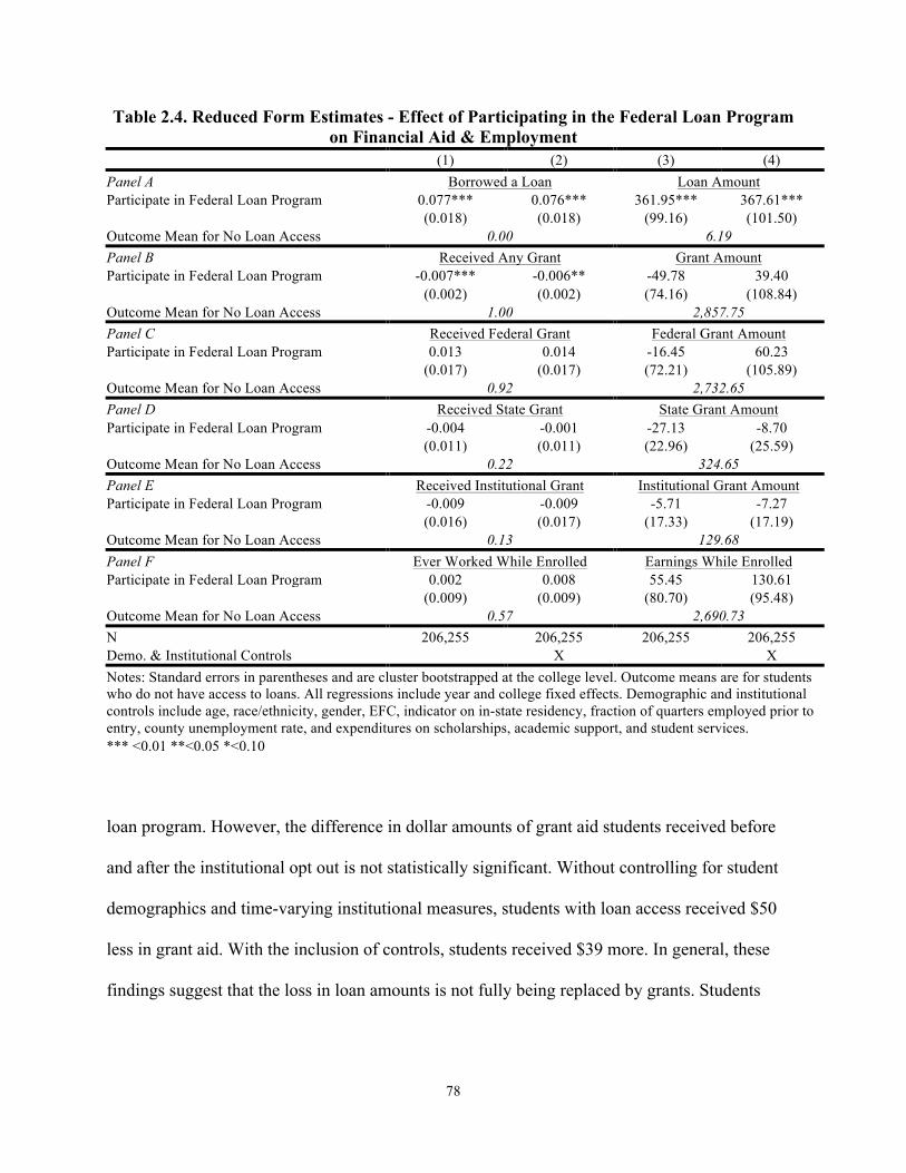
78
Table 2.4. Reduced Form Estimates - Effect of Participating in the Federal Loan Program on Financial Aid & Employment
(1) (2) (3) (4) Panel A Borrowed a Loan Loan Amount Participate in Federal Loan Program 0.077*** 0.076*** 361.95*** 367.61***
(0.018) (0.018) (99.16) (101.50)
Outcome Mean for No Loan Access 0.00 6.19 Panel B Received Any Grant Grant Amount Participate in Federal Loan Program -0.007*** -0.006** -49.78 39.40
(0.002) (0.002) (74.16) (108.84)
Outcome Mean for No Loan Access 1.00 2,857.75 Panel C Received Federal Grant Federal Grant Amount Participate in Federal Loan Program 0.013 0.014 -16.45 60.23
(0.017) (0.017) (72.21) (105.89)
Outcome Mean for No Loan Access 0.92 2,732.65 Panel D Received State Grant State Grant Amount Participate in Federal Loan Program -0.004 -0.001 -27.13 -8.70
(0.011) (0.011) (22.96) (25.59)
Outcome Mean for No Loan Access 0.22 324.65 Panel E Received Institutional Grant Institutional Grant Amount Participate in Federal Loan Program -0.009 -0.009 -5.71 -7.27
(0.016) (0.017) (17.33) (17.19)
Outcome Mean for No Loan Access 0.13 129.68 Panel F Ever Worked While Enrolled Earnings While Enrolled Participate in Federal Loan Program 0.002 0.008 55.45 130.61
(0.009) (0.009) (80.70) (95.48)
Outcome Mean for No Loan Access 0.57 2,690.73 N 206,255 206,255 206,255 206,255 Demo. & Institutional Controls
X
X
Notes: Standard errors in parentheses and are cluster bootstrapped at the college level. Outcome means are for students who do not have access to loans. All regressions include year and college fixed effects. Demographic and institutional controls include age, race/ethnicity, gender, EFC, indicator on in-state residency, fraction of quarters employed prior to entry, county unemployment rate, and expenditures on scholarships, academic support, and student services. *** <0.01 **<0.05 *<0.10
loan program. However, the difference in dollar amounts of grant aid students received before
and after the institutional opt out is not statistically significant. Without controlling for student
demographics and time-varying institutional measures, students with loan access received $50
less in grant aid. With the inclusion of controls, students received $39 more. In general, these
findings suggest that the loss in loan amounts is not fully being replaced by grants. Students
79
enrolling after an institution opted out lost the ability to borrow as much as $368 and lost an
average of $39 through the combination of federal, state, and institution grant aid programs.
Table 2.4 also displays whether there was a difference before and after the switch in loan
policy for federal (panel C), state (panel D), and institutional (panel E) grant aid programs. The
results are not statistically significant for any of the three grant aid programs. I do, however, find
that Pell-eligible students with loan access were 1 percentage point more likely to obtain a
federal grant and received $60 more than Pell-eligible students without loan access. For state and
institution grant programs, the findings show a similar pattern: Pell-eligible students with loan
access were less likely to receive grant aid (less than 1 percentage point) and the dollar amount
was smaller by $7 and $9.
Regarding the relationship between access to federal loans and employment, the results
indicate that colleges’ loan policy has a positive influence on Pell-eligible students’ employment
decisions while enrolled in school, but the results are not statistically significant. Students having
access to loans were less than 1 percent more likely to work and earned $131 more while
enrolled. Taking aside the statistical insignificance of the results, the positive findings associated
with loan access are still surprising. One would expect that students without loan access would
be more likely to work. But the findings on employment are consistent with previous research.
Boushey (2005) found that 84 percent of undergraduates who had loans at four year institutions,
be it not-for-profit or public, had a job while enrolled, compared to 67 percent of undergraduates
with no loans at not-for-profit colleges and 78 percent of undergraduates without loans at public
colleges.
Next, I investigate the effect of participating in the Stafford loan program and loan
borrowing on Pell-eligible students’ enrollment intensity. The following results come from the
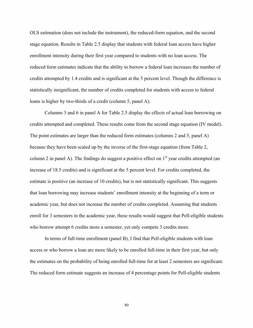
80
OLS estimation (does not include the instrument), the reduced-form equation, and the second
stage equation. Results in Table 2.5 display that students with federal loan access have higher
enrollment intensity during their first year compared to students with no loan access. The
reduced form estimates indicate that the ability to borrow a federal loan increases the number of
credits attempted by 1.4 credits and is significant at the 5 percent level. Though the difference is
statistically insignificant, the number of credits completed for students with access to federal
loans is higher by two-thirds of a credit (column 5, panel A).
Columns 3 and 6 in panel A for Table 2.5 display the effects of actual loan borrowing on
credits attempted and completed. These results come from the second stage equation (IV model).
The point estimates are larger than the reduced form estimates (columns 2 and 5, panel A)
because they have been scaled up by the inverse of the first-stage equation (from Table 2,
column 2 in panel A). The findings do suggest a positive effect on 1st year credits attempted (an
increase of 18.5 credits) and is significant at the 5 percent level. For credits completed, the
estimate is positive (an increase of 10 credits), but is not statistically significant. This suggests
that loan borrowing may increase students’ enrollment intensity at the beginning of a term or
academic year, but does not increase the number of credits completed. Assuming that students
enroll for 3 semesters in the academic year, these results would suggest that Pell-eligible students
who borrow attempt 6 credits more a semester, yet only compete 3 credits more.
In terms of full-time enrollment (panel B), I find that Pell-eligible students with loan
access or who borrow a loan are more likely to be enrolled full-time in their first year, but only
the estimates on the probability of being enrolled full-time for at least 2 semesters are significant.
The reduced form estimate suggests an increase of 4 percentage points for Pell-eligible students
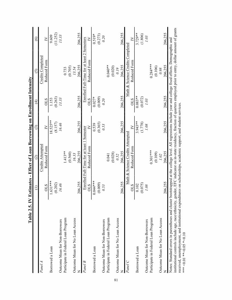
81
Tab
le 2
.5. I
V E
stim
ates
- E
ffec
t of L
oan
Bor
row
ing
on E
nrol
lmen
t Int
ensi
ty
(1
) (2
) (3
)
(4)
(5)
(6)
Pane
l A
Cre
dits
Atte
mpt
ed
C
redi
ts C
ompl
eted
O
LS
Red
uced
For
m
IV
O
LS
Red
uced
For
m
IV
Bor
row
ed a
Loa
n 1.
631*
**
18
.525
**
1.
153
9.
609
(0
.202
)
(8.1
57)
(0
.263
)
(11.
252)
O
utco
me
Mea
n fo
r Non
-Bor
row
ers
16.4
6
16.4
6
13.3
3
13.3
3 Pa
rtici
pate
in F
eder
al L
oan
Prog
ram
1.41
3**
0.
733
(0
.560
)
(0.7
05)
O
utco
me
Mea
n fo
r No
Loan
Acc
ess
16
.33
13
.54
N
20
6,25
5 20
6,25
5 20
6,25
5
206,
255
206,
255
206,
255
Pane
l B
Enro
lled
Full-
Tim
e fo
r at l
east
1 S
emes
ter
En
rolle
d Fu
ll-Ti
me
for a
t lea
st 2
Sem
este
rs
O
LS
Red
uced
For
m
IV
O
LS
Red
uced
For
m
IV
Bor
row
ed a
Loa
n 0.
044*
**
0.
539
0.
027*
0.51
9*
(0
.009
)
(0.3
65)
(0
.009
)
(0.2
73)
Out
com
e M
ean
for N
on-B
orro
wer
s 0.
53
0.
53
0.
20
0.
20
Parti
cipa
te in
Fed
eral
Loa
n Pr
ogra
m
0.
041
0.
040*
*
(0.0
28)
(0
.020
)
Out
com
e M
ean
for N
o Lo
an A
cces
s
0.52
0.19
N
206,
255
206,
255
206,
255
20
6,25
5 20
6,25
5 20
6,25
5 Pa
nel C
M
ath
& S
cien
ce C
redi
ts A
ttem
pted
Mat
h &
Sci
ence
Cre
dits
Com
plet
ed
O
LS
Red
uced
For
m
IV
O
LS
Red
uced
For
m
IV
Bor
row
ed a
Loa
n 0.
102
3.
943*
*
0.08
3**
3.
729*
*
(0
.075
)
(1.7
78)
(0
.072
)
(1.8
06)
Out
com
e M
ean
for N
on-B
orro
wer
s 1.
08
1.
08
1.
03
1.
03
Parti
cipa
te in
Fed
eral
Loa
n Pr
ogra
m
0.
301*
**
0.
284*
**
(0
.109
)
(0.1
06)
O
utco
me
Mea
n fo
r No
Loan
Acc
ess
1.
02
0.
98
N
20
6,25
5 20
6,25
5 20
6,25
5
206,
255
206,
255
206,
255
Not
es: S
tand
ard
erro
rs in
par
enth
eses
and
clu
ster
boo
tstra
pped
at t
he c
olle
ge le
vel.
All
regr
essi
ons i
nclu
de y
ear a
nd c
olle
ge fi
xed
effe
cts.
Dem
ogra
phic
and
in
stitu
tiona
l con
trols
incl
ude
age,
race
/eth
nici
ty, g
ende
r, EF
C in
dica
tor o
n in
-sta
te re
side
ncy,
frac
tion
of q
uarte
rs e
mpl
oyed
prio
r to
entry
, dol
lar a
mou
nt o
f gra
nts
rece
ived
, une
mpl
oym
ent,
and
inst
itutio
nal e
xpen
ditu
res o
n sc
hola
rshi
ps, a
cade
mic
supp
ort,
and
stud
ent s
ervi
ces.
**
* <0
.01
**<0
.05
*<0.
10
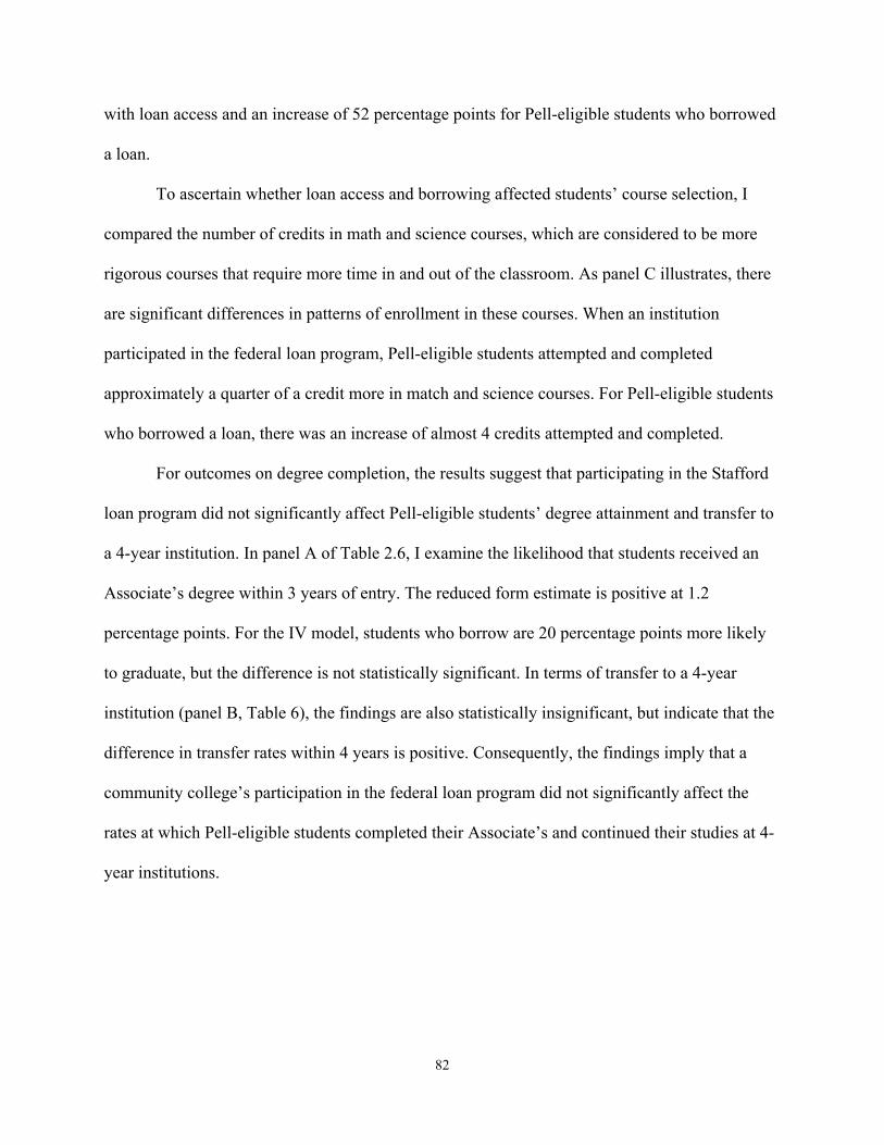
82
with loan access and an increase of 52 percentage points for Pell-eligible students who borrowed
a loan.
To ascertain whether loan access and borrowing affected students’ course selection, I
compared the number of credits in math and science courses, which are considered to be more
rigorous courses that require more time in and out of the classroom. As panel C illustrates, there
are significant differences in patterns of enrollment in these courses. When an institution
participated in the federal loan program, Pell-eligible students attempted and completed
approximately a quarter of a credit more in match and science courses. For Pell-eligible students
who borrowed a loan, there was an increase of almost 4 credits attempted and completed.
For outcomes on degree completion, the results suggest that participating in the Stafford
loan program did not significantly affect Pell-eligible students’ degree attainment and transfer to
a 4-year institution. In panel A of Table 2.6, I examine the likelihood that students received an
Associate’s degree within 3 years of entry. The reduced form estimate is positive at 1.2
percentage points. For the IV model, students who borrow are 20 percentage points more likely
to graduate, but the difference is not statistically significant. In terms of transfer to a 4-year
institution (panel B, Table 6), the findings are also statistically insignificant, but indicate that the
difference in transfer rates within 4 years is positive. Consequently, the findings imply that a
community college’s participation in the federal loan program did not significantly affect the
rates at which Pell-eligible students completed their Associate’s and continued their studies at 4-
year institutions.

83
Table 2.6. IV Estimates - Effect of Loan Borrowing on College Completion (1) (2) (3) Panel A Obtain AA with 3 years of entry OLS Reduced Form IV Borrowed a Loan 0.001
0.204
(0.005)
(0.167)
Outcome Mean for Non-Borrowers 0.09
0.09 Participate in Federal Loan Program
0.012
(0.008) Outcome Mean for No Loan Access
0.08
N 132,147 132,147 132,147 Panel B Transfer to 4yr within 4 years of entry
OLS Reduced Form IV
Borrowed a Loan 0.061
0.038
(0.007)
(0.166)
Outcome Mean for Non-Borrowers 0.20
0.20 Participate in Federal Loan Program
0.002
(0.008) Outcome Mean for No Loan Access
0.19
N 138,017 138,017 138,017 Notes: See notes in Table 2.5. Samples consist of Pell-eligible students who enrolled before the 2007-08 academic year. *** <0.01 **<0.05 *<0.10 2.7.2. Results by Subgroups
A change in loan policy is likely to differentially affect subgroups of students. For
example, traditionally aged students (less than 24 years of age) are likely to have different
educational goals than non-traditional students (over 25 years of age) (Cohen & Brawer, 2008).
Also, students have different levels of financial constraints, as some are likely to receive
financial support from family members and will have a lower level of financial need. In Table
2.7, I examine outcomes across subgroups and employ the same model specifications as above
on each group – students less than 24 years of age, older than 24 years of age, White, Black,
male, and female. Column 1 in Table 2.7 contains the same coefficients from columns 2 and 4 in
Table 2.4, columns 3 and 6 in Table 2.5, and column 3 in Table 2.6. Panel A consists of the
reduced form estimates on financial aid and panel B consists of the IV estimates on enrollment
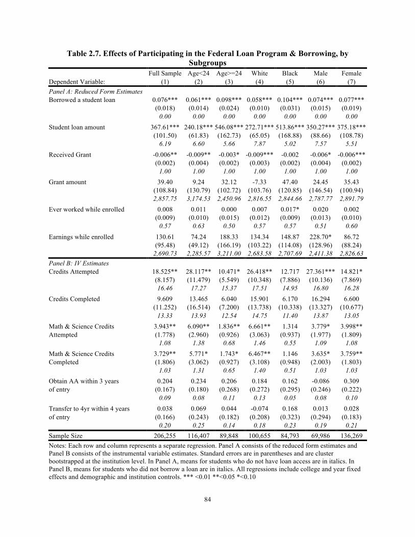
84
Table 2.7. Effects of Participating in the Federal Loan Program & Borrowing, by Subgroups
Full Sample Age<24 Age>=24 White Black Male Female Dependent Variable: (1) (2) (3) (4) (5) (6) (7) Panel A: Reduced Form Estimates
Borrowed a student loan 0.076*** 0.061*** 0.098*** 0.058*** 0.104*** 0.074*** 0.077***
(0.018) (0.014) (0.024) (0.010) (0.031) (0.015) (0.019)
0.00 0.00 0.00 0.00 0.00 0.00 0.00
Student loan amount 367.61*** 240.18*** 546.08*** 272.71*** 513.86*** 350.27*** 375.18***
(101.50) (61.83) (162.73) (65.05) (168.88) (88.66) (108.78)
6.19 6.60 5.66 7.87 5.02 7.57 5.51
Received Grant -0.006** -0.009** -0.003* -0.009*** -0.002 -0.006* -0.006***
(0.002) (0.004) (0.002) (0.003) (0.002) (0.004) (0.002)
1.00 1.00 1.00 1.00 1.00 1.00 1.00
Grant amount 39.40 9.24 32.12 -7.33 47.40 24.45 35.43
(108.84) (130.79) (102.72) (103.76) (120.85) (146.54) (100.94)
2,857.75 3,174.53 2,450.96 2,816.55 2,844.66 2,787.77 2,891.79
Ever worked while enrolled 0.008 0.011 0.000 0.007 0.017* 0.020 0.002
(0.009) (0.010) (0.015) (0.012) (0.009) (0.013) (0.010)
0.57 0.63 0.50 0.57 0.57 0.51 0.60
Earnings while enrolled 130.61 74.24 188.33 134.34 148.87 228.70* 86.72
(95.48) (49.12) (166.19) (103.22) (114.08) (128.96) (88.24)
2,690.73 2,285.57 3,211.00 2,683.58 2,707.69 2,411.38 2,826.63
Panel B: IV Estimates Credits Attempted 18.525** 28.117** 10.471* 26.418** 12.717 27.361*** 14.821*
(8.157) (11.479) (5.549) (10.348) (7.886) (10.136) (7.869)
16.46 17.27 15.37 17.51 14.95 16.80 16.28
Credits Completed 9.609 13.465 6.040 15.901 6.170 16.294 6.600
(11.252) (16.514) (7.200) (13.738) (10.338) (13.327) (10.677)
13.33 13.93 12.54 14.75 11.40 13.87 13.05
Math & Science Credits 3.943** 6.090** 1.836** 6.661** 1.314 3.779* 3.998** Attempted (1.778) (2.960) (0.926) (3.063) (0.937) (1.977) (1.809)
1.08 1.38 0.68 1.46 0.55 1.09 1.08
Math & Science Credits 3.729** 5.771* 1.743* 6.467** 1.146 3.635* 3.759** Completed (1.806) (3.062) (0.927) (3.108) (0.948) (2.003) (1.803)
1.03 1.31 0.65 1.40 0.51 1.03 1.03
Obtain AA within 3 years 0.204 0.234 0.206 0.184 0.162 -0.086 0.309 of entry (0.167) (0.180) (0.268) (0.272) (0.295) (0.246) (0.222)
0.09 0.08 0.11 0.13 0.05 0.08 0.10
Transfer to 4yr within 4 years 0.038 0.069 0.044 -0.074 0.168 0.013 0.028 of entry (0.166) (0.243) (0.182) (0.208) (0.323) (0.294) (0.183)
0.20 0.25 0.14 0.18 0.23 0.19 0.21
Sample Size 206,255 116,407 89,848 100,655 84,793 69,986 136,269 Notes: Each row and column represents a separate regression. Panel A consists of the reduced form estimates and Panel B consists of the instrumental variable estimates. Standard errors are in parentheses and are cluster bootstrapped at the institution level. In Panel A, means for students who do not have loan access are in italics. In Panel B, means for students who did not borrow a loan are in italics. All regressions include college and year fixed effects and demographic and institution controls. *** <0.01 **<0.05 *<0.10
85
intensity and degree completion. The standard errors appear below each coefficient, cluster
bootstrapped at the college level; the means of the dependent variable for students who did not
have access to loans (in panel A) or did not borrow (in panel B) are in italics.
Similar to previous results, I find that access to Stafford loans significantly increases Pell-
eligible students’ likelihood of borrowing and their loan amounts across all subgroups. While the
results form the entire analytic sample showed a 7.6 percentage point increase in borrowing and
a $368 increase in loan amounts, the difference in borrowing and loan amounts is even larger for
particular subgroups. For non-traditional students, access to federal loans is associated with a 10-
percentage point increase in borrowing and the loan amount increases $546. For Black students,
participation in federal loans increased loan amounts by $514.
Across all subgroups, the share of Pell-eligible students enrolling before the community
college opted out were less likely to receive a grant, yet the dollar amount of grants they receive
is higher than students without loan access. The only group that received less grant aid before the
switch in loan policy was white Pell-eligible students. For Black students, the before and after
difference in the share of students receiving a grant is statistically insignificant. However, Black
students with loan access were 1.7 percentage points more likely to work while enrolled, an
estimate that is significant at the 10 percent level.
Though estimates from Table 2.5 showed that Pell-eligible students who borrow a loan
attempted more credits in their first year, disaggregating results by subgroups reveals the
estimated differences in credits attempted is even larger for particular subgroups. For example,
for students younger than 24 years old, the difference is 28 credits. The difference in credits
completed is also positive across all subgroups, but statistically insignificant. For attempted and
completed math and science credits, the results are positive across subgroups, and, except for
86
Black students, is statistically significant at the 5 or 10 percent level. Similar to the results in
Table 2.6, the share of Pell-eligible students obtaining an Associate’s within 3 years of entry and
transfer to a 4-year college within 4-years of entry is statistically insignificant across subgroups.
However, the results indicate that the difference is negative for particular subgroups. For
example, male students borrowing a loan were 8.6 percentage points less likely to receive an
Associate’s. White students who borrow were 7.4 percentage points less likely to transfer to a 4-
year institution.
2.7.3. Robustness Check One concern with the main results is the sample includes only students who were eligible
for a Pell-grant. Limiting the sample to this particular sample hinders the ability to make
inferences for SCCS system as a whole. For my first robustness check, I run my estimations
again using the full sample of financial aid recipients, which also includes students who were
ineligible for a Pell grant.
The results in Table 2.8 are similar to the main results presented in Table 2.4. Access to
loans increases the probability of borrowing by 9.5 percentage points and the average loan
amount increases $436 (or $4,589, conditional on borrowing). Consistent with my previous
results, students enrolling when the community college participated in the federal loan program
were 2.4 percentage points less likely receive a grant. The average dollar amount of grants for
these students is also $22 less than students without loan access.
Panel B in Table 2.8 displays the results on enrollment intensity and degree completion.
Again, the findings are consistent with the main results. More specifically, financial aid
recipients who borrowed a loan attempted 17 more credits than non-borrowers, with the
difference being significant at the 1 percent level. The difference in credits completed is also
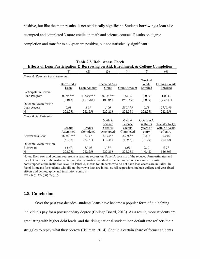
87
positive, but like the main results, is not statistically significant. Students borrowing a loan also
attempted and completed 3 more credits in math and science courses. Results on degree
completion and transfer to a 4-year are positive, but not statistically significant.
Table 2.8. Robustness Check Effects of Loan Participation & Borrowing on Aid, Enrollment, & College Completion
(1) (2) (3) (4) (5) (6) Panel A: Reduced Form Estimates
Borrowed a Loan Loan Amount
Received Any Grant Grant Amount
Worked While
Enrolled Earnings While
Enrolled ! Participate in Federal Loan Program 0.095*** 436.07*** -0.024*** -22.03 0.009 146.43
(0.018) (107.966) (0.005) (94.189) (0.009) (93.331)
Outcome Mean for No Loan Access 0.01 8.59 1.00 2801.79 0.58 2735.49 N 222,258 222,258 222,258 222,258 222,258 222,258 Panel B: IV Estimates
Credits
Attempted Credits
Completed
Math & Science Credits
Attempted
Math & Science Credits
Completed
Obtain AA within 3 years of
entry
Transfer to 4yr within 4 years
of entry ! ! ! ! ! ! !Borrowed a Loan 16.550*** 8.777 3.173** 2.976** 0.207 0.045
(6.336) (8.781) (1.244) (1.258) (0.129) (0.122)
Outcome Mean for Non-Borrowers 16.69 13.60 1.14 1.09 0.10 0.21 N 222,258 222,258 222,258 222,258 140,423 146,863 Notes: Each row and column represents a separate regression. Panel A consists of the reduced form estimates and Panel B consists of the instrumental variable estimates. Standard errors are in parentheses and are cluster bootstrapped at the institution level. In Panel A, means for students who do not have loan access are in italics. In Panel B, means for students who did not borrow a loan are in italics. All regressions include college and year fixed effects and demographic and institution controls. *** <0.01 **<0.05 *<0.10!
! ! ! ! ! 2.8. Conclusion
Over the past two decades, students loans have become a popular form of aid helping
individuals pay for a postsecondary degree (College Board, 2013). As a result, more students are
graduating with higher debt loads, and the rising national student loan default rate reflects their
struggles to repay what they borrow (Hillman, 2014). Should a certain share of former students
88
default on their government-backed loans, the federal government sanctions these colleges and
prohibits them from providing any federal aid to currently enrolled students. In response,
colleges are restricting their students’ access to federal loan as a proactive approach to protect
their eligibility to disburse federal financial aid. The unintended consequence of this
accountability mechanism may dramatically reduce access to federal loans if the number of
institutions opting out of the program continues to increase.
The findings from this paper suggest that providing Pell-eligible students with the
opportunity to borrow has positive effects on the number of credits students’ attempt in their first
year. Loan borrowing also increases the number of credits completed, degree completion, and
transfer to a 4-year institution, although the results are not statistically significant. More
importantly, Pell-eligible students borrowing a loan are have a higher enrollment intensity in
STEM related courses, which are in alignment with occupations that are considered to be in
demand and offer higher pay in the workforce. Given the positive effects for students,
policymakers may want to consider revising accountability rules so that metrics on loan use and
default rates do not create an incentive for institutions to opt of the program and limit the ability
for students to borrow loans.
Furthermore, results from this paper suggest that colleges choosing to exclude federal
loans from students’ financial aid packages should have practices in place to help students
financially and academically. One particular federal, state, or institution aid program – or a
combination of all three – will not necessarily cover the amount of aid lost when opting out of
the federal student loan program; institutions may need to develop financial aid programs to
supplement existing grant aid. Institutions should also be aware that students might reduce their
89
enrollment intensity in the absence of loans, and they may want to have academic resources
available to ensure that students are able to complete their degree.
It is important to note that the share of SCCS students borrowing a loan is lower than
national estimates. Nationally, roughly 17 percent of community college students borrow,
compared to 3 percent at SCCS. Possible reasons provided by SCSS financial aid administrators
for the low borrowing rates are the extremely low tuition rates and a combination of aid
programs that can cover directs costs for students with extremely high need. Additionally, the
low loan take-up also reflects the high share of community colleges that prohibit students from
borrowing; only 35 percent of SCCS community colleges participated in the federal loan
program in 2009-10. These are important issues to consider when thinking about the
generalizability of these results to other contexts. More specifically, this paper is not able to fully
examine the impact of losing loan eligibility for students who are just above Pell-eligibility
threshold nor for students who attend highly priced institutions, which are two groups of students
who depend on using loans to pay for college. If the results from this paper provide any
indication, the impact of losing loan eligibility for these students may be even larger.
Though the analysis in this paper offers insight into the student-level consequences of
community colleges’ decision in whether or not to participation in the Stafford loan program,
additional research is needed surrounding institutional decisions to not participate in the federal
loan program – and on the effects of loan access more generally. At the institutional level, further
research is necessary to determine whether other factors besides the cohort default rate contribute
to institutions’ decision to opt out and how accountability mechanisms could be revised to
reduced or eliminate federal loan access (or lack thereof) on college access and educational
outcomes. Information on employment and private loan use is limited with the SCCS datasets.

90
More research needs to examine how the institutional decision not to offer federal loans lead
students to rely on working while or rely on private loans with higher interest rates and less
flexible repayment plans. The national dialogue is currently dominated with concerns over rising
debt levels, but before limiting access to loans is embraced as the solution, it is important to
understand the extent to which federal loans are contributing to the problem and the effects a
reduction in loan access would have on educational outcomes.
91
Appendix 2 Appendix 2.A. Theoretical Framework
This paper is guided by two theories that help to explain how institutional-level decisions
to opt out of the federal loan program affect student-level educational outcomes. At the
institutional level, I draw on principal-agent theory to understand why an institution would opt
out of the federal student loan program. At the student level, I utilize the time allocation strand of
human capital theory to illuminate how students’ inability to take out federal loans – resulting
from the institution’s decision to opt out – may condition their educational trajectories in ways
that affect their progress toward degree completion and other outcomes. I developed this
framework using insights from the aforementioned interviews with financial aid administrators
and it assumes that institutions do not substitute the loss of loans for another form of financial
aid created specifically to cover the loss.
2.A.1 Principal-Agent Theory
Under the principal-agent theory, an agent acts on behalf of, or carries out a designed task
for, the principal (Macho-Stadler & Perez-Castrillo, 2001; Milgrom & Roberts, 1992). The
relationship between the two parties is “governed by a contract specifying what the agent should
do and what the principal must do in return” (Perrow, 1986, p. 224). This theory assumes that the
principal designs the contract and then offers it to the agent, who then decides whether or not to
accept the terms of the contract. Once the agent agrees to the contract, the agent is to carry out
92
the actions as specified in the contract and is expected to work in the best interests of the
principal.
In the case of community colleges and the federal loan program, the federal government
is the principal. The government created the loan program to increase college access and
completion by providing students with the financial assistance to make college affordable. The
government entrusted administration of the loans to the educational institutions – the agents –
and relies on the colleges to disburse the aid in a manner that furthers the goals of the program.
The program guidelines – the contract – stipulate the requirements to which colleges must adhere
and the mechanisms by which the federal government monitors colleges’ participation.
According to principal-agent theory, however, problems can arise after the parties have
agreed upon the terms of the contract. Because agents are trying to maximize their own utility,
they sometimes make decisions that are pursuant to their own interests rather than the
principal’s. This misalignment is referred to as “shirking” (Lane, 2012). To prevent shirking, the
principal can use incentives or penalties to ensure that the agent acts according to the principal’s
goals (Laffont & Martimort, 2002). As mentioned previously, one mechanism that the U.S.
Department of Education utilizes is the cohort default rate. If a college’s default rate exceeds 30
or 40 percent, the college is sanctioned by the federal government and prohibited from
participating in federal financial aid programs. Since it is in the best interests of community
colleges to avoid having a CDR that threatens their ability to provide students with federal grants
such as the Pell, this policy was implemented to ensure that community colleges administer loans
in a manner that furthers the goals of the program.
As the principal-agent theory highlights, however, if the incentives or penalties are
ambiguous or do not align with the contracted goals, a disconnect can arise and lead to further
93
shirking by agents (Laffont & Martimort, 2002). The CDR threshold and penalties create –
perhaps inadvertently – an incentive for community colleges to opt out of the federal loan
program entirely in order to maintain eligibility for other federal aid programs. Doing so protects
the interests of the community colleges, but detracts from the federal government’s efforts to
provide financial aid to increase college access and completion. Lack of access to loans may
prolong time to degree completion or increase dropout rates, and directing students to private
lenders can, as discussed earlier, be detrimental to students’ long-term financial situation.
2.A.2 Time Allocation
Whereas principal-agent theory offers insight into why colleges choose to opt out of the
federal loan program, human capital theory and time allocation help explain the effects of this
decision on students’ educational outcomes. Human capital theory is the most common approach
employed by higher education researchers to analyze students’ decision-making behavior in
relation to college enrollment, completion, and financing (Long, 2007; Paulsen & Toutkoushian,
2008). Attending college is viewed as an investment in one’s human capital because it generally
increases individuals’ productive capacities and provides them with pecuniary and nonpecuniary
benefits (Becker, 1993). One strand of human capital theory is Becker’s (1965) time allocation
model. Becker’s original model explains household decision-making behaviors by treating
households as producers and consumers seeking to maximize their utility function, which is
derived from the production and consumption of commodities. Later, Becker (1993) expanded
his original model to include investment in human capital. Becker suggested that the amount of
time an individual attending college spends on leisure and work is inversely proportion to the
time spent on school-related activities. Accordingly, time spent on activities that produce human

94
capital, such as studying and other school-related tasks, is negatively related to time spent on
leisure and working; as leisure and work time increase, schooling time decreases.
In the context of this study, Becker’s time allocation model helps explain students’
response to loan access, or lack thereof. A student’s time allocation may not only be determined
by personal factors, but also by exogenous factors such as the availability of loans (Kim, Kim,
DesJardins, & McCall, in press). The availability of loans and the use of them to pay for college
may affect students’ college academics and performance. For example, for students with limited
financial resources, deciding how to finance their college education involves tradeoffs. Without
access to a loan or other forms of financial aid, financially constrained students are likely to
allocate a larger portion of their time to paid employment. In order to pay for college, these
students may enroll in fewer credits each semester or reduce the duration of their education.
Alternatively, the receipt of financial aid, such as a loan, provides students an option for
financing their education that does not involve reducing the amount of time spent on educational
activities. By alleviating financial constraints without directing time away from class, studying,
and other school-related activities, loans may facilitate faster time to degree completion and
improved outcomes post-graduation. Consequently, community colleges’ decision to opt out of
the federal loan program and limit their students’ options for financing their education could
affect key student-level outcomes such as enrollment intensity, time to degree, and dropout rate.
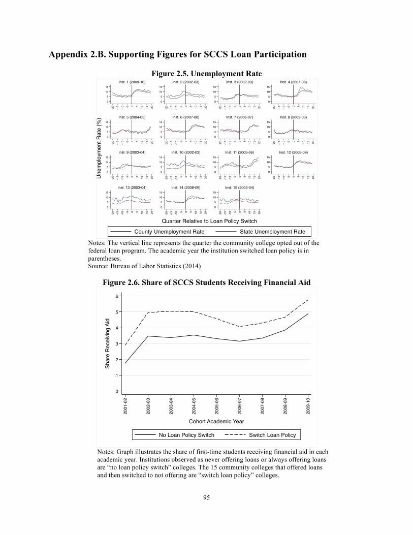
95
Appendix 2.B. Supporting Figures for SCCS Loan Participation
Figure 2.5. Unemployment Rate
Notes: The vertical line represents the quarter the community college opted out of the federal loan program. The academic year the institution switched loan policy is in parentheses. Source: Bureau of Labor Statistics (2014)
Figure 2.6. Share of SCCS Students Receiving Financial Aid
Notes: Graph illustrates the share of first-time students receiving financial aid in each academic year. Institutions observed as never offering loans or always offering loans are “no loan policy switch” colleges. The 15 community colleges that offered loans and then switched to not offering are “switch loan policy” colleges.
0
5
10
15
0
5
10
15
0
5
10
15
0
5
10
15
0
5
10
15
0
5
10
15
0
5
10
15
0
5
10
15
0
5
10
15
0
5
10
15
0
5
10
15
0
5
10
15
0
5
10
15
0
5
10
15
0
5
10
15
-20
-15
-10 -5 0 5 10 15 20 -20
-15
-10 -5 0 5 10 15 20 -20
-15
-10 -5 0 5 10 15 20 -20
-15
-10 -5 0 5 10 15 20
-20
-15
-10 -5 0 5 10 15 20 -20
-15
-10 -5 0 5 10 15 20 -20
-15
-10 -5 0 5 10 15 20 -20
-15
-10 -5 0 5 10 15 20
-20
-15
-10 -5 0 5 10 15 20 -20
-15
-10 -5 0 5 10 15 20 -20
-15
-10 -5 0 5 10 15 20 -20
-15
-10 -5 0 5 10 15 20
-20
-15
-10 -5 0 5 10 15 20 -20
-15
-10 -5 0 5 10 15 20 -20
-15
-10 -5 0 5 10 15 20
Inst. 1 (2009-10) Inst. 2 (2002-03) Inst. 3 (2002-03) Inst. 4 (2007-08)
Inst. 5 (2004-05) Inst. 6 (2007-08) Inst. 7 (2006-07) Inst. 8 (2002-03)
Inst. 9 (2003-04) Inst. 10 (2002-03) Inst. 11 (2005-06) Inst. 12 (2008-09)
Inst. 13 (2003-04) Inst. 14 (2008-09) Inst. 15 (2003-04)
County Unemployment Rate State Unemployment Rate
Une
mpl
oym
ent R
ate
(%)
Quarter Relative to Loan Policy Switch
0
.1
.2
.3
.4
.5
.6
Shar
e R
ecei
ving
Aid
2001
-02
2002
-03
2003
-04
2004
-05
2005
-06
2006
-07
2007
-08
2008
-09
2009
-10
Cohort Academic Year
No Loan Policy Switch Switch Loan Policy
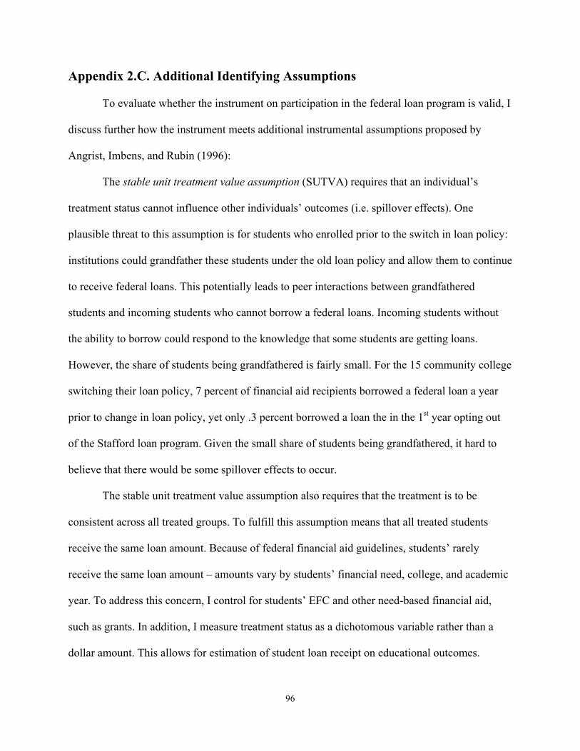
96
Appendix 2.C. Additional Identifying Assumptions To evaluate whether the instrument on participation in the federal loan program is valid, I
discuss further how the instrument meets additional instrumental assumptions proposed by
Angrist, Imbens, and Rubin (1996):
The stable unit treatment value assumption (SUTVA) requires that an individual’s
treatment status cannot influence other individuals’ outcomes (i.e. spillover effects). One
plausible threat to this assumption is for students who enrolled prior to the switch in loan policy:
institutions could grandfather these students under the old loan policy and allow them to continue
to receive federal loans. This potentially leads to peer interactions between grandfathered
students and incoming students who cannot borrow a federal loans. Incoming students without
the ability to borrow could respond to the knowledge that some students are getting loans.
However, the share of students being grandfathered is fairly small. For the 15 community college
switching their loan policy, 7 percent of financial aid recipients borrowed a federal loan a year
prior to change in loan policy, yet only .3 percent borrowed a loan the in the 1st year opting out
of the Stafford loan program. Given the small share of students being grandfathered, it hard to
believe that there would be some spillover effects to occur.
The stable unit treatment value assumption also requires that the treatment is to be
consistent across all treated groups. To fulfill this assumption means that all treated students
receive the same loan amount. Because of federal financial aid guidelines, students’ rarely
receive the same loan amount – amounts vary by students’ financial need, college, and academic
year. To address this concern, I control for students’ EFC and other need-based financial aid,
such as grants. In addition, I measure treatment status as a dichotomous variable rather than a
dollar amount. This allows for estimation of student loan receipt on educational outcomes.
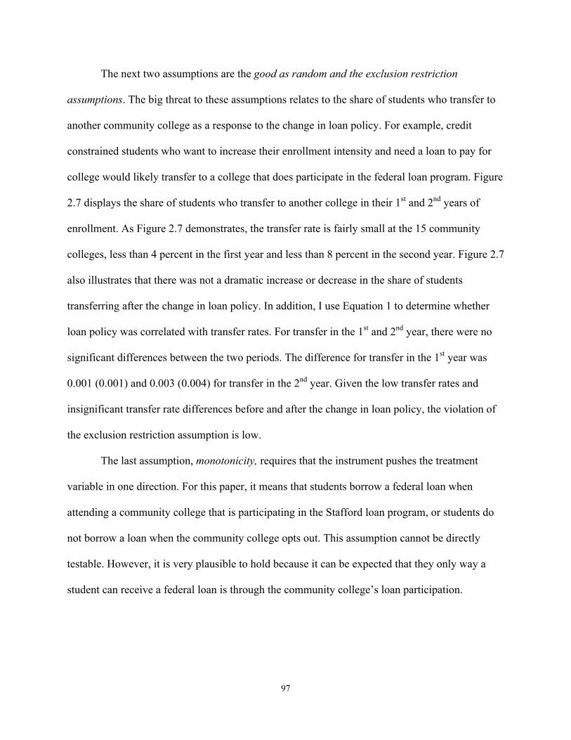
97
The next two assumptions are the good as random and the exclusion restriction
assumptions. The big threat to these assumptions relates to the share of students who transfer to
another community college as a response to the change in loan policy. For example, credit
constrained students who want to increase their enrollment intensity and need a loan to pay for
college would likely transfer to a college that does participate in the federal loan program. Figure
2.7 displays the share of students who transfer to another college in their 1st and 2nd years of
enrollment. As Figure 2.7 demonstrates, the transfer rate is fairly small at the 15 community
colleges, less than 4 percent in the first year and less than 8 percent in the second year. Figure 2.7
also illustrates that there was not a dramatic increase or decrease in the share of students
transferring after the change in loan policy. In addition, I use Equation 1 to determine whether
loan policy was correlated with transfer rates. For transfer in the 1st and 2nd year, there were no
significant differences between the two periods. The difference for transfer in the 1st year was
0.001 (0.001) and 0.003 (0.004) for transfer in the 2nd year. Given the low transfer rates and
insignificant transfer rate differences before and after the change in loan policy, the violation of
the exclusion restriction assumption is low.
The last assumption, monotonicity, requires that the instrument pushes the treatment
variable in one direction. For this paper, it means that students borrow a federal loan when
attending a community college that is participating in the Stafford loan program, or students do
not borrow a loan when the community college opts out. This assumption cannot be directly
testable. However, it is very plausible to hold because it can be expected that they only way a
student can receive a federal loan is through the community college’s loan participation.
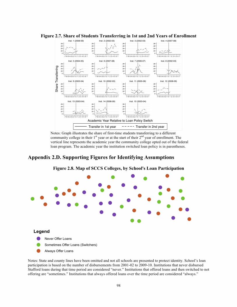
98
Figure 2.7. Share of Students Transferring in 1st and 2nd Years of Enrollment
Notes: Graph illustrates the share of first-time students transferring to a different community college in their 1st year or at the start of their 2nd year of enrollment. The vertical line represents the academic year the community college opted out of the federal loan program. The academic year the institution switched loan policy is in parentheses.
Appendix 2.D. Supporting Figures for Identifying Assumptions
Figure 2.8. Map of SCCS Colleges, by School's Loan Participation
Notes: State and county lines have been omitted and not all schools are presented to protect identity. School’s loan participation is based on the number of disbursements from 2001-02 to 2009-10. Institutions that never disbursed Stafford loans during that time period are considered “never.” Institutions that offered loans and then switched to not offering are “sometimes.” Institutions that always offered loans over the time period are considered “always.”
0.02.04.06.08
0.02.04.06.08
0.02.04.06.08
0.02.04.06.08
0.02.04.06.08
0.02.04.06.08
0.02.04.06.08
0.02.04.06.08
0.02.04.06.08
0.02.04.06.08
0.02.04.06.08
0.02.04.06.08
0.02.04.06.08
0.02.04.06.08
0.02.04.06.08
-7 -6 -5 -4 -3 -2 -1 0 1 2 3 4 5 6 7 -7 -6 -5 -4 -3 -2 -1 0 1 2 3 4 5 6 7 -7 -6 -5 -4 -3 -2 -1 0 1 2 3 4 5 6 7 -7 -6 -5 -4 -3 -2 -1 0 1 2 3 4 5 6 7
-7 -6 -5 -4 -3 -2 -1 0 1 2 3 4 5 6 7 -7 -6 -5 -4 -3 -2 -1 0 1 2 3 4 5 6 7 -7 -6 -5 -4 -3 -2 -1 0 1 2 3 4 5 6 7 -7 -6 -5 -4 -3 -2 -1 0 1 2 3 4 5 6 7
-7 -6 -5 -4 -3 -2 -1 0 1 2 3 4 5 6 7 -7 -6 -5 -4 -3 -2 -1 0 1 2 3 4 5 6 7 -7 -6 -5 -4 -3 -2 -1 0 1 2 3 4 5 6 7 -7 -6 -5 -4 -3 -2 -1 0 1 2 3 4 5 6 7
-7 -6 -5 -4 -3 -2 -1 0 1 2 3 4 5 6 7 -7 -6 -5 -4 -3 -2 -1 0 1 2 3 4 5 6 7 -7 -6 -5 -4 -3 -2 -1 0 1 2 3 4 5 6 7
Inst. 1 (2008-09) Inst. 2 (2002-03) Inst. 3 (2002-03) Inst. 4 (2007-08)
Inst. 5 (2004-05) Inst. 6 (2007-08) Inst. 7 (2006-07) Inst. 8 (2002-03)
Inst. 9 (2003-04) Inst. 10 (2002-03) Inst. 11 (2005-06) Inst. 12 (2008-09)
Inst. 13 (2003-04) Inst. 14 (2008-09) Inst. 15 (2003-04)
Transfer in 1st year Transfer in 2nd year
Shar
e Tr
ansf
errin
g
Academic Year Relative to Loan Policy Switch
!
!
!!
!
!
!
!
!
!!
!
!
! !
!!
! !
!
!
! !
!
!
!
!
!
! !!!!!
!
!
!
!
!
!!
!!
!
!
!
!
!
!
!
!
!
!
!
Legend! Never Offer Loans
! Sometimes Offer Loans (Switchers)
! Always Offer Loans

99
Figure 2.9. Share of Students Attending College in Neighboring County or Far Distance
Notes: Location of student’s high school determines location to community college and is only available for students who reported a high school to the community college. The vertical line represents the academic year the community college opted out of the federal loan program. The academic year the institution switched loan policy is in parentheses.
Figure 2.10. First-Time, First Year Enrollment Rates
Notes: Graph illustrates the share of first-time, first year students enrolling for each academic year. The vertical line represents the academic year the community college opted out of the federal loan program. The academic year the institution switched loan policy is in parentheses.
0
.2
.4
.6
0
.2
.4
.6
0
.2
.4
.6
0
.2
.4
.6
0
.2
.4
.6
0
.2
.4
.6
0
.2
.4
.6
0
.2
.4
.6
0
.2
.4
.6
0
.2
.4
.6
0
.2
.4
.6
0
.2
.4
.6
0
.2
.4
.6
0
.2
.4
.6
0
.2
.4
.6
-8 -6 -4 -2 0 2 4 6 8 -8 -6 -4 -2 0 2 4 6 8 -8 -6 -4 -2 0 2 4 6 8 -8 -6 -4 -2 0 2 4 6 8
-8 -6 -4 -2 0 2 4 6 8 -8 -6 -4 -2 0 2 4 6 8 -8 -6 -4 -2 0 2 4 6 8 -8 -6 -4 -2 0 2 4 6 8
-8 -6 -4 -2 0 2 4 6 8 -8 -6 -4 -2 0 2 4 6 8 -8 -6 -4 -2 0 2 4 6 8 -8 -6 -4 -2 0 2 4 6 8
-8 -6 -4 -2 0 2 4 6 8 -8 -6 -4 -2 0 2 4 6 8 -8 -6 -4 -2 0 2 4 6 8
Inst. 1 (2008-09) Inst. 2 (2002-03) Inst. 3 (2002-03) Inst. 4 (2007-08)
Inst. 5 (2004-05) Inst. 6 (2007-08) Inst. 7 (2006-07) Inst. 8 (2002-03)
Inst. 9 (2003-04) Inst. 10 (2002-03) Inst. 11 (2005-06) Inst. 12 (2008-09)
Inst. 13 (2003-04) Inst. 14 (2008-09) Inst. 15 (2003-04)
Neighboring County Far Distance
Shar
e At
tend
ing
Far F
rom
Hom
e C
ount
y
Academic Year Relative to Loan Policy Switch
.1
.2
.3
.4
.1
.2
.3
.4
.1
.2
.3
.4
.1
.2
.3
.4
.1
.2
.3
.4
.1
.2
.3
.4
.1
.2
.3
.4
.1
.2
.3
.4
.1
.2
.3
.4
.1
.2
.3
.4
.1
.2
.3
.4
.1
.2
.3
.4
.1
.2
.3
.4
.1
.2
.3
.4
.1
.2
.3
.4
-6 -4 -2 0 2 4 6 -6 -4 -2 0 2 4 6 -6 -4 -2 0 2 4 6 -6 -4 -2 0 2 4 6
-6 -4 -2 0 2 4 6 -6 -4 -2 0 2 4 6 -6 -4 -2 0 2 4 6 -6 -4 -2 0 2 4 6
-6 -4 -2 0 2 4 6 -6 -4 -2 0 2 4 6 -6 -4 -2 0 2 4 6 -6 -4 -2 0 2 4 6
-6 -4 -2 0 2 4 6 -6 -4 -2 0 2 4 6 -6 -4 -2 0 2 4 6
Inst. 1 (2008-09) Inst. 2 (2002-03) Inst. 3 (2002-03) Inst. 4 (2007-08)
Inst. 5 (2004-05) Inst. 6 (2007-08) Inst. 7 (2006-07) Inst. 8 (2002-03)
Inst. 9 (2003-04) Inst. 10 (2002-03) Inst. 11 (2005-06) Inst. 12 (2008-09)
Inst. 13 (2003-04) Inst. 14 (2008-09) Inst. 15 (2003-04)
Shar
e Fi
rst-T
ime
Enro
llees
Academic Year Relative to Loan Policy Switch
100
Chapter 3. Student Aid Simplification: Looking Back and Looking Ahead*
3.1. Introduction
Each year, 14 million households seeking federal aid for college complete a detailed
questionnaire about their finances, the Free Application for Federal Student Aid (FAFSA). With
116 questions, the FAFSA is almost as long as IRS Form 1040 and substantially longer than
Forms 1040EZ and 1040A. Since the majority of households use the shorter IRS forms, the
typical household’s aid application is longer and more complicated than its federal tax return.
Aid for college is intended to increase college attendance by reducing its price and loosening
liquidity constraints. Economic theory, empirical evidence and common sense suggest that
complexity in aid could undermine its ability to affect schooling decisions.
A long-standing theoretical and experimental literature suggests that seemingly minor
differences in program design can have profound impacts upon decision-making (Kahneman &
Tversky, 2000). A burgeoning empirical literature has demonstrated that these predictions hold
in real-life situations such as saving for retirement (Madrian & Shea, 2001). Empirical patterns in
the behavioral impact of aid have supported the hypothesis that complexity in the aid system
undermines its efficacy: simple aid programs have a robust impact on college attendance, while
traditional forms of student aid (which require a FAFSA) do not (Dynarski & Scott-Clayton,
2006). A recent field experiment directly tested this hypothesis by randomly assigning families
* Co-authored with Dr. Susan Dynarski and published in the National Tax Journal, vol. 65, p. 211-234.
101
to a radically simplified aid application process (Bettinger, Long, Oreopoulos, & Sanbonmatsu,
2012). The results were striking: a simplified aid application process produced a substantial
increase in college attendance, comparable to that induced by offering an applicant several
thousand dollars in grant aid. Based on these results and a review of other interventions intended
to increase college attendance, Dynarski, Hyman, and Schanzenbach (2011) calculate that
simplifying the aid process is (by several orders of magnitude) the cheapest way to increase
college attendance.
Five years ago, Dynarski and Scott-Clayton (2006) published an analysis of complexity
in the aid system that generated considerable discussion in academic and policy circles. Over the
next few years, complexity in the aid system drew the attention of the media, advocacy groups,
presidential candidates, the National Economic Council, and the Council of Economic Advisers.
A flurry of legislative and agency activity around aid simplification followed. In this article, we
provide a retrospective of what has changed in the aid application process, what has not, and the
possibilities for future reform.
3.2. Background: A Brief Overview of Aid for College
In this section we briefly describe how the financial aid system functions in the United
States and how it evolved into its current shape.33 Two programs represent the bulk of federal aid
to college students: the Pell Grant and the Stafford Loan. Both are distributed through the “need-
determination” process, in which extensive data about a student's resources and expenses are
used to estimate his or her “need” for aid. The FAFSA is required for all federal grants and
loans. Most state aid and school scholarships also require the FAFSA. Some colleges require an
additional aid application. The FAFSA collects basic demographics (e.g., name, social security
33 Some of this material is drawn from Dynarski and Scott-Clayton (2006), where this topic is covered in greater detail.
102
number, citizenship, date of birth) as well as detailed information about the student's and parents'
income, assets, and expenditures.
Once the FAFSA is submitted, the U.S. Department of Education (ED) computes the
Expected Family Contribution (EFC), an estimate of how much the family can pay out of pocket
for college. “Need” is defined as the difference between the cost of attendance (e.g., tuition, fees,
books, and living expenses) and this family contribution. Using the EFC, colleges personalize a
package of grants and loans for each student, which they then mail out in award letters, typically
in March and April. Only upon receiving these award letters do students know how much
college will cost for the upcoming academic school year.
The current aid application has its historical roots in a form developed by a group of
private colleges in the 1950’s. The colleges, under the auspices of the College Board, worked
together to establish a common method for assigning aid so that they could prevent competitive
bidding for students. They established a common aid application (the Parents' Confidential
Statement) and formed the College Scholarship Service (CSS) to process the application (Duffy
& Goldberg, 1998; Wilkinson, 2005). The form was intended to measure income and wealth at
quite high levels, reflecting the student composition of the founding colleges (e.g., Harvard). The
form asked, for example, about the model of the family car. At the time that this first aid form
was designed, there was no federal aid application to work from, since the Pell Grant and student
loan programs had yet to be created. The private institutions were the first architects of aid in the
US, and their imprint is clear in the current system.
In 1973, the most ambitious aid program was established: the federal Pell Grant, first
known as the Basic Education Opportunity Grant (BEOG). The Pell was introduced in a context
of small, scattered state and institutional aid programs, which often had their own applications.

103
Concerned about the multiple forms faced by students seeking aid for college, a group of
financial aid stakeholders came together in 1975 as the National Task Force on Student Aid
Programs, or the Keppel Task Force. The group succeeded in getting cooperation from
institutions, states and the federal government in the development of a common application for
student aid. A common aid application need not have implied a common formula for defining a
student's aid eligibility, any more than the Common Application now used by 456 colleges
defines a single standard for college admission.34 However, as part of the initiative that created
the common form, the various players also agreed upon a common formula, initially known as
the Uniform Methodology and now known as the Federal Methodology.
The model established in 1975 persists today: a common application for collecting
extensive data about a student's finances (the FAFSA) linked to a common formula (the Federal
Methodology) for translating these data into a metric of a student's ability to pay (the Expected
Family Contribution). Federal, state and institutional aid programs use the EFC to determine aid
eligibility.
The contents of the FAFSA and the definition of the EFC are controlled by the federal
government. In its periodic reauthorizations of the 1965 Higher Education Act, Congress makes
decisions about aid, which are then implemented by ED. ED has considerable discretion in its
implementation of Congressional intent. ED's decisions about how to implement a given
directive can add complexity to the aid process. For example, in 2008, Congress directed ED to
allow homeless applicants to complete a shortened application. In response, ED added three
questions to the FAFSA that elicit whether a student has been defined as homeless by a list of
state and local agencies. This is a case in which a Congressional directive to simplify the process
for a minority of applicants led to an increase in complexity for all applicants. 34 A list of colleges using the Common Application can be found at http://www.commonapp.org.

104
3.3. Complexity in the Aid System: Critiques and Responses
In 2005, the Advisory Committee on Student Financial Assistance, a Congressionally
authorized standing committee, released a report that critiqued complexity in the financial aid
system (Advisory Committee on Student Financial Assistance, 2005). The committee concluded
that:
“Millions of students and adult learners who aspire to college are overwhelmed by the complexity of student aid. Uncertainty and confusion robs them of its significant benefits. Rather than promote access, student aid often creates a series of barriers - a gauntlet that the poorest students must run to get to college.” (p. i) Dynarski and Scott-Clayton (2006) quantified complexity in the aid system. That article showed
that the FAFSA rivals the IRS tax forms in length, with more questions than the 1040EZ, 1040A
or even the 1040. That article also demonstrated that there is very little tradeoff between
simplicity and targeting in the federal aid programs, since the majority of questions on the
FAFSA have little marginal impact on federal aid eligibility. A small handful of the questions —
in particular, income and family size — account for about 80 percent of the variation in Pell
grant eligibility. Most of the questions could therefore be removed from the FAFSA while
maintaining the existing distribution of aid.
This research was cited in the 2006 report of the Commission on the Future of Higher
Education, which had been charged by then-Secretary of Education Margaret Spellings to
identify challenges facing the higher education system in the United States. The Commission
called for “consolidating programs, streamlining processes, and replacing the FAFSA with a
much shorter and simpler application (Commission on the Future of Higher Education, 2006, p.
3) .” The analysis of Dynarski and Scott-Clayton (2006) was developed into a policy proposal to
streamline the aid application process and released by the Hamilton Project in 2007 (Dynarski &
Scott-Clayton, 2007). Elements of this proposal were integrated into the platforms of several of
105
the presidential candidates, including that of Barack Obama, and ultimately were included in the
Democratic national platform. In 2008, a working group of academics and aid officials released a
report sounding similar themes under the auspices of the College Board (Rethinking Student Aid
Study Group, 2008).
In 2007, Congress responded to the rising chorus of criticism of the aid application by
including several simplifications in the College Cost Reduction and Access Act (CCRAA).
These provisions did not take effect until the 2009–10 academic year. CCRAA eliminated
portions of the FAFSA, including Worksheet A, which had asked about untaxed income. But
CCRAA also imposed new requirements for determining if a student was an independent,
thereby adding questions to the FAFSA. CCRAA also expanded the number of students who
automatically qualified for a family contribution of zero (an “auto-zero EFC”). Before CCRAA,
households with annual income below $20,000 were eligible for the auto-zero EFC; CCRAA
raised that threshold to $30,000 (U.S. Department of Education, 2008c).
Upon Barack Obama's election, ED, the National Economic Council, and the Council of
Economic Advisers began working on efforts to streamline the aid process, releasing in
September 2009 a report devoted to the topic (Council of Economic Advisors, 2009) that drew
extensively upon Dynarski and Scott-Clayton (2006), Dynarski and Scott-Clayton (2007) and the
report of the Rethinking Student Aid Study Group (2008). During the summer of 2009,
Congressional committees developed ambitious legislation to streamline the aid form. Most of
these provisions were eventually discarded in last-minute negotiations, which were dominated by
legislation to overhaul student loans and health care.
Since this burst of Congressional activity, the most significant changes to the aid system
have been made via administrative authority. ED has worked to simplify the online FAFSA,

106
eliminating repetitive questions (e.g., applicants had previously been asked for their age as well
as their birth date) and introducing “skip logic” that allows students and parents to answer fewer
questions based on their responses to screening questions (U.S. Department of Education,
2010b).
In the spring of 2010, some online applicants were for the first time allowed to
automatically transfer their IRS data into the FAFSA application. This process saves applicants
from having to collect tax documents and enter items manually. This in turn prevents data-entry
errors, which cause applications to be flagged for revision and resubmission.35 This represented a
major administrative breakthrough, since IRS had steadfastly refused to allow any such
connection of data from the two agencies, citing both privacy concerns and a longstanding
resistance to using tax data for any purpose other than tax collection. Both of these issues were
resolved to IRS's satisfaction by having applicants personally log into IRS servers while filling in
the FAFSA, with data items then copied over to the aid form via the applicant's web browser.
This effort to streamline the online application was paired with an ongoing campaign to
move applicants away from the paper FAFSA. ED stopped accepting bulk orders for the paper
FAFSA, which had been placed annually by colleges, high schools, college coaching programs,
libraries, and community agencies. This meant, for example, that students were no longer able to
go to their high school guidance counselor to get a copy of the FAFSA, but had to instead order
one from ED. Paper applications dropped sharply, from 696,000 filed by undergraduates in
2006–07 to 500,000 the following year (U.S. Department of Education, 2008a, 2009b). In 2009–
10, only 94,000 paper FAFSA applications were submitted (U.S. Department of Education,
2011a).
35 ED has for a number of years sent FAFSAs to IRS to have them checked for errors in income and tax data. Upon discovering an inconsistency, IRS flags the application, which ED then returns to the applicant for revision. IRS does not specify (to ED or the applicant) which answer is in error.
107
In another important development, completing the FAFSA online (but not on paper) now
produces an immediate estimate of federal aid eligibility, just as completing a 1040 produces an
estimate of tax liability. Previously, applicants received no notification of aid eligibility until
they received an award letter from the aid offices of the colleges to which they had been
admitted.
3.4. What Has Changed? What Has Not Changed?
We have just described quite a bit of legislative and agency activity. What has been the
net effect on the applicant experience? Is applying for aid less of a hurdle than it was in 2006?
3.4.1. FAFSA Still Longer than Typical Federal Tax Return
The FAFSA still makes the typical tax return look svelte. While two dozen questions
have been removed from the FAFSA in the past five years, another dozen have been added. As a
result, the FAFSA now has 116 questions, compared to 127 questions five years ago.36 In Table
3.1, we compare the 2011–12 FAFSA to its 2006–07 incarnation, as well as to the 1040, 1040A
and 1040EZ for the 2010 tax year. The FAFSA is now slightly shorter than the 1040, at 116 and
126 questions, respectively. In 2006, by contrast, the FAFSA was slightly longer. Since more
than half of families with incomes in the Pell range (that is, below $50,000) fill out the 1040A or
1040EZ,37 the shorter tax forms may be a more appropriate benchmark. The FAFSA compares
poorly with these shorter IRS forms: the 1040EZ has 38 questions and the 1040A has 84,
compared to the FAFSA's 116. Nine data items on the 1040EZ (44 on the 1040A) are used to
compute tax liability, as compared to the 66 FAFSA questions used to compute aid eligibility. As
36 Dropped questions include eight pertaining to earned income credits, additional child tax credits, welfare benefits, and untaxed social security benefits, two relating to veteran benefits, four pertaining to untaxed income and income adjustments, six calculation lines, one on planned enrollment intensity and two about the colleges to which the FAFSA is being forwarded. Added questions address tax credits and allowances (four questions), dependency status (six questions), the student's high school name and location, parents' email address, dislocated-worker status, and means-tested benefits. 37 Authors' calculations using published tables in Parisi (2011).

108
was true in 2006, it is a puzzle why the aid system requires so much more data than the tax
system to determine ability to pay.
Table 3.1. Complexity of IRS Tax Forms versus FAFSA 1040 1040A 1040EZ FAFSA FAFSA 2010 2010 2010 2006–2007 2011–2012 Number of pages (excluding instructions) 2 2 1 5 6
Number of questions 126 84 38 127 116
Answered through IRS data link 18 Non-financial items
Identifying information 6 6 6 22 24 Demographic/family information 8 8 2 18 29 Enrollment status/school 0 0 0 7 4 Signature and preparer 12 12 12 8 8 Other 1 1 1 10 7
Financial items
Earned income 1 1 1 5 5 Other income 19 12 2 33 19 Assets 0 0 0 6 6 Deductions/credits/allowances 42 23 3 12 14 Calculations from tables 21 12 6 6 0 Withholdings, refund preferences 16 9 5 0 0
Number of items required for computation of tax or aid 76 44 9 72 66
Number words in signing statement 49 64 59 232 232 Official estimate of hours to prepare
Paper 23 9 7 1 3 Web 1
Notes: Counts for the FAFSA are for dependent students with two parents and include questions on required student and parent worksheets. Total number of questions includes sub-questions and non-numbered questions. Items such as name and address are counted in the same way on IRS and FAFSA forms.
3.4.2. Official Estimate of Time to Complete FAFSA Still Implausibly Low
As can be seen in Table 3.1, ED has increased its estimate of time needed to complete the
paper FAFSA, from one hour to three hours:
109
“The time required to complete the paper or PDF version of the FAFSA is estimated to be three hours; the time required to complete the web version of the FAFSA, on FAFSA on the Web, is estimated to be one hour and fifteen minutes; the time required to complete the pre-filled web version of the FAFSA, on FAFSA on the Web, is estimated to be fifty- five minutes. These estimates include the time necessary to review instructions, search data resources, gather the data needed, and complete and review the information collection, and make copies of output documents for future reference.”38 ED was roundly criticized for the implausibility of its earlier estimates, and these new, higher
estimates still seem low. The Paperwork Reduction Act of 1995, which mandates these time
estimates, allows each agency to choose its own method for calculating the time costs of filling
out federal forms, and we know of no detailed exposition of the process ED uses to generate
these estimates. The online FAFSA consists of 19 screens, 116 questions and many pages of
accompanying instructions. ED calculates that online FAFSA applicants spend 23 minutes
logged in and completing the form (U.S. Department of Education, 2011d). Given their overall
estimate of 75 minutes, this indicates ED has concluded that applicants can read the FAFSA
instructions and gather the requisite financial documentation (including that of spouses or
parents) in 52 minutes.
These figures look particularly implausible when compared to the paperwork estimates of
the IRS. The IRS estimates that it takes seven hours to complete the 1040EZ, which is a third the
length of the FAFSA. The IRS estimates it takes 23 hours to complete the 1040, which is slightly
longer than the FAFSA. Outside researchers who have fielded taxpayer surveys have concluded
that even these IRS estimates are low (Blumenthal & Slemrod, 1992). No independent
researchers have conducted a similar survey or observation of how long it takes to complete the
FAFSA, whether on paper or online. The time is ripe for such a study.
38 2012–13 FAFSA instructions, downloaded on January 2, 2012 from http://studentaid.ed.gov.
110
3.4.3. Most Applicants Can't Use FAFSA-IRS Link
The ability of an applicant to link data from his 1040 to his FAFSA has great potential to
simplify the application process. Much of the financial data needed to compute aid eligibility is
present in the IRS data, as are many of the demographic items that the FAFSA requests. As
discussed in Dynarski and Scott-Clayton (2006) and Dynarski and Scott-Clayton (2007), it is
feasible to eliminate the FAFSA completely, with tax data alone used to calculate eligibility.
As implemented, however, the IRS link falls well short of this potential. Applicants are
allowed to import their IRS data only if they have already filed their tax return for the previous
tax year. IRS also needs to have made these newly filed returns available to online aid applicants,
which takes two to eight additional weeks after the return is filed. Given these constraints, it is
virtually impossible for anyone filing under the traditional academic and tax schedules to use the
FAFSA-IRS link. A family who files a 1040 as soon as W-2s are due in household mailboxes
(start of February) would be eligible to use the FAFSA-IRS link sometime between mid-
February and April, while a family who files on tax day would not be able to do so until May or
June. As can be seen in Figure 3.1, most aid applicants have submitted the FAFSA well before
these dates.
Why do so many aid applicants file early in the year? Because schools and aid programs
tell them to. Colleges ask students to file FAFSAs early in the year, as do state aid programs,
whose deadlines are listed on the FAFSA. By mid-April, the date by which an early tax filer
could plausibly use the FAFSA-IRS link, the filing deadline has passed for fifteen state aid
programs, including those in California (March 2) and Illinois (“as soon as possible after January
1”). Students who want to qualify for state aid need to file even earlier than these posted
deadlines (Steinberg, 2011), since some programs give out funds on a first-come, first-served
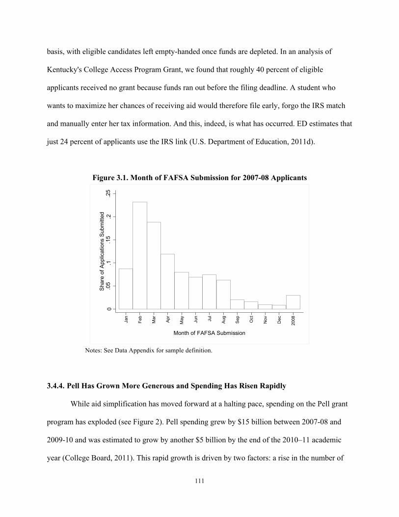
111
basis, with eligible candidates left empty-handed once funds are depleted. In an analysis of
Kentucky's College Access Program Grant, we found that roughly 40 percent of eligible
applicants received no grant because funds ran out before the filing deadline. A student who
wants to maximize her chances of receiving aid would therefore file early, forgo the IRS match
and manually enter her tax information. And this, indeed, is what has occurred. ED estimates that
just 24 percent of applicants use the IRS link (U.S. Department of Education, 2011d).
Figure 3.1. Month of FAFSA Submission for 2007-08 Applicants
Notes: See Data Appendix for sample definition.
3.4.4. Pell Has Grown More Generous and Spending Has Risen Rapidly
While aid simplification has moved forward at a halting pace, spending on the Pell grant
program has exploded (see Figure 2). Pell spending grew by $15 billion between 2007-08 and
2009-10 and was estimated to grow by another $5 billion by the end of the 2010–11 academic
year (College Board, 2011). This rapid growth is driven by two factors: a rise in the number of
0.0
5.1
.15
.2.2
5S
hare
of A
pplic
atio
ns S
ubm
itted
Jan
Feb
Mar
Apr
May Jun
Jul
Aug
Sep Oct
Nov
Dec
2008
Month of FAFSA Submission

112
students attending college and an increase in the generosity of the program. The student
population has grown both due to a demographic blip in the college-age population (Institute of
Education Statistics, 2011) and a persistently weak labor market.
Figure 3.2. Pell Enrollment and Expenditures Relative to 1976-1977 Levels Constant 2010 Dollars
Source: College Board (2011), Figure 13A.
The average Pell has risen sharply; this can occur because the marginal recipient is more needy
or because the program has grown more generous. As we now show, the latter explanation is the
most important one. In Table 3.2, we take full-time, undergraduate aid applicants in the 2007–08
National Postsecondary Student Aid Survey and run their characteristics through the aid
formulas for academic years 2003–04, 2007–08, 2009–10 and 2011–12.39 This analysis
effectively holds constant student characteristics (income, schooling costs, etc.) while allowing
the aid formula to vary. The average Pell for this sample of students rose from $1,417 in 2003– 39 More details about the NPSAS are provided in the Empirical Methodology section and Appendix 3.A.
1
2
3
4
5
6
Am
ount
Rel
ativ
e to
197
6-77
1976
-77
1979
-80
1982
-83
1985
-86
1988
-89
1991
-92
1994
-95
1997
-98
2000
-01
2003
-04
2006
-07
2010
-11
Academic Year
Total Pell Expenditures Number of Pell Recipients
Average Pell Grant per Recipients Max Pell Grant
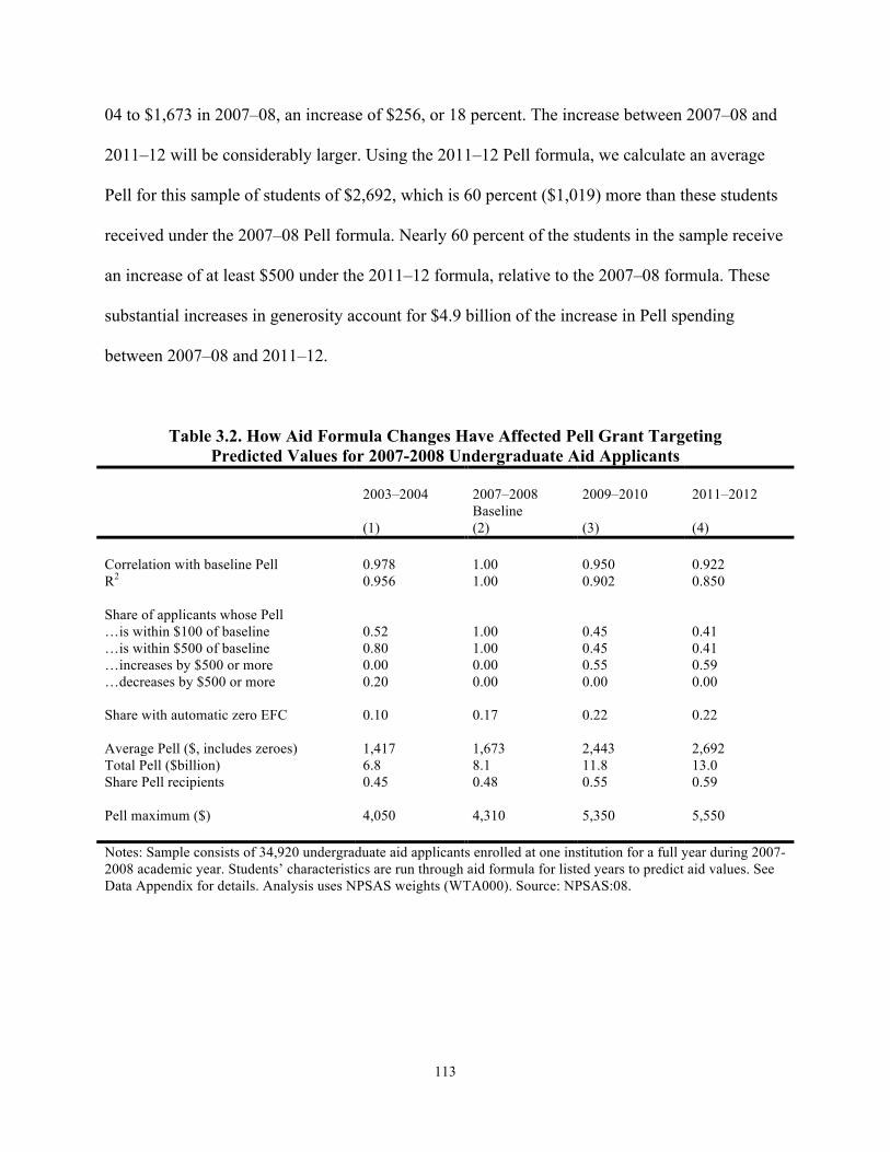
113
04 to $1,673 in 2007–08, an increase of $256, or 18 percent. The increase between 2007–08 and
2011–12 will be considerably larger. Using the 2011–12 Pell formula, we calculate an average
Pell for this sample of students of $2,692, which is 60 percent ($1,019) more than these students
received under the 2007–08 Pell formula. Nearly 60 percent of the students in the sample receive
an increase of at least $500 under the 2011–12 formula, relative to the 2007–08 formula. These
substantial increases in generosity account for $4.9 billion of the increase in Pell spending
between 2007–08 and 2011–12.
Table 3.2. How Aid Formula Changes Have Affected Pell Grant Targeting Predicted Values for 2007-2008 Undergraduate Aid Applicants
2003–2004
2007–2008 Baseline
2009–2010
2011–2012
(1) (2) (3) (4) Correlation with baseline Pell 0.978 1.00 0.950 0.922 R2 0.956 1.00 0.902 0.850 Share of applicants whose Pell …is within $100 of baseline 0.52 1.00 0.45 0.41 …is within $500 of baseline 0.80 1.00 0.45 0.41 …increases by $500 or more 0.00 0.00 0.55 0.59 …decreases by $500 or more 0.20 0.00 0.00 0.00 Share with automatic zero EFC 0.10 0.17 0.22 0.22 Average Pell ($, includes zeroes) 1,417 1,673 2,443 2,692 Total Pell ($billion) 6.8 8.1 11.8 13.0 Share Pell recipients 0.45 0.48 0.55 0.59 Pell maximum ($) 4,050 4,310 5,350 5,550 Notes: Sample consists of 34,920 undergraduate aid applicants enrolled at one institution for a full year during 2007-2008 academic year. Students’ characteristics are run through aid formula for listed years to predict aid values. See Data Appendix for details. Analysis uses NPSAS weights (WTA000). Source: NPSAS:08.
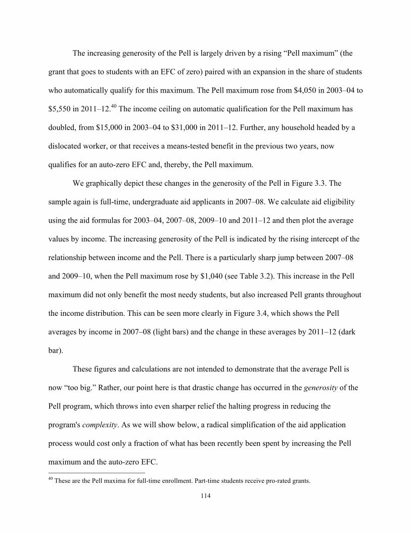
114
The increasing generosity of the Pell is largely driven by a rising “Pell maximum” (the
grant that goes to students with an EFC of zero) paired with an expansion in the share of students
who automatically qualify for this maximum. The Pell maximum rose from $4,050 in 2003–04 to
$5,550 in 2011–12.40 The income ceiling on automatic qualification for the Pell maximum has
doubled, from $15,000 in 2003–04 to $31,000 in 2011–12. Further, any household headed by a
dislocated worker, or that receives a means-tested benefit in the previous two years, now
qualifies for an auto-zero EFC and, thereby, the Pell maximum.
We graphically depict these changes in the generosity of the Pell in Figure 3.3. The
sample again is full-time, undergraduate aid applicants in 2007–08. We calculate aid eligibility
using the aid formulas for 2003–04, 2007–08, 2009–10 and 2011–12 and then plot the average
values by income. The increasing generosity of the Pell is indicated by the rising intercept of the
relationship between income and the Pell. There is a particularly sharp jump between 2007–08
and 2009–10, when the Pell maximum rose by $1,040 (see Table 3.2). This increase in the Pell
maximum did not only benefit the most needy students, but also increased Pell grants throughout
the income distribution. This can be seen more clearly in Figure 3.4, which shows the Pell
averages by income in 2007–08 (light bars) and the change in these averages by 2011–12 (dark
bar).
These figures and calculations are not intended to demonstrate that the average Pell is
now “too big.” Rather, our point here is that drastic change has occurred in the generosity of the
Pell program, which throws into even sharper relief the halting progress in reducing the
program's complexity. As we will show below, a radical simplification of the aid application
process would cost only a fraction of what has been recently been spent by increasing the Pell
maximum and the auto-zero EFC. 40 These are the Pell maxima for full-time enrollment. Part-time students receive pro-rated grants.
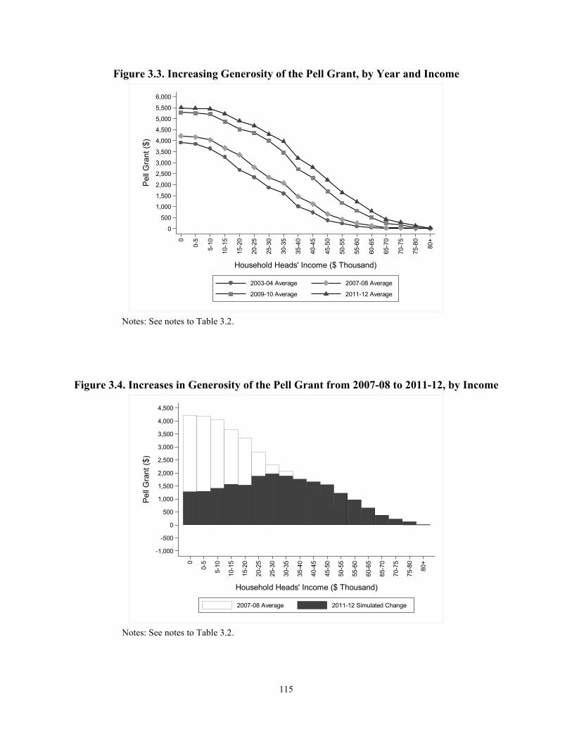
115
Figure 3.3. Increasing Generosity of the Pell Grant, by Year and Income
Notes: See notes to Table 3.2.
Figure 3.4. Increases in Generosity of the Pell Grant from 2007-08 to 2011-12, by Income
Notes: See notes to Table 3.2.
0
500
1,000
1,500
2,000
2,500
3,000
3,500
4,000
4,500
5,000
5,500
6,000
Pel
l Gra
nt ($
)
0
0-5
5-10
10-1
5
15-2
0
20-2
5
25-3
0
30-3
5
35-4
0
40-4
5
45-5
0
50-5
5
55-6
0
60-6
5
65-7
0
70-7
5
75-8
0
80+
Household Heads' Income ($ Thousand)
2003-04 Average 2007-08 Average
2009-10 Average 2011-12 Average
-1,000
-500
0
500
1,000
1,500
2,000
2,500
3,000
3,500
4,000
4,500
Pel
l Gra
nt ($
)
0
0-5
5-10
10-1
5
15-2
0
20-2
5
25-3
0
30-3
5
35-4
0
40-4
5
45-5
0
50-5
5
55-6
0
60-6
5
65-7
0
70-7
5
75-8
0
80+
Household Heads' Income ($ Thousand)
2007-08 Average 2011-12 Simulated Change
116
It is also important to note that the new value of the Pell looks a lot less generous when
viewed in historical context (Figure 3.2). The inflation-adjusted value of the maximum Pell,
which had eroded over time, has now returned to its level when the program was established in
the mid-Seventies. Even with this increase, the maximum Pell has less purchasing power than it
did in the mid-Seventies, since tuition prices have risen much faster than inflation over the past
few decades.
3.5. What Could Be Changed?
We have described the evolution of complexity in the aid system and recent efforts to
reduce it. What are the possibilities for change going forward? Dynarski and Scott-Clayton
(2006) showed, based on 2003–04 data, that the aid system could be massively simplified
without compromising targeting in the Pell. Does this finding still hold? In this section we update
the analysis of Dynarski and Scott-Clayton (2006) using 2007–08 data on student aid and aid
applications. We estimate the marginal contribution of each FAFSA question to variation in Pell
eligibility. We show that the vast majority of questions still have little impact on aid eligibility
and could be eliminated with very little effect on the distribution of aid. We also examine the
effect of using the previous tax year's 1040 data in the calculation of aid. If ED were willing to
use the previous year's tax return to calculate aid eligibility, then all applicants could take
advantage of the IRS-FAFSA link, thereby considerably streamlining the application process.
3.5.1. Empirical Methodology
Using data from the nationally representative 2007–08 National Postsecondary Student
Aid Survey (NPSAS) (U.S. Department of Education, 2009a), we examine the relationship
between federal aid received and information in the FAFSA.41 We focus on Pell Grants, since
41 This description of the methodology used in the analysis is drawn from Dynarski and Scott-Clayton (2006).

117
they are the most expensive component of federal need-based aid. Our sample consists of 35,000
dependent and independent undergraduates who attended college full-time for the full-year in
2007–08 and who applied for federal aid (more details are provided in Appendix 3.A). The
NPSAS sampling weights indicate that these observations represent about 5 million college
students.
We first use the NPSAS to replicate the current distribution of aid. We calculate aid using
the federal financial aid formula and compare these calculated aid amounts with their true values,
which are given in the NPSAS. Our calculations of Pell Grants and EFCs are extremely close to
their true values. Regressing the actual against the predicted values yields an R2 of 0.94 for the
EFC and 0.84 for the Pell.42 These predicted values constitute the baseline against which we
compare aid under various alternative simplification scenarios.
To measure the influence of the various data elements on aid, we sequentially exclude
data items from the aid formula and recalculate aid, and then compare the new estimates to the
baseline values whose calculation is described above. Mechanically, this is achieved by setting
the value of the excluded items to zero (or, sometimes, to their mean). We measure the predictive
power of these simulations with the R2 from regressions of the baseline aid values against their
simulated values under simplification. We also plot average gains and losses against income.
3.5.2. Using Fewer Data Items to Determine Aid Eligibility
We start by throwing out all of the data used in the aid calculation except for items
available on the IRS Form 1040. This opens the door to an application-free Pell, since eligibility
could be calculated using IRS data alone. With this approach, we determine Pell amounts using
the adjusted gross income of the parents and students, taxes paid, state of residence, family size,
42 Unlike Dynarski and Scott-Clayton (2006), we do not exclude observations for which we cannot replicate the Pell or EFC within $1,000, even using all of the data and the exact federal aid formula. As a result, the R2 in these baseline regressions is slightly lower than in their tables.

118
parents’ and independent students’ marital status, type of income tax form filed, and number of
family members in college.
The extensive data we drop in this simulation explain only ten percent of the variation in
aid (Column 2, Table 3.3). With the few variables we include, we explain 89.6 percent of the
variation in the Pell Grant. Our simulated Pell is within $100 of the baseline Pell (which we
estimated using all of the items in the aid formula) for 78 percent of students, and within $500 of
baseline for 88 percent of students. For 73 percent of FAFSA applicants, and half of current Pell
recipients, the Pell does not change by even a dollar.
The changes in the distribution of the Pell resulting from this massive simplification of
the aid form are depicted in Figure 3.5, where we plot average Pell against adjusted gross
income. The light bars depict the average Pell for each income group, using the complete aid
formula. The dark bars represent the change in the average Pell for each income group that
results from using only IRS data to estimate aid eligibility. As is clear from the figure, the
changes are extremely small. The average Pell for this population rises by $73 from a baseline of
$1,673, or 4.4 percent. We estimate that overall Pell spending would rise by about $300 million
for this population. These numbers are dwarfed by the increasing generosity of the Pell: as we
showed earlier, recent changes in Pell generosity have boosted the average Pell by 60 percent,
resulting in an increase in overall Pell spending of nearly $5 billion.
3.5.3. Use Prior Year's 1040 to Determine Aid Eligibility
All applicants, rather than just 24 percent, could benefit from the FAFSA-IRS link if the
requirement were lifted that the applicant had already filed their 1040 for the most recent tax
year. Alternatively, the FAFSA-IRS link could provide data from an earlier year's 1040. For
example, a student applying in early 2012 for aid for 2012–13 could use IRS data from tax year

119
Table 3.3. Effect of Aid Formula Simplification on Distribution of Pell
2007–2008 Full FAFSA
2007-2008 IRS Data Only
(1) (2) Correlation with baseline Pell 1.00 0.947 R2 1.00 0.896 Share of applicants whose Pell …does not change 1.00 0.73 …is within $100 of baseline 1.00 0.78 …is within $500 of baseline 1.00 0.88 …increases by $500 or more 0.07 …decreases by $500 or more 0.04 Average Pell ($, includes zeroes) 1,673 1,746 Total Pell ($billion) 8.1 8.4 Share Pell recipients 0.48 0.49 Items required for calculation of aid 74 8 Notes: See Table 3.2.
Figure 3.5. Effect of Using Only IRS Data to Define Pell Eligibility: 2007-08 Aid Year
Notes: See notes to Table 3.2.
-1,000
-500
0
500
1,000
1,500
2,000
2,500
3,000
3,500
4,000
4,500
Pel
l Gra
nt ($
)
0
0-5
5-10
10-1
5
15-2
0
20-2
5
25-3
0
30-3
5
35-4
0
40-4
5
45-5
0
50-5
5
55-6
0
60-6
5
65-7
0
70-7
5
75-8
0
80+
Household Heads' Income ($ Thousand)
Current Average Simulated Change
120
2010 (rather than 2011) to complete her FAFSA. These data could be used to determine her final
aid eligibility, or as a placeholder until the 1040 is filed for 2011. The latter is effectively what
happens now: most applicants will complete their 2012–13 FAFSA before filing their 2011
taxes, providing estimates of their 2011 tax data in their FAFSA application. They are then
required to update their FAFSA once they file for the 2011 tax year.
As it stands, however, families manually enter these estimates. ED could instead port
from IRS the 2010 tax data, which would serve as an estimate of the 2011 values. Applicants
who are confident that their 2011 tax data will differ substantially from the 2010 values can
choose to manually enter their information. As they do now, families would then receive an
estimate of their aid eligibility based on the 2010 tax return. ED and IRS could automatically
update these values when the 2011 tax form is filed, just as the individual applicant now does.
While these may sound like minor administrative tweaks, these minor tweaks open the
possibility of a nearly automatic aid application. As Kahneman and Tversky (2000) and Thaler
and Sunstein (2008) argue, small differences in administrative requirements can produce
enormous differences in outcomes.
This approach still leaves some uncertainty in final aid eligibility (though no more than
currently exists), since aid may be changed once the 2011 tax form is filed. An alternative that
would allow for both simplicity and certainty in the aid process would be to determine final aid
eligibility based on the previous year's 1040. As we now show, this has little impact on the
targeting of aid while increasing its simplicity and certainty.
In this analysis, we compare aid eligibility based on income from two adjacent tax years.
For this exercise, we need to observe income in two consecutive years for a set of students.
About half of the students in NPSAS who apply for aid for 2007–08 also apply for the following

121
year.43 We estimate 2008–09 aid amounts using the methodology described earlier, first using all
of the elements in the aid formula and then just the subset of items available in the IRS data. We
then replace the IRS data items that were reported on the 2008–09 FAFSA with those reported
on the 2007–08 FAFSA. This simulates the effect of allowing 2008–09 applicants to use data
from the 1040 they filed in 2007 (for the 2006 tax year), rather than from the 1040 they will
eventually file in 2008 (for the 2007 tax year).
Table 3.4 shows the results. In Column 1 we show the baseline aid for this group of
repeat filers for the 2008-2009 school year. Here, aid eligibility is calculated using the full
FAFSA, which includes items gathered from the applicant’s 1040 for the 2007 tax year. In
Column 2, we replace data from the 2007 tax year with data from the 2006 tax year.44 This
simulates the effect of keeping all of the current FAFSA items while allowing all applicants to
use the IRS-FAFSA link. The average Pell rises by $87, or four percent, while overall Pell
expenditures for this population rise by $300 million. For 77 percent of applicants, the Pell
remains within $500 of baseline. For 67 percent of applicants, and 44 percent of Pell recipients,
the Pell does not change at all. These changes are plotted against income (from the 2007 tax
year) in Figure 3.6.
In Column 3 we examine the effect of eliminating all of the FAFSA items except for the
2007 tax data. For this sample of repeat applicants (as was true for the full sample), restricting
the aid formula to IRS data has little effect on aid eligibility, with 72 percent of applicants seeing
43 Ideally, we would undertake this exercise for all students, and not just those who attend for two consecutive years. This would be possible if the 2007-08 NPSAS were matched with tax returns for the 2006 and 2005 tax years. Aid for 2007-08 could then be calculated using the “prior year” tax data from 2006 as well as with the “prior-prior year” tax data from 2005. 44 We inflate these 2006 dollar values to 2007 values using the CPI, which was 2.8 percent between these two years. This prevents a mechanical increase in aid eligibility induced by inflation.
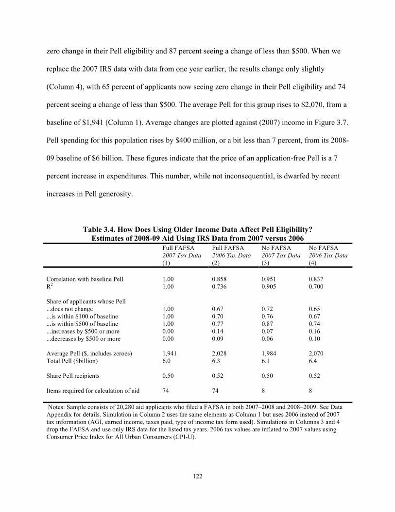
122
zero change in their Pell eligibility and 87 percent seeing a change of less than $500. When we
replace the 2007 IRS data with data from one year earlier, the results change only slightly
(Column 4), with 65 percent of applicants now seeing zero change in their Pell eligibility and 74
percent seeing a change of less than $500. The average Pell for this group rises to $2,070, from a
baseline of $1,941 (Column 1). Average changes are plotted against (2007) income in Figure 3.7.
Pell spending for this population rises by $400 million, or a bit less than 7 percent, from its 2008-
09 baseline of $6 billion. These figures indicate that the price of an application-free Pell is a 7
percent increase in expenditures. This number, while not inconsequential, is dwarfed by recent
increases in Pell generosity.
Table 3.4. How Does Using Older Income Data Affect Pell Eligibility? Estimates of 2008-09 Aid Using IRS Data from 2007 versus 2006
Full FAFSA Full FAFSA No FAFSA No FAFSA 2007 Tax Data 2006 Tax Data 2007 Tax Data 2006 Tax Data (1) (2) (3) (4) Correlation with baseline Pell 1.00 0.858 0.951 0.837 R2 1.00 0.736 0.905 0.700 Share of applicants whose Pell ...does not change 1.00 0.67 0.72 0.65 ...is within $100 of baseline 1.00 0.70 0.76 0.67 ...is within $500 of baseline 1.00 0.77 0.87 0.74 ...increases by $500 or more 0.00 0.14 0.07 0.16 ...decreases by $500 or more 0.00 0.09 0.06 0.10 Average Pell ($, includes zeroes) 1,941 2,028 1,984 2,070 Total Pell ($billion) 6.0 6.3 6.1 6.4 Share Pell recipients 0.50 0.52 0.50 0.52 Items required for calculation of aid 74 74 8 8 Notes: Sample consists of 20,280 aid applicants who filed a FAFSA in both 2007–2008 and 2008–2009. See Data Appendix for details. Simulation in Column 2 uses the same elements as Column 1 but uses 2006 instead of 2007 tax information (AGI, earned income, taxes paid, type of income tax form used). Simulations in Columns 3 and 4 drop the FAFSA and use only IRS data for the listed tax years. 2006 tax values are inflated to 2007 values using Consumer Price Index for All Urban Consumers (CPI-U).
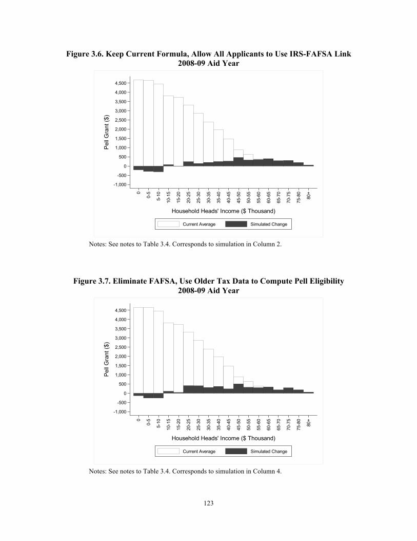
123
Figure 3.6. Keep Current Formula, Allow All Applicants to Use IRS-FAFSA Link 2008-09 Aid Year
Notes: See notes to Table 3.4. Corresponds to simulation in Column 2.
Figure 3.7. Eliminate FAFSA, Use Older Tax Data to Compute Pell Eligibility 2008-09 Aid Year
Notes: See notes to Table 3.4. Corresponds to simulation in Column 4.
-1,000
-500
0
500
1,000
1,500
2,000
2,500
3,000
3,500
4,000
4,500
Pel
l Gra
nt ($
)
0
0-5
5-10
10-1
5
15-2
0
20-2
5
25-3
0
30-3
5
35-4
0
40-4
5
45-5
0
50-5
5
55-6
0
60-6
5
65-7
0
70-7
5
75-8
0
80+
Household Heads' Income ($ Thousand)
Current Average Simulated Change
-1,000
-500
0
500
1,000
1,500
2,000
2,500
3,000
3,500
4,000
4,500
Pel
l Gra
nt ($
)
0
0-5
5-10
10-1
5
15-2
0
20-2
5
25-3
0
30-3
5
35-4
0
40-4
5
45-5
0
50-5
5
55-6
0
60-6
5
65-7
0
70-7
5
75-8
0
80+
Household Heads' Income ($ Thousand)
Current Average Simulated Change
124
3.6. Conclusion
In 2006, Dynarski and Scott-Clayton hypothesized that complexity in the federal aid
program was a barrier to college attendance. That paper also showed that the overwhelming
majority of that complexity did nothing to improve targeting in the Pell Grant. Today, we know
that complexity in the aid program is a barrier to college attendance. The FAFSA field
experiment Bettinger et al. (2012) showed conclusively that a drastically simplified aid
application process increases college attendance. In this experiment, the effect of a simplified
application on college attendance rates was comparable to that of offering an applicant thousands
of dollars in grant aid. Based on these results and a review of other interventions intended to
increase college attendance, Dynarski et al. (2011) calculate that simplifying the aid process is
(by several orders of magnitude) the cheapest way to increase college attendance.
In the face of this evidence, has the aid application process been simplified? There have
been some successes. The user experience for the online FAFSA has been improved, with fewer
repetitive questions and better skip logic. Online applicants are now offered an estimate of their
Pell and Stafford eligibility, a major improvement over the past, when only the EFC was
provided. In a major break through a longstanding administrative logjam, some applicants can
now transfer their IRS tax data directly into their FAFSA from the IRS servers. All of these steps
required sustained administrative energy and attention.
On the downside, the basic structure of the aid application process is unchanged.
Applicants are still faced with a blizzard of paperwork. The FAFSA is just about as long and
complicated as it was in 2006. For every two questions trimmed from the FAFSA, one more
question has been added. As a result the FAFSA has shrunk only slightly (from 127 to 116
questions), and is still longer than the tax forms completed by most taxpayers. The online
125
FAFSA, even with its improved user interface, involves 19 screens and just as many questions as
the paper FAFSA. The IRS-FAFSA link, which has great potential to simplify the aid process, is
hobbled by so many restrictions on its use that only 24 percent of applicants actually use it.
While there has been desultory progress in simplifying the aid system, the generosity and
size of the Pell program have grown by leaps and bounds. Pell spending grew by $15 billion
between 2007–08 and 2009–10 and was estimated to grow by another $5 billion by the end of
2010–11 (College Board, 2011). Drastic change has occurred in the generosity of the Pell
program, which throws into even sharper relief the halting progress in reducing the program's
complexity. A fraction of the dollars spent increasing the Pell maximum could be used to
drastically simplify the aid process, thereby making the dollars that are already being spent more
effective in increasing college attendance. We spend tens of billions of dollars on federal student
aid, and the bill is rising rapidly. Simplifying student aid is a “last-mile” reform that costs little
but requires sustained political and administrative attention.

126
Appendix 3 Appendix 3.A. Data Description
We use individual-level data from the restricted-use version of the 2007-08 National
Postsecondary Student Aid Survey (NPSAS). NPSAS is representative of students filing for aid
for the 2007–08 school year. A subset of students also files a FAFSA for 2008–09, and we limit
the sample to this subset where indicated.
The NPSAS:08 includes FAFSA and financial aid data for 75,710 (11,199,083 survey-
weighted) undergraduate federal aid applicants. We limit the sample to 35,810 (4,951,822
survey-weighted) students enrolled in one institution full-time for the full year during the 2007–
08 academic year. From this sample, 890 (138,858 survey-weighted) students were dropped
because they are missing EFC or data elements needed to calculate EFC. This leaves a sample of
34,920 (4,812,964 survey-weighted) undergraduate federal aid applicants for 2007–08. About
half of these students filed a FAFSA for both the 2007–08 and 2008–09 academic years. For
analyses in which we examine the reliability of older data for estimating aid, this yields a sample
of 20,280 (3,079,184 survey-weighted) students.
In Figures 3.3-3.7, we plot aid values against income. For these graphs, the sample is
divided into twenty intervals. Each interval contains 3 to 6 percent of the sample, except for the
top interval (over $80,000), which contains a quarter of the sample.
127
References Advisory Committee on Student Financial Assistance. (2005). The student aid gauntlet: Making
access to college simple and certain. Washington, DC: Advisory Committee on Student Financial Assistance.
Ang, X., & Jimenez, D. (2014). Private student loans and bankruptcy: Did four-year undergraduates benefit from the increased collectability of student loans? In B. Hershbein & K. M. Hollenbeck (Eds.), Student loans and the dynamics of debt (pp. 235-286). Kalamazoo, MI: W.E. Upjohn Institute for Employment Research.
Angrist, J. D., Imbens, G. W., & Rubin, D. R. (1996). Identification of causal effects using instrumental variables. Journal of the American Statistical Association, 91(434), 444-455.
Association of Private Colleges and Universities v. Arne Duncan, No. 11-1314 (United States District Court for the District of Columbia 2012).
Baum, S. (2015). The evolution of student debt in the United States. In B. Hershbein & K. M. Hollenbeck (Eds.), Student loans and the dynamics of debt (pp. 11-35). Kalamazoo, MI: Upjohn Institute for Employment Research.
Becker, G. S. (1965). A theory of the allocation of time. Economic Journal, 75, 493-517.
Becker, G. S. (1993). Human capital: A theoretical and empirical analysis with special reference to education (3rd ed.). Chicago, IL: The University of Chicago Press.
Best, J., & Best, E. (2014). The student loan mess: How good intentions created a trillion-dollar problem. Berkeley, CA: University of California Press.
Bettinger, E. P., Long, B. T., Oreopoulos, P., & Sanbonmatsu, L. (2012). The role of simplification and information in college decisions: Results from the H&R Block FAFSA experiment. Quarterly Journal of Economics, 127(3), 1205-1242.
Blumenthal, M., & Slemrod, J. (1992). The compliance cost of the U.S. individual income tax system: A second look after tax reform. National Tax Journal, 45(2), 185-202.
Boushey, H. (2005). Student debt: Bigger and bigger. Washington, DC: Center for Economic and Policy Research.
Braunstein, A., McGrath, M., & Pescatrice, D. (2000-2001). Measuring the impact of financial factors on college persistence. Journal of College Student Retention, 2(3), 191-203.
128
Bureau of Labor Statistics. (2014). Local area unemployment statistics (LAUS) [Datafile]. Retrieved from: http://www.bls.gov/data/ - unemployment
Callan, P. (2001). Reframing access and opportunity: Problematic state and federal higher education policy in the 1990s. In D. Heller (Ed.), The state and public higher education policy: Affordability, access, and accountability (pp. 83-99). Baltimore, MD: Johns Hopkins University Press.
Cervantes, A., Creusere, M., McMillion, R., McQueen, C., Short, M., Steiner, M., & Webster, J. (2005). Opening the doors to higher education: Perspectives on the higher education act 40 years later. Roundrock, TX: Texas Guaranteed Student Loan Corporation.
Chen, R., & DesJardins, S. (2008). Exploring the effects of financial aid on the gap in student dropout risks by income level. Research in Higher Education, 49, 1-18.
Cofer, J., & Somers, P. (2000). A comparison of the influence of debt load on the persistence of students at public and private colleges. Journal of Student Financial Aid, 30(2), 39-58.
Cohen, A. M., & Brawer, F. B. (2008). The American community college (5th ed.). San Francisco, CA: Jossey-Bass.
College Board. (2011). Trends in student aid: 2011. Washington, DC: College Board.
College Board. (2013). Trends in student aid: 2013. Washington, DC: College Board.
College Board. (2014a). Trends in college pricing: 2014. Washington, DC: College Board.
College Board. (2014b). Trends in student aid: 2014. Washington, DC: College Board.
Commission on the Future of Higher Education. (2006). A test of leadership: Charting the future of U.S. higher education. Washington, DC: U.S. Department of Education.
Congressional Budget Office. (2006). Cost estimate: Deficit reduction act of 2005. Washington, DC: Congressional Budget Office.
Congressional Budget Office. (2010). Costs and policy options for federal student loan programs. Washington, DC: Congressional Budget Office.
Consumer Financial Protection Bureau. (2013). Student loan affordability: Analysis of public input on impact and solutions. Washington, DC: Consumer Financial Protection Bureau.
Consumers Union. (2007). Helping families finance college: Improved student loan disclosures and counseling. Yonkers, NY: Consumers Union.
Council of Economic Advisors. (2009). Simplifying student aid: The case for an easier, faster, and more accurate FAFSA. Washington, DC: Council of Economic Advisers.
Cunnhinghum, A. F., & Kienzl, G. S. (2011). Delinquency: The untold story of student loan borrowing. Washington, DC: Institute for Higher Education Policy.
129
Darolia, R. (2013). Integrity versus access? The effect of federal financial aid availability on postsecondary enrollment. Journal of Public Economics, 106, 101-114.
Delisle, J. (2012). Federal student loan interest rates: History, subsidies, and cost. Washington, DC: New America Foundation.
Delisle, J., & Miller, B. (2015). Myths & misunderstandings: The undeserved legacy of year-round pell grants. Washington, DC: New America
Delta Cost Project. (2014). IPEDS analytics: Delta cost project database 1987-2010 [Datafile]. Retrieved from: http://nces.ed.gov/ipeds/deltacostproject/
DesJardins, S. L., Ahlburg, D. A., & McCall, B. P. (2002a). Simulating the longitudinal effects of changes in financial aid on student departure. The Journal of Human Resources, 37(3), 653-679.
DesJardins, S. L., Ahlburg, D. A., & McCall, B. P. (2002b). A temporal investigation of factors related to timely degree completion. The Journal of Higher Education, 73(5), 555-581.
Dortch, C., Smole, D. P., & Mahan, S. M. (2010). The SAFRA act: Education reconciliation in the 111th congress. Washington, DC: Congressional Research Service.
Dowd, A. C., & Coury, T. (2006). The effect of loans on the persistence and attainment of community college students. Research in Higher Education, 47, 33-62.
Duffy, E., & Goldberg, I. (1998). Crafting a class: College admissions and financial aid, 1955-1994. Princeton, NJ: Princeton University Press.
Dunlop, E. (2012). What do stafford loans actually buy you? The effect of stafford loan access on community college students. University of Virginia.
Dynarski, S. M. (2003). Loans, liquidity, and schooling decisions. Unpublished. Kennedy School of Government, Harvard University, Cambridge, MA.
Dynarski, S. M., Hyman, J., & Schanzenbach, D. W. (2011). Experimental evidence on the effect of childhood investments on postsecondary attainment and degree completion. (NBER Working Paper 17533). Cambridge, MA: National Bureau of Economic Research Retrieved from http://www.nber.org/papers/w17533.
Dynarski, S. M., & Scott-Clayton, J. E. (2006). The cost of complexity in federal student aid: Lessons from optimal tax theory and behavioral economics. National Tax Journal, 59(2), 319-356.
Dynarski, S. M., & Scott-Clayton, J. E. (2007). College grants on a postcard: A proposal for simple and predictable federal student aid. Washington, DC: The Brookings Institution.
Federal Reserve Bank of New York. (2014). Quarterly report on household debt and credit: August 2014. New York, NY: Federal Reserve Bank of New York.
130
Federal Reserve Bank of New York. (2015). Quarterly report on household debt and credit: February 2015. New York, NY: Federal Researve Bank of New York.
Field, K. (2013). Obama's budget would increase pell grants and add incentives on some student-aid money. The Chronicle of Higher Education. Retrieved August 9, 2013, from http://chronicle.com/article/Presidents-Plan-Would/138473/
Fitzgerald, B. K. (2006). Lowering barriers to college access: Opportunities for more effective coordination of state and federal student aid policies. In P. Gandara, G. Orfield & C. Horn (Eds.), Expanding opportunity in higher education: Leveraging promise (pp. 53-73). Albany, NY: State University of New York Press.
Fossey, R. (1998). The dizzying growth of the federal student loan program: When will vertigo set in? In R. Fossey & M. Bateman (Eds.), Condemning students to debt: College loans and public policy (pp. 7-18). New York, NY: Teachers College Press.
Gardner, L. (2013). Student-loan changes, with lower rates for now, are set to be signed into law. The Chronicle of Higher Education. Retrieved August 9, 2013, from http://chronicle.com/article/New-Student-Loan-Rates-Are-Set/141029/
Gurgand, M., Lorenceau, A., & Melonio, T. (2011). Student loans: Liquidity constraint and higher education in South Africa. Working Paper No. 117. Agence Francaise de Developpement.
Hearn, J. C. (1998). The growing loan orientation in federal financial-aid policy: A historical perspective. In R. Fossey & M. Bateman (Eds.), Condemning students to debt: College loans and public policy (pp. 47-75). New York, NY: Teachers College Press.
Hearn, J. C., & Holdsworth, J. M. (2004). Federal student aid: The shift from grants to loans. In E. P. St. John (Ed.), The public funding of higher education: Changing contexts and new rationales (pp. 40-59). Baltimore, MD: Johns Hopkins University Press.
Hegji, A., Smole, D. P., & Heisler, E. J. (2014). Federal student loan forgiveness and loan repayment programs. Washington, DC: Congressional Research Service.
Heller, D. E. (1997). Student price response in higher education: An update to Leslie and Brinkman. Journal of Higher Education, 68, 624-659.
Hershbein, B., & Hollenbeck, K. M. (2014). The distribution of college graduate debt, 1990-2008: A decomposition approach - updated web tables and figures. Working Paper. W.E. Upjohn Institute for Employment Research, Kalamazoo, MI.
Hershbein, B., & Hollenbeck, K. M. (2015). The distribution of college graduate debt, 1990-2008: A decomposition approach. In B. Hershbein & K. M. Hollenbeck (Eds.), Student loans and the dynamics of debt (pp. 53-116). Kalamazoo, MI: W.E. Upjohn Institute for Employment Research.
131
Hillman, N. W. (2014). College on credit: A multi-level analysis of student loan default. The Review of Higher Education, 37(2), 169-195.
Hobijn, B., Gardiner, C., & Wiles, T. (2011). Recent college graduates and the job market FRBSF Economic Letter. San Francisco, CA: Federal Reserve Bank of San Francisco.
Institute of Education Statistics. (2011). Digest of education statistics: 2011. Washington, DC: U.S. Department of Education.
Institute of Education Statistics. (2012). Digest of education statistics: 2012. Washington, DC: U.S. Department of Education.
Kahneman, D., & Tversky, A. (2000). Choice, values, and frames. Cambridge, MA: Cambridge University Press.
Kamenetz, A. (2006). Generation debt: How our future was sold out. New York, NY: Penguin Group.
Kim, J., Kim, J., DesJardins, S., & McCall, B. (in press). Completing algebra II in high school: Does it increase college access and success? The Journal of Higher Education.
King, J. E. (2007). Who borrows private loans? Washington, DC: American Council on Education.
Kirshstein, R. J., Berger, A. R., Benatar, E., & Rhodes, D. (2004). Workforce contingent financial aid: How states link financial aid to employment, Indianapolis, IN.
Kvaal, J., & Shireman, R. (2004). Money for nothing: Skyrocketing waste of tax dollars on student loan companies' scheme. Oakland, CA: The Institute for College Access and Success.
Laffont, J.-J., & Martimort, D. (2002). The theory of incentives: The principal-agent model. Princeton, NJ: Princeton University Press.
Lane, J. E. (2012). Agency theory in higher education organizations. In M. N. Bastedo (Ed.), The organization of higher education (pp. 278-303). Baltimore, MD: John Hopkins University Press.
Lochner, L., & Monge-Naranjo, A. (2015). Student loans and repayment: Theory, evidence and policy. (NBER Working Paper 20849). Cambridge, MA: National Bureau of Economic Research Retrieved from http://www.nber.org/papers/w20849.
Long, B. T. (2004). The impact of federal tax credits for higher education expenses. In C. M. Hoxby (Ed.), College choices: The economics of where to go, when to go, and how to pay for it (pp. 101-165). Chicago, IL: University of Chicago Press.
Long, B. T. (2007). The contributions of economics to the study of college access and success. Teachers College Record, 109, 2367-2443.

132
Macho-Stadler, I., & Perez-Castrillo, J. D. (2001). An introduction to the economics of information: Incentives and contracts (2nd ed.). New York, NY: Oxford University Press.
Madrian, B. C., & Shea, D. F. (2001). The power of suggestion: Inertia in 401(k) participation and savings behavior. Quarterly Journal of Economics, 116(4), 1149-1187.
Madzelan, D. (2014). The politics of student aid. In A. P. Kelly & S. Goldrick-Rab (Eds.), Reinventing financial aid: Charting a new course to college affordability (pp. 33-74). Cambridge, MA: Harvard Education Press.
Maplethorpe, C. (2001). Advantages and disadvantages of state loan forgiveness and loan repayment programs. NASFAA's Student Aid Transcript, 40-43.
McCallion, G. (2005). Student loan forgiveness programs. Washington, DC: Congressional Research Service.
McSwain, C., Price, D., & Cunningham, A. F. (2006). The future of private loans: Who is borrowing, and why? Washington, DC: Institute for Higher Education Poilcy.
Mettler, S. (2014). Degrees of inequality: How the politics of higher education sabotaged the american dream New York, NY: Basic Books.
Milgrom, P., & Roberts, J. (1992). Economics, organization, and management. Englewood Cliffs, NJ: Prentice-Hall, Inc.
Morris, D., & McGann, E. (2007). Outrage: How illegal immigration, the united nations, congressional ripoffs, student loan overcharges, tobacco companies, trade protection, drug companies are ripping us off ... and what to do about it. New York, NY: Haper Collins Publishers.
Mumper, M. (1996). Removing college price barriers: What government has done and why it doesn't work. Albany, NY: SUNY Press.
National Association of State Student Grant and Aid Programs. (2010). 40th annual survey report on state-sponsored student financial aid: 2008-09 academic year. Washington, DC: National Association of State Student Grant and Aid Programs (NASSGAP) Retrieved from http://www.nassgap.org/viewrepository.aspx?categoryID=3.
National Center for Education Statistics. (2015). Powerstats [Datafile]. Retrieved from: http://nces.ed.gov/datalab/
New York State Office of the Attorney General. (2007). Attorney general Andrew Cuomo reveals deceptive practices In the college loan industry. Retrieved February 1, 2015, from http://www.ag.ny.gov/press-release/attorney-general-andrew-cuomo-reveals-deceptive-practices-college-loan-industry-sends
133
Parisi, M. (2011). Individual income tax returns, preliminary data, 2009. Statistics of Income Bulletin, 31(3), 7-21.
Paulsen, M. B., & Toutkoushian, R. K. (2008). Economic models and policy analysis in higher education: A diagrammatic exposition. In J. C. Smart (Ed.), Higher education: Handbook of theory and research (Vol. 23, pp. 1-48). New York, NY: Agathon Press.
Perrow, C. (1986). Complex organizations: A critical essay (3rd ed.). New York, NY: Random House.
Rethinking Student Aid Study Group. (2008). Fulfilling the commitment: Recommendations for reforming federal student aid. Washington, DC: College Board.
Rothstein, J., & Rouse, C. E. (2010). Constrained after college: Student loans and early-career occupation choices. Journal of Public Economics, 95, 149-163.
Rube, K. (2003). Private loans: Who's borrowing and why? Washington, DC: Public Interest Research Group.
Salas Gage, C., & Lorin, J. (2014). Student loans, the next big threat to the U.S. Economy. Bloomberg Businessweek. Retrieved from http://www.businessweek.com/articles/2014-01-16/student-loans-the-next-big-threat-to-the-u-dot-s-dot-economy
Schenet, M. (1993). Recent changes in federal student aid. Washington, DC: Congressional Research Service.
Shierholz, H., Sabadish, N., & Wething, H. (2012). The class of 2012: Labor market for young graduates remains grim. Washington, DC: Economic Polity Institute.
Skinner, R. R. (2007). Institutional eligibility and the higher education act: Legislative history of the 90/10 rule and its current status. Washington, DC: Congresssional Research Service.
Smole, D. P. (2008). The ensuring continued access to student loans act of 2008. Washington, DC: Congressional Research Service.
Smole, D. P. (2011). Department of education final rules for postsecondary education programs that prepare students for gainful employment in a recognized occupation. Washington, DC: Congressional Research Service.
Smole, D. P. (2013). Federal student loans made under the federal family education loan program and the William D. Ford direct loan programs: Terms and conditions for borrowers. Washington, DC: Congressional Research Service.
Smole, D. P., Kuenzi, J. J., & Skinner, R. R. (2008). The higher education opportunity act: Reauthorization of the higher education act. Washington, DC: Congressional Research Service.
134
Solis, A. (2012). Credit access and college enrollment. Unpublished. Department of Agricultural and Resources Economics, University of California Berkeley, Berkeley, CA.
Spero, I. (1986). The use of student financial aid to attract prospective teachers: A survey of state efforts. Washington, DC: College Entrance Examination Board.
St. John, E. P. (2006). Education and the public interest: School reform, public finance, and access to higher education. Dordrecht, Netherlands: Springer.
Staiger, D., & Stock, J. H. (1997). Instrumental variables regression with weak instruments. Econometrica, 65(3), 557-586.
Steinberg, J. (2011). Seeking Your Questions on the FAFSA, the Free Application for Federal Student Aid. NYTimes.com. Retrieved from http://thechoice.blogs.nytimes.com/2012/01/06/mark-kantrowitz
Stock, J. H., & Yogo, M. (2005). Testing for weak instruments in linear IV regressions. In D. W. K. Andrews & J. H. Stock (Eds.), Identification and Inference for Econometric Models: Essays in Honor of Thomas Rothenberg (pp. 80-108). New York, NY: Combridge University Press.
Stoll, A., Smole, D. P., & Mercer, C. (2007). Student loans, student aid, and FY2008 budget reconciliation. Washington, DC: Congressional Research Service.
Tandberg, D. A. (2010). Politics, interest groups and state funding of public higher education. Research in Higher Education, 51(5), 416-450.
Thaler, R. H., & Sunstein, C. R. (2008). Nudge: Improving decisions about health, wealth, and happiness. New Haven, CT: Yale University Press.
The Institute for College Access & Success. (2008). Denied: Community college students lack access to affordable loans. Oakland, CA: The Institute for College Access & Success.
The Institute for College Access & Success. (2011). Still denied: How community colleges shortchange students by not offering federal loans. Oakland, CA: The Institute for College Access & Success.
The Institute for College Access & Success. (2014a). At what cost? How community colleges that do not offer federal loans put students at risk. Oakland, CA: The Institute for College Access & Success.
The Institute for College Access & Success. (2014b). Student debt and the class of 2013. Oakland, CA: The Instute for College Access & Success.
Toutkoushian, R. K., & Shafiq, M. N. (2010). A conceptual analysis of state support for higher education: Appropriations versus need-based financial aid. Research in Higher Education, 51(1), 40-64.
135
U.S. Department of Education. (2008a). 2006-2007 Federal pell grant program end-of-year report. Washington, DC: U.S. Department of Education.
U.S. Department of Education. (2008b). FY 2009 Department of education justifications of appropriation estimates to the congress: Student loans overview. Washington, DC: U.S. Department of Education.
U.S. Department of Education. (2008c). Summary of changes for the application processing system: 2009-2010. Washington, DC: U.S. Department of Education.
U.S. Department of Education. (2009a). 2007-2008 National postsecondary student aid survey [Restricted Use Datafile]. Retrieved from: http://nces.ed.gov/surveys/npsas/
U.S. Department of Education. (2009b). Federal pell grant program end-of-year report. Washington, DC: U.S. Department of Education.
U.S. Department of Education. (2009c). FY 2010 Department of education justifications of appropriation estimates to the congress: Student loans overview. Washington, DC: U.S. Department of Education.
U.S. Department of Education. (2010a). FY 2011 Department of education justifications of appropriation estimates to the congress: Student loans overview. Washington, DC: U.S. Department of Education.
U.S. Department of Education. (2010b). Summary of changes for the application processing system: 2011-2012. Washington, DC: U.S. Department of Education.
U.S. Department of Education. (2011a). 2009-2010 Federal pell grant program end-of-year report. Washington, DC: U.S. Department of Education.
U.S. Department of Education. (2011b). Academic competitiveness and national SMART grant programs: 2006-07 through 2008-09. Washington, DC: U.S. Department of Education.
U.S. Department of Education. (2011c). Ensuring continued access to student loans act (ECASLA): Annual report to congress. Washington, DC: U.S. Department of Education Retrieved from https://studentaid.ed.gov/about/data-center/lender-guaranty/ecasla.
U.S. Department of Education. (2011d). Federal student aid application: Facts and figures. Washington, DC: U.S. Department of Education.
U.S. Department of Education. (2011e). FY 2012 Department of education justifications of appropriation estimates to the congress: Student loans overview. Washington, DC: U.S. Department of Education.
U.S. Department of Education. (2012). FY 2013 Department of education justifications of appropriation estimates to the congress: Student loans overview. Washington, DC: U.S. Department of Education.
136
U.S. Department of Education. (2013). FY 2014 Department of education justifications of appropriation estimates to the congress: Student loans overview. Washington, DC: U.S. Department of Education.
U.S. Department of Education. (2014a). 2014-2015 Federal student aid handbook.
U.S. Department of Education. (2014b). Digest of education statistics: 2013. Washington, DC: U.S. Department of Education.
U.S. Department of Education. (2014c). Federal student loan portfolio [Dataset]. Retrieved from: https://studentaid.ed.gov/about/data-center/student/portfolio
U.S. Department of Education. (2014d). FY 2015 Department of education justifications of appropriation estimates to the congress: Student loans overview. Washington, DC: U.S. Department of Education.
U.S. Department of Education. (2014e). Integrated postsecondary education data system [Datafile]. Retrieved from: http://nces.ed.gov/ipeds/
U.S. Department of Education. (2014f). Official cohort default rates for schools [Datafile]. Retrieved from: http://ifap.ed.gov/DefaultManagement/press/
U.S. Department of Education. (2014g). Title IV program volume reports [Datafile]. Retrieved from: http://studentaid.ed.gov/about/data-center/student/title-iv
U.S. Department of Education. (2015). FY 2016 Department of education justifications of appropriation estimates to the congress: Student loans overview. Washington, DC: U.S. Department of Education.
U.S. Department of Education Office of Inspector General. (2003). Review of lender inducements (ED/OIG I13C0003). Memorandum. U.S. Department of Education. Washington, DC.
U.S. General Accounting Office. (1991). Vulnerabilities in the stafford student loan program. Washington, DC: U.S. General Accounting Office.
U.S. General Accounting Office. (1992). High-risk series: Student financial aid. Washington, DC: U.S. General Accounting Office.
U.S. General Accounting Office. (1995). High-risk series: Student financial aid. Washington, DC: U.S. General Accounting Office Retrieved from http://www.gao.gov/products/HR-95-10.
U.S. Government Accountability Office. (2004). Federal family education loan program: Statutory and regulatory changes could avert billions in unnecessary federal subsidy payments. Washington, DC: U.S. Government Accountabiilty Office.
137
U.S. Government Accountability Office. (2005). Federal family education loan program: More oversight is needed for schools that are lenders. Washington, DC: U.S. Government Accountability Office.
U.S. Government Accountability Office. (2009). Federal student aid: Recent changes to eligibility requirements and additional efforts to promote awareness could increase academic competitiveness and SMART grant participation. Washington, DC: Government Accountability Office.
U.S. Permanent Senate Subcommittee on Investigations. (1991). Abuses in federal student aid programs. Washington, DC: U.S. Government Printing Office Retrieved from http://files.eric.ed.gov/fulltext/ED332631.pdf.
Waldman, S. (1995). The bill: How the adventures of Clinton's national service bill reveal what is corrupt, comic, cynical, and noble about Washington. New York, NY: Penguin Books.
Wegmann, C. A., Cunningham, A. F., & Merisotis, J. P. (2003). Private loans and choice in financing higher education. Washington, DC: The Institute for Higher Education Policy.
Wiederspan, M. (2011). Understanding service-backed financial aid programs. Unpublished. University of Michigan. Ann Arbor, MI.
Wilkinson, R. (2005). Aiding students, buying students. Nashville, TN: Vanderbilt University Press.